metalog distribution

The metalog distribution is a flexible continuous probability distribution designed for ease of use in practice. Together with its transforms, the metalog family of continuous distributions is unique because it embodies ''all'' of following properties: virtually unlimited shape flexibility; a choice among unbounded, semi-bounded, and bounded distributions; ease of fitting to data with linear least squares; simple, closed-form quantile function (inverse CDF) equations that facilitate simulation; a simple, closed-form PDF; and Bayesian updating in closed form in light of new data. Moreover, like a Taylor series, metalog distributions may have any number of terms, depending on the degree of shape flexibility desired and other application needs.

Applications where metalog distributions can be useful typically involve fitting empirical data, simulated data, or expert-elicited quantiles to smooth, continuous probability distributions. Fields of application are wide-ranging, and include economics, science, engineering, and numerous other fields. The metalog distributions, also known as the Keelin distributions, were first published in 2016 by Tom Keelin.

History

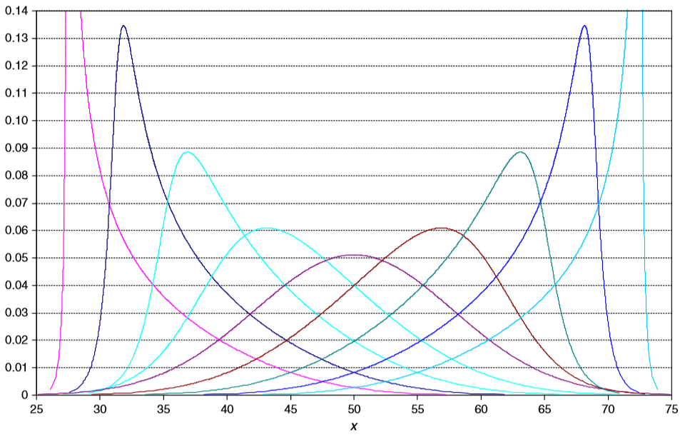
The history of probability distributions can be viewed, in part, as a progression of developments towards greater flexibility in shape and bounds when fitting to data. The normal distribution was first published in 1756, and Bayes’ theorem in 1763. The normal distribution laid the foundation for much of the development of classical statistics. In contrast, Bayes' theorem laid the foundation for the state-of-information, belief-based probability representations. Because belief-based probabilities can take on any shape and may have natural bounds, probability distributions flexible enough to accommodate both were needed. Moreover, many empirical and experimental data sets exhibited shapes that could not be well matched by the normal or other continuous distributions. So began the search for continuous probability distributions with flexible shapes and bounds.

Early in the 20th century, the Pearson family of distributions, which includes the normal, beta, uniform, gamma, student-t, chi-square, F, and five others, emerged as a major advance in shape flexibility. These were followed by the Johnson distributions. Both families can represent the first four moments of data (mean, variance, skewness, and kurtosis) with smooth continuous curves. However, they have no ability to match fifth or higher-order moments. Moreover, for a given skewness and kurtosis, there is no choice of bounds. For example, matching the first four moments of a data set may yield a distribution with a negative lower bound, even though it might be known that the quantity in question cannot be negative. Finally, their equations include intractable integrals and complex statistical functions, so that fitting to data typically requires iterative methods.

Early in the 21st century, decision analysts began working to develop continuous probability distributions that would exactly fit any specified three points on the cumulative distribution function for an uncertain quantity (e.g., expert-elicited $0.10, 0.50$, and $0.90$ quantiles). The Pearson and the Johnson family distributions were generally inadequate for this purpose. In addition, decision analysts also sought probability distributions that would be easy to parameterize with data (e.g., by using linear least squares, or equivalently, multiple linear regression). Introduced in 2011, the class of quantile-parameterized distributions (QPDs) accomplished both goals. While being a significant advance for this reason, the QPD originally used to illustrate this class of distributions, the Simple Q-Normal distribution, had less shape flexibility than the Pearson and Johnson families, and lacked the ability to represent semi-bounded and bounded distributions. Shortly thereafter, Keelin developed the family of metalog distributions, another instance of the QPD class, which is more shape-flexible than the Pearson and Johnson families, offers a choice of boundedness, has closed-form equations that can be fit to data with linear least squares, and has closed-form quantile functions, which facilitate Monte Carlo simulation.

Definition and quantile function

The metalog distribution is a generalization of the logistic distribution, where the term "metalog" is short for "metalogistic". Starting with the logistic quantile function, $x=Q(y)=\mu+s\mbox \ln\Bigl(\Bigr)$, Keelin substituted power series expansions in cumulative probability $y=F(x)$ for the $\mu$ and the $s$ parameters, which control location and scale, respectively.Keelin TW (2016). "The Metalog Distributions." Decision Analysis. 13 (4): 243–277.
/ref>

:$\mu =a_1 + a_4(y -0.5) + a_5(y -0.5)^2 + a_7(y -0.5)^3 + a_9(y -0.5)^4 + \dots$
:$s =a_2 + a_3(y -0.5) + a_6(y -0.5)^2 + a_8(y -0.5)^3 + a_(y -0.5)^4 + \dots$

Keelin's rationale for this substitution was fivefold. First, the resulting quantile function would have significant shape flexibility, governed by the coefficients $a_i$. Second, it would have a simple closed form that is linear in these coefficients, implying that they could easily be determined from CDF data by linear least squares. Third, the resulting quantile function would be smooth, differentiable, and analytic, ensuring that a smooth, closed-form PDF would be available. Fourth, simulation would be facilitated by the resulting closed-form inverse CDF. Fifth, like a Taylor series, any number of terms $k$ could be used, depending on the degree of shape flexibility desired and other application needs.

Note that the subscripts of the $a$-coefficients are such that $a_1$ and $a_4$ are in the $\mu$ expansion, $a_2$ and $a_3$ are in the $s$ expansion, and subscripts alternate thereafter. This ordering was chosen so that the first two terms in the resulting metalog quantile function correspond to the logistic distribution exactly; adding a third term with $a_3 \neq 0$ adjusts skewness; adding a fourth term with $a_4 \neq 0$ adjusts kurtosis primarily; and adding subsequent non-zero terms yields more nuanced shape refinements.

Rewriting the logistic quantile function to incorporate the above substitutions for $\mu$ and $s$ yields the metalog quantile function, for cumulative probability 0.
:$M_k(y)= \left\{ \begin{array}{ll} a_1+a_2\ln\Bigl({y\over{1-y\Bigr) & \mbox{for } k=2\\ a_1+a_2\ln\Bigl({y\over{1-y\Bigr)+a_3(y-0.5) \ln \Bigl({y\over{1-y\Bigr) & \mbox{for } k=3\\ a_1+a_2\ln\Bigl({y\over{1-y\Bigr)+a_3(y-0.5) \ln \Bigl({y\over{1-y\Bigr)+a_4(y-0.5) & \mbox{for } k=4\\ M_{k-1}(y)+a_k(y-0.5)^{k-1\over2} & \mbox{for odd } k\geq5\\ M_{k-1}(y)+a_k(y-0.5)^\Bigr) & \mbox{for even } k\geq6\\ \end{array}\right.$

Equivalently, the metalog quantile function can be expressed in terms of basis functions: $M_k(y) = \sum_{i=1}^k a_i g_i(y)$, where the metalog basis functions are $g_1(y)=1,\mbox{ } g_2(y)=\ln\Bigl({y\over{1 -y\Bigr),$ and each subsequent $g_i(y)$ is defined as the expression that is multiplied by $a_i$ in the equation for $M_k(y)$ above. Note that coefficient $a_1$ is the median, since all other terms equal zero when $y=0.5$. Special cases of the metalog quantile function are the logistic distribution ($k=2$) and the uniform distribution ($k\geq4,a_1 = 0.5,a_4 =1,a_i =0$ otherwise).

Probability density function

Differentiating $x=M_k(y)$ with respect to $y$ yields the quantile density function $q(y)=dx/dy$. The reciprocal of this quantity, $(q(y))^{-1}=dy/dx=f(Q(y))$, is the probability density function expressed as a p-PDF,p-PDF: A probability density function expressed as a function of cumulative probability $y$ rather than variable of interest $x$; equivalently, a "density quantile function" as defined by Parzen, E., 1979, Nonparametric statistical data modeling, Journal of the American Statistical Association,7, 105–131

:$m_k(y)= \left\{ \begin{array}{ll} {y(1-y)\over{a_2 & \mbox{for } k=2\\ \Bigl({a_2\over{y(1-y)+a_3\Bigl({y-0.5\over{y(1-y)+\ln{y\over{1-y\Bigr)\Bigr)^{-1} & \mbox{for } k=3\\ \Bigl({a_2\over{y(1-y)+a_3\Bigl({y-0.5\over{y(1-y)+\ln{y\over{1-y\Bigr)+a_4\Bigr)^{-1} & \mbox{for } k=4\\ \Bigl({1\over{m_{k-1}(y)+a_k{k-1\over2}(y-0.5)^{(k-3)/2}\Bigr)^{-1} & \mbox{for odd } k\geq5\\ \Bigl({1\over{m_{k-1}(y)+a_k\Bigl({(y-0.5)^{k/2-1}\over{y(1-y)+({k\over2}-1)(y-0.5)^{(k/2-2)}\ln{y\over{1-y\Bigr)\Bigr)^{-1} & \mbox{for even } k\geq6,\\ \end{array}\right.$
which may be equivalently expressed in terms of basis functions as

: $m_k(y) = \left( \sum_{i=1}^k a_i \right)^{-1}$ where 0.
Note that this PDF is expressed as a function of cumulative probability, $y$, rather than variable of interest, $x$. To plot the PDF (e.g., as shown in the figures on this page), one can vary $y\in(0,1)$ parametrically, and then plot $x=M_k(y)$ on the horizontal axis and $m_k(y)$ on the vertical axis.

Based on the above equations and the following transformations that enable a choice of bounds, the family of metalog distributions is composed of unbounded, semibounded, and bounded metalogs, along with their symmetric-percentile triplet (SPT) special cases.

Unbounded, semi-bounded, and bounded metalog distributions

As defined above, the metalog distribution is unbounded, except in the unusual special case where $a_i = 0$ for all terms that contain $\ln\Bigl({y\over{1-y\Bigr)$. However, many applications require flexible probability distributions that have a lower bound $b_l$, an upper bound $b_u$, or both. To meet this need, Keelin used transformations to derive semi-bounded and bounded metalog distributions. Such transformations are governed by a general property of quantile functions: for any quantile function $x=Q(y)$ and increasing function $z(x), x=z^{-1} (Q(y))$ is also a quantile function. For example, the quantile function of the normal distribution is $x=\mu+\sigma \Phi^{-1} (y)$; since the natural logarithm, $z(x)=\ln(x-b_l)$, is an increasing function, $x=b_l+e^{\mu+\sigma \Phi^{-1} (y)}$ is the quantile function of the lognormal distribution. Analogously, applying this property to the metalog quantile function $M_k(y)$ using the transformations below yields the semi-bounded and bounded members of the metalog family. By considering $z(x)$ to be metalog-distributed, all members of the metalog family meet Keelin and Powley's definition of a quantile-parameterized distribution and thus possess the properties thereof.
:
\begin{array}{l, c, c, c, c, c}
& & & & & \mbox{shape}\\
& \mbox{transformation} & \mbox{quantile function} & \mbox{PDF} & \mbox{where} &\mbox{parameters}\\
\hline
\mbox{Metalog (unbounded)} & z(x)=x & M_k(y) & m_k(y) & 0
Note that the number of shape parameters in the metalog family increases linearly with the number of terms $k$. Therefore, any of the above metalogs may have any number of shape parameters. By contrast, the Pearson and Johnson families of distributions are limited to two shape parameters.

SPT metalog distributions

The symmetric-percentile triplet (SPT) metalog distributions are a three-term $(k=3)$ special case of the unbounded, semi-bounded, and bounded metalog distributions. These are parameterized by the three $(x,y)$ points off the CDF curve, of the form $(x_1,\alpha)$, $(x_2,0.5)$, and $(x_3,1-\alpha)$, where $0 <\alpha<0.5$. SPT metalogs are useful when, for example, quantiles $(x_1,x_2,x_3)$ corresponding to the CDF probabilities (e.g. $0.1, 0.5, 0.9$) are elicited from an expert and used to parameterize the three-term metalog distributions. As noted below, certain mathematical properties are simplified by the SPT parameterization.

Properties

The metalog family of probability distributions has the following properties.

Feasibility

A function of the form of $M_k(y)$ or any of its above transforms is a feasible probability distribution if and only if its PDF is greater than zero for all $y \in (0,1).$ This implies a feasibility constraint on the set of coefficients $\boldsymbol a=(a_1,...,a_k) \in \R^k$,

: $m_k(y)>0$ for all $y \in (0,1)$.

In practical applications, feasibility must generally be checked rather than assumed. For $k=2$, $a_2>0$ ensures feasibility. For $k=3$ (including SPT metalogs), the feasibility condition is $a_2>0$ and ${, a_3, /a_2}<1.66711$. For $k=4$, a similar closed form has been derived. For $k\geq5$, feasibility is typically checked graphically or numerically.

The unbounded metalog and its above transforms share the same set of feasible coefficients. Therefore, for a given set of coefficients, confirming that $m_k(y)>0$ for all $y \in (0,1)$ is sufficient regardless of the transform in use.

Convexity

The set of feasible metalog coefficients $S_\boldsymbol a=\{\boldsymbol a\in\R^k , m_k(y) > 0$ for all $y\in (0,1)\}$ is convex. Because convex optimization problems require convex feasible sets, this property can simplify optimization problems involving metalogs. Moreover, this property guarantees that any convex combination of the $\boldsymbol a$ vectors of feasible metalogs is feasible, which is useful, for example, when combining the opinion of multiple expertsKeelin, Thomas W., and Ronald A. Howard. (2021). “The Metalog Distributions: Virtually Unlimited Shape Flexibility, Combining Expert Opinion in Closed Form, and Bayesian Updating in Closed Form.” OSF Preprints. doi:10.31219/osf.io/xdg5e.
/ref> or interpolating among feasible metalogs.Keelin, T.W., Chrisman, L. and Savage, S.L. (2019). “The metalog distributions and extremely accurate sums of lognormals in closed form.” WSC '19: Proceedings of the Winter Simulation Conference. 3074–3085.
/ref> By implication, any probabilistic mixture of metalog distributions is itself a metalog.

Fitting to data

The coefficients $\boldsymbol a$ can be determined from data by linear least squares. Given $n$ data points $(x_i,y_i)$ that are intended to characterize a metalog CDF, and an $n \times k$ matrix $\boldsymbol Y$ whose elements consist of the basis functions $g_j (y_i)$, then as long as $\boldsymbol Y^T \boldsymbol Y$ is invertible, the column vector $\boldsymbol a$ of the coefficients $a_i$ is given by $\boldsymbol a=(\boldsymbol Y^T \boldsymbol Y)^{-1} \boldsymbol Y^T \boldsymbol z$, where $n\geq k$ and column vector $\boldsymbol z=(z(x_1),\ldots,z(x_n))$. If $n=k$, this equation reduces to $\boldsymbol a=\boldsymbol Y^{-1} \boldsymbol z$, where the resulting metalog CDF runs through all data points exactly. For SPT metalogs, it further reduces to expressions in terms of the three $(x_i,y_i)$ points directly.

An alternate fitting method, implemented as a linear program, determines the coefficients by minimizing the sum of absolute distances between the CDF and the data, subject to feasibility constraints.Faber, I.J. (2019). Cyber Risk Management: AI-generated Warnings of Threats (Doctoral dissertation, Stanford University).
/ref>

Shape flexibility

According to the metalog flexibility theorem, any probability distribution with a continuous quantile function can be approximated arbitrarily closely by a metalog. Moreover, in the original paper, Keelin showed that ten-term metalog distributions parameterized by 105 CDF points from 30 traditional source distributions (including the normal, student-t, lognormal, gamma, beta, and extreme-value distributions) approximate each such source distribution within a K-S distance of 0.001 or less. Thus, metalog shape flexibility is virtually unlimited.

The animated figure on the right illustrates this for the standard normal distribution, where metalogs with various numbers of terms are parameterized by the same set of 105 points from the standard normal CDF. The metalog PDF converges to the standard normal PDF as the number of terms increases. With two terms, the metalog approximates the normal with a logistic distribution. With each increment in number of terms, the fit gets closer. With 10 terms, the metalog PDF and standard normal PDF are visually indistinguishable.

Similarly, nine-term semi-bounded metalog PDFs with $b_l=0$ are visually indistinguishable from a range of Weibull distributions. The six cases shown to the right correspond to Weibull shape parameters 0.5, 0.8, 1.0, 1.5, 2, and 4. In each case, the metalog is parameterized by the nine $x$ points from the Weibull CDF that correspond to the cumulative probabilities $y = (0.001, 0.02, 0.10, 0.25, 0.5, 0.75, 0.9, 0.98, 0.999)$.

Such convergence is not unique to the normal and Weibull distributions. Keelin originally showed analogous results for a wide range of distributions and has since provided further illustrations.

Median

The median of any distribution in the metalog family has a simple closed form. Note that $y=0.5$ defines the median, and $M_k(0.5)=a_1$ (since all subsequent terms are zero for $y=0.5$). It follows that the medians of the unbounded metalog, log metalog, negative-log metalog, and logit metalog distributions are $a_1$, $b_l+e^{a_1}$, $b_u-e^{-a_1}$, and ${b_l+b_u e^{a_1}\over{1+e^{a_1}$, respectively.

Moments

The $m^{th}$ moment of the unbounded metalog distribution, E ^m=\int_{y=0}^1 {M_k(y)}^m \, dy, is a special case of the more general formula for QPDs. For the unbounded metalog, such integrals evaluate to closed-form moments that are $m^{th}$ order polynomials in the coefficients $a_i$. The first four central moments of the four-term unbounded metalog are:
:
\begin{align}
\text{mean} = {} & a_1 +{a_3\over2}\\ pt\text{variance} = {} &
\pi^2{{a_2}^2\over3}+{{a_3}^2\over{12+\pi^2{{a_3}^2\over{36+a_2a_4
+{{a_4}^2\over{12\\ pt\text{skewness} = {} & \pi^2 {a_2}^2{a_3}+\pi^2 {{a_3}^3 \over{24 + {{{a_2} {a_3} {a_4 \over{2+ \pi^2{{{a_2} {a_3} {a_4 \over{6 + {{{a_3} {a_4}^2} \over{8\\ pt\text{kurtosis} = {} & 7\pi^4 {{a_2}^4\over{15+3\pi^2 {{{a_2}^2{a_3}^2}
\over{24+7\pi^4 {{{a_2}^2{a_3}^2} \over{30+{{{a_3}^4}\over{80 +
\pi^2{{a_3}^4 \over{24 + 7\pi^4 {{a_3}^4\over{1200 + 2\pi^2{a_2}^3{a_4}\\ pt& {} +{{{a_2} {a_3}^2 {a_4 \over{2+2\pi^2{{{a_2}
{a_3}^2 {a_4 \over{3+2{{a_2}^2 {a_4}^2}+\pi^2{{{a_2}^2 {a_4}^2 }
\over{6+{{{a_3}^2 {a_4}^2 } \over{8+\pi^2{{{a_3}^2 {a_4}^2 } \over{40+{{{a_2} {a_4}^3 } \over{3 +{{a_4}^4 \over{80 \end{align}
Moments for fewer terms are subsumed in these equations. For example, moments of the three-term metalog can be obtained by setting $a_4$ to zero. Moments for metalogs with more terms, and higher-order moments ($m>4$), are also available. Moments for semi-bounded and bounded metalogs are not available in closed form.

Parameterization with moments

Three-term unbounded metalogs can be parameterized in closed form with their first three central moments. Let $m, v,$ and $s$ be the mean, variance, and skewness, and let $s_s$ be the standardized skewness, $s_s=s/v^{3/2}$. Equivalent expressions of the moments in terms of coefficients, and coefficients in terms of moments, are as follows:

:
\begin{array}{ll}
m = a_1 +{a_3\over2} && a_1 = m -{a_3\over2}\\ ptv =
\pi^2{{a_2}^2\over3}+{{a_3}^2\over{12+\pi^2{{a_3}^2\over{36 &&
a_2 = {1\over{\pi\Bigl \Bigl(v-\Bigl({1\over{12+{{\pi}^2\over{36\Bigr){a_3}^2\Bigr)\Bigr{1\over{2 \\ pts = \pi^2 {a_2}^2{a_3}+\pi^2 {{a_3}^3 \over{24 &&
a_3 = 4\Bigl({6v\over{6+\pi^2\Bigr)^{1\over{2\cos\Bigl 1\over{3\Bigl(\cos^{-1}\Bigl(-{s_s\over{4\Bigl(1+{{\pi}^2\over{6\Bigr)^{1\over{2\Bigr)+4\pi\Bigr)\Bigr\\ pt \end{array}

The equivalence of these two sets of expressions can be derived by noting that the moments equations on the left determine a cubic polynomial in terms of the coefficients $a_1, a_2,$ and $a_3$, which can be solved in closed form as functions of $m, v,$ and $s$. Moreover, this solution is unique.{{Cite web, title=Equivalence of coefficients' and moments' parameterizations of three-term metalog, url=http://www.metalogdistributions.com/n3momentsparameters.html, access-date=2021-03-28, website=www.metalogdistributions.com In terms of moments, the feasibility condition is $, s_s, \leq 2.07093$, which can be shown to be equivalent to the following feasibility condition in terms of the coefficients: $a_2>0$; and ${, a_3, /a_2}<1.66711$.

This property can be used, for example, to represent the sum of independent, non-identically distributed random variables. Based on cumulants, it is known that for any set of independent random variables, the mean, variance, and skewness of the sum are the sums of the respective means, variances, and skewnesses. Parameterizing a three-term metalog with these central moments yields a continuous distribution that exactly preserves these three moments, and accordingly provides a reasonable approximation to the shape of the distribution of the sum of independent random variables.

Simulation

Since their quantile functions are expressed in closed form, metalogs facilitate Monte Carlo simulation. Substituting uniformly distributed random samples of $y$ into the Metalog quantile function (inverse CDF) produces random samples of $x$ in closed form, thereby eliminating the need to invert a CDF. See below for simulation applications.

Eliciting and Combining Expert Opinion

Due to their shape flexibility, metalog distributions can be an attractive choice for eliciting and representing expert opinion.Dion, P., Galbraith, N., Sirag, E. (2020). “Using expert elicitation to build long-term projection assumptions.” In Developments in Demographic Forecasting, Chapter 3, pp. 43–62. Springer
/ref> Moreover, if the opinions of multiple experts are expressed as $k$-term metalogs, the consensus opinion may be calculated as a $k$-term metalog in closed form, where the $\boldsymbol a$-coefficients of the consensus metalog are simply a weighted average of those of the individual experts. This result follows from Vincentization, where the consensus quantile function is a weighted average of individual quantile functions.

Bayesian Updating in Closed Form

In a classic paper, Howard (1970) shows how the beta-binomial distribution can be used to update, according to Bayes rule in closed form, uncertainty over the long-run frequency $\phi$ of a coin toss coming up "heads" in light of new coin-toss data. In contrast, if the uncertainty of interest to be updated is defined not by a scalar probability over a discrete event (like the result of a coin toss) but by a probability density function over a continuous variable, metalog Bayesian updating may be used. Under certain conditions, metalog quantile parameters and $\boldsymbol a$-coefficients may be updated in closed form in light of new data according to Bayes rule.

Applications

Due to their shape and bounds flexibility, metalogs can be used to represent empirical or other data in virtually any field of human endeavor.
* Astronomy. Metalogs were applied to assess the risks of asteroid impact.
* Cybersecurity. Metalogs were used in cyber security risk assessment.
* Eliciting and combining expert opinion. Statistics Canada elicited expert opinions on future Canadian fertility rates from 18 experts, which included the use of spreadsheet-based real-time PDF feedback based on five-term metalogs. The individual expert opinions were then weighted and combined into an overall metalog-based forecast.
* Empirical data exploration and visualization. In fish biology, a 10-term log metalog distribution (bounded below at 0) was fit to the weights of 3,474 steelhead trout caught and released on the Babine River in British Columbia during 2006–2010. The bimodality of the resulting distribution has been attributed to the presence of both first-time and second-time spawners in the river, the latter of which tend to weigh more.
* Hydrology. A 10-term semi-bounded metalog was used to model the probability distribution of annual river gauge heights.
* Oil field production. Semi-bounded SPT metalogs were used to analyze biases in projections of oil-field production when compared to observed production after the fact.
* Portfolio management. SPT metalogs have been used to model commercial value of new products and product portfolios.
* Simulation input distributions. To support a bidding decision, uncertainty about the future value of each of 259 financial assets was represented as an SPT metalog. A simulation of total portfolio value was shown to yield more realistic results than a corresponding simulation based on discrete low, median, and high values for each asset.{{cite journal , url=https://doi.org/10.1287/deca.2016.0338 , doi=10.1287/deca.2016.0338 , title=The Metalog Distributions , year=2016 , last1=Keelin , first1=Thomas W. , journal=Decision Analysis , volume=13 , issue=4 , pages=243–277
* Simulation output distributions. Metalogs have also been used to fit output data from simulations in order to represent those outputs as closed-form continuous distributions (both CDFs and PDFs). Used in this way, they are typically more stable and smoother than histograms.
* Sums of lognormals. Metalogs enable a closed-form representation of known distributions whose CDFs have no closed-form expression. Keelin et al. (2019) apply this to the sum of independent identically distributed lognormal distributions, where quantiles of the sum can be determined by a large number of simulations. Nine such quantiles are used to parameterize a semi-bounded metalog distribution that runs through each of these nine quantiles exactly. Quantile parameters are stored in a table, which can then be interpolated to yield in-between values; these values are guaranteed to be feasible by the convexity property above.

Choosing number of terms

For a given application and data set, choosing the number of metalog terms $k$ depends on context and may require judgment. For expert elicitation, three to five terms is usually sufficient. For data exploration and matching other probability distributions such as the sum of lognormals, eight to 12 terms is usually sufficient. A metalog panel, which displays the metalog PDFs corresponding to differing numbers of terms $k$ for a given data set, may aid this judgment. For example, in the steelhead weight metalog panel, using less than seven terms arguably underfits the data by obscuring the data's inherent bimodality. Using more than 11 terms is unnecessary and could, in principle, overfit the data. The case with 16 terms is infeasible for this data set, as indicated by the blank cell in the metalog panel. Other tools (such as regularization, Akaike information criterion, and Bayesian information criterion) may also be useful. For example, when applied to the steelhead weight data, the AIC ranking of metalog distributions from 2-16 terms along with a wide range of classical distributions identifies the 11-term log metalog as the best fit to this data. A similar BIC ranking identifies the 10-term log metalog as the best fit. Keelin (2016) offers further perspectives on the distribution selection within the metalog family.

Related distributions

The metalog distributions belong to the group of distributions defined in terms of the quantile function, which include the quantile-parameterized distributions, the Tukey lambda distribution, its generalization, GLD, the Govindarajulu distribution and others.{{Cite book, url=https://www.taylorfrancis.com/books/statistical-modelling-quantile-functions-warren-gilchrist/10.1201/9781420035919, title=Statistical Modelling with Quantile Functions, date=2000-05-15, publisher=Chapman and Hall/CRC, isbn=978-0-429-11920-0, language=en, doi=10.1201/9781420035919, last1=Gilchrist , first1=Warren The following distributions are subsumed within the metalog family:
* The logistic distribution is a special case of the unbounded metalog where $a_i = 0$ for all $i>2$.
* The uniform distribution is a special case of: 1) the unbounded metalog where $k\geq4$, $a_1 = 0.5$, $a_4=1$ and $a_i=0$ otherwise; and 2) the bounded metalog where $k\geq2$, $b_l = 0$, $b_u = 1$, $a_2 = 1$, and $a_i=0$ otherwise.
* The log-logistic distribution, also known as the Fisk distribution in economics, is a special case of the log metalog where $b_l = 0$, and $a_i = 0$ for all $i>2$.
* The log-uniform distribution is a special case of the log metalog where $k\geq4$, $a_1 = 0.5$, $a_4=1$, and $a_i=0$ otherwise.
* The logit-logistic distribution is a special case of the logit metalog where $a_i = 0$ for all $i>2$.

Software

Freely available software tools can be used to work with metalog distributions:
* Excel workbooks. By pasting or typing in CDF data, metalogs (with choice of bounds) are instantly displayed.
** SPT metalogs workbook calculates 2–3 term metalogs determined by three $(x_i,y_i)$ CDF data.
** Metalogs workbook calculates 2–16 term metalogs (including metalog panel) determined by 2-10,000 $(x_i,y_i)$ CDF data.
** ELD (equally likely data) Metalog workbooks calculate 2–16 term metalogs determined by 2–10,000 $(x_i)$ CDF data, where $y_i$'s and metalog panel are automatically calculated.
* R
rmetalog
(on Complehensive R Archive Network, CRAN).
* Python. Pymetalog closely mirrors the R package. Metalogistic takes advantage of the SciPy platform.
* Web browser. MakeDistribution.com facilitates experimentation with metalogs parameterized by several CDF data points. The SPT metalog calculator, metalog calculator and ELD metalog calculator are online versions of the Excel Workbooks.
* SIPmath Modeler Tools support metalog distributions in an Excel add-In for simulation.
* Lumina's Analytica Free 101 software for modeling and aiding difficult decisions.
* BayesFusion's Metalog Builder allows for interactive building of metalog distributions. BayesFusion's GeNIe (academic version of the software is free for academic research and teaching) implements the metalog distributions.

Commercially available packages also support the use of metalog distributions:
* FrontLine Solvers: Analytic Solver, RASON, and Solver SDK, software for optimization. Automatically fits user data to the full range of (bounded and unbounded, multi-term) metalog distributions and provides option to compare metalog distributions with classical distributions based on user-selected goodness of fit criteria.
* Lone Star Analysis: TruNavigator and AnalyticsOS software Lone Star Analysis: TruNavigator and AnalyticsOS for predictive and prescriptive analytics.
/ref> for predictive and prescriptive analytics.

References

{{Reflist, 30em

External links

* The Metalog Distributions website
www.metalogs.org
* The Metalog Distributions YouTube channel
educational videos
Continuous distributions
Systems of probability distributions