Bimodal Density

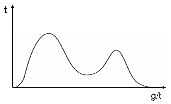
In statistics, a multimodal distribution is a probability distribution with more than one mode. These appear as distinct peaks (local maxima) in the probability density function, as shown in Figures 1 and 2. Categorical, continuous, and discrete data can all form multimodal distributions. Among univariate analyses, multimodal distributions are commonly bimodal.

Terminology

When the two modes are unequal the larger mode is known as the major mode and the other as the minor mode. The least frequent value between the modes is known as the antimode. The difference between the major and minor modes is known as the amplitude. In time series the major mode is called the acrophase and the antimode the batiphase.

Galtung's classification

Galtung introduced a classification system (AJUS) for distributions:

*A: unimodal distribution – peak in the middle
*J: unimodal – peak at either end
*U: bimodal – peaks at both ends
*S: bimodal or multimodal – multiple peaks

This classification has since been modified slightly:

*J: (modified) – peak on right
*L: unimodal – peak on left
*F: no peak (flat)

Under this classification bimodal distributions are classified as type S or U.

Examples

Bimodal distributions occur both in mathematics and in the natural sciences.

Probability distributions

Important bimodal distributions include the arcsine distribution and the beta distribution (iff both parameters are less than 1). Others include the U-quadratic distribution.

The ratio of two normal distributions is also bimodally distributed. Let

: $R = \frac$

where ''a'' and ''b'' are constant and ''x'' and ''y'' are distributed as normal variables with a mean of 0 and a standard deviation of 1. ''R'' has a known density that can be expressed as a confluent hypergeometric function.

The distribution of the reciprocal of a ''t'' distributed random variable is bimodal when the degrees of freedom are more than one. Similarly the reciprocal of a normally distributed variable is also bimodally distributed.

A ''t'' statistic generated from data set drawn from a Cauchy distribution is bimodal.

Occurrences in nature

Examples of variables with bimodal distributions include the time between eruptions of certain geysers, the color of galaxies, the size of worker weaver ants, the age of incidence of Hodgkin's lymphoma, the speed of inactivation of the drug isoniazid in US adults, the absolute magnitude of novae, and the circadian activity patterns of those crepuscular animals that are active both in morning and evening twilight. In fishery science multimodal length distributions reflect the different year classes and can thus be used for age distribution- and growth estimates of the fish population. Sediments are usually distributed in a bimodal fashion. When sampling mining galleries crossing either the host rock and the mineralized veins, the distribution of geochemical variables would be bimodal. Bimodal distributions are also seen in traffic analysis, where traffic peaks in during the AM rush hour and then again in the PM rush hour. This phenomenon is also seen in daily water distribution, as water demand, in the form of showers, cooking, and toilet use, generally peak in the morning and evening periods.

Econometrics

In econometric models, the parameters may be bimodally distributed.

Origins

Mathematical

A bimodal distribution most commonly arises as a mixture of two different unimodal distributions (i.e. distributions having only one mode). In other words, the bimodally distributed random variable X is defined as $Y$ with probability $\alpha$ or $Z$ with probability $(1-\alpha),$ where ''Y'' and ''Z'' are unimodal random variables and $0 < \alpha < 1$ is a mixture coefficient.

Mixtures with two distinct components need not be bimodal and two component mixtures of unimodal component densities can have more than two modes. There is no immediate connection between the number of components in a mixture and the number of modes of the resulting density.

Particular distributions

Bimodal distributions, despite their frequent occurrence in data sets, have only rarely been studied. This may be because of the difficulties in estimating their parameters either with frequentist or Bayesian methods. Among those that have been studied are

* Bimodal exponential distribution.
* Alpha-skew-normal distribution.
* Bimodal skew-symmetric normal distribution.
* A mixture of Conway-Maxwell-Poisson distributions has been fitted to bimodal count data.

Bimodality also naturally arises in the cusp catastrophe distribution.

Biology

In biology five factors are known to contribute to bimodal distributions of population sizes:

*the initial distribution of individual sizes
*the distribution of growth rates among the individuals
*the size and time dependence of the growth rate of each individual
* mortality rates that may affect each size class differently
* the DNA methylation in human and mouse genome.

The bimodal distribution of sizes of weaver ant workers arises due to existence of two distinct classes of workers, namely major workers and minor workers.

The distribution of fitness effects of mutations for both whole genomes and individual genes is also frequently found to be bimodal with most mutations being either neutral or lethal with relatively few having intermediate effect.

General properties

A mixture of two unimodal distributions with differing means is not necessarily bimodal. The combined distribution of heights of men and women is sometimes used as an example of a bimodal distribution, but in fact the difference in mean heights of men and women is too small relative to their standard deviations to produce bimodality.

Bimodal distributions have the peculiar property that – unlike the unimodal distributions – the mean may be a more robust sample estimator than the median. This is clearly the case when the distribution is U shaped like the arcsine distribution. It may not be true when the distribution has one or more long tails.

Moments of mixtures

Let

: $f( x ) = p g_1( x ) + ( 1 - p ) g_2( x ) \,$

where ''g''_''i'' is a probability distribution and ''p'' is the mixing parameter.

The moments of ''f''(''x'') are

: $\mu = p \mu_1 + ( 1 - p ) \mu_2$

: \nu_2 = p \sigma_1^2 + \delta_1^2 + ( 1 - p ) \sigma_2^2 + \delta_2^2 /math>

: \nu_3 = p S_1 \sigma_1^3 + 3 \delta_1 \sigma_1^2 + \delta_1^3 + ( 1 - p ) S_2 \sigma_2^3 + 3 \delta_2 \sigma_2^2 + \delta_2^3

: \nu_4 = p K_1 \sigma_1^4 + 4 S_1 \delta_1 \sigma_1^3 + 6 \delta_1^2 \sigma_1^2 + \delta_1^4 + ( 1 - p ) K_2 \sigma_2^4 + 4 S_2 \delta_2 \sigma_2^3 + 6 \delta_2^2 \sigma_2^2 + \delta_2^4 /math>

where
: $\mu = \int x f( x ) \, dx$

: $\delta_i = \mu_i - \mu$

: $\nu_r = \int ( x - \mu )^r f( x ) \, dx$

and ''S''_''i'' and ''K''_''i'' are the skewness and kurtosis of the ''i''^th distribution.

Mixture of two normal distributions

It is not uncommon to encounter situations where an investigator believes that the data comes from a mixture of two normal distributions. Because of this, this mixture has been studied in some detail.

A mixture of two normal distributions has five parameters to estimate: the two means, the two variances and the mixing parameter. A mixture of two normal distributions with equal standard deviations is bimodal only if their means differ by at least twice the common standard deviation. Estimates of the parameters is simplified if the variances can be assumed to be equal (the homoscedastic case).

If the means of the two normal distributions are equal, then the combined distribution is unimodal. Conditions for unimodality of the combined distribution were derived by Eisenberger. Necessary and sufficient conditions for a mixture of normal distributions to be bimodal have been identified by Ray and Lindsay.

A mixture of two approximately equal mass normal distributions has a negative kurtosis since the two modes on either side of the center of mass effectively reduces the tails of the distribution.

A mixture of two normal distributions with highly unequal mass has a positive kurtosis since the smaller distribution lengthens the tail of the more dominant normal distribution.

Mixtures of other distributions require additional parameters to be estimated.

Tests for unimodality

*When the components of the mixture have equal variances the mixture is unimodal if and only if

: $d \le 1$

or

: $\left\vert \log( 1 - p ) - \log( p ) \right\vert \ge 2 \log( d - \sqrt ) + 2d \sqrt ,$

where ''p'' is the mixing parameter and

: $d = \frac,$

and where ''μ''₁ and ''μ''₂ are the means of the two normal distributions and ''σ'' is their standard deviation.

*The following test for the case ''p'' = 1/2 was described by Schilling ''et al''. Let

:$r = \frac .$

The separation factor (''S'') is

:$S = \frac .$

If the variances are equal then ''S'' = 1. The mixture density is unimodal if and only if

:$, \mu_1 - \mu_2 , < S , \sigma_1 + \sigma_2 , .$

*A sufficient condition for unimodality is

:$, \mu_1-\mu_2, \le2\min (\sigma_1,\sigma_2).$

*If the two normal distributions have equal standard deviations $\sigma,$ a sufficient condition for unimodality is

:$, \mu _1-\mu_2, \le 2\sigma \sqrt.$

Summary statistics

Bimodal distributions are a commonly used example of how summary statistics such as the mean, median, and standard deviation can be deceptive when used on an arbitrary distribution. For example, in the distribution in Figure 1, the mean and median would be about zero, even though zero is not a typical value. The standard deviation is also larger than deviation of each normal distribution.

Although several have been suggested, there is no presently generally agreed summary statistic (or set of statistics) to quantify the parameters of a general bimodal distribution. For a mixture of two normal distributions the means and standard deviations along with the mixing parameter (the weight for the combination) are usually used – a total of five parameters.

Ashman's D

A statistic that may be useful is Ashman's D:

: $D = (2^\frac) \frac$

where ''μ''₁, ''μ''₂ are the means and ''σ''₁ ''σ''₂ are the standard deviations.

For a mixture of two normal distributions ''D'' > 2 is required for a clean separation of the distributions.

van der Eijk's A

This measure is a weighted average of the degree of agreement the frequency distribution. ''A'' ranges from -1 (perfect bimodality) to +1 (perfect unimodality). It is defined as

: $A = U ( 1 - \frac )$

where ''U'' is the unimodality of the distribution, ''S'' the number of categories that have nonzero frequencies and ''K'' the total number of categories.

The value of U is 1 if the distribution has any of the three following characteristics:

* all responses are in a single category
* the responses are evenly distributed among all the categories
* the responses are evenly distributed among two or more contiguous categories, with the other categories with zero responses

With distributions other than these the data must be divided into 'layers'. Within a layer the responses are either equal or zero. The categories do not have to be contiguous. A value for ''A'' for each layer (''A''_i) is calculated and a weighted average for the distribution is determined. The weights (''w''_i) for each layer are the number of responses in that layer. In symbols

:$A_ = \sum w_i A_i$

A uniform distribution has ''A'' = 0: when all the responses fall into one category ''A'' = +1.

One theoretical problem with this index is that it assumes that the intervals are equally spaced. This may limit its applicability.

Bimodal separation

This index assumes that the distribution is a mixture of two normal distributions with means (''μ''₁ and ''μ''₂) and standard deviations (''σ''₁ and ''σ''₂):

: $S = \frac$

Bimodality coefficient

Sarle's bimodality coefficient ''b'' is

: $\beta = \frac$

where ''γ'' is the skewness and ''κ'' is the kurtosis. The kurtosis is here defined to be the standardised fourth moment around the mean. The value of ''b'' lies between 0 and 1. The logic behind this coefficient is that a bimodal distribution with light tails will have very low kurtosis, an asymmetric character, or both – all of which increase this coefficient.

The formula for a finite sample isSAS Institute Inc. (2012). SAS/STAT 12.1 user’s guide. Cary, NC: Author.

: $b = \frac$

where ''n'' is the number of items in the sample, ''g'' is the sample skewness and ''k'' is the sample excess kurtosis.

The value of ''b'' for the uniform distribution is 5/9. This is also its value for the exponential distribution. Values greater than 5/9 may indicate a bimodal or multimodal distribution, though corresponding values can also result for heavily skewed unimodal distributions. The maximum value (1.0) is reached only by a Bernoulli distribution with only two distinct values or the sum of two different Dirac delta functions (a bi-delta distribution).

The distribution of this statistic is unknown. It is related to a statistic proposed earlier by Pearson – the difference between the kurtosis and the square of the skewness (''vide infra'').

Bimodality amplitude

This is defined as

: $A_B = \frac$

where ''A''₁ is the amplitude of the smaller peak and ''A''_an is the amplitude of the antimode.

''A''_B is always < 1. Larger values indicate more distinct peaks.

Bimodal ratio

This is the ratio of the left and right peaks. Mathematically

: $R = \frac$

where ''A''_l and ''A''_r are the amplitudes of the left and right peaks respectively.

Bimodality parameter

This parameter (''B'') is due to Wilcock.

: $B = \sqrt \sum P_i$

where ''A''_l and ''A''_r are the amplitudes of the left and right peaks respectively and ''P''_''i'' is the logarithm taken to the base 2 of the proportion of the distribution in the i^th interval. The maximal value of the ''ΣP'' is 1 but the value of ''B'' may be greater than this.

To use this index, the log of the values are taken. The data is then divided into interval of width Φ whose value is log 2. The width of the peaks are taken to be four times 1/4Φ centered on their maximum values.

Bimodality indices

;Wang's index

The bimodality index proposed by Wang ''et al'' assumes that the distribution is a sum of two normal distributions with equal variances but differing means. It is defined as follows:

: $\delta = \frac$

where ''μ''₁, ''μ''₂ are the means and ''σ'' is the common standard deviation.

: $BI = \delta \sqrt$

where ''p'' is the mixing parameter.

;Sturrock's index

A different bimodality index has been proposed by Sturrock.

This index (''B'') is defined as

: B = \frac \left \left( \sum_1^N \cos ( 2 \pi m \gamma ) \right)^2 + \left( \sum_1^N \sin ( 2 \pi m \gamma ) \right)^2 \right

When ''m'' = 2 and ''γ'' is uniformly distributed, ''B'' is exponentially distributed.

This statistic is a form of periodogram. It suffers from the usual problems of estimation and spectral leakage common to this form of statistic.

;de Michele and Accatino's index

Another bimodality index has been proposed by de Michele and Accatino. Their index (''B'') is

: $B = , \mu - \mu_M ,$

where ''μ'' is the arithmetic mean of the sample and

: $\mu_M = \frac$

where ''m''_''i'' is number of data points in the ''i''^th bin, ''x''_''i'' is the center of the ''i''^th bin and ''L'' is the number of bins.

The authors suggested a cut off value of 0.1 for ''B'' to distinguish between a bimodal (''B'' > 0.1)and unimodal (''B'' < 0.1) distribution. No statistical justification was offered for this value.

;Sambrook Smith's index

A further index (''B'') has been proposed by Sambrook Smith ''et al''

$B = , \phi_2 - \phi_1 , \frac$

where ''p''₁ and ''p''₂ are the proportion contained in the primary (that with the greater amplitude) and secondary (that with the lesser amplitude) mode and ''φ''₁ and ''φ''₂ are the ''φ''-sizes of the primary and secondary mode. The ''φ''-size is defined as minus one times the log of the data size taken to the base 2. This transformation is commonly used in the study of sediments.

The authors recommended a cut off value of 1.5 with B being greater than 1.5 for a bimodal distribution and less than 1.5 for a unimodal distribution. No statistical justification for this value was given.

;Otsu's method

Otsu's method for finding a threshold for separation between two modes relies on minimizing the quantity
$\frac$
where ''n''_''i'' is the number of data points in the ''i''^th subpopulation, ''σ''_''i''² is the variance of the ''i''^th subpopulation, ''m'' is the total size of the sample and ''σ''² is the sample variance. Some researchers (particularly in the field of digital image processing) have applied this quantity more broadly as an index for detecting bimodality, with a small value indicating a more bimodal distribution.

Statistical tests

A number of tests are available to determine if a data set is distributed in a bimodal (or multimodal) fashion.

Graphical methods

In the study of sediments, particle size is frequently bimodal. Empirically, it has been found useful to plot the frequency against the log( size ) of the particles. This usually gives a clear separation of the particles into a bimodal distribution. In geological applications the logarithm is normally taken to the base 2. The log transformed values are referred to as phi (Φ) units. This system is known as the Krumbein (or phi) scale.

An alternative method is to plot the log of the particle size against the cumulative frequency. This graph will usually consist two reasonably straight lines with a connecting line corresponding to the antimode.

;Statistics

Approximate values for several statistics can be derived from the graphic plots.

: $\mathit = \frac$

: $\mathit = \frac + \frac$

: $\mathit = \frac + \frac$

: $\mathit = \frac$

where ''Mean'' is the mean, ''StdDev'' is the standard deviation, ''Skew'' is the skewness, ''Kurt'' is the kurtosis and ''φ''_x is the value of the variate ''φ'' at the ''x''^th percentage of the distribution.

Unimodal vs. bimodal distribution

Pearson in 1894 was the first to devise a procedure to test whether a distribution could be resolved into two normal distributions. This method required the solution of a ninth order polynomial. In a subsequent paper Pearson reported that for any distribution skewness² + 1 < kurtosis. Later Pearson showed that

: $b_2 - b_1 \ge 1$

where ''b''₂ is the kurtosis and ''b''₁ is the square of the skewness. Equality holds only for the two point Bernoulli distribution or the sum of two different Dirac delta functions. These are the most extreme cases of bimodality possible. The kurtosis in both these cases is 1. Since they are both symmetrical their skewness is 0 and the difference is 1.

Baker proposed a transformation to convert a bimodal to a unimodal distribution.

Several tests of unimodality versus bimodality have been proposed: Haldane suggested one based on second central differences. Larkin later introduced a test based on the F test; Benett created one based on Fisher's G test. Tokeshi has proposed a fourth test. A test based on a likelihood ratio has been proposed by Holzmann and Vollmer.

A method based on the score and Wald tests has been proposed. This method can distinguish between unimodal and bimodal distributions when the underlying distributions are known.

Antimode tests

Statistical tests for the antimode are known.

;Otsu's method

Otsu's method is commonly employed in computer graphics to determine the optimal separation between two distributions.

General tests

To test if a distribution is other than unimodal, several additional tests have been devised: the bandwidth test, the dip test, the excess mass test, the MAP test, the mode existence test, the runt test, the span test, and the saddle test.

An implementation of the dip test is available for the R programming language. The p-values for the dip statistic values range between 0 and 1. P-values less than 0.05 indicate significant multimodality and p-values greater than 0.05 but less than 0.10 suggest multimodality with marginal significance.

Silverman's test

Silverman introduced a bootstrap method for the number of modes. The test uses a fixed bandwidth which reduces the power of the test and its interpretability. Under smoothed densities may have an excessive number of modes whose count during bootstrapping is unstable.

Bajgier-Aggarwal test

Bajgier and Aggarwal have proposed a test based on the kurtosis of the distribution.

Special cases

Additional tests are available for a number of special cases:

;Mixture of two normal distributions

A study of a mixture density of two normal distributions data found that separation into the two normal distributions was difficult unless the means were separated by 4–6 standard deviations.

In astronomy the Kernel Mean Matching algorithm is used to decide if a data set belongs to a single normal distribution or to a mixture of two normal distributions.

;Beta-normal distribution

This distribution is bimodal for certain values of is parameters. A test for these values has been described.

Parameter estimation and fitting curves

Assuming that the distribution is known to be bimodal or has been shown to be bimodal by one or more of the tests above, it is frequently desirable to fit a curve to the data. This may be difficult.

Bayesian methods may be useful in difficult cases.

Software

;Two normal distributions

A package for R is available for testing for bimodality. This package assumes that the data are distributed as a sum of two normal distributions. If this assumption is not correct the results may not be reliable. It also includes functions for fitting a sum of two normal distributions to the data.

Assuming that the distribution is a mixture of two normal distributions then the expectation-maximization algorithm may be used to determine the parameters. Several programmes are available for this including Cluster, and the R package nor1mix.

;Other distributions

The mixtools package available for R can test for and estimate the parameters of a number of different distributions. A package for a mixture of two right-tailed gamma distributions is available.

Several other packages for R are available to fit mixture models; these include flexmix, mcclust, agrmt, and mixdist.

The statistical programming language SAS can also fit a variety of mixed distributions with the PROC FREQ procedure.

Example software application

The CumFreqA CumFreq, free program for fitting of probability distributions to a data set. On line

program for the fitting of composite probability distributions to a data set (X) can divide the set into two parts with a different distribution. The figure shows an example of a double generalized mirrored Gumbel distribution as in distribution fitting with cumulative distribution function (CDF) equations:

X < 8.10 : CDF = 1 - expexp X > 8.10 : CDF = 1 - expexp

See also

* Overdispersion

References

{{ProbDistributions

Continuous distributions