HOME

TheInfoList


OR:

In
probability theory Probability theory is the branch of mathematics concerned with probability. Although there are several different probability interpretations, probability theory treats the concept in a rigorous mathematical manner by expressing it through a set ...
and statistics, the beta distribution is a family of continuous probability distributions defined on the interval
, 1 The comma is a punctuation mark that appears in several variants in different languages. It has the same shape as an apostrophe or single closing quotation mark () in many typefaces, but it differs from them in being placed on the baseline o ...
in terms of two positive
parameters A parameter (), generally, is any characteristic that can help in defining or classifying a particular system (meaning an event, project, object, situation, etc.). That is, a parameter is an element of a system that is useful, or critical, when ...
, denoted by ''alpha'' (''α'') and ''beta'' (''β''), that appear as exponents of the random variable and control the
shape A shape or figure is a graphical representation of an object or its external boundary, outline, or external surface, as opposed to other properties such as color, texture, or material type. A plane shape or plane figure is constrained to lie ...
of the distribution. The beta distribution has been applied to model the behavior of random variables limited to intervals of finite length in a wide variety of disciplines. The beta distribution is a suitable model for the random behavior of percentages and proportions. In Bayesian inference, the beta distribution is the conjugate prior probability distribution for the
Bernoulli Bernoulli can refer to: People *Bernoulli family of 17th and 18th century Swiss mathematicians: ** Daniel Bernoulli (1700–1782), developer of Bernoulli's principle **Jacob Bernoulli (1654–1705), also known as Jacques, after whom Bernoulli numbe ...
, binomial,
negative binomial In probability theory and statistics, the negative binomial distribution is a discrete probability distribution that models the number of failures in a sequence of independent and identically distributed Bernoulli trials before a specified (non-r ...
and geometric distributions. The formulation of the beta distribution discussed here is also known as the beta distribution of the first kind, whereas ''beta distribution of the second kind'' is an alternative name for the
beta prime distribution In probability theory and statistics, the beta prime distribution (also known as inverted beta distribution or beta distribution of the second kindJohnson et al (1995), p 248) is an absolutely continuous probability distribution. Definitions ...
. The generalization to multiple variables is called a
Dirichlet distribution In probability and statistics, the Dirichlet distribution (after Peter Gustav Lejeune Dirichlet), often denoted \operatorname(\boldsymbol\alpha), is a family of continuous multivariate probability distributions parameterized by a vector \bold ...
.


Definitions


Probability density function
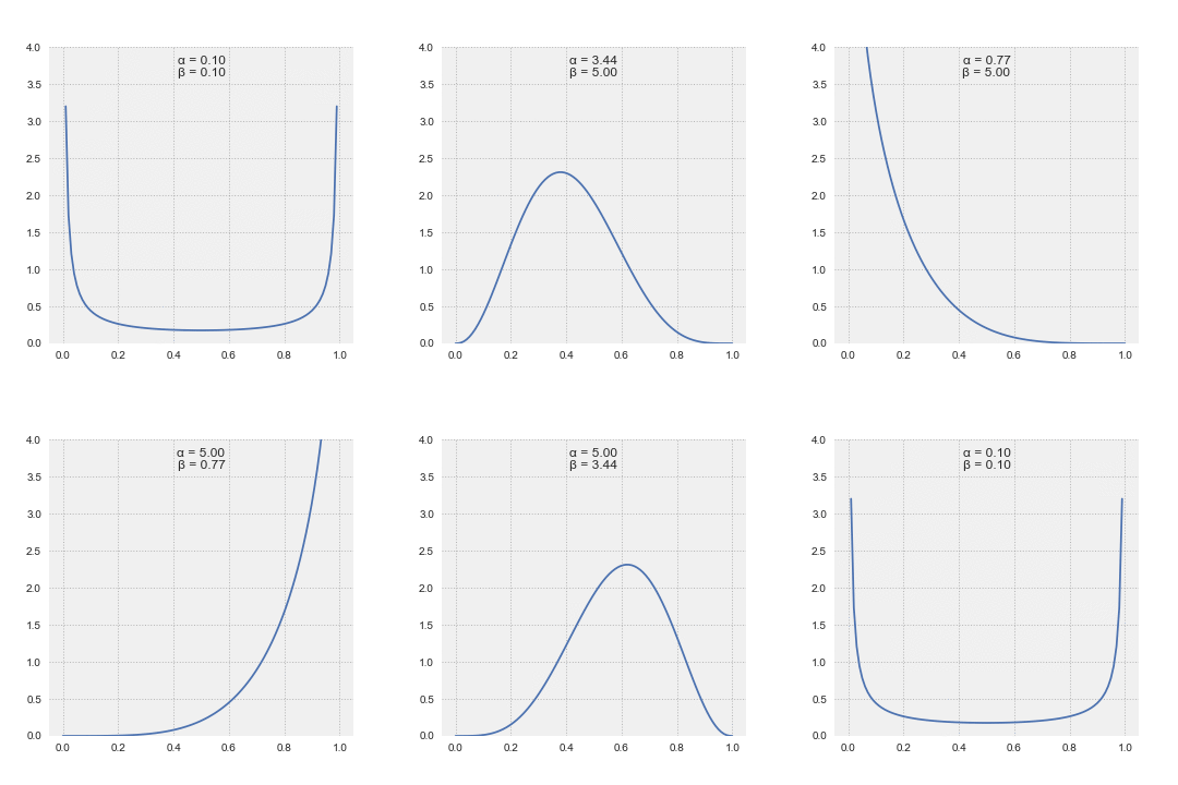
The
probability density function In probability theory, a probability density function (PDF), or density of a continuous random variable, is a function whose value at any given sample (or point) in the sample space (the set of possible values taken by the random variable) ca ...
(PDF) of the beta distribution, for , and shape parameters ''α'', ''β'' > 0, is a
power function Exponentiation is a mathematical operation, written as , involving two numbers, the '' base'' and the ''exponent'' or ''power'' , and pronounced as " (raised) to the (power of) ". When is a positive integer, exponentiation corresponds to re ...
of the variable ''x'' and of its
reflection Reflection or reflexion may refer to: Science and technology * Reflection (physics), a common wave phenomenon ** Specular reflection, reflection from a smooth surface *** Mirror image, a reflection in a mirror or in water ** Signal reflection, in ...
as follows: : \begin f(x;\alpha,\beta) & = \mathrm\cdot x^(1-x)^ \\ pt& = \frac \\ pt& = \frac\, x^(1-x)^ \\ pt& = \frac x^(1-x)^ \end where Γ(''z'') is the
gamma function In mathematics, the gamma function (represented by , the capital letter gamma from the Greek alphabet) is one commonly used extension of the factorial function to complex numbers. The gamma function is defined for all complex numbers except ...
. The
beta function In mathematics, the beta function, also called the Euler integral of the first kind, is a special function that is closely related to the gamma function and to binomial coefficients. It is defined by the integral : \Beta(z_1,z_2) = \int_0^1 t^( ...
, \Beta, is a
normalization constant The concept of a normalizing constant arises in probability theory and a variety of other areas of mathematics. The normalizing constant is used to reduce any probability function to a probability density function with total probability of one. ...
to ensure that the total probability is 1. In the above equations ''x'' is a realization—an observed value that actually occurred—of a
random process In probability theory and related fields, a stochastic () or random process is a mathematical object usually defined as a family of random variables. Stochastic processes are widely used as mathematical models of systems and phenomena that appea ...
 ''X''. This definition includes both ends and , which is consistent with definitions for other continuous distributions supported on a bounded interval which are special cases of the beta distribution, for example the arcsine distribution, and consistent with several authors, like N. L. Johnson and S. Kotz. However, the inclusion of and does not work for ; accordingly, several other authors, including W. Feller, choose to exclude the ends and , (so that the two ends are not actually part of the domain of the density function) and consider instead . Several authors, including N. L. Johnson and S. Kotz, use the symbols ''p'' and ''q'' (instead of ''α'' and ''β'') for the shape parameters of the beta distribution, reminiscent of the symbols traditionally used for the parameters of the
Bernoulli distribution In probability theory and statistics, the Bernoulli distribution, named after Swiss mathematician Jacob Bernoulli,James Victor Uspensky: ''Introduction to Mathematical Probability'', McGraw-Hill, New York 1937, page 45 is the discrete probabi ...
, because the beta distribution approaches the Bernoulli distribution in the limit when both shape parameters ''α'' and ''β'' approach the value of zero. In the following, a random variable ''X'' beta-distributed with parameters ''α'' and ''β'' will be denoted by: :X \sim \operatorname(\alpha, \beta) Other notations for beta-distributed random variables used in the statistical literature are X \sim \mathcale(\alpha, \beta) and X \sim \beta_.


Cumulative distribution function

The cumulative distribution function is :F(x;\alpha,\beta) = \frac = I_x(\alpha,\beta) where \Beta(x;\alpha,\beta) is the incomplete beta function and I_x(\alpha,\beta) is the regularized incomplete beta function.


Alternative parameterizations


Two parameters


=Mean and sample size

= The beta distribution may also be reparameterized in terms of its mean ''μ'' and the sum of the two shape parameters ( p. 83). Denoting by αPosterior and βPosterior the shape parameters of the posterior beta distribution resulting from applying Bayes theorem to a binomial likelihood function and a prior probability, the interpretation of the addition of both shape parameters to be sample size = ''ν'' = ''α''·Posterior + ''β''·Posterior is only correct for the Haldane prior probability Beta(0,0). Specifically, for the Bayes (uniform) prior Beta(1,1) the correct interpretation would be sample size = ''α''·Posterior + ''β'' Posterior − 2, or ''ν'' = (sample size) + 2. For sample size much larger than 2, the difference between these two priors becomes negligible. (See section Bayesian inference for further details.) ν = α + β is referred to as the "sample size" of a Beta distribution, but one should remember that it is, strictly speaking, the "sample size" of a binomial likelihood function only when using a Haldane Beta(0,0) prior in Bayes theorem. This parametrization may be useful in Bayesian parameter estimation. For example, one may administer a test to a number of individuals. If it is assumed that each person's score (0 ≤ ''θ'' ≤ 1) is drawn from a population-level Beta distribution, then an important statistic is the mean of this population-level distribution. The mean and sample size parameters are related to the shape parameters α and β via : ''α'' = ''μν'', ''β'' = (1 − ''μ'')''ν'' Under this parametrization, one may place an
uninformative prior In Bayesian statistical inference, a prior probability distribution, often simply called the prior, of an uncertain quantity is the probability distribution that would express one's beliefs about this quantity before some evidence is taken into ...
probability over the mean, and a vague prior probability (such as an exponential or gamma distribution) over the positive reals for the sample size, if they are independent, and prior data and/or beliefs justify it.


=Mode and concentration

=
Concave Concave or concavity may refer to: Science and technology * Concave lens * Concave mirror Mathematics * Concave function, the negative of a convex function * Concave polygon, a polygon which is not convex * Concave set * The concavity of a ...
beta distributions, which have \alpha,\beta>1, can be parametrized in terms of mode and "concentration". The mode, \omega=\frac, and concentration, \kappa = \alpha + \beta, can be used to define the usual shape parameters as follows: :\begin \alpha &= \omega (\kappa - 2) + 1\\ \beta &= (1 - \omega)(\kappa - 2) + 1 \end For the mode, 0<\omega<1, to be well-defined, we need \alpha,\beta>1, or equivalently \kappa>2. If instead we define the concentration as c=\alpha+\beta-2, the condition simplifies to c>0 and the beta density at \alpha=1+c\omega and \beta=1+c(1-\omega) can be written as: : f(x;\omega,c) = \frac where c directly scales the sufficient statistics, \log(x) and \log(1-x). Note also that in the limit, c\to0, the distribution becomes flat.


=Mean and variance

= Solving the system of (coupled) equations given in the above sections as the equations for the mean and the variance of the beta distribution in terms of the original parameters ''α'' and ''β'', one can express the ''α'' and ''β'' parameters in terms of the mean (''μ'') and the variance (var): : \begin \nu &= \alpha + \beta = \frac-1, \text\nu =(\alpha + \beta) >0,\text\text< \mu(1-\mu)\\ \alpha&= \mu \nu =\mu \left(\frac-1\right), \text \text< \mu(1-\mu)\\ \beta &= (1 - \mu) \nu = (1 - \mu)\left(\frac-1\right), \text\text< \mu(1-\mu). \end This parametrization of the beta distribution may lead to a more intuitive understanding than the one based on the original parameters ''α'' and ''β''. For example, by expressing the mode, skewness, excess kurtosis and differential entropy in terms of the mean and the variance:


Four parameters

A beta distribution with the two shape parameters α and β is supported on the range ,1or (0,1). It is possible to alter the location and scale of the distribution by introducing two further parameters representing the minimum, ''a'', and maximum ''c'' (''c'' > ''a''), values of the distribution, by a linear transformation substituting the non-dimensional variable ''x'' in terms of the new variable ''y'' (with support 'a'',''c''or (''a'',''c'')) and the parameters ''a'' and ''c'': :y = x(c-a) + a, \textx = \frac. The
probability density function In probability theory, a probability density function (PDF), or density of a continuous random variable, is a function whose value at any given sample (or point) in the sample space (the set of possible values taken by the random variable) ca ...
of the four parameter beta distribution is equal to the two parameter distribution, scaled by the range (''c''-''a''), (so that the total area under the density curve equals a probability of one), and with the "y" variable shifted and scaled as follows: ::f(y; \alpha, \beta, a, c) = \frac =\frac=\frac. That a random variable ''Y'' is Beta-distributed with four parameters α, β, ''a'', and ''c'' will be denoted by: :Y \sim \operatorname(\alpha, \beta, a, c). Some measures of central location are scaled (by (''c''-''a'')) and shifted (by ''a''), as follows: : \begin \mu_Y &= \mu_X(c-a) + a = \left(\frac\right)(c-a) + a = \frac \\ \text(Y) &=\text(X)(c-a) + a = \left(\frac\right)(c-a) + a = \frac\ ,\qquad \text \alpha, \beta>1 \\ \text(Y) &= \text(X)(c-a) + a = \left (I_^(\alpha,\beta) \right )(c-a)+a \\ \end Note: the geometric mean and harmonic mean cannot be transformed by a linear transformation in the way that the mean, median and mode can. The shape parameters of ''Y'' can be written in term of its mean and variance as : \begin \alpha &= \frac \\ \beta &= -\frac \\ \end The statistical dispersion measures are scaled (they do not need to be shifted because they are already centered on the mean) by the range (c-a), linearly for the mean deviation and nonlinearly for the variance: ::\text(Y)= ::(\text(X))(c-a) =\frac(c-a) :: \text(Y) =\text(X)(c-a)^2 =\frac. Since the
skewness In probability theory and statistics, skewness is a measure of the asymmetry of the probability distribution of a real-valued random variable about its mean. The skewness value can be positive, zero, negative, or undefined. For a unimodal ...
and
excess kurtosis In probability theory and statistics, kurtosis (from el, κυρτός, ''kyrtos'' or ''kurtos'', meaning "curved, arching") is a measure of the "tailedness" of the probability distribution of a real-valued random variable. Like skewness, kurtosi ...
are non-dimensional quantities (as moments centered on the mean and normalized by the standard deviation), they are independent of the parameters ''a'' and ''c'', and therefore equal to the expressions given above in terms of ''X'' (with support ,1or (0,1)): :: \text(Y) =\text(X) = \frac. :: \text(Y) =\text(X)=\frac


Properties


Measures of central tendency


Mode

The
mode Mode ( la, modus meaning "manner, tune, measure, due measure, rhythm, melody") may refer to: Arts and entertainment * '' MO''D''E (magazine)'', a defunct U.S. women's fashion magazine * ''Mode'' magazine, a fictional fashion magazine which is ...
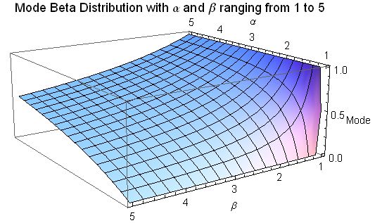
of a Beta distributed random variable ''X'' with ''α'', ''β'' > 1 is the most likely value of the distribution (corresponding to the peak in the PDF), and is given by the following expression: :\frac . When both parameters are less than one (''α'', ''β'' < 1), this is the anti-mode: the lowest point of the probability density curve. Letting ''α'' = ''β'', the expression for the mode simplifies to 1/2, showing that for ''α'' = ''β'' > 1 the mode (resp. anti-mode when ), is at the center of the distribution: it is symmetric in those cases. See
Shapes A shape or figure is a graphical representation of an object or its external boundary, outline, or external surface, as opposed to other properties such as color, texture, or material type. A plane shape or plane figure is constrained to lie o ...
section in this article for a full list of mode cases, for arbitrary values of ''α'' and ''β''. For several of these cases, the maximum value of the density function occurs at one or both ends. In some cases the (maximum) value of the density function occurring at the end is finite. For example, in the case of ''α'' = 2, ''β'' = 1 (or ''α'' = 1, ''β'' = 2), the density function becomes a right-triangle distribution which is finite at both ends. In several other cases there is a singularity at one end, where the value of the density function approaches infinity. For example, in the case ''α'' = ''β'' = 1/2, the Beta distribution simplifies to become the arcsine distribution. There is debate among mathematicians about some of these cases and whether the ends (''x'' = 0, and ''x'' = 1) can be called ''modes'' or not. * Whether the ends are part of the domain of the density function * Whether a singularity can ever be called a ''mode'' * Whether cases with two maxima should be called ''bimodal''


Median

The median of the beta distribution is the unique real number x = I_^(\alpha,\beta) for which the regularized incomplete beta function I_x(\alpha,\beta) = \tfrac . There is no general
closed-form expression In mathematics, a closed-form expression is a mathematical expression that uses a finite number of standard operations. It may contain constants, variables, certain well-known operations (e.g., + − × ÷), and functions (e.g., ''n''th ro ...
for the median of the beta distribution for arbitrary values of ''α'' and ''β''.
Closed-form expression In mathematics, a closed-form expression is a mathematical expression that uses a finite number of standard operations. It may contain constants, variables, certain well-known operations (e.g., + − × ÷), and functions (e.g., ''n''th ro ...
s for particular values of the parameters ''α'' and ''β'' follow: * For symmetric cases ''α'' = ''β'', median = 1/2. * For ''α'' = 1 and ''β'' > 0, median =1-2^ (this case is the mirror-image of the power function ,1distribution) * For ''α'' > 0 and ''β'' = 1, median = 2^ (this case is the power function ,1distribution) * For ''α'' = 3 and ''β'' = 2, median = 0.6142724318676105..., the real solution to the
quartic equation In mathematics, a quartic equation is one which can be expressed as a ''quartic function'' equaling zero. The general form of a quartic equation is :ax^4+bx^3+cx^2+dx+e=0 \, where ''a'' ≠ 0. The quartic is the highest order polynomi ...
1 − 8''x''3 + 6''x''4 = 0, which lies in ,1 * For ''α'' = 2 and ''β'' = 3, median = 0.38572756813238945... = 1−median(Beta(3, 2)) The following are the limits with one parameter finite (non-zero) and the other approaching these limits: : \begin \lim_ \text= \lim_ \text = 1,\\ \lim_ \text= \lim_ \text = 0. \end A reasonable approximation of the value of the median of the beta distribution, for both α and β greater or equal to one, is given by the formula :\text \approx \frac \text \alpha, \beta \ge 1. When α, β ≥ 1, the
relative error The approximation error in a data value is the discrepancy between an exact value and some '' approximation'' to it. This error can be expressed as an absolute error (the numerical amount of the discrepancy) or as a relative error (the absolute e ...
(the absolute error divided by the median) in this approximation is less than 4% and for both α ≥ 2 and β ≥ 2 it is less than 1%. The absolute error divided by the difference between the mean and the mode is similarly small:
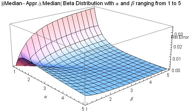
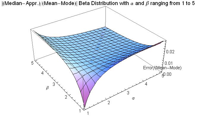
Mean

The expected value (mean) (''μ'') of a Beta distribution random variable ''X'' with two parameters ''α'' and ''β'' is a function of only the ratio ''β''/''α'' of these parameters: : \begin \mu = \operatorname &= \int_0^1 x f(x;\alpha,\beta)\,dx \\ &= \int_0^1 x \,\frac\,dx \\ &= \frac \\ &= \frac \end Letting in the above expression one obtains , showing that for the mean is at the center of the distribution: it is symmetric. Also, the following limits can be obtained from the above expression: : \begin \lim_ \mu = 1\\ \lim_ \mu = 0 \end Therefore, for ''β''/''α'' → 0, or for ''α''/''β'' → ∞, the mean is located at the right end, . For these limit ratios, the beta distribution becomes a one-point
degenerate distribution In mathematics, a degenerate distribution is, according to some, a probability distribution in a space with support only on a manifold of lower dimension, and according to others a distribution with support only at a single point. By the latter d ...
with a Dirac delta function spike at the right end, , with probability 1, and zero probability everywhere else. There is 100% probability (absolute certainty) concentrated at the right end, . Similarly, for ''β''/''α'' → ∞, or for ''α''/''β'' → 0, the mean is located at the left end, . The beta distribution becomes a 1-point
Degenerate distribution In mathematics, a degenerate distribution is, according to some, a probability distribution in a space with support only on a manifold of lower dimension, and according to others a distribution with support only at a single point. By the latter d ...
with a Dirac delta function spike at the left end, ''x'' = 0, with probability 1, and zero probability everywhere else. There is 100% probability (absolute certainty) concentrated at the left end, ''x'' = 0. Following are the limits with one parameter finite (non-zero) and the other approaching these limits: : \begin \lim_ \mu = \lim_ \mu = 1\\ \lim_ \mu = \lim_ \mu = 0 \end While for typical unimodal distributions (with centrally located modes, inflexion points at both sides of the mode, and longer tails) (with Beta(''α'', ''β'') such that ) it is known that the sample mean (as an estimate of location) is not as
robust Robustness is the property of being strong and healthy in constitution. When it is transposed into a system, it refers to the ability of tolerating perturbations that might affect the system’s functional body. In the same line ''robustness'' ca ...
as the sample median, the opposite is the case for uniform or "U-shaped" bimodal distributions (with Beta(''α'', ''β'') such that ), with the modes located at the ends of the distribution. As Mosteller and Tukey remark ( p. 207) "the average of the two extreme observations uses all the sample information. This illustrates how, for short-tailed distributions, the extreme observations should get more weight." By contrast, it follows that the median of "U-shaped" bimodal distributions with modes at the edge of the distribution (with Beta(''α'', ''β'') such that ) is not robust, as the sample median drops the extreme sample observations from consideration. A practical application of this occurs for example for
random walk In mathematics, a random walk is a random process that describes a path that consists of a succession of random steps on some mathematical space. An elementary example of a random walk is the random walk on the integer number line \mathbb Z ...
s, since the probability for the time of the last visit to the origin in a random walk is distributed as the arcsine distribution Beta(1/2, 1/2): the mean of a number of realizations of a random walk is a much more robust estimator than the median (which is an inappropriate sample measure estimate in this case).


Geometric mean

The logarithm of the geometric mean ''GX'' of a distribution with random variable ''X'' is the arithmetic mean of ln(''X''), or, equivalently, its expected value: :\ln G_X = \operatorname ln X/math> For a beta distribution, the expected value integral gives: :\begin \operatorname ln X&= \int_0^1 \ln x\, f(x;\alpha,\beta)\,dx \\ pt&= \int_0^1 \ln x \,\frac\,dx \\ pt&= \frac \, \int_0^1 \frac\,dx \\ pt&= \frac \frac \int_0^1 x^(1-x)^\,dx \\ pt&= \frac \frac \\ pt&= \frac \\ pt&= \frac - \frac \\ pt&= \psi(\alpha) - \psi(\alpha + \beta) \end where ''ψ'' is the
digamma function In mathematics, the digamma function is defined as the logarithmic derivative of the gamma function: :\psi(x)=\frac\ln\big(\Gamma(x)\big)=\frac\sim\ln-\frac. It is the first of the polygamma functions. It is strictly increasing and strict ...
. Therefore, the geometric mean of a beta distribution with shape parameters ''α'' and ''β'' is the exponential of the digamma functions of ''α'' and ''β'' as follows: :G_X =e^= e^ While for a beta distribution with equal shape parameters α = β, it follows that skewness = 0 and mode = mean = median = 1/2, the geometric mean is less than 1/2: . The reason for this is that the logarithmic transformation strongly weights the values of ''X'' close to zero, as ln(''X'') strongly tends towards negative infinity as ''X'' approaches zero, while ln(''X'') flattens towards zero as . Along a line , the following limits apply: : \begin &\lim_ G_X = 0 \\ &\lim_ G_X =\tfrac \end Following are the limits with one parameter finite (non-zero) and the other approaching these limits: : \begin \lim_ G_X = \lim_ G_X = 1\\ \lim_ G_X = \lim_ G_X = 0 \end The accompanying plot shows the difference between the mean and the geometric mean for shape parameters α and β from zero to 2. Besides the fact that the difference between them approaches zero as α and β approach infinity and that the difference becomes large for values of α and β approaching zero, one can observe an evident asymmetry of the geometric mean with respect to the shape parameters α and β. The difference between the geometric mean and the mean is larger for small values of α in relation to β than when exchanging the magnitudes of β and α. N. L.Johnson and S. Kotz suggest the logarithmic approximation to the digamma function ''ψ''(''α'') ≈ ln(''α'' − 1/2) which results in the following approximation to the geometric mean: :G_X \approx \frac\text \alpha, \beta > 1. Numerical values for the
relative error The approximation error in a data value is the discrepancy between an exact value and some '' approximation'' to it. This error can be expressed as an absolute error (the numerical amount of the discrepancy) or as a relative error (the absolute e ...
in this approximation follow: []; []; []; []; []; []; []; []. Similarly, one can calculate the value of shape parameters required for the geometric mean to equal 1/2. Given the value of the parameter ''β'', what would be the value of the other parameter, ''α'', required for the geometric mean to equal 1/2?. The answer is that (for ), the value of ''α'' required tends towards as . For example, all these couples have the same geometric mean of 1/2: [], [], [], [], [], [], []. The fundamental property of the geometric mean, which can be proven to be false for any other mean, is :G\left(\frac\right) = \frac This makes the geometric mean the only correct mean when averaging ''normalized'' results, that is results that are presented as ratios to reference values. This is relevant because the beta distribution is a suitable model for the random behavior of percentages and it is particularly suitable to the statistical modelling of proportions. The geometric mean plays a central role in maximum likelihood estimation, see section "Parameter estimation, maximum likelihood." Actually, when performing maximum likelihood estimation, besides the geometric mean ''GX'' based on the random variable X, also another geometric mean appears naturally: the geometric mean based on the linear transformation ––, the mirror-image of ''X'', denoted by ''G''(1−''X''): :G_ = e^ = e^ Along a line , the following limits apply: : \begin &\lim_ G_ =0 \\ &\lim_ G_ =\tfrac \end Following are the limits with one parameter finite (non-zero) and the other approaching these limits: : \begin \lim_ G_ = \lim_ G_ = 0\\ \lim_ G_ = \lim_ G_ = 1 \end It has the following approximate value: :G_ \approx \frac\text \alpha, \beta > 1. Although both ''G''''X'' and ''G''(1−''X'') are asymmetric, in the case that both shape parameters are equal , the geometric means are equal: ''G''''X'' = ''G''(1−''X''). This equality follows from the following symmetry displayed between both geometric means: :G_X (\Beta(\alpha, \beta) )=G_(\Beta(\beta, \alpha) ).


Harmonic mean

The inverse of the harmonic mean (''HX'') of a distribution with random variable ''X'' is the arithmetic mean of 1/''X'', or, equivalently, its expected value. Therefore, the harmonic mean (''HX'') of a beta distribution with shape parameters ''α'' and ''β'' is: : \begin H_X &= \frac \\ &=\frac \\ &=\frac \\ &= \frac\text \alpha > 1 \text \beta > 0 \\ \end The harmonic mean (''HX'') of a Beta distribution with ''α'' < 1 is undefined, because its defining expression is not bounded in
, 1 The comma is a punctuation mark that appears in several variants in different languages. It has the same shape as an apostrophe or single closing quotation mark () in many typefaces, but it differs from them in being placed on the baseline o ...
for shape parameter ''α'' less than unity. Letting ''α'' = ''β'' in the above expression one obtains :H_X = \frac, showing that for ''α'' = ''β'' the harmonic mean ranges from 0, for ''α'' = ''β'' = 1, to 1/2, for ''α'' = ''β'' → ∞. Following are the limits with one parameter finite (non-zero) and the other approaching these limits: : \begin &\lim_ H_X \text \\ &\lim_ H_X = \lim_ H_X = 0 \\ &\lim_ H_X = \lim_ H_X = 1 \end The harmonic mean plays a role in maximum likelihood estimation for the four parameter case, in addition to the geometric mean. Actually, when performing maximum likelihood estimation for the four parameter case, besides the harmonic mean ''HX'' based on the random variable ''X'', also another harmonic mean appears naturally: the harmonic mean based on the linear transformation (1 − ''X''), the mirror-image of ''X'', denoted by ''H''1 − ''X'': :H_ = \frac = \frac \text \beta > 1, \text \alpha> 0. The harmonic mean (''H''(1 − ''X'')) of a Beta distribution with ''β'' < 1 is undefined, because its defining expression is not bounded in
, 1 The comma is a punctuation mark that appears in several variants in different languages. It has the same shape as an apostrophe or single closing quotation mark () in many typefaces, but it differs from them in being placed on the baseline o ...
for shape parameter ''β'' less than unity. Letting ''α'' = ''β'' in the above expression one obtains :H_ = \frac, showing that for ''α'' = ''β'' the harmonic mean ranges from 0, for ''α'' = ''β'' = 1, to 1/2, for ''α'' = ''β'' → ∞. Following are the limits with one parameter finite (non-zero) and the other approaching these limits: : \begin &\lim_ H_ \text \\ &\lim_ H_ = \lim_ H_ = 0 \\ &\lim_ H_ = \lim_ H_ = 1 \end Although both ''H''''X'' and ''H''1−''X'' are asymmetric, in the case that both shape parameters are equal ''α'' = ''β'', the harmonic means are equal: ''H''''X'' = ''H''1−''X''. This equality follows from the following symmetry displayed between both harmonic means: :H_X (\Beta(\alpha, \beta) )=H_(\Beta(\beta, \alpha) ) \text \alpha, \beta> 1.


Measures of statistical dispersion


Variance

The
variance In probability theory and statistics, variance is the expectation of the squared deviation of a random variable from its population mean or sample mean. Variance is a measure of dispersion, meaning it is a measure of how far a set of numbe ...
(the second moment centered on the mean) of a Beta distribution random variable ''X'' with parameters α and β is: :\operatorname(X) = \operatorname X - \mu)^2= \frac Letting α = β in the above expression one obtains :\operatorname(X) = \frac, showing that for ''α'' = ''β'' the variance decreases monotonically as increases. Setting in this expression, one finds the maximum variance var(''X'') = 1/4 which only occurs approaching the limit, at . The beta distribution may also be parametrized in terms of its mean ''μ'' and sample size () (see subsection Mean and sample size): : \begin \alpha &= \mu \nu, \text\nu =(\alpha + \beta) >0\\ \beta &= (1 - \mu) \nu, \text\nu =(\alpha + \beta) >0. \end Using this parametrization, one can express the variance in terms of the mean ''μ'' and the sample size ''ν'' as follows: :\operatorname(X) = \frac Since , it follows that . For a symmetric distribution, the mean is at the middle of the distribution, , and therefore: :\operatorname(X) = \frac \text \mu = \tfrac Also, the following limits (with only the noted variable approaching the limit) can be obtained from the above expressions: : \begin &\lim_ \operatorname(X) =\lim_ \operatorname(X) =\lim_ \operatorname(X) =\lim_ \operatorname(X) = \lim_ \operatorname(X) =\lim_ \operatorname(X) =\lim_ \operatorname(X) = 0\\ &\lim_ \operatorname(X) = \mu (1-\mu) \end


Geometric variance and covariance

The logarithm of the geometric variance, ln(var''GX''), of a distribution with random variable ''X'' is the second moment of the logarithm of ''X'' centered on the geometric mean of ''X'', ln(''GX''): :\begin \ln \operatorname_ &= \operatorname \left \ln X - \ln G_X)^2 \right \\ &= \operatorname \ln_X_-_\operatorname\left_[\ln_X^2_\right.html" ;"title="ln_X.html" ;"title="\ln X - \operatorname\left [\ln X">\ln X - \operatorname\left [\ln X^2 \right">ln_X.html" ;"title="\ln X - \operatorname\left [\ln X">\ln X - \operatorname\left [\ln X^2 \right\\ &= \operatorname\left[(\ln X)^2 \right] - (\operatorname ln X^2\\ &= \operatorname ln X\end and therefore, the geometric variance is: :\operatorname_ = e^ In the
Fisher information In mathematical statistics, the Fisher information (sometimes simply called information) is a way of measuring the amount of information that an observable random variable ''X'' carries about an unknown parameter ''θ'' of a distribution that model ...
matrix, and the curvature of the log
likelihood function The likelihood function (often simply called the likelihood) represents the probability of random variable realizations conditional on particular values of the statistical parameters. Thus, when evaluated on a given sample, the likelihood funct ...
, the logarithm of the geometric variance of the reflected variable 1 − ''X'' and the logarithm of the geometric covariance between ''X'' and 1 − ''X'' appear: :\begin \ln \operatorname &= \operatorname \ln (1-X) - \ln G_)^2\\ &= \operatorname \ln_(1-X)_-_\operatorname[\ln_(1-X)^2.html" ;"title="ln_(1-X).html" ;"title="\ln (1-X) - \operatorname[\ln (1-X)">\ln (1-X) - \operatorname[\ln (1-X)^2">ln_(1-X).html" ;"title="\ln (1-X) - \operatorname[\ln (1-X)">\ln (1-X) - \operatorname[\ln (1-X)^2\\ &= \operatorname[(\ln (1-X))^2] - (\operatorname[\ln (1-X)])^2\\ &= \operatorname ln (1-X)\\ & \\ \operatorname &= e^ \\ & \\ \ln \operatorname &= \operatorname[(\ln X - \ln G_X)(\ln (1-X) - \ln G_)] \\ &= \operatorname ln_X(\ln_(1-X)_-_\operatorname[\ln_(1-X).html" ;"title="\ln X - \operatorname ln X(\ln (1-X) - \operatorname[\ln (1-X)">\ln X - \operatorname ln X(\ln (1-X) - \operatorname[\ln (1-X)] \\ &= \operatorname\left[\ln X \ln(1-X)\right] - \operatorname[\ln X]\operatorname[\ln(1-X)]\\ &= \operatorname ln X, \ln(1-X)\\ & \\ \operatorname_ &= e^ \end For a beta distribution, higher order logarithmic moments can be derived by using the representation of a beta distribution as a proportion of two Gamma distributions and differentiating through the integral. They can be expressed in terms of higher order poly-gamma functions. See the section . The
variance In probability theory and statistics, variance is the expectation of the squared deviation of a random variable from its population mean or sample mean. Variance is a measure of dispersion, meaning it is a measure of how far a set of numbe ...
of the logarithmic variables and
covariance In probability theory and statistics, covariance is a measure of the joint variability of two random variables. If the greater values of one variable mainly correspond with the greater values of the other variable, and the same holds for the ...
of ln ''X'' and ln(1−''X'') are: : \operatorname ln X \psi_1(\alpha) - \psi_1(\alpha + \beta) : \operatorname ln (1-X)= \psi_1(\beta) - \psi_1(\alpha + \beta) : \operatorname ln X, \ln(1-X)= -\psi_1(\alpha+\beta) where the
trigamma function In mathematics, the trigamma function, denoted or , is the second of the polygamma functions, and is defined by : \psi_1(z) = \frac \ln\Gamma(z). It follows from this definition that : \psi_1(z) = \frac \psi(z) where is the digamma functio ...
, denoted ψ1(α), is the second of the
polygamma function In mathematics, the polygamma function of order is a meromorphic function on the complex numbers \mathbb defined as the th derivative of the logarithm of the gamma function: :\psi^(z) := \frac \psi(z) = \frac \ln\Gamma(z). Thus :\psi^(z) ...
s, and is defined as the derivative of the
digamma function In mathematics, the digamma function is defined as the logarithmic derivative of the gamma function: :\psi(x)=\frac\ln\big(\Gamma(x)\big)=\frac\sim\ln-\frac. It is the first of the polygamma functions. It is strictly increasing and strict ...
: :\psi_1(\alpha) = \frac= \frac. Therefore, : \ln \operatorname_=\operatorname ln X \psi_1(\alpha) - \psi_1(\alpha + \beta) : \ln \operatorname_ =\operatorname ln (1-X)= \psi_1(\beta) - \psi_1(\alpha + \beta) : \ln \operatorname_ =\operatorname ln X, \ln(1-X)= -\psi_1(\alpha+\beta) The accompanying plots show the log geometric variances and log geometric covariance versus the shape parameters ''α'' and ''β''. The plots show that the log geometric variances and log geometric covariance are close to zero for shape parameters α and β greater than 2, and that the log geometric variances rapidly rise in value for shape parameter values ''α'' and ''β'' less than unity. The log geometric variances are positive for all values of the shape parameters. The log geometric covariance is negative for all values of the shape parameters, and it reaches large negative values for ''α'' and ''β'' less than unity. Following are the limits with one parameter finite (non-zero) and the other approaching these limits: : \begin &\lim_ \ln \operatorname_ = \lim_ \ln \operatorname_ =\infty \\ &\lim_ \ln \operatorname_ = \lim_ \ln \operatorname_ = \lim_ \ln \operatorname_ = \lim_ \ln \operatorname_ = \lim_ \ln \operatorname_ = \lim_ \ln \operatorname_ = 0\\ &\lim_ \ln \operatorname_ = \psi_1(\alpha)\\ &\lim_ \ln \operatorname_ = \psi_1(\beta)\\ &\lim_ \ln \operatorname_ = - \psi_1(\beta)\\ &\lim_ \ln \operatorname_ = - \psi_1(\alpha) \end Limits with two parameters varying: : \begin &\lim_( \lim_ \ln \operatorname_) = \lim_( \lim_ \ln \operatorname_) = \lim_ (\lim_ \ln \operatorname_) = \lim_( \lim_ \ln \operatorname_) =0\\ &\lim_ (\lim_ \ln \operatorname_) = \lim_ (\lim_ \ln \operatorname_) = \infty\\ &\lim_ (\lim_ \ln \operatorname_) = \lim_ (\lim_ \ln \operatorname_) = - \infty \end Although both ln(var''GX'') and ln(var''G''(1 − ''X'')) are asymmetric, when the shape parameters are equal, α = β, one has: ln(var''GX'') = ln(var''G(1−X)''). This equality follows from the following symmetry displayed between both log geometric variances: :\ln \operatorname_(\Beta(\alpha, \beta))=\ln \operatorname_(\Beta(\beta, \alpha)). The log geometric covariance is symmetric: :\ln \operatorname_(\Beta(\alpha, \beta) )=\ln \operatorname_(\Beta(\beta, \alpha))


Mean absolute deviation around the mean

The
mean absolute deviation The average absolute deviation (AAD) of a data set is the average of the Absolute value, absolute Deviation (statistics), deviations from a central tendency, central point. It is a summary statistics, summary statistic of statistical dispersion or ...
around the mean for the beta distribution with shape parameters α and β is: :\operatorname ]_=_\frac_ The_mean_absolute_deviation_around_the_mean_is_a_more_robust_ Robustness_is_the_property_of_being_strong_and_healthy_in_constitution._When_it_is_transposed_into_a_system,_it_refers_to_the_ability_of_tolerating_perturbations_that_might_affect_the_system’s_functional_body._In_the_same_line_''robustness''_ca_...
_
estimator In statistics, an estimator is a rule for calculating an estimate of a given quantity based on observed data: thus the rule (the estimator), the quantity of interest (the estimand) and its result (the estimate) are distinguished. For example, the ...
_of_
statistical_dispersion In statistics, dispersion (also called variability, scatter, or spread) is the extent to which a distribution is stretched or squeezed. Common examples of measures of statistical dispersion are the variance, standard deviation, and interquartile ...
_than_the_standard_deviation_for_beta_distributions_with_tails_and_inflection_points_at_each_side_of_the_mode,_Beta(''α'', ''β'')_distributions_with_''α'',''β''_>_2,_as_it_depends_on_the_linear_(absolute)_deviations_rather_than_the_square_deviations_from_the_mean.__Therefore,_the_effect_of_very_large_deviations_from_the_mean_are_not_as_overly_weighted. Using_
Stirling's_approximation In mathematics, Stirling's approximation (or Stirling's formula) is an approximation for factorials. It is a good approximation, leading to accurate results even for small values of n. It is named after James Stirling, though a related but less p ...
_to_the_Gamma_function,_Norman_Lloyd_Johnson, N.L.Johnson_and_Samuel_Kotz, S.Kotz_derived_the_following_approximation_for_values_of_the_shape_parameters_greater_than_unity_(the_relative_error_for_this_approximation_is_only_−3.5%_for_''α''_=_''β''_=_1,_and_it_decreases_to_zero_as_''α''_→_∞,_''β''_→_∞): :_\begin \frac_&=\frac\\ &\approx_\sqrt_\left(1+\frac-\frac-\frac_\right),_\text_\alpha,_\beta_>_1. \end At_the_limit_α_→_∞,_β_→_∞,_the_ratio_of_the_mean_absolute_deviation_to_the_standard_deviation_(for_the_beta_distribution)_becomes_equal_to_the_ratio_of_the_same_measures_for_the_normal_distribution:_\sqrt.__For_α_=_β_=_1_this_ratio_equals_\frac,_so_that_from_α_=_β_=_1_to_α,_β_→_∞_the_ratio_decreases_by_8.5%.__For_α_=_β_=_0_the_standard_deviation_is_exactly_equal_to_the_mean_absolute_deviation_around_the_mean._Therefore,_this_ratio_decreases_by_15%_from_α_=_β_=_0_to_α_=_β_=_1,_and_by_25%_from_α_=_β_=_0_to_α,_β_→_∞_._However,_for_skewed_beta_distributions_such_that_α_→_0_or_β_→_0,_the_ratio_of_the_standard_deviation_to_the_mean_absolute_deviation_approaches_infinity_(although_each_of_them,_individually,_approaches_zero)_because_the_mean_absolute_deviation_approaches_zero_faster_than_the_standard_deviation. Using_the__parametrization_in_terms_of_mean_μ_and_sample_size_ν_=_α_+_β_>_0: :α_=_μν,_β_=_(1−μ)ν one_can_express_the_mean_absolute_deviation_around_the_mean_in_terms_of_the_mean_μ_and_the_sample_size_ν_as_follows: :\operatorname[, _X_-_E ]_=_\frac For_a_symmetric_distribution,_the_mean_is_at_the_middle_of_the_distribution,_μ_=_1/2,_and_therefore: :_\begin \operatorname[, X_-_E ]__=_\frac_&=_\frac_\\ \lim__\left_(\lim__\operatorname[, X_-_E ]_\right_)_&=_\tfrac\\ \lim__\left_(\lim__\operatorname[, _X_-_E ]_\right_)_&=_0 \end Also,_the_following_limits_(with_only_the_noted_variable_approaching_the_limit)_can_be_obtained_from_the_above_expressions: :_\begin \lim__\operatorname[, X_-_E ]_&=\lim__\operatorname[, X_-_E ]=_0_\\ \lim__\operatorname[, X_-_E ]_&=\lim__\operatorname[, X_-_E ]_=_0\\ \lim__\operatorname[, X_-_E ]&=\lim__\operatorname[, X_-_E ]_=_0\\ \lim__\operatorname[, X_-_E ]_&=_\sqrt_\\ \lim__\operatorname[, X_-_E ]_&=_0 \end


_Mean_absolute_difference

The_mean_absolute_difference_for_the_Beta_distribution_is: :\mathrm_=_\int_0^1_\int_0^1_f(x;\alpha,\beta)\,f(y;\alpha,\beta)\,, x-y, \,dx\,dy_=_\left(\frac\right)\frac The_Gini_coefficient_for_the_Beta_distribution_is_half_of_the_relative_mean_absolute_difference: :\mathrm_=_\left(\frac\right)\frac


_Skewness

The_skewness_ In_probability_theory_and_statistics,_skewness_is_a_measure_of_the_asymmetry_of_the_probability_distribution_of_a__real-valued_random_variable_about_its_mean._The_skewness_value_can_be_positive,_zero,_negative,_or_undefined. For_a_unimodal__...
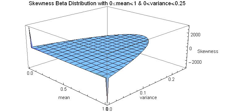
_(the_third_moment_centered_on_the_mean,_normalized_by_the_3/2_power_of_the_variance)_of_the_beta_distribution_is :\gamma_1_=\frac_=_\frac_. Letting_α_=_β_in_the_above_expression_one_obtains_γ1_=_0,_showing_once_again_that_for_α_=_β_the_distribution_is_symmetric_and_hence_the_skewness_is_zero._Positive_skew_(right-tailed)_for_α_<_β,_negative_skew_(left-tailed)_for_α_>_β. Using_the__parametrization_in_terms_of_mean_μ_and_sample_size_ν_=_α_+_β: :_\begin __\alpha_&__=_\mu_\nu_,\text\nu_=(\alpha_+_\beta)__>0\\ __\beta_&__=_(1_-_\mu)_\nu_,_\text\nu_=(\alpha_+_\beta)__>0. \end one_can_express_the_skewness_in_terms_of_the_mean_μ_and_the_sample_size_ν_as_follows: :\gamma_1_=\frac_=_\frac. The_skewness_can_also_be_expressed_just_in_terms_of_the_variance_''var''_and_the_mean_μ_as_follows: :\gamma_1_=\frac_=_\frac\text_\operatorname_<_\mu(1-\mu) The_accompanying_plot_of_skewness_as_a_function_of_variance_and_mean_shows_that_maximum_variance_(1/4)_is_coupled_with_zero_skewness_and_the_symmetry_condition_(μ_=_1/2),_and_that_maximum_skewness_(positive_or_negative_infinity)_occurs_when_the_mean_is_located_at_one_end_or_the_other,_so_that_the_"mass"_of_the_probability_distribution_is_concentrated_at_the_ends_(minimum_variance). The_following_expression_for_the_square_of_the_skewness,_in_terms_of_the_sample_size_ν_=_α_+_β_and_the_variance_''var'',_is_useful_for_the_method_of_moments_estimation_of_four_parameters: :(\gamma_1)^2_=\frac_=_\frac\bigg(\frac-4(1+\nu)\bigg) This_expression_correctly_gives_a_skewness_of_zero_for_α_=_β,_since_in_that_case_(see_):_\operatorname_=_\frac. For_the_symmetric_case_(α_=_β),_skewness_=_0_over_the_whole_range,_and_the_following_limits_apply: :\lim__\gamma_1_=_\lim__\gamma_1_=\lim__\gamma_1=\lim__\gamma_1=\lim__\gamma_1_=_0 For_the_asymmetric_cases_(α_≠_β)_the_following_limits_(with_only_the_noted_variable_approaching_the_limit)_can_be_obtained_from_the_above_expressions: :_\begin &\lim__\gamma_1_=\lim__\gamma_1_=_\infty\\ &\lim__\gamma_1__=_\lim__\gamma_1=_-_\infty\\ &\lim__\gamma_1_=_-\frac,\quad_\lim_(\lim__\gamma_1)_=_-\infty,\quad_\lim_(\lim__\gamma_1)_=_0\\ &\lim__\gamma_1_=_\frac,\quad_\lim_(\lim__\gamma_1)_=_\infty,\quad_\lim_(\lim__\gamma_1)_=_0\\ &\lim__\gamma_1_=_\frac,\quad_\lim_(\lim__\gamma_1)__=_\infty,\quad_\lim_(\lim__\gamma_1)_=_-_\infty \end


_Kurtosis

The_beta_distribution_has_been_applied_in_acoustic_analysis_to_assess_damage_to_gears,_as_the_kurtosis_of_the_beta_distribution_has_been_reported_to_be_a_good_indicator_of_the_condition_of_a_gear._Kurtosis_has_also_been_used_to_distinguish_the_seismic_signal_generated_by_a_person's_footsteps_from_other_signals._As_persons_or_other_targets_moving_on_the_ground_generate_continuous_signals_in_the_form_of_seismic_waves,_one_can_separate_different_targets_based_on_the_seismic_waves_they_generate._Kurtosis_is_sensitive_to_impulsive_signals,_so_it's_much_more_sensitive_to_the_signal_generated_by_human_footsteps_than_other_signals_generated_by_vehicles,_winds,_noise,_etc.__Unfortunately,_the_notation_for_kurtosis_has_not_been_standardized._Kenney_and_Keeping__use_the_symbol_γ2_for_the_excess_kurtosis_ In_probability_theory_and_statistics,_kurtosis_(from__el,_κυρτός,_''kyrtos''_or_''kurtos'',_meaning_"curved,_arching")_is_a_measure_of_the_"tailedness"_of_the_probability_distribution_of_a_real-valued_random_variable._Like_skewness,_kurtosi_...
,_but_Abramowitz_and_Stegun__use_different_terminology.__To_prevent_confusion__between_kurtosis_(the_fourth_moment_centered_on_the_mean,_normalized_by_the_square_of_the_variance)_and_excess_kurtosis,_when_using_symbols,_they_will_be_spelled_out_as_follows: :\begin \text _____&=\text_-_3\\ _____&=\frac-3\\ _____&=\frac\\ _____&=\frac _. \end Letting_α_=_β_in_the_above_expression_one_obtains :\text_=-_\frac_\text\alpha=\beta_. Therefore,_for_symmetric_beta_distributions,_the_excess_kurtosis_is_negative,_increasing_from_a_minimum_value_of_−2_at_the_limit_as__→_0,_and_approaching_a_maximum_value_of_zero_as__→_∞.__The_value_of_−2_is_the_minimum_value_of_excess_kurtosis_that_any_distribution_(not_just_beta_distributions,_but_any_distribution_of_any_possible_kind)_can_ever_achieve.__This_minimum_value_is_reached_when_all_the_probability_density_is_entirely_concentrated_at_each_end_''x''_=_0_and_''x''_=_1,_with_nothing_in_between:_a_2-point_Bernoulli_distribution_ In_probability_theory_and_statistics,_the_Bernoulli_distribution,_named_after_Swiss_mathematician__Jacob_Bernoulli,James_Victor_Uspensky:_''Introduction_to_Mathematical_Probability'',_McGraw-Hill,_New_York_1937,_page_45_is_the__discrete_probabi_...
_with_equal_probability_1/2_at_each_end_(a_coin_toss:_see_section_below_"Kurtosis_bounded_by_the_square_of_the_skewness"_for_further_discussion).__The_description_of_kurtosis_as_a_measure_of_the_"potential_outliers"_(or_"potential_rare,_extreme_values")_of_the_probability_distribution,_is_correct_for_all_distributions_including_the_beta_distribution._When_rare,_extreme_values_can_occur_in_the_beta_distribution,_the_higher_its_kurtosis;_otherwise,_the_kurtosis_is_lower._For_α_≠_β,_skewed_beta_distributions,_the_excess_kurtosis_can_reach_unlimited_positive_values_(particularly_for_α_→_0_for_finite_β,_or_for_β_→_0_for_finite_α)_because_the_side_away_from_the_mode_will_produce_occasional_extreme_values.__Minimum_kurtosis_takes_place_when_the_mass_density_is_concentrated_equally_at_each_end_(and_therefore_the_mean_is_at_the_center),_and_there_is_no_probability_mass_density_in_between_the_ends. Using_the__parametrization_in_terms_of_mean_μ_and_sample_size_ν_=_α_+_β: :_\begin __\alpha_&__=_\mu_\nu_,\text\nu_=(\alpha_+_\beta)__>0\\ __\beta_&__=_(1_-_\mu)_\nu_,_\text\nu_=(\alpha_+_\beta)__>0. \end one_can_express_the_excess_kurtosis_in_terms_of_the_mean_μ_and_the_sample_size_ν_as_follows: :\text_=\frac\bigg_(\frac_-_1_\bigg_) The_excess_kurtosis_can_also_be_expressed_in_terms_of_just_the_following_two_parameters:_the_variance_''var'',_and_the_sample_size_ν_as_follows: :\text_=\frac\left(\frac_-_6_-_5_\nu_\right)\text\text<_\mu(1-\mu) and,_in_terms_of_the_variance_''var''_and_the_mean_μ_as_follows: :\text_=\frac\text\text<_\mu(1-\mu) The_plot_of_excess_kurtosis_as_a_function_of_the_variance_and_the_mean_shows_that_the_minimum_value_of_the_excess_kurtosis_(−2,_which_is_the_minimum_possible_value_for_excess_kurtosis_for_any_distribution)_is_intimately_coupled_with_the_maximum_value_of_variance_(1/4)_and_the_symmetry_condition:_the_mean_occurring_at_the_midpoint_(μ_=_1/2)._This_occurs_for_the_symmetric_case_of_α_=_β_=_0,_with_zero_skewness.__At_the_limit,_this_is_the_2_point_Bernoulli_distribution_ In_probability_theory_and_statistics,_the_Bernoulli_distribution,_named_after_Swiss_mathematician__Jacob_Bernoulli,James_Victor_Uspensky:_''Introduction_to_Mathematical_Probability'',_McGraw-Hill,_New_York_1937,_page_45_is_the__discrete_probabi_...
_with_equal_probability_1/2_at_each__Dirac_delta_function_end_''x''_=_0_and_''x''_=_1_and_zero_probability_everywhere_else._(A_coin_toss:_one_face_of_the_coin_being_''x''_=_0_and_the_other_face_being_''x''_=_1.)__Variance_is_maximum_because_the_distribution_is_bimodal_with_nothing_in_between_the_two_modes_(spikes)_at_each_end.__Excess_kurtosis_is_minimum:_the_probability_density_"mass"_is_zero_at_the_mean_and_it_is_concentrated_at_the_two_peaks_at_each_end.__Excess_kurtosis_reaches_the_minimum_possible_value_(for_any_distribution)_when_the_probability_density_function_has_two_spikes_at_each_end:_it_is_bi-"peaky"_with_nothing_in_between_them. On_the_other_hand,_the_plot_shows_that_for_extreme_skewed_cases,_where_the_mean_is_located_near_one_or_the_other_end_(μ_=_0_or_μ_=_1),_the_variance_is_close_to_zero,_and_the_excess_kurtosis_rapidly_approaches_infinity_when_the_mean_of_the_distribution_approaches_either_end. Alternatively,_the_excess_kurtosis_can_also_be_expressed_in_terms_of_just_the_following_two_parameters:_the_square_of_the_skewness,_and_the_sample_size_ν_as_follows: :\text_=\frac\bigg(\frac_(\text)^2_-_1\bigg)\text^2-2<_\text<_\frac_(\text)^2 From_this_last_expression,_one_can_obtain_the_same_limits_published_practically_a_century_ago_by_Karl_Pearson_in_his_paper,_for_the_beta_distribution_(see_section_below_titled_"Kurtosis_bounded_by_the_square_of_the_skewness")._Setting_α_+_β=_ν_=__0_in_the_above_expression,_one_obtains_Pearson's_lower_boundary_(values_for_the_skewness_and_excess_kurtosis_below_the_boundary_(excess_kurtosis_+_2_−_skewness2_=_0)_cannot_occur_for_any_distribution,_and_hence_Karl_Pearson_appropriately_called_the_region_below_this_boundary_the_"impossible_region")._The_limit_of_α_+_β_=_ν_→_∞_determines_Pearson's_upper_boundary. :_\begin &\lim_\text__=_(\text)^2_-_2\\ &\lim_\text__=_\tfrac_(\text)^2 \end therefore: :(\text)^2-2<_\text<_\tfrac_(\text)^2 Values_of_ν_=_α_+_β_such_that_ν_ranges_from_zero_to_infinity,_0_<_ν_<_∞,_span_the_whole_region_of_the_beta_distribution_in_the_plane_of_excess_kurtosis_versus_squared_skewness. For_the_symmetric_case_(α_=_β),_the_following_limits_apply: :_\begin &\lim__\text_=__-_2_\\ &\lim__\text_=_0_\\ &\lim__\text_=_-_\frac \end For_the_unsymmetric_cases_(α_≠_β)_the_following_limits_(with_only_the_noted_variable_approaching_the_limit)_can_be_obtained_from_the_above_expressions: :_\begin &\lim_\text__=\lim__\text__=_\lim_\text__=_\lim_\text__=\infty\\ &\lim_\text__=_\frac,\text__\lim_(\lim__\text)__=_\infty,\text__\lim_(\lim__\text)__=_0\\ &\lim_\text__=_\frac,\text__\lim_(\lim__\text)__=_\infty,\text__\lim_(\lim__\text)__=_0\\ &\lim__\text__=_-_6_+_\frac,\text__\lim_(\lim__\text)__=_\infty,\text__\lim_(\lim__\text)__=_\infty \end


_Characteristic_function

The_Characteristic_function_(probability_theory), characteristic_function_is_the_Fourier_transform_of_the_probability_density_function.__The_characteristic_function_of_the_beta_distribution_is_confluent_hypergeometric_function, Kummer's_confluent_hypergeometric_function_(of_the_first_kind): :\begin \varphi_X(\alpha;\beta;t) &=_\operatorname\left[e^\right]\\ &=_\int_0^1_e^_f(x;\alpha,\beta)_dx_\\ &=_1F_1(\alpha;_\alpha+\beta;_it)\!\\ &=\sum_^\infty_\frac__\\ &=_1__+\sum_^_\left(_\prod_^_\frac_\right)_\frac \end where :_x^=x(x+1)(x+2)\cdots(x+n-1) is_the_rising_factorial,_also_called_the_"Pochhammer_symbol".__The_value_of_the_characteristic_function_for_''t''_=_0,_is_one: :_\varphi_X(\alpha;\beta;0)=_1F_1(\alpha;_\alpha+\beta;_0)_=_1__. Also,_the_real_and_imaginary_parts_of_the_characteristic_function_enjoy_the_following_symmetries_with_respect_to_the_origin_of_variable_''t'': :_\textrm_\left_[__1F_1(\alpha;_\alpha+\beta;_it)_\right_]_=_\textrm_\left_[__1F_1(\alpha;_\alpha+\beta;_-_it)_\right_]__ :_\textrm_\left_[__1F_1(\alpha;_\alpha+\beta;_it)_\right_]_=_-_\textrm_\left__[__1F_1(\alpha;_\alpha+\beta;_-_it)_\right_]__ The_symmetric_case_α_=_β_simplifies_the_characteristic_function_of_the_beta_distribution_to_a_Bessel_function,_since_in_the_special_case_α_+_β_=_2α_the_confluent_hypergeometric_function_(of_the_first_kind)_reduces_to_a_Bessel_function_(the_modified_Bessel_function_of_the_first_kind_I__)_using_Ernst_Kummer, Kummer's_second_transformation_as_follows: Another_example_of_the_symmetric_case_α_=_β_=_n/2_for_beamforming_applications_can_be_found_in_Figure_11_of_ :\begin__1F_1(\alpha;2\alpha;_it)_&=_e^__0F_1_\left(;_\alpha+\tfrac;_\frac_\right)_\\ &=_e^_\left(\frac\right)^_\Gamma\left(\alpha+\tfrac\right)_I_\left(\frac\right).\end In_the_accompanying_plots,_the_Complex_number, real_part_(Re)_of_the_Characteristic_function_(probability_theory), characteristic_function_of_the_beta_distribution_is_displayed_for_symmetric_(α_=_β)_and_skewed_(α_≠_β)_cases.


_Other_moments


_Moment_generating_function

It_also_follows_that_the_moment_generating_function_is :\begin M_X(\alpha;_\beta;_t) &=_\operatorname\left[e^\right]_\\_pt&=_\int_0^1_e^_f(x;\alpha,\beta)\,dx_\\_pt&=__1F_1(\alpha;_\alpha+\beta;_t)_\\_pt&=_\sum_^\infty_\frac__\frac_\\_pt&=_1__+\sum_^_\left(_\prod_^_\frac_\right)_\frac \end In_particular_''M''''X''(''α'';_''β'';_0)_=_1.


_Higher_moments

Using_the_moment_generating_function,_the_''k''-th_raw_moment_is_given_by_the_factor :\prod_^_\frac_ multiplying_the_(exponential_series)_term_\left(\frac\right)_in_the_series_of_the_moment_generating_function :\operatorname[X^k]=_\frac_=_\prod_^_\frac where_(''x'')(''k'')_is_a_Pochhammer_symbol_representing_rising_factorial._It_can_also_be_written_in_a_recursive_form_as :\operatorname[X^k]_=_\frac\operatorname[X^]. Since_the_moment_generating_function_M_X(\alpha;_\beta;_\cdot)_has_a_positive_radius_of_convergence,_the_beta_distribution_is_Moment_problem, determined_by_its_moments.


_Moments_of_transformed_random_variables


_=Moments_of_linearly_transformed,_product_and_inverted_random_variables

= One_can_also_show_the_following_expectations_for_a_transformed_random_variable,_where_the_random_variable_''X''_is_Beta-distributed_with_parameters_α_and_β:_''X''_~_Beta(α,_β).__The_expected_value_of_the_variable_1 − ''X''_is_the_mirror-symmetry_of_the_expected_value_based_on_''X'': :\begin &_\operatorname[1-X]_=_\frac_\\ &_\operatorname[X_(1-X)]_=\operatorname[(1-X)X_]_=\frac \end Due_to_the_mirror-symmetry_of_the_probability_density_function_of_the_beta_distribution,_the_variances_based_on_variables_''X''_and_1 − ''X''_are_identical,_and_the_covariance_on_''X''(1 − ''X''_is_the_negative_of_the_variance: :\operatorname[(1-X)]=\operatorname[X]_=_-\operatorname[X,(1-X)]=_\frac These_are_the_expected_values_for_inverted_variables,_(these_are_related_to_the_harmonic_means,_see_): :\begin &_\operatorname_\left_[\frac_\right_]_=_\frac_\text_\alpha_>_1\\ &_\operatorname\left_[\frac_\right_]_=\frac_\text_\beta_>_1 \end The_following_transformation_by_dividing_the_variable_''X''_by_its_mirror-image_''X''/(1 − ''X'')_results_in_the_expected_value_of_the_"inverted_beta_distribution"_or_beta_prime_distribution_ In_probability_theory_and__statistics,_the_beta_prime_distribution_(also_known_as_inverted_beta_distribution_or_beta_distribution_of_the_second_kindJohnson_et_al_(1995),_p_248)_is_an_absolutely_continuous_probability_distribution. __Definitions_ _...
_(also_known_as_beta_distribution_of_the_second_kind_or_Pearson_distribution, Pearson's_Type_VI): :_\begin &_\operatorname\left[\frac\right]_=\frac_\text\beta_>_1\\ &_\operatorname\left[\frac\right]_=\frac\text\alpha_>_1 \end_ Variances_of_these_transformed_variables_can_be_obtained_by_integration,_as_the_expected_values_of_the_second_moments_centered_on_the_corresponding_variables: :\operatorname_\left[\frac_\right]_=\operatorname\left[\left(\frac_-_\operatorname\left[\frac_\right_]_\right_)^2\right]= :\operatorname\left_[\frac_\right_]_=\operatorname_\left_[\left_(\frac_-_\operatorname\left_[\frac_\right_]_\right_)^2_\right_]=_\frac_\text\alpha_>_2 The_following_variance_of_the_variable_''X''_divided_by_its_mirror-image_(''X''/(1−''X'')_results_in_the_variance_of_the_"inverted_beta_distribution"_or_beta_prime_distribution_ In_probability_theory_and__statistics,_the_beta_prime_distribution_(also_known_as_inverted_beta_distribution_or_beta_distribution_of_the_second_kindJohnson_et_al_(1995),_p_248)_is_an_absolutely_continuous_probability_distribution. __Definitions_ _...
_(also_known_as_beta_distribution_of_the_second_kind_or_Pearson_distribution, Pearson's_Type_VI): :\operatorname_\left_[\frac_\right_]_=\operatorname_\left_[\left(\frac_-_\operatorname_\left_[\frac_\right_]_\right)^2_\right_]=\operatorname_\left_[\frac_\right_]_= :\operatorname_\left_[\left_(\frac_-_\operatorname_\left_[\frac_\right_]_\right_)^2_\right_]=_\frac_\text\beta_>_2 The_covariances_are: :\operatorname\left_[\frac,\frac_\right_]_=_\operatorname\left[\frac,\frac_\right]_=\operatorname\left[\frac,\frac\right_]_=_\operatorname\left[\frac,\frac_\right]_=\frac_\text_\alpha,_\beta_>_1 These_expectations_and_variances_appear_in_the_four-parameter_Fisher_information_matrix_(.)


_=Moments_of_logarithmically_transformed_random_variables

= Expected_values_for_Logarithm_transformation, logarithmic_transformations_(useful_for_maximum_likelihood_estimates,_see_)_are_discussed_in_this_section.__The_following_logarithmic_linear_transformations_are_related_to_the_geometric_means_''GX''_and__''G''(1−''X'')_(see_): :\begin \operatorname[\ln(X)]_&=_\psi(\alpha)_-_\psi(\alpha_+_\beta)=_-_\operatorname\left[\ln_\left_(\frac_\right_)\right],\\ \operatorname[\ln(1-X)]_&=\psi(\beta)_-_\psi(\alpha_+_\beta)=_-_\operatorname_\left[\ln_\left_(\frac_\right_)\right]. \end Where_the_digamma_function_ In_mathematics,_the_digamma_function_is_defined_as_the__logarithmic_derivative_of_the_gamma_function: :\psi(x)=\frac\ln\big(\Gamma(x)\big)=\frac\sim\ln-\frac. It_is_the_first_of_the__polygamma_functions._It_is_strictly_increasing_and_strict_...
_ψ(α)_is_defined_as_the_logarithmic_derivative_of_the_gamma_function_ In__mathematics,_the_gamma_function_(represented_by_,_the_capital_letter__gamma_from_the_Greek_alphabet)_is_one_commonly_used_extension_of_the__factorial_function_to_complex_numbers._The_gamma_function_is_defined_for_all_complex_numbers_except_...
: :\psi(\alpha)_=_\frac Logit_transformations_are_interesting,_as_they_usually_transform_various_shapes_(including_J-shapes)_into_(usually_skewed)_bell-shaped_densities_over_the_logit_variable,_and_they_may_remove_the_end_singularities_over_the_original_variable: :\begin \operatorname\left[\ln_\left_(\frac_\right_)_\right]_&=\psi(\alpha)_-_\psi(\beta)=_\operatorname[\ln(X)]_+\operatorname_\left[\ln_\left_(\frac_\right)_\right],\\ \operatorname\left_[\ln_\left_(\frac_\right_)_\right_]_&=\psi(\beta)_-_\psi(\alpha)=_-_\operatorname_\left[\ln_\left_(\frac_\right)_\right]_. \end Johnson__considered_the_distribution_of_the_logit_-_transformed_variable_ln(''X''/1−''X''),_including_its_moment_generating_function_and_approximations_for_large_values_of_the_shape_parameters.__This_transformation_extends_the_finite_support_,_1_ The_comma__is_a_punctuation_mark_that_appears_in_several_variants_in_different_languages._It_has_the_same_shape_as_an_apostrophe_or_single_closing_quotation_mark_()_in_many_typefaces,_but_it_differs_from_them_in_being_placed_on_the__baseline_o_...
based_on_the_original_variable_''X''_to_infinite_support_in_both_directions_of_the_real_line_(−∞,_+∞). Higher_order_logarithmic_moments_can_be_derived_by_using_the_representation_of_a_beta_distribution_as_a_proportion_of_two_Gamma_distributions_and_differentiating_through_the_integral._They_can_be_expressed_in_terms_of_higher_order_poly-gamma_functions_as_follows: :\begin \operatorname_\left_[\ln^2(X)_\right_]_&=_(\psi(\alpha)_-_\psi(\alpha_+_\beta))^2+\psi_1(\alpha)-\psi_1(\alpha+\beta),_\\ \operatorname_\left_[\ln^2(1-X)_\right_]_&=_(\psi(\beta)_-_\psi(\alpha_+_\beta))^2+\psi_1(\beta)-\psi_1(\alpha+\beta),_\\ \operatorname_\left_[\ln_(X)\ln(1-X)_\right_]_&=(\psi(\alpha)_-_\psi(\alpha_+_\beta))(\psi(\beta)_-_\psi(\alpha_+_\beta))_-\psi_1(\alpha+\beta). \end therefore_the_variance__ In_probability_theory_and_statistics,_variance_is_the__expectation_of_the_squared__deviation_of_a__random_variable_from_its__population_mean_or__sample_mean._Variance_is_a_measure_of_dispersion,_meaning_it_is_a_measure_of_how_far_a_set_of_numbe_...
_of_the_logarithmic_variables_and_covariance_ In__probability_theory_and__statistics,_covariance_is_a_measure_of_the_joint_variability_of_two__random_variables._If_the_greater_values_of_one_variable_mainly_correspond_with_the_greater_values_of_the_other_variable,_and_the_same_holds_for_the__...
_of_ln(''X'')_and_ln(1−''X'')_are: :\begin \operatorname[\ln(X),_\ln(1-X)]_&=_\operatorname\left[\ln(X)\ln(1-X)\right]_-_\operatorname[\ln(X)]\operatorname[\ln(1-X)]_=_-\psi_1(\alpha+\beta)_\\ &_\\ \operatorname[\ln_X]_&=_\operatorname[\ln^2(X)]_-_(\operatorname[\ln(X)])^2_\\ &=_\psi_1(\alpha)_-_\psi_1(\alpha_+_\beta)_\\ &=_\psi_1(\alpha)_+_\operatorname[\ln(X),_\ln(1-X)]_\\ &_\\ \operatorname_ln_(1-X)&=_\operatorname[\ln^2_(1-X)]_-_(\operatorname[\ln_(1-X)])^2_\\ &=_\psi_1(\beta)_-_\psi_1(\alpha_+_\beta)_\\ &=_\psi_1(\beta)_+_\operatorname[\ln_(X),_\ln(1-X)] \end where_the_trigamma_function_ In_mathematics,_the_trigamma_function,_denoted__or_,_is_the_second_of_the_polygamma_functions,_and_is_defined_by :_\psi_1(z)_=_\frac_\ln\Gamma(z). It_follows_from_this_definition_that :_\psi_1(z)_=_\frac_\psi(z) where__is_the_digamma_functio_...
,_denoted_ψ1(α),_is_the_second_of_the_polygamma_function_ In_mathematics,_the_polygamma_function_of_order__is_a_meromorphic_function_on_the__complex_numbers_\mathbb_defined_as_the_th__derivative_of_the_logarithm_of_the_gamma_function: :\psi^(z)_:=_\frac_\psi(z)_=_\frac_\ln\Gamma(z). Thus :\psi^(z)__...
s,_and_is_defined_as_the_derivative_of_the_digamma_function: :\psi_1(\alpha)_=_\frac=_\frac. The_variances_and_covariance_of_the_logarithmically_transformed_variables_''X''_and_(1−''X'')_are_different,_in_general,_because_the_logarithmic_transformation_destroys_the_mirror-symmetry_of_the_original_variables_''X''_and_(1−''X''),_as_the_logarithm_approaches_negative_infinity_for_the_variable_approaching_zero. These_logarithmic_variances_and_covariance_are_the_elements_of_the_Fisher_information_ In_mathematical_statistics,_the_Fisher_information_(sometimes_simply_called_information)_is_a_way_of_measuring_the_amount_of_information_that_an_observable_random_variable_''X''_carries_about_an_unknown_parameter_''θ''_of_a_distribution_that_model_...
_matrix_for_the_beta_distribution.__They_are_also_a_measure_of_the_curvature_of_the_log_likelihood_function_(see_section_on_Maximum_likelihood_estimation). The_variances_of_the_log_inverse_variables_are_identical_to_the_variances_of_the_log_variables: :\begin \operatorname\left[\ln_\left_(\frac_\right_)_\right]_&_=\operatorname[\ln(X)]_=_\psi_1(\alpha)_-_\psi_1(\alpha_+_\beta),_\\ \operatorname\left[\ln_\left_(\frac_\right_)_\right]_&=\operatorname_ln_(1-X)=_\psi_1(\beta)_-_\psi_1(\alpha_+_\beta),_\\ \operatorname\left[\ln_\left_(\frac_\right),_\ln_\left_(\frac\right_)_\right]_&=\operatorname[\ln(X),\ln(1-X)]=_-\psi_1(\alpha_+_\beta).\end It_also_follows_that_the_variances_of_the_logit_transformed_variables_are: :\operatorname\left[\ln_\left_(\frac_\right_)\right]=\operatorname\left[\ln_\left_(\frac_\right_)_\right]=-\operatorname\left_[\ln_\left_(\frac_\right_),_\ln_\left_(\frac_\right_)_\right]=_\psi_1(\alpha)_+_\psi_1(\beta)


_Quantities_of_information_(entropy)

Given_a_beta_distributed_random_variable,_''X''_~_Beta(''α'',_''β''),_the_information_entropy, differential_entropy_of_''X''_is_(measured_in_Nat_(unit), nats),_the_expected_value_of_the_negative_of_the_logarithm_of_the_probability_density_function_ In_probability_theory,_a_probability_density_function_(PDF),_or_density_of_a_continuous_random_variable,_is_a__function_whose_value_at_any_given_sample_(or_point)_in_the__sample_space_(the_set_of_possible_values_taken_by_the_random_variable)_ca_...
: :\begin h(X)_&=_\operatorname[-\ln(f(x;\alpha,\beta))]_\\_pt&=\int_0^1_-f(x;\alpha,\beta)\ln(f(x;\alpha,\beta))_\,_dx_\\_pt&=_\ln(\Beta(\alpha,\beta))-(\alpha-1)\psi(\alpha)-(\beta-1)\psi(\beta)+(\alpha+\beta-2)_\psi(\alpha+\beta) \end where_''f''(''x'';_''α'',_''β'')_is_the_probability_density_function_ In_probability_theory,_a_probability_density_function_(PDF),_or_density_of_a_continuous_random_variable,_is_a__function_whose_value_at_any_given_sample_(or_point)_in_the__sample_space_(the_set_of_possible_values_taken_by_the_random_variable)_ca_...
_of_the_beta_distribution: :f(x;\alpha,\beta)_=_\frac_x^(1-x)^ The_digamma_function_ In_mathematics,_the_digamma_function_is_defined_as_the__logarithmic_derivative_of_the_gamma_function: :\psi(x)=\frac\ln\big(\Gamma(x)\big)=\frac\sim\ln-\frac. It_is_the_first_of_the__polygamma_functions._It_is_strictly_increasing_and_strict_...
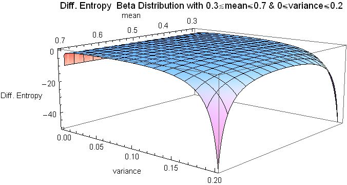
_''ψ''_appears_in_the_formula_for_the_differential_entropy_as_a_consequence_of_Euler's_integral_formula_for_the_harmonic_numbers_which_follows_from_the_integral: :\int_0^1_\frac__\,_dx_=_\psi(\alpha)-\psi(1) The_information_entropy, differential_entropy_of_the_beta_distribution_is_negative_for_all_values_of_''α''_and_''β''_greater_than_zero,_except_at_''α''_=_''β''_=_1_(for_which_values_the_beta_distribution_is_the_same_as_the_Uniform_distribution_(continuous), uniform_distribution),_where_the_information_entropy, differential_entropy_reaches_its_Maxima_and_minima, maximum_value_of_zero.__It_is_to_be_expected_that_the_maximum_entropy_should_take_place_when_the_beta_distribution_becomes_equal_to_the_uniform_distribution,_since_uncertainty_is_maximal_when_all_possible_events_are_equiprobable. For_''α''_or_''β''_approaching_zero,_the_information_entropy, differential_entropy_approaches_its_Maxima_and_minima, minimum_value_of_negative_infinity._For_(either_or_both)_''α''_or_''β''_approaching_zero,_there_is_a_maximum_amount_of_order:_all_the_probability_density_is_concentrated_at_the_ends,_and_there_is_zero_probability_density_at_points_located_between_the_ends._Similarly_for_(either_or_both)_''α''_or_''β''_approaching_infinity,_the_differential_entropy_approaches_its_minimum_value_of_negative_infinity,_and_a_maximum_amount_of_order.__If_either_''α''_or_''β''_approaches_infinity_(and_the_other_is_finite)_all_the_probability_density_is_concentrated_at_an_end,_and_the_probability_density_is_zero_everywhere_else.__If_both_shape_parameters_are_equal_(the_symmetric_case),_''α''_=_''β'',_and_they_approach_infinity_simultaneously,_the_probability_density_becomes_a_spike_(_Dirac_delta_function)_concentrated_at_the_middle_''x''_=_1/2,_and_hence_there_is_100%_probability_at_the_middle_''x''_=_1/2_and_zero_probability_everywhere_else. The_(continuous_case)_information_entropy, differential_entropy_was_introduced_by_Shannon_in_his_original_paper_(where_he_named_it_the_"entropy_of_a_continuous_distribution"),_as_the_concluding_part_of_the_same_paper_where_he_defined_the_information_entropy, discrete_entropy.__It_is_known_since_then_that_the_differential_entropy_may_differ_from_the_infinitesimal_limit_of_the_discrete_entropy_by_an_infinite_offset,_therefore_the_differential_entropy_can_be_negative_(as_it_is_for_the_beta_distribution)._What_really_matters_is_the_relative_value_of_entropy. Given_two_beta_distributed_random_variables,_''X''1_~_Beta(''α'',_''β'')_and_''X''2_~_Beta(''α''′,_''β''′),_the_cross_entropy_is_(measured_in_nats) :\begin H(X_1,X_2)_&=_\int_0^1_-_f(x;\alpha,\beta)_\ln_(f(x;\alpha',\beta'))_\,dx_\\_pt&=_\ln_\left(\Beta(\alpha',\beta')\right)-(\alpha'-1)\psi(\alpha)-(\beta'-1)\psi(\beta)+(\alpha'+\beta'-2)\psi(\alpha+\beta). \end The_cross_entropy_has_been_used_as_an_error_metric_to_measure_the_distance_between_two_hypotheses.__Its_absolute_value_is_minimum_when_the_two_distributions_are_identical._It_is_the_information_measure_most_closely_related_to_the_log_maximum_likelihood_(see_section_on_"Parameter_estimation._Maximum_likelihood_estimation")). The_relative_entropy,_or_Kullback–Leibler_divergence_''D''KL(''X''1_, , _''X''2),_is_a_measure_of_the_inefficiency_of_assuming_that_the_distribution_is_''X''2_~_Beta(''α''′,_''β''′)__when_the_distribution_is_really_''X''1_~_Beta(''α'',_''β'')._It_is_defined_as_follows_(measured_in_nats). :\begin D_(X_1, , X_2)_&=_\int_0^1_f(x;\alpha,\beta)_\ln_\left_(\frac_\right_)_\,_dx_\\_pt&=_\left_(\int_0^1_f(x;\alpha,\beta)_\ln_(f(x;\alpha,\beta))_\,dx_\right_)-_\left_(\int_0^1_f(x;\alpha,\beta)_\ln_(f(x;\alpha',\beta'))_\,_dx_\right_)\\_pt&=_-h(X_1)_+_H(X_1,X_2)\\_pt&=_\ln\left(\frac\right)+(\alpha-\alpha')\psi(\alpha)+(\beta-\beta')\psi(\beta)+(\alpha'-\alpha+\beta'-\beta)\psi_(\alpha_+_\beta). \end_ The_relative_entropy,_or_Kullback–Leibler_divergence,_is_always_non-negative.__A_few_numerical_examples_follow: *''X''1_~_Beta(1,_1)_and_''X''2_~_Beta(3,_3);_''D''KL(''X''1_, , _''X''2)_=_0.598803;_''D''KL(''X''2_, , _''X''1)_=_0.267864;_''h''(''X''1)_=_0;_''h''(''X''2)_=_−0.267864 *''X''1_~_Beta(3,_0.5)_and_''X''2_~_Beta(0.5,_3);_''D''KL(''X''1_, , _''X''2)_=_7.21574;_''D''KL(''X''2_, , _''X''1)_=_7.21574;_''h''(''X''1)_=_−1.10805;_''h''(''X''2)_=_−1.10805. The_Kullback–Leibler_divergence_is_not_symmetric_''D''KL(''X''1_, , _''X''2)_≠_''D''KL(''X''2_, , _''X''1)__for_the_case_in_which_the_individual_beta_distributions_Beta(1,_1)_and_Beta(3,_3)_are_symmetric,_but_have_different_entropies_''h''(''X''1)_≠_''h''(''X''2)._The_value_of_the_Kullback_divergence_depends_on_the_direction_traveled:_whether_going_from_a_higher_(differential)_entropy_to_a_lower_(differential)_entropy_or_the_other_way_around._In_the_numerical_example_above,_the_Kullback_divergence_measures_the_inefficiency_of_assuming_that_the_distribution_is_(bell-shaped)_Beta(3,_3),_rather_than_(uniform)_Beta(1,_1)._The_"h"_entropy_of_Beta(1,_1)_is_higher_than_the_"h"_entropy_of_Beta(3,_3)_because_the_uniform_distribution_Beta(1,_1)_has_a_maximum_amount_of_disorder._The_Kullback_divergence_is_more_than_two_times_higher_(0.598803_instead_of_0.267864)_when_measured_in_the_direction_of_decreasing_entropy:_the_direction_that_assumes_that_the_(uniform)_Beta(1,_1)_distribution_is_(bell-shaped)_Beta(3,_3)_rather_than_the_other_way_around._In_this_restricted_sense,_the_Kullback_divergence_is_consistent_with_the_second_law_of_thermodynamics. The_Kullback–Leibler_divergence_is_symmetric_''D''KL(''X''1_, , _''X''2)_=_''D''KL(''X''2_, , _''X''1)_for_the_skewed_cases_Beta(3,_0.5)_and_Beta(0.5,_3)_that_have_equal_differential_entropy_''h''(''X''1)_=_''h''(''X''2). The_symmetry_condition: :D_(X_1, , X_2)_=_D_(X_2, , X_1),\texth(X_1)_=_h(X_2),\text\alpha_\neq_\beta follows_from_the_above_definitions_and_the_mirror-symmetry_''f''(''x'';_''α'',_''β'')_=_''f''(1−''x'';_''α'',_''β'')_enjoyed_by_the_beta_distribution.


_Relationships_between_statistical_measures


_Mean,_mode_and_median_relationship

If_1_<_α_<_β_then_mode_≤_median_≤_mean.Kerman_J_(2011)_"A_closed-form_approximation_for_the_median_of_the_beta_distribution".__Expressing_the_mode_(only_for_α,_β_>_1),_and_the_mean_in_terms_of_α_and_β: :__\frac_\le_\text_\le_\frac_, If_1_<_β_<_α_then_the_order_of_the_inequalities_are_reversed._For_α,_β_>_1_the_absolute_distance_between_the_mean_and_the_median_is_less_than_5%_of_the_distance_between_the_maximum_and_minimum_values_of_''x''._On_the_other_hand,_the_absolute_distance_between_the_mean_and_the_mode_can_reach_50%_of_the_distance_between_the_maximum_and_minimum_values_of_''x'',_for_the_(Pathological_(mathematics), pathological)_case_of_α_=_1_and_β_=_1,_for_which_values_the_beta_distribution_approaches_the_uniform_distribution_and_the_information_entropy, differential_entropy_approaches_its_Maxima_and_minima, maximum_value,_and_hence_maximum_"disorder". For_example,_for_α_=_1.0001_and_β_=_1.00000001: *_mode___=_0.9999;___PDF(mode)_=_1.00010 *_mean___=_0.500025;_PDF(mean)_=_1.00003 *_median_=_0.500035;_PDF(median)_=_1.00003 *_mean_−_mode___=_−0.499875 *_mean_−_median_=_−9.65538_×_10−6 where_PDF_stands_for_the_value_of_the_probability_density_function_ In_probability_theory,_a_probability_density_function_(PDF),_or_density_of_a_continuous_random_variable,_is_a__function_whose_value_at_any_given_sample_(or_point)_in_the__sample_space_(the_set_of_possible_values_taken_by_the_random_variable)_ca_...
.


_Mean,_geometric_mean_and_harmonic_mean_relationship

It_is_known_from_the_inequality_of_arithmetic_and_geometric_means_that_the_geometric_mean_is_lower_than_the_mean.__Similarly,_the_harmonic_mean_is_lower_than_the_geometric_mean.__The_accompanying_plot_shows_that_for_α_=_β,_both_the_mean_and_the_median_are_exactly_equal_to_1/2,_regardless_of_the_value_of_α_=_β,_and_the_mode_is_also_equal_to_1/2_for_α_=_β_>_1,_however_the_geometric_and_harmonic_means_are_lower_than_1/2_and_they_only_approach_this_value_asymptotically_as_α_=_β_→_∞.


_Kurtosis_bounded_by_the_square_of_the_skewness

As_remarked_by_William_Feller, Feller,_in_the_Pearson_distribution, Pearson_system_the_beta_probability_density_appears_as_Pearson_distribution, type_I_(any_difference_between_the_beta_distribution_and_Pearson's_type_I_distribution_is_only_superficial_and_it_makes_no_difference_for_the_following_discussion_regarding_the_relationship_between_kurtosis_and_skewness)._Karl_Pearson_showed,_in_Plate_1_of_his_paper___published_in_1916,__a_graph_with_the_kurtosis_as_the_vertical_axis_(ordinate)_and_the_square_of_the_skewness_ In_probability_theory_and_statistics,_skewness_is_a_measure_of_the_asymmetry_of_the_probability_distribution_of_a__real-valued_random_variable_about_its_mean._The_skewness_value_can_be_positive,_zero,_negative,_or_undefined. For_a_unimodal__...
_as_the_horizontal_axis_(abscissa),_in_which_a_number_of_distributions_were_displayed.__The_region_occupied_by_the_beta_distribution_is_bounded_by_the_following_two_Line_(geometry), lines_in_the_(skewness2,kurtosis)_Cartesian_coordinate_system, plane,_or_the_(skewness2,excess_kurtosis)_Cartesian_coordinate_system, plane: :(\text)^2+1<_\text<_\frac_(\text)^2_+_3 or,_equivalently, :(\text)^2-2<_\text<_\frac_(\text)^2 At_a_time_when_there_were_no_powerful_digital_computers,_Karl_Pearson_accurately_computed_further_boundaries,_for_example,_separating_the_"U-shaped"_from_the_"J-shaped"_distributions._The_lower_boundary_line_(excess_kurtosis_+_2_−_skewness2_=_0)_is_produced_by_skewed_"U-shaped"_beta_distributions_with_both_values_of_shape_parameters_α_and_β_close_to_zero.__The_upper_boundary_line_(excess_kurtosis_−_(3/2)_skewness2_=_0)_is_produced_by_extremely_skewed_distributions_with_very_large_values_of_one_of_the_parameters_and_very_small_values_of_the_other_parameter.__Karl_Pearson_showed_that_this_upper_boundary_line_(excess_kurtosis_−_(3/2)_skewness2_=_0)_is_also_the_intersection_with_Pearson's_distribution_III,_which_has_unlimited_support_in_one_direction_(towards_positive_infinity),_and_can_be_bell-shaped_or_J-shaped._His_son,_Egon_Pearson,_showed_that_the_region_(in_the_kurtosis/squared-skewness_plane)_occupied_by_the_beta_distribution_(equivalently,_Pearson's_distribution_I)_as_it_approaches_this_boundary_(excess_kurtosis_−_(3/2)_skewness2_=_0)_is_shared_with_the_noncentral_chi-squared_distribution.__Karl_Pearson_(Pearson_1895,_pp. 357,_360,_373–376)_also_showed_that_the_gamma_distribution_is_a_Pearson_type_III_distribution._Hence_this_boundary_line_for_Pearson's_type_III_distribution_is_known_as_the_gamma_line._(This_can_be_shown_from_the_fact_that_the_excess_kurtosis_of_the_gamma_distribution_is_6/''k''_and_the_square_of_the_skewness_is_4/''k'',_hence_(excess_kurtosis_−_(3/2)_skewness2_=_0)_is_identically_satisfied_by_the_gamma_distribution_regardless_of_the_value_of_the_parameter_"k")._Pearson_later_noted_that_the_chi-squared_distribution_is_a_special_case_of_Pearson's_type_III_and_also_shares_this_boundary_line_(as_it_is_apparent_from_the_fact_that_for_the_chi-squared_distribution_the_excess_kurtosis_is_12/''k''_and_the_square_of_the_skewness_is_8/''k'',_hence_(excess_kurtosis_−_(3/2)_skewness2_=_0)_is_identically_satisfied_regardless_of_the_value_of_the_parameter_"k")._This_is_to_be_expected,_since_the_chi-squared_distribution_''X''_~_χ2(''k'')_is_a_special_case_of_the_gamma_distribution,_with_parametrization_X_~_Γ(k/2,_1/2)_where_k_is_a_positive_integer_that_specifies_the_"number_of_degrees_of_freedom"_of_the_chi-squared_distribution. An_example_of_a_beta_distribution_near_the_upper_boundary_(excess_kurtosis_−_(3/2)_skewness2_=_0)_is_given_by_α_=_0.1,_β_=_1000,_for_which_the_ratio_(excess_kurtosis)/(skewness2)_=_1.49835_approaches_the_upper_limit_of_1.5_from_below._An_example_of_a_beta_distribution_near_the_lower_boundary_(excess_kurtosis_+_2_−_skewness2_=_0)_is_given_by_α=_0.0001,_β_=_0.1,_for_which_values_the_expression_(excess_kurtosis_+_2)/(skewness2)_=_1.01621_approaches_the_lower_limit_of_1_from_above._In_the_infinitesimal_limit_for_both_α_and_β_approaching_zero_symmetrically,_the_excess_kurtosis_reaches_its_minimum_value_at_−2.__This_minimum_value_occurs_at_the_point_at_which_the_lower_boundary_line_intersects_the_vertical_axis_(ordinate)._(However,_in_Pearson's_original_chart,_the_ordinate_is_kurtosis,_instead_of_excess_kurtosis,_and_it_increases_downwards_rather_than_upwards). Values_for_the_skewness_and_excess_kurtosis_below_the_lower_boundary_(excess_kurtosis_+_2_−_skewness2_=_0)_cannot_occur_for_any_distribution,_and_hence_Karl_Pearson_appropriately_called_the_region_below_this_boundary_the_"impossible_region"._The_boundary_for_this_"impossible_region"_is_determined_by_(symmetric_or_skewed)_bimodal_"U"-shaped_distributions_for_which_the_parameters_α_and_β_approach_zero_and_hence_all_the_probability_density_is_concentrated_at_the_ends:_''x''_=_0,_1_with_practically_nothing_in_between_them._Since_for_α_≈_β_≈_0_the_probability_density_is_concentrated_at_the_two_ends_''x''_=_0_and_''x''_=_1,_this_"impossible_boundary"_is_determined_by_a_Bernoulli_distribution_ In_probability_theory_and_statistics,_the_Bernoulli_distribution,_named_after_Swiss_mathematician__Jacob_Bernoulli,James_Victor_Uspensky:_''Introduction_to_Mathematical_Probability'',_McGraw-Hill,_New_York_1937,_page_45_is_the__discrete_probabi_...
,_where_the_two_only_possible_outcomes_occur_with_respective_probabilities_''p''_and_''q''_=_1−''p''._For_cases_approaching_this_limit_boundary_with_symmetry_α_=_β,_skewness_≈_0,_excess_kurtosis_≈_−2_(this_is_the_lowest_excess_kurtosis_possible_for_any_distribution),_and_the_probabilities_are_''p''_≈_''q''_≈_1/2.__For_cases_approaching_this_limit_boundary_with_skewness,_excess_kurtosis_≈_−2_+_skewness2,_and_the_probability_density_is_concentrated_more_at_one_end_than_the_other_end_(with_practically_nothing_in_between),_with_probabilities_p_=_\tfrac_at_the_left_end_''x''_=_0_and_q_=_1-p_=_\tfrac_at_the_right_end_''x''_=_1.


_Symmetry

All_statements_are_conditional_on_α,_β_>_0 *_Probability_density_function_Symmetry, reflection_symmetry ::f(x;\alpha,\beta)_=_f(1-x;\beta,\alpha) *_Cumulative_distribution_function_Symmetry, reflection_symmetry_plus_unitary_Symmetry, translation ::F(x;\alpha,\beta)_=_I_x(\alpha,\beta)_=_1-_F(1-_x;\beta,\alpha)_=_1_-_I_(\beta,\alpha) *_Mode_Symmetry, reflection_symmetry_plus_unitary_Symmetry, translation ::\operatorname(\Beta(\alpha,_\beta))=_1-\operatorname(\Beta(\beta,_\alpha)),\text\Beta(\beta,_\alpha)\ne_\Beta(1,1) *_Median_Symmetry, reflection_symmetry_plus_unitary_Symmetry, translation ::\operatorname_(\Beta(\alpha,_\beta)_)=_1_-_\operatorname_(\Beta(\beta,_\alpha)) *_Mean_Symmetry, reflection_symmetry_plus_unitary_Symmetry, translation ::\mu_(\Beta(\alpha,_\beta)_)=_1_-_\mu_(\Beta(\beta,_\alpha)_) *_Geometric_Means_each_is_individually_asymmetric,_the_following_symmetry_applies_between_the_geometric_mean_based_on_''X''_and_the_geometric_mean_based_on_its_reflection_Reflection_or_reflexion_may_refer_to: _Science_and_technology *_Reflection_(physics),_a_common_wave_phenomenon **_Specular_reflection,_reflection_from_a_smooth_surface ***_Mirror_image,_a_reflection_in_a_mirror_or_in_water **__Signal_reflection,_in__...
_(1-X) ::G_X_(\Beta(\alpha,_\beta)_)=G_(\Beta(\beta,_\alpha)_)_ *_Harmonic_means_each_is_individually_asymmetric,_the_following_symmetry_applies_between_the_harmonic_mean_based_on_''X''_and_the_harmonic_mean_based_on_its_reflection_Reflection_or_reflexion_may_refer_to: _Science_and_technology *_Reflection_(physics),_a_common_wave_phenomenon **_Specular_reflection,_reflection_from_a_smooth_surface ***_Mirror_image,_a_reflection_in_a_mirror_or_in_water **__Signal_reflection,_in__...
_(1-X) ::H_X_(\Beta(\alpha,_\beta)_)=H_(\Beta(\beta,_\alpha)_)_\text_\alpha,_\beta_>_1__. *_Variance_symmetry ::\operatorname_(\Beta(\alpha,_\beta)_)=\operatorname_(\Beta(\beta,_\alpha)_) *_Geometric_variances_each_is_individually_asymmetric,_the_following_symmetry_applies_between_the_log_geometric_variance_based_on_X_and_the_log_geometric_variance_based_on_its_reflection_Reflection_or_reflexion_may_refer_to: _Science_and_technology *_Reflection_(physics),_a_common_wave_phenomenon **_Specular_reflection,_reflection_from_a_smooth_surface ***_Mirror_image,_a_reflection_in_a_mirror_or_in_water **__Signal_reflection,_in__...
_(1-X) ::\ln(\operatorname_(\Beta(\alpha,_\beta)))_=_\ln(\operatorname(\Beta(\beta,_\alpha)))_ *_Geometric_covariance_symmetry ::\ln_\operatorname(\Beta(\alpha,_\beta))=\ln_\operatorname(\Beta(\beta,_\alpha)) *_Mean_absolute_deviation_around_the_mean_symmetry ::\operatorname[, X_-_E _]_(\Beta(\alpha,_\beta))=\operatorname[, _X_-_E ]_(\Beta(\beta,_\alpha)) *_Skewness_Symmetry_(mathematics), skew-symmetry ::\operatorname_(\Beta(\alpha,_\beta)_)=_-_\operatorname_(\Beta(\beta,_\alpha)_) *_Excess_kurtosis_symmetry ::\text_(\Beta(\alpha,_\beta)_)=_\text_(\Beta(\beta,_\alpha)_) *_Characteristic_function_symmetry_of_Real_part_(with_respect_to_the_origin_of_variable_"t") ::_\text_[_1F_1(\alpha;_\alpha+\beta;_it)_]_=_\text_[__1F_1(\alpha;_\alpha+\beta;_-_it)]__ *_Characteristic_function_Symmetry_(mathematics), skew-symmetry_of_Imaginary_part_(with_respect_to_the_origin_of_variable_"t") ::_\text_[_1F_1(\alpha;_\alpha+\beta;_it)_]_=_-_\text_[__1F_1(\alpha;_\alpha+\beta;_-_it)_]__ *_Characteristic_function_symmetry_of_Absolute_value_(with_respect_to_the_origin_of_variable_"t") ::_\text_[__1F_1(\alpha;_\alpha+\beta;_it)_]_=_\text_[__1F_1(\alpha;_\alpha+\beta;_-_it)_]__ *_Differential_entropy_symmetry ::h(\Beta(\alpha,_\beta)_)=_h(\Beta(\beta,_\alpha)_) *_Relative_Entropy_(also_called_Kullback–Leibler_divergence)_symmetry ::D_(X_1, , X_2)_=_D_(X_2, , X_1),_\texth(X_1)_=_h(X_2)\text\alpha_\neq_\beta *_Fisher_information_matrix_symmetry ::__=__


_Geometry_of_the_probability_density_function


_Inflection_points

For_certain_values_of_the_shape_parameters_α_and_β,_the_probability_density_function_ In_probability_theory,_a_probability_density_function_(PDF),_or_density_of_a_continuous_random_variable,_is_a__function_whose_value_at_any_given_sample_(or_point)_in_the__sample_space_(the_set_of_possible_values_taken_by_the_random_variable)_ca_...
_has_inflection_points,_at_which_the_curvature_changes_sign.__The_position_of_these_inflection_points_can_be_useful_as_a_measure_of_the_Statistical_dispersion, dispersion_or_spread_of_the_distribution. Defining_the_following_quantity: :\kappa_=\frac Points_of_inflection_occur,_depending_on_the_value_of_the_shape_parameters_α_and_β,_as_follows: *(α_>_2,_β_>_2)_The_distribution_is_bell-shaped_(symmetric_for_α_=_β_and_skewed_otherwise),_with_two_inflection_points,_equidistant_from_the_mode: ::x_=_\text_\pm_\kappa_=_\frac *_(α_=_2,_β_>_2)_The_distribution_is_unimodal,_positively_skewed,_right-tailed,_with_one_inflection_point,_located_to_the_right_of_the_mode: ::x_=\text_+_\kappa_=_\frac *_(α_>_2,_β_=_2)_The_distribution_is_unimodal,_negatively_skewed,_left-tailed,_with_one_inflection_point,_located_to_the_left_of_the_mode: ::x_=_\text_-_\kappa_=_1_-_\frac *_(1_<_α_<_2,_β_>_2,_α+β>2)_The_distribution_is_unimodal,_positively_skewed,_right-tailed,_with_one_inflection_point,_located_to_the_right_of_the_mode: ::x_=\text_+_\kappa_=_\frac *(0_<_α_<_1,_1_<_β_<_2)_The_distribution_has_a_mode_at_the_left_end_''x''_=_0_and_it_is_positively_skewed,_right-tailed._There_is_one_inflection_point,_located_to_the_right_of_the_mode: ::x_=_\frac *(α_>_2,_1_<_β_<_2)_The_distribution_is_unimodal_negatively_skewed,_left-tailed,_with_one_inflection_point,_located_to_the_left_of_the_mode: ::x_=\text_-_\kappa_=_\frac *(1_<_α_<_2,__0_<_β_<_1)_The_distribution_has_a_mode_at_the_right_end_''x''=1_and_it_is_negatively_skewed,_left-tailed._There_is_one_inflection_point,_located_to_the_left_of_the_mode: ::x_=_\frac There_are_no_inflection_points_in_the_remaining_(symmetric_and_skewed)_regions:_U-shaped:_(α,_β_<_1)_upside-down-U-shaped:_(1_<_α_<_2,_1_<_β_<_2),_reverse-J-shaped_(α_<_1,_β_>_2)_or_J-shaped:_(α_>_2,_β_<_1) The_accompanying_plots_show_the_inflection_point_locations_(shown_vertically,_ranging_from_0_to_1)_versus_α_and_β_(the_horizontal_axes_ranging_from_0_to_5)._There_are_large_cuts_at_surfaces_intersecting_the_lines_α_=_1,_β_=_1,_α_=_2,_and_β_=_2_because_at_these_values_the_beta_distribution_change_from_2_modes,_to_1_mode_to_no_mode.


_Shapes

The_beta_density_function_can_take_a_wide_variety_of_different_shapes_depending_on_the_values_of_the_two_parameters_''α''_and_''β''.__The_ability_of_the_beta_distribution_to_take_this_great_diversity_of_shapes_(using_only_two_parameters)_is_partly_responsible_for_finding_wide_application_for_modeling_actual_measurements:


_=Symmetric_(''α''_=_''β'')

= *_the_density_function_is_symmetry, symmetric_about_1/2_(blue_&_teal_plots). *_median_=_mean_=_1/2. *skewness__=_0. *variance_=_1/(4(2α_+_1)) *α_=_β_<_1 **U-shaped_(blue_plot). **bimodal:_left_mode_=_0,__right_mode_=1,_anti-mode_=_1/2 **1/12_<_var(''X'')_<_1/4 **−2_<_excess_kurtosis(''X'')_<_−6/5 **_α_=_β_=_1/2_is_the__arcsine_distribution ***_var(''X'')_=_1/8 ***excess_kurtosis(''X'')_=_−3/2 ***CF_=_Rinc_(t)_ **_α_=_β_→_0_is_a_2-point_Bernoulli_distribution_ In_probability_theory_and_statistics,_the_Bernoulli_distribution,_named_after_Swiss_mathematician__Jacob_Bernoulli,James_Victor_Uspensky:_''Introduction_to_Mathematical_Probability'',_McGraw-Hill,_New_York_1937,_page_45_is_the__discrete_probabi_...
_with_equal_probability_1/2_at_each__Dirac_delta_function_end_''x''_=_0_and_''x''_=_1_and_zero_probability_everywhere_else._A_coin_toss:_one_face_of_the_coin_being_''x''_=_0_and_the_other_face_being_''x''_=_1. ***__\lim__\operatorname(X)_=_\tfrac_ ***__\lim__\operatorname(X)_=_-_2__a_lower_value_than_this_is_impossible_for_any_distribution_to_reach. ***_The_information_entropy, differential_entropy_approaches_a_Maxima_and_minima, minimum_value_of_−∞ *α_=_β_=_1 **the_uniform_distribution_(continuous), uniform_,_1_ The_comma__is_a_punctuation_mark_that_appears_in_several_variants_in_different_languages._It_has_the_same_shape_as_an_apostrophe_or_single_closing_quotation_mark_()_in_many_typefaces,_but_it_differs_from_them_in_being_placed_on_the__baseline_o_...
distribution **no_mode **var(''X'')_=_1/12 **excess_kurtosis(''X'')_=_−6/5 **The_(negative_anywhere_else)_information_entropy, differential_entropy_reaches_its_Maxima_and_minima, maximum_value_of_zero **CF_=_Sinc_(t) *''α''_=_''β''_>_1 **symmetric_unimodal **_mode_=_1/2. **0_<_var(''X'')_<_1/12 **−6/5_<_excess_kurtosis(''X'')_<_0 **''α''_=_''β''_=_3/2_is_a_semi-elliptic_,_1_ The_comma__is_a_punctuation_mark_that_appears_in_several_variants_in_different_languages._It_has_the_same_shape_as_an_apostrophe_or_single_closing_quotation_mark_()_in_many_typefaces,_but_it_differs_from_them_in_being_placed_on_the__baseline_o_...
distribution,_see:_Wigner_semicircle_distribution ***var(''X'')_=_1/16. ***excess_kurtosis(''X'')_=_−1 ***CF_=_2_Jinc_(t) **''α''_=_''β''_=_2_is_the_parabolic_,_1_ The_comma__is_a_punctuation_mark_that_appears_in_several_variants_in_different_languages._It_has_the_same_shape_as_an_apostrophe_or_single_closing_quotation_mark_()_in_many_typefaces,_but_it_differs_from_them_in_being_placed_on_the__baseline_o_...
distribution ***var(''X'')_=_1/20 ***excess_kurtosis(''X'')_=_−6/7 ***CF_=_3_Tinc_(t)_ **''α''_=_''β''_>_2_is_bell-shaped,_with_inflection_points_located_to_either_side_of_the_mode ***0_<_var(''X'')_<_1/20 ***−6/7_<_excess_kurtosis(''X'')_<_0 **''α''_=_''β''_→_∞_is_a_1-point_Degenerate_distribution_ In_mathematics,_a_degenerate_distribution_is,_according_to_some,_a_probability_distribution_in_a_space_with_support_only_on_a_manifold_of_lower_dimension,_and_according_to_others_a_distribution_with_support_only_at_a_single_point._By_the_latter_d_...
_with_a__Dirac_delta_function_spike_at_the_midpoint_''x''_=_1/2_with_probability_1,_and_zero_probability_everywhere_else._There_is_100%_probability_(absolute_certainty)_concentrated_at_the_single_point_''x''_=_1/2. ***_\lim__\operatorname(X)_=_0_ ***_\lim__\operatorname(X)_=_0 ***The_information_entropy, differential_entropy_approaches_a_Maxima_and_minima, minimum_value_of_−∞


_=Skewed_(''α''_≠_''β'')

= The_density_function_is_Skewness, skewed.__An_interchange_of_parameter_values_yields_the_mirror_image_(the_reverse)_of_the_initial_curve,_some_more_specific_cases: *''α''_<_1,_''β''_<_1 **_U-shaped **_Positive_skew_for_α_<_β,_negative_skew_for_α_>_β. **_bimodal:_left_mode_=_0,_right_mode_=_1,__anti-mode_=_\tfrac_ **_0_<_median_<_1. **_0_<_var(''X'')_<_1/4 *α_>_1,_β_>_1 **_unimodal_(magenta_&_cyan_plots), **Positive_skew_for_α_<_β,_negative_skew_for_α_>_β. **\text=_\tfrac_ **_0_<_median_<_1 **_0_<_var(''X'')_<_1/12 *α_<_1,_β_≥_1 **reverse_J-shaped_with_a_right_tail, **positively_skewed, **strictly_decreasing,_convex_function, convex **_mode_=_0 **_0_<_median_<_1/2. **_0_<_\operatorname(X)_<_\tfrac,__(maximum_variance_occurs_for_\alpha=\tfrac,_\beta=1,_or_α_=_Φ_the_Golden_ratio, golden_ratio_conjugate) *α_≥_1,_β_<_1 **J-shaped_with_a_left_tail, **negatively_skewed, **strictly_increasing,_convex_function, convex **_mode_=_1 **_1/2_<_median_<_1 **_0_<_\operatorname(X)_<_\tfrac,_(maximum_variance_occurs_for_\alpha=1,_\beta=\tfrac,_or_β_=_Φ_the_Golden_ratio, golden_ratio_conjugate) *α_=_1,_β_>_1 **positively_skewed, **strictly_decreasing_(red_plot), **a_reversed_(mirror-image)_power_function__,1distribution **_mean_=_1_/_(β_+_1) **_median_=_1_-_1/21/β **_mode_=_0 **α_=_1,_1_<_β_<_2 ***concave_function, concave ***_1-\tfrac<_\text_<_\tfrac ***_1/18_<_var(''X'')_<_1/12. **α_=_1,_β_=_2 ***a_straight_line_with_slope_−2,_the_right-triangular_distribution_with_right_angle_at_the_left_end,_at_''x''_=_0 ***_\text=1-\tfrac_ ***_var(''X'')_=_1/18 **α_=_1,_β_>_2 ***reverse_J-shaped_with_a_right_tail, ***convex_function, convex ***_0_<_\text_<_1-\tfrac ***_0_<_var(''X'')_<_1/18 *α_>_1,_β_=_1 **negatively_skewed, **strictly_increasing_(green_plot), **the_power_function_,_1_ The_comma__is_a_punctuation_mark_that_appears_in_several_variants_in_different_languages._It_has_the_same_shape_as_an_apostrophe_or_single_closing_quotation_mark_()_in_many_typefaces,_but_it_differs_from_them_in_being_placed_on_the__baseline_o_...
distribution **_mean_=_α_/_(α_+_1) **_median_=_1/21/α_ **_mode_=_1 **2_>_α_>_1,_β_=_1 ***concave_function, concave ***_\tfrac_<_\text_<_\tfrac ***_1/18_<_var(''X'')_<_1/12 **_α_=_2,_β_=_1 ***a_straight_line_with_slope_+2,_the_right-triangular_distribution_with_right_angle_at_the_right_end,_at_''x''_=_1 ***_\text=\tfrac_ ***_var(''X'')_=_1/18 **α_>_2,_β_=_1 ***J-shaped_with_a_left_tail,_convex_function, convex ***\tfrac_<_\text_<_1 ***_0_<_var(''X'')_<_1/18


_Related_distributions


_Transformations

*_If_''X''_~_Beta(''α'',_''β'')_then_1_−_''X''_~_Beta(''β'',_''α'')_Mirror_image, mirror-image_symmetry *_If_''X''_~_Beta(''α'',_''β'')_then_\tfrac_\sim_(\alpha,\beta)._The_beta_prime_distribution_ In_probability_theory_and__statistics,_the_beta_prime_distribution_(also_known_as_inverted_beta_distribution_or_beta_distribution_of_the_second_kindJohnson_et_al_(1995),_p_248)_is_an_absolutely_continuous_probability_distribution. __Definitions_ _...
,_also_called_"beta_distribution_of_the_second_kind". *_If_''X''_~_Beta(''α'',_''β'')_then_\tfrac_-1_\sim_(\beta,\alpha)._ *_If_''X''_~_Beta(''n''/2,_''m''/2)_then_\tfrac_\sim_F(n,m)_(assuming_''n''_>_0_and_''m''_>_0),_the_F-distribution, Fisher–Snedecor_F_distribution. *_If_X_\sim_\operatorname\left(1+\lambda\tfrac,_1_+_\lambda\tfrac\right)_then_min_+_''X''(max_−_min)_~_PERT(min,_max,_''m'',_''λ'')_where_''PERT''_denotes_a_PERT_distribution_used_in_PERT_analysis,_and_''m''=most_likely_value.Herrerías-Velasco,_José_Manuel_and_Herrerías-Pleguezuelo,_Rafael_and_René_van_Dorp,_Johan._(2011)._Revisiting_the_PERT_mean_and_Variance._European_Journal_of_Operational_Research_(210),_p._448–451._Traditionally_''λ''_=_4_in_PERT_analysis. *_If_''X''_~_Beta(1,_''β'')_then_''X''_~_Kumaraswamy_distribution_with_parameters_(1,_''β'') *_If_''X''_~_Beta(''α'',_1)_then_''X''_~_Kumaraswamy_distribution_with_parameters_(''α'',_1) *_If_''X''_~_Beta(''α'',_1)_then_−ln(''X'')_~_Exponential(''α'')


_Special_and_limiting_cases

*_Beta(1,_1)_~_uniform_distribution_(continuous), U(0,_1). *_Beta(n,_1)_~_Maximum_of_''n''_independent_rvs._with_uniform_distribution_(continuous), U(0,_1),_sometimes_called_a_''a_standard_power_function_distribution''_with_density_''n'' ''x''''n''-1_on_that_interval. *_Beta(1,_n)_~_Minimum_of_''n''_independent_rvs._with_uniform_distribution_(continuous), U(0,_1) *_If_''X''_~_Beta(3/2,_3/2)_and_''r''_>_0_then_2''rX'' − ''r''_~_Wigner_semicircle_distribution. *_Beta(1/2,_1/2)_is_equivalent_to_the__arcsine_distribution._This_distribution_is_also_Jeffreys_prior_probability_for_the_Bernoulli_Bernoulli_can_refer_to: _People *Bernoulli_family_of_17th_and_18th_century_Swiss_mathematicians: **_Daniel_Bernoulli_(1700–1782),_developer_of_Bernoulli's_principle **Jacob_Bernoulli_(1654–1705),_also_known_as_Jacques,_after_whom_Bernoulli_numbe_...
_and__binomial_distributions._The_arcsine_probability_density_is_a_distribution_that_appears_in_several_random-walk_fundamental_theorems._In_a_fair_coin_toss_random_walk_ In__mathematics,_a_random_walk_is_a_random_process_that_describes_a_path_that_consists_of_a_succession_of_random_steps_on_some_mathematical_space. An_elementary_example_of_a_random_walk_is_the_random_walk_on_the_integer_number_line_\mathbb_Z_...
,_the_probability_for_the_time_of_the_last_visit_to_the_origin_is_distributed_as_an_(U-shaped)__arcsine_distribution.__In_a_two-player_fair-coin-toss_game,_a_player_is_said_to_be_in_the_lead_if_the_random_walk_(that_started_at_the_origin)_is_above_the_origin.__The_most_probable_number_of_times_that_a_given_player_will_be_in_the_lead,_in_a_game_of_length_2''N'',_is_not_''N''.__On_the_contrary,_''N''_is_the_least_likely_number_of_times_that_the_player_will_be_in_the_lead._The_most_likely_number_of_times_in_the_lead_is_0_or_2''N''_(following_the__arcsine_distribution). *_\lim__n_\operatorname(1,n)_=__\operatorname(1)__the_exponential_distribution. *_\lim__n_\operatorname(k,n)_=_\operatorname(k,1)_the_gamma_distribution. *_For_large_n,_\operatorname(\alpha_n,\beta_n)_\to_\mathcal\left(\frac,\frac\frac\right)_the_normal_distribution._More_precisely,_if_X_n_\sim_\operatorname(\alpha_n,\beta_n)_then__\sqrt\left(X_n_-\tfrac\right)_converges_in_distribution_to_a_normal_distribution_with_mean_0_and_variance_\tfrac_as_''n''_increases.


_Derived_from_other_distributions

*_The_''k''th_order_statistic_of_a_sample_of_size_''n''_from_the_Uniform_distribution_(continuous), uniform_distribution_is_a_beta_random_variable,_''U''(''k'')_~_Beta(''k'',_''n''+1−''k''). *_If_''X''_~_Gamma(α,_θ)_and_''Y''_~_Gamma(β,_θ)_are_independent,_then_\tfrac_\sim_\operatorname(\alpha,_\beta)\,. *_If_X_\sim_\chi^2(\alpha)\,_and_Y_\sim_\chi^2(\beta)\,_are_independent,_then_\tfrac_\sim_\operatorname(\tfrac,_\tfrac). *_If_''X''_~_U(0,_1)_and_''α''_>_0_then_''X''1/''α''_~_Beta(''α'',_1)._The_power_function_distribution. *_If__X_\sim\operatorname(k;n;p),_then_\sim_\operatorname(\alpha,_\beta)_for_discrete_values_of_''n''_and_''k''_where_\alpha=k+1_and_\beta=n-k+1. *_If_''X''_~_Cauchy(0,_1)_then_\tfrac_\sim_\operatorname\left(\tfrac12,_\tfrac12\right)\,


_Combination_with_other_distributions

*_''X''_~_Beta(''α'',_''β'')_and_''Y''_~_F(2''β'',2''α'')_then__\Pr(X_\leq_\tfrac_\alpha_)_=_\Pr(Y_\geq_x)\,_for_all_''x''_>_0.


_Compounding_with_other_distributions

*_If_''p''_~_Beta(α,_β)_and_''X''_~_Bin(''k'',_''p'')_then_''X''_~_beta-binomial_distribution *_If_''p''_~_Beta(α,_β)_and_''X''_~_NB(''r'',_''p'')_then_''X''_~_beta_negative_binomial_distribution


_Generalisations

*_The_generalization_to_multiple_variables,_i.e._a_Dirichlet_distribution, multivariate_Beta_distribution,_is_called_a_Dirichlet_distribution_ In_probability_and__statistics,_the_Dirichlet_distribution_(after_Peter_Gustav_Lejeune_Dirichlet),_often_denoted_\operatorname(\boldsymbol\alpha),_is_a_family_of__continuous__multivariate__probability_distributions_parameterized_by_a_vector_\bold_...
._Univariate_marginals_of_the_Dirichlet_distribution_have_a_beta_distribution.__The_beta_distribution_is_Conjugate_prior, conjugate_to_the_binomial_and_Bernoulli_distributions_in_exactly_the_same_way_as_the_Dirichlet_distribution_ In_probability_and__statistics,_the_Dirichlet_distribution_(after_Peter_Gustav_Lejeune_Dirichlet),_often_denoted_\operatorname(\boldsymbol\alpha),_is_a_family_of__continuous__multivariate__probability_distributions_parameterized_by_a_vector_\bold_...
_is_conjugate_to_the_multinomial_distribution_and_categorical_distribution. *_The_Pearson_distribution#The_Pearson_type_I_distribution, Pearson_type_I_distribution_is_identical_to_the_beta_distribution_(except_for_arbitrary_shifting_and_re-scaling_that_can_also_be_accomplished_with_the_four_parameter_parametrization_of_the_beta_distribution). *_The_beta_distribution_is_the_special_case_of_the_noncentral_beta_distribution_where_\lambda_=_0:_\operatorname(\alpha,_\beta)_=_\operatorname(\alpha,\beta,0). *_The_generalized_beta_distribution_is_a_five-parameter_distribution_family_which_has_the_beta_distribution_as_a_special_case. *_The_matrix_variate_beta_distribution_is_a_distribution_for_positive-definite_matrices.


__Statistical_inference_


_Parameter_estimation


_Method_of_moments


_=Two_unknown_parameters

= Two_unknown_parameters_(_(\hat,_\hat)__of_a_beta_distribution_supported_in_the__,1interval)_can_be_estimated,_using_the_method_of_moments,_with_the_first_two_moments_(sample_mean_and_sample_variance)_as_follows.__Let: :_\text=\bar_=_\frac\sum_^N_X_i be_the_sample_mean_estimate_and :_\text_=\bar_=_\frac\sum_^N_(X_i_-_\bar)^2 be_the_sample_variance_estimate.__The_method_of_moments_(statistics), method-of-moments_estimates_of_the_parameters_are :\hat_=_\bar_\left(\frac_-_1_\right),_if_\bar_<\bar(1_-_\bar), :_\hat_=_(1-\bar)_\left(\frac_-_1_\right),_if_\bar<\bar(1_-_\bar). When_the_distribution_is_required_over_a_known_interval_other_than_,_1_ The_comma__is_a_punctuation_mark_that_appears_in_several_variants_in_different_languages._It_has_the_same_shape_as_an_apostrophe_or_single_closing_quotation_mark_()_in_many_typefaces,_but_it_differs_from_them_in_being_placed_on_the__baseline_o_...
with_random_variable_''X'',_say_[''a'',_''c'']_with_random_variable_''Y'',_then_replace_\bar_with_\frac,_and_\bar_with_\frac_in_the_above_couple_of_equations_for_the_shape_parameters_(see_the_"Alternative_parametrizations,_four_parameters"_section_below).,_where: :_\text=\bar_=_\frac\sum_^N_Y_i :_\text_=_\bar_=_\frac\sum_^N_(Y_i_-_\bar)^2


_=Four_unknown_parameters

= All_four_parameters_(\hat,_\hat,_\hat,_\hat_of_a_beta_distribution_supported_in_the_[''a'',_''c'']_interval_-see_section_Beta_distribution#Four_parameters_2, "Alternative_parametrizations,_Four_parameters"-)_can_be_estimated,_using_the_method_of_moments_developed_by_Karl_Pearson,_by_equating_sample_and_population_values_of_the_first_four_central_moments_(mean,_variance,_skewness_and_excess_kurtosis)._The_excess_kurtosis_was_expressed_in_terms_of_the_square_of_the_skewness,_and_the_sample_size_ν_=_α_+_β,_(see_previous_section_Beta_distribution#Kurtosis, "Kurtosis")_as_follows: :\text_=\frac\left(\frac_(\text)^2_-_1\right)\text^2-2<_\text<_\tfrac_(\text)^2 One_can_use_this_equation_to_solve_for_the_sample_size_ν=_α_+_β_in_terms_of_the_square_of_the_skewness_and_the_excess_kurtosis_as_follows: :\hat_=_\hat_+_\hat_=_3\frac :\text^2-2<_\text<_\tfrac_(\text)^2 This_is_the_ratio_(multiplied_by_a_factor_of_3)_between_the_previously_derived_limit_boundaries_for_the_beta_distribution_in_a_space_(as_originally_done_by_Karl_Pearson)_defined_with_coordinates_of_the_square_of_the_skewness_in_one_axis_and_the_excess_kurtosis_in_the_other_axis_(see_): The_case_of_zero_skewness,_can_be_immediately_solved_because_for_zero_skewness,_α_=_β_and_hence_ν_=_2α_=_2β,_therefore_α_=_β_=_ν/2 :_\hat_=_\hat_=_\frac=_\frac :__\text=_0_\text_-2<\text<0 (Excess_kurtosis_is_negative_for_the_beta_distribution_with_zero_skewness,_ranging_from_-2_to_0,_so_that_\hat_-and_therefore_the_sample_shape_parameters-_is_positive,_ranging_from_zero_when_the_shape_parameters_approach_zero_and_the_excess_kurtosis_approaches_-2,_to_infinity_when_the_shape_parameters_approach_infinity_and_the_excess_kurtosis_approaches_zero). For_non-zero_sample_skewness_one_needs_to_solve_a_system_of_two_coupled_equations._Since_the_skewness_and_the_excess_kurtosis_are_independent_of_the_parameters_\hat,_\hat,_the_parameters_\hat,_\hat_can_be_uniquely_determined_from_the_sample_skewness_and_the_sample_excess_kurtosis,_by_solving_the_coupled_equations_with_two_known_variables_(sample_skewness_and_sample_excess_kurtosis)_and_two_unknowns_(the_shape_parameters): :(\text)^2_=_\frac :\text_=\frac\left(\frac_(\text)^2_-_1\right) :\text^2-2<_\text<_\tfrac(\text)^2 resulting_in_the_following_solution: :_\hat,_\hat_=_\frac_\left_(1_\pm_\frac_\right_) :_\text\neq_0_\text_(\text)^2-2<_\text<_\tfrac_(\text)^2 Where_one_should_take_the_solutions_as_follows:_\hat>\hat_for_(negative)_sample_skewness_<_0,_and_\hat<\hat_for_(positive)_sample_skewness_>_0. The_accompanying_plot_shows_these_two_solutions_as_surfaces_in_a_space_with_horizontal_axes_of_(sample_excess_kurtosis)_and_(sample_squared_skewness)_and_the_shape_parameters_as_the_vertical_axis._The_surfaces_are_constrained_by_the_condition_that_the_sample_excess_kurtosis_must_be_bounded_by_the_sample_squared_skewness_as_stipulated_in_the_above_equation.__The_two_surfaces_meet_at_the_right_edge_defined_by_zero_skewness._Along_this_right_edge,_both_parameters_are_equal_and_the_distribution_is_symmetric_U-shaped_for_α_=_β_<_1,_uniform_for_α_=_β_=_1,_upside-down-U-shaped_for_1_<_α_=_β_<_2_and_bell-shaped_for_α_=_β_>_2.__The_surfaces_also_meet_at_the_front_(lower)_edge_defined_by_"the_impossible_boundary"_line_(excess_kurtosis_+_2_-_skewness2_=_0)._Along_this_front_(lower)_boundary_both_shape_parameters_approach_zero,_and_the_probability_density_is_concentrated_more_at_one_end_than_the_other_end_(with_practically_nothing_in_between),_with_probabilities_p=\tfrac_at_the_left_end_''x''_=_0_and_q_=_1-p_=_\tfrac___at_the_right_end_''x''_=_1.__The_two_surfaces_become_further_apart_towards_the_rear_edge.__At_this_rear_edge_the_surface_parameters_are_quite_different_from_each_other.__As_remarked,_for_example,_by_Bowman_and_Shenton,_sampling_in_the_neighborhood_of_the_line_(sample_excess_kurtosis_-_(3/2)(sample_skewness)2_=_0)_(the_just-J-shaped_portion_of_the_rear_edge_where_blue_meets_beige),_"is_dangerously_near_to_chaos",_because_at_that_line_the_denominator_of_the_expression_above_for_the_estimate_ν_=_α_+_β_becomes_zero_and_hence_ν_approaches_infinity_as_that_line_is_approached.__Bowman_and_Shenton__write_that_"the_higher_moment_parameters_(kurtosis_and_skewness)_are_extremely_fragile_(near_that_line)._However,_the_mean_and_standard_deviation_are_fairly_reliable."_Therefore,_the_problem_is_for_the_case_of_four_parameter_estimation_for_very_skewed_distributions_such_that_the_excess_kurtosis_approaches_(3/2)_times_the_square_of_the_skewness.__This_boundary_line_is_produced_by_extremely_skewed_distributions_with_very_large_values_of_one_of_the_parameters_and_very_small_values_of_the_other_parameter.__See__for_a_numerical_example_and_further_comments_about_this_rear_edge_boundary_line_(sample_excess_kurtosis_-_(3/2)(sample_skewness)2_=_0).__As_remarked_by_Karl_Pearson_himself__this_issue_may_not_be_of_much_practical_importance_as_this_trouble_arises_only_for_very_skewed_J-shaped_(or_mirror-image_J-shaped)_distributions_with_very_different_values_of_shape_parameters_that_are_unlikely_to_occur_much_in_practice).__The_usual_skewed-bell-shape_distributions_that_occur_in_practice_do_not_have_this_parameter_estimation_problem. The_remaining_two_parameters_\hat,_\hat_can_be_determined_using_the_sample_mean_and_the_sample_variance_using_a_variety_of_equations.__One_alternative_is_to_calculate_the_support_interval_range_(\hat-\hat)_based_on_the_sample_variance_and_the_sample_kurtosis.__For_this_purpose_one_can_solve,_in_terms_of_the_range_(\hat-_\hat),_the_equation_expressing_the_excess_kurtosis_in_terms_of_the_sample_variance,_and_the_sample_size_ν_(see__and_): :\text_=\frac\bigg(\frac_-_6_-_5_\hat_\bigg) to_obtain: :_(\hat-_\hat)_=_\sqrt\sqrt Another_alternative_is_to_calculate_the_support_interval_range_(\hat-\hat)_based_on_the_sample_variance_and_the_sample_skewness.__For_this_purpose_one_can_solve,_in_terms_of_the_range_(\hat-\hat),_the_equation_expressing_the_squared_skewness_in_terms_of_the_sample_variance,_and_the_sample_size_ν_(see_section_titled_"Skewness"_and_"Alternative_parametrizations,_four_parameters"): :(\text)^2_=_\frac\bigg(\frac-4(1+\hat)\bigg) to_obtain: :_(\hat-_\hat)_=_\frac\sqrt The_remaining_parameter_can_be_determined_from_the_sample_mean_and_the_previously_obtained_parameters:_(\hat-\hat),_\hat,_\hat_=_\hat+\hat: :__\hat_=_(\text)_-__\left(\frac\right)(\hat-\hat)_ and_finally,_\hat=_(\hat-_\hat)_+_\hat__. In_the_above_formulas_one_may_take,_for_example,_as_estimates_of_the_sample_moments: :\begin \text_&=\overline_=_\frac\sum_^N_Y_i_\\ \text_&=_\overline_Y_=_\frac\sum_^N_(Y_i_-_\overline)^2_\\ \text_&=_G_1_=_\frac_\frac_\\ \text_&=_G_2_=_\frac_\frac_-_\frac \end The_estimators_''G''1_for_skewness, sample_skewness_and_''G''2_for_kurtosis, sample_kurtosis_are_used_by_DAP_(software), DAP/SAS_System, SAS,_PSPP/SPSS,_and_Microsoft_Excel, Excel.__However,_they_are_not_used_by_BMDP_and_(according_to_)_they_were_not_used_by_MINITAB_in_1998._Actually,_Joanes_and_Gill_in_their_1998_study__concluded_that_the_skewness_and_kurtosis_estimators_used_in_BMDP_and_in_MINITAB_(at_that_time)_had_smaller_variance_and_mean-squared_error_in_normal_samples,_but_the_skewness_and_kurtosis_estimators_used_in__DAP_(software), DAP/SAS_System, SAS,_PSPP/SPSS,_namely_''G''1_and_''G''2,_had_smaller_mean-squared_error_in_samples_from_a_very_skewed_distribution.__It_is_for_this_reason_that_we_have_spelled_out_"sample_skewness",_etc.,_in_the_above_formulas,_to_make_it_explicit_that_the_user_should_choose_the_best_estimator_according_to_the_problem_at_hand,_as_the_best_estimator_for_skewness_and_kurtosis_depends_on_the_amount_of_skewness_(as_shown_by_Joanes_and_Gill).


_Maximum_likelihood


_=Two_unknown_parameters

= As_is_also_the_case_for_maximum_likelihood_estimates_for_the_gamma_distribution,_the_maximum_likelihood_estimates_for_the_beta_distribution_do_not_have_a_general_closed_form_solution_for_arbitrary_values_of_the_shape_parameters._If_''X''1,_...,_''XN''_are_independent_random_variables_each_having_a_beta_distribution,_the_joint_log_likelihood_function_for_''N''_independent_and_identically_distributed_random_variables, iid_observations_is: :\begin \ln\,_\mathcal_(\alpha,_\beta\mid_X)_&=_\sum_^N_\ln_\left_(\mathcal_i_(\alpha,_\beta\mid_X_i)_\right_)\\ &=_\sum_^N_\ln_\left_(f(X_i;\alpha,\beta)_\right_)_\\ &=_\sum_^N_\ln_\left_(\frac_\right_)_\\ &=_(\alpha_-_1)\sum_^N_\ln_(X_i)_+_(\beta-_1)\sum_^N__\ln_(1-X_i)_-_N_\ln_\Beta(\alpha,\beta) \end Finding_the_maximum_with_respect_to_a_shape_parameter_involves_taking_the_partial_derivative_with_respect_to_the_shape_parameter_and_setting_the_expression_equal_to_zero_yielding_the_maximum_likelihood_estimator_of_the_shape_parameters: :\frac_=_\sum_^N_\ln_X_i_-N\frac=0 :\frac_=_\sum_^N__\ln_(1-X_i)-_N\frac=0 where: :\frac_=_-\frac+_\frac+_\frac=-\psi(\alpha_+_\beta)_+_\psi(\alpha)_+_0 :\frac=_-_\frac+_\frac_+_\frac=-\psi(\alpha_+_\beta)_+_0_+_\psi(\beta) since_the_digamma_function_ In_mathematics,_the_digamma_function_is_defined_as_the__logarithmic_derivative_of_the_gamma_function: :\psi(x)=\frac\ln\big(\Gamma(x)\big)=\frac\sim\ln-\frac. It_is_the_first_of_the__polygamma_functions._It_is_strictly_increasing_and_strict_...
_denoted_ψ(α)_is_defined_as_the_logarithmic_derivative_of_the_gamma_function_ In__mathematics,_the_gamma_function_(represented_by_,_the_capital_letter__gamma_from_the_Greek_alphabet)_is_one_commonly_used_extension_of_the__factorial_function_to_complex_numbers._The_gamma_function_is_defined_for_all_complex_numbers_except_...
: :\psi(\alpha)_=\frac_ To_ensure_that_the_values_with_zero_tangent_slope_are_indeed_a_maximum_(instead_of_a_saddle-point_or_a_minimum)_one_has_to_also_satisfy_the_condition_that_the_curvature_is_negative.__This_amounts_to_satisfying_that_the_second_partial_derivative_with_respect_to_the_shape_parameters_is_negative :\frac=_-N\frac<0 :\frac_=_-N\frac<0 using_the_previous_equations,_this_is_equivalent_to: :\frac_=_\psi_1(\alpha)-\psi_1(\alpha_+_\beta)_>_0 :\frac_=_\psi_1(\beta)_-\psi_1(\alpha_+_\beta)_>_0 where_the_trigamma_function_ In_mathematics,_the_trigamma_function,_denoted__or_,_is_the_second_of_the_polygamma_functions,_and_is_defined_by :_\psi_1(z)_=_\frac_\ln\Gamma(z). It_follows_from_this_definition_that :_\psi_1(z)_=_\frac_\psi(z) where__is_the_digamma_functio_...
,_denoted_''ψ''1(''α''),_is_the_second_of_the_polygamma_function_ In_mathematics,_the_polygamma_function_of_order__is_a_meromorphic_function_on_the__complex_numbers_\mathbb_defined_as_the_th__derivative_of_the_logarithm_of_the_gamma_function: :\psi^(z)_:=_\frac_\psi(z)_=_\frac_\ln\Gamma(z). Thus :\psi^(z)__...
s,_and_is_defined_as_the_derivative_of_the_digamma_function: :\psi_1(\alpha)_=_\frac=\,_\frac. These_conditions_are_equivalent_to_stating_that_the_variances_of_the_logarithmically_transformed_variables_are_positive,_since: :\operatorname[\ln_(X)]_=_\operatorname[\ln^2_(X)]_-_(\operatorname[\ln_(X)])^2_=_\psi_1(\alpha)_-_\psi_1(\alpha_+_\beta)_ :\operatorname_ln_(1-X)=_\operatorname[\ln^2_(1-X)]_-_(\operatorname[\ln_(1-X)])^2_=_\psi_1(\beta)_-_\psi_1(\alpha_+_\beta)_ Therefore,_the_condition_of_negative_curvature_at_a_maximum_is_equivalent_to_the_statements: :___\operatorname[\ln_(X)]_>_0 :___\operatorname_ln_(1-X)>_0 Alternatively,_the_condition_of_negative_curvature_at_a_maximum_is_also_equivalent_to_stating_that_the_following_logarithmic_derivatives_of_the__geometric_means_''GX''_and_''G(1−X)''_are_positive,_since: :_\psi_1(\alpha)_-_\psi_1(\alpha_+_\beta)_=_\frac_>_0 :_\psi_1(\beta)__-_\psi_1(\alpha_+_\beta)_=_\frac_>_0 While_these_slopes_are_indeed_positive,_the_other_slopes_are_negative: :\frac,_\frac_<_0. The_slopes_of_the_mean_and_the_median_with_respect_to_''α''_and_''β''_display_similar_sign_behavior. From_the_condition_that_at_a_maximum,_the_partial_derivative_with_respect_to_the_shape_parameter_equals_zero,_we_obtain_the_following_system_of_coupled_maximum_likelihood_estimate_equations_(for_the_average_log-likelihoods)_that_needs_to_be_inverted_to_obtain_the__(unknown)_shape_parameter_estimates_\hat,\hat_in_terms_of_the_(known)_average_of_logarithms_of_the_samples_''X''1,_...,_''XN'': :\begin \hat[\ln_(X)]_&=_\psi(\hat)_-_\psi(\hat_+_\hat)=\frac\sum_^N_\ln_X_i_=__\ln_\hat_X_\\ \hat[\ln(1-X)]_&=_\psi(\hat)_-_\psi(\hat_+_\hat)=\frac\sum_^N_\ln_(1-X_i)=_\ln_\hat_ \end where_we_recognize_\log_\hat_X_as_the_logarithm_of_the_sample__geometric_mean_and_\log_\hat__as_the_logarithm_of_the_sample__geometric_mean_based_on_(1 − ''X''),_the_mirror-image_of ''X''._For_\hat=\hat,_it_follows_that__\hat_X=\hat__. :\begin \hat_X_&=_\prod_^N_(X_i)^_\\ \hat__&=_\prod_^N_(1-X_i)^ \end These_coupled_equations_containing_digamma_function_ In_mathematics,_the_digamma_function_is_defined_as_the__logarithmic_derivative_of_the_gamma_function: :\psi(x)=\frac\ln\big(\Gamma(x)\big)=\frac\sim\ln-\frac. It_is_the_first_of_the__polygamma_functions._It_is_strictly_increasing_and_strict_...
s_of_the_shape_parameter_estimates_\hat,\hat_must_be_solved_by_numerical_methods_as_done,_for_example,_by_Beckman_et_al._Gnanadesikan_et_al._give_numerical_solutions_for_a_few_cases._Norman_Lloyd_Johnson, N.L.Johnson_and_Samuel_Kotz, S.Kotz_suggest_that_for_"not_too_small"_shape_parameter_estimates_\hat,\hat,_the_logarithmic_approximation_to_the_digamma_function_\psi(\hat)_\approx_\ln(\hat-\tfrac)_may_be_used_to_obtain_initial_values_for_an_iterative_solution,_since_the_equations_resulting_from_this_approximation_can_be_solved_exactly: :\ln_\frac__\approx__\ln_\hat_X_ :\ln_\frac\approx_\ln_\hat__ which_leads_to_the_following_solution_for_the_initial_values_(of_the_estimate_shape_parameters_in_terms_of_the_sample_geometric_means)_for_an_iterative_solution: :\hat\approx_\tfrac_+_\frac_\text_\hat_>1 :\hat\approx_\tfrac_+_\frac_\text_\hat_>_1 Alternatively,_the_estimates_provided_by_the_method_of_moments_can_instead_be_used_as_initial_values_for_an_iterative_solution_of_the_maximum_likelihood_coupled_equations_in_terms_of_the_digamma_functions. When_the_distribution_is_required_over_a_known_interval_other_than_,_1_ The_comma__is_a_punctuation_mark_that_appears_in_several_variants_in_different_languages._It_has_the_same_shape_as_an_apostrophe_or_single_closing_quotation_mark_()_in_many_typefaces,_but_it_differs_from_them_in_being_placed_on_the__baseline_o_...
_with_random_variable_''X'',_say_[''a'',_''c'']_with_random_variable_''Y'',_then_replace_ln(''Xi'')_in_the_first_equation_with :\ln_\frac, and_replace_ln(1−''Xi'')_in_the_second_equation_with :\ln_\frac (see_"Alternative_parametrizations,_four_parameters"_section_below). If_one_of_the_shape_parameters_is_known,_the_problem_is_considerably_simplified.__The_following_logit_transformation_can_be_used_to_solve_for_the_unknown_shape_parameter_(for_skewed_cases_such_that_\hat\neq\hat,_otherwise,_if_symmetric,_both_-equal-_parameters_are_known_when_one_is_known): :\hat_\left[\ln_\left(\frac_\right)_\right]=\psi(\hat)_-_\psi(\hat)=\frac\sum_^N_\ln\frac_=__\ln_\hat_X_-_\ln_\left(\hat_\right)_ This_logit_transformation_is_the_logarithm_of_the_transformation_that_divides_the_variable_''X''_by_its_mirror-image_(''X''/(1_-_''X'')_resulting_in_the_"inverted_beta_distribution"__or_beta_prime_distribution_ In_probability_theory_and__statistics,_the_beta_prime_distribution_(also_known_as_inverted_beta_distribution_or_beta_distribution_of_the_second_kindJohnson_et_al_(1995),_p_248)_is_an_absolutely_continuous_probability_distribution. __Definitions_ _...
_(also_known_as_beta_distribution_of_the_second_kind_or_Pearson_distribution, Pearson's_Type_VI)_with_support_[0,_+∞)._As_previously_discussed_in_the_section_"Moments_of_logarithmically_transformed_random_variables,"_the_logit_transformation_\ln\frac,_studied_by_Johnson,_extends_the_finite_support_,_1_ The_comma__is_a_punctuation_mark_that_appears_in_several_variants_in_different_languages._It_has_the_same_shape_as_an_apostrophe_or_single_closing_quotation_mark_()_in_many_typefaces,_but_it_differs_from_them_in_being_placed_on_the__baseline_o_...
based_on_the_original_variable_''X''_to_infinite_support_in_both_directions_of_the_real_line_(−∞,_+∞). If,_for_example,_\hat_is_known,_the_unknown_parameter_\hat_can_be_obtained_in_terms_of_the_inverse_digamma_function_of_the_right_hand_side_of_this_equation: :\psi(\hat)=\frac\sum_^N_\ln\frac_+_\psi(\hat)_ :\hat=\psi^(\ln_\hat_X_-_\ln_\hat__+_\psi(\hat))_ In_particular,_if_one_of_the_shape_parameters_has_a_value_of_unity,_for_example_for_\hat_=_1_(the_power_function_distribution_with_bounded_support_[0,1]),_using_the_identity_ψ(''x''_+_1)_=_ψ(''x'')_+_1/''x''_in_the_equation_\psi(\hat)_-_\psi(\hat_+_\hat)=_\ln_\hat_X,_the_maximum_likelihood_estimator_for_the_unknown_parameter_\hat_is,_exactly: :\hat=_-_\frac=_-_\frac_ The_beta_has_support_[0,_1],_therefore_\hat_X_<_1,_and_hence_(-\ln_\hat_X)_>0,_and_therefore_\hat_>0. In_conclusion,_the_maximum_likelihood_estimates_of_the_shape_parameters_of_a_beta_distribution_are_(in_general)_a_complicated_function_of_the_sample__geometric_mean,_and_of_the_sample__geometric_mean_based_on_''(1−X)'',_the_mirror-image_of_''X''.__One_may_ask,_if_the_variance_(in_addition_to_the_mean)_is_necessary_to_estimate_two_shape_parameters_with_the_method_of_moments,_why_is_the_(logarithmic_or_geometric)_variance_not_necessary_to_estimate_two_shape_parameters_with_the_maximum_likelihood_method,_for_which_only_the_geometric_means_suffice?__The_answer_is_because_the_mean_does_not_provide_as_much_information_as_the_geometric_mean.__For_a_beta_distribution_with_equal_shape_parameters_''α'' = ''β'',_the_mean_is_exactly_1/2,_regardless_of_the_value_of_the_shape_parameters,_and_therefore_regardless_of_the_value_of_the_statistical_dispersion_(the_variance).__On_the_other_hand,_the_geometric_mean_of_a_beta_distribution_with_equal_shape_parameters_''α'' = ''β'',_depends_on_the_value_of_the_shape_parameters,_and_therefore_it_contains_more_information.__Also,_the_geometric_mean_of_a_beta_distribution_does_not_satisfy_the_symmetry_conditions_satisfied_by_the_mean,_therefore,_by_employing_both_the_geometric_mean_based_on_''X''_and_geometric_mean_based_on_(1 − ''X''),_the_maximum_likelihood_method_is_able_to_provide_best_estimates_for_both_parameters_''α'' = ''β'',_without_need_of_employing_the_variance. One_can_express_the_joint_log_likelihood_per_''N''_independent_and_identically_distributed_random_variables, iid_observations_in_terms_of_the_''sufficient_statistics''_(the_sample_geometric_means)_as_follows: :\frac_=_(\alpha_-_1)\ln_\hat_X_+_(\beta-_1)\ln_\hat_-_\ln_\Beta(\alpha,\beta). We_can_plot_the_joint_log_likelihood_per_''N''_observations_for_fixed_values_of_the_sample_geometric_means_to_see_the_behavior_of_the_likelihood_function_as_a_function_of_the_shape_parameters_α_and_β._In_such_a_plot,_the_shape_parameter_estimators_\hat,\hat_correspond_to_the_maxima_of_the_likelihood_function._See_the_accompanying_graph_that_shows_that_all_the_likelihood_functions_intersect_at_α_=_β_=_1,_which_corresponds_to_the_values_of_the_shape_parameters_that_give_the_maximum_entropy_(the_maximum_entropy_occurs_for_shape_parameters_equal_to_unity:_the_uniform_distribution).__It_is_evident_from_the_plot_that_the_likelihood_function_gives_sharp_peaks_for_values_of_the_shape_parameter_estimators_close_to_zero,_but_that_for_values_of_the_shape_parameters_estimators_greater_than_one,_the_likelihood_function_becomes_quite_flat,_with_less_defined_peaks.__Obviously,_the_maximum_likelihood_parameter_estimation_method_for_the_beta_distribution_becomes_less_acceptable_for_larger_values_of_the_shape_parameter_estimators,_as_the_uncertainty_in_the_peak_definition_increases_with_the_value_of_the_shape_parameter_estimators.__One_can_arrive_at_the_same_conclusion_by_noticing_that_the_expression_for_the_curvature_of_the_likelihood_function_is_in_terms_of_the_geometric_variances :\frac=_-\operatorname_ln_X/math> :\frac_=_-\operatorname[\ln_(1-X)] These_variances_(and_therefore_the_curvatures)_are_much_larger_for_small_values_of_the_shape_parameter_α_and_β._However,_for_shape_parameter_values_α,_β_>_1,_the_variances_(and_therefore_the_curvatures)_flatten_out.__Equivalently,_this_result_follows_from_the_Cramér–Rao_bound,_since_the_Fisher_information_ In_mathematical_statistics,_the_Fisher_information_(sometimes_simply_called_information)_is_a_way_of_measuring_the_amount_of_information_that_an_observable_random_variable_''X''_carries_about_an_unknown_parameter_''θ''_of_a_distribution_that_model_...
_matrix_components_for_the_beta_distribution_are_these_logarithmic_variances._The_Cramér–Rao_bound_states_that_the_variance__ In_probability_theory_and_statistics,_variance_is_the__expectation_of_the_squared__deviation_of_a__random_variable_from_its__population_mean_or__sample_mean._Variance_is_a_measure_of_dispersion,_meaning_it_is_a_measure_of_how_far_a_set_of_numbe_...
_of_any_''unbiased''_estimator_\hat_of_α_is_bounded_by_the_multiplicative_inverse, reciprocal_of_the_Fisher_information_ In_mathematical_statistics,_the_Fisher_information_(sometimes_simply_called_information)_is_a_way_of_measuring_the_amount_of_information_that_an_observable_random_variable_''X''_carries_about_an_unknown_parameter_''θ''_of_a_distribution_that_model_...
: :\mathrm(\hat)\geq\frac\geq\frac :\mathrm(\hat)_\geq\frac\geq\frac so_the_variance_of_the_estimators_increases_with_increasing_α_and_β,_as_the_logarithmic_variances_decrease. Also_one_can_express_the_joint_log_likelihood_per_''N''_independent_and_identically_distributed_random_variables, iid_observations_in_terms_of_the_digamma_function_ In_mathematics,_the_digamma_function_is_defined_as_the__logarithmic_derivative_of_the_gamma_function: :\psi(x)=\frac\ln\big(\Gamma(x)\big)=\frac\sim\ln-\frac. It_is_the_first_of_the__polygamma_functions._It_is_strictly_increasing_and_strict_...
_expressions_for_the_logarithms_of_the_sample_geometric_means_as_follows: :\frac_=_(\alpha_-_1)(\psi(\hat)_-_\psi(\hat_+_\hat))+(\beta-_1)(\psi(\hat)_-_\psi(\hat_+_\hat))-_\ln_\Beta(\alpha,\beta) this_expression_is_identical_to_the_negative_of_the_cross-entropy_(see_section_on_"Quantities_of_information_(entropy)").__Therefore,_finding_the_maximum_of_the_joint_log_likelihood_of_the_shape_parameters,_per_''N''_independent_and_identically_distributed_random_variables, iid_observations,_is_identical_to_finding_the_minimum_of_the_cross-entropy_for_the_beta_distribution,_as_a_function_of_the_shape_parameters. :\frac_=_-_H_=_-h_-_D__=_-\ln\Beta(\alpha,\beta)+(\alpha-1)\psi(\hat)+(\beta-1)\psi(\hat)-(\alpha+\beta-2)\psi(\hat+\hat) with_the_cross-entropy_defined_as_follows: :H_=_\int_^1_-_f(X;\hat,\hat)_\ln_(f(X;\alpha,\beta))_\,_X_


_=Four_unknown_parameters

= The_procedure_is_similar_to_the_one_followed_in_the_two_unknown_parameter_case._If_''Y''1,_...,_''YN''_are_independent_random_variables_each_having_a_beta_distribution_with_four_parameters,_the_joint_log_likelihood_function_for_''N''_independent_and_identically_distributed_random_variables, iid_observations_is: :\begin \ln\,_\mathcal_(\alpha,_\beta,_a,_c\mid_Y)_&=_\sum_^N_\ln\,\mathcal_i_(\alpha,_\beta,_a,_c\mid_Y_i)\\ &=_\sum_^N_\ln\,f(Y_i;_\alpha,_\beta,_a,_c)_\\ &=_\sum_^N_\ln\,\frac\\ &=_(\alpha_-_1)\sum_^N__\ln_(Y_i_-_a)_+_(\beta-_1)\sum_^N__\ln_(c_-_Y_i)-_N_\ln_\Beta(\alpha,\beta)_-_N_(\alpha+\beta_-_1)_\ln_(c_-_a) \end Finding_the_maximum_with_respect_to_a_shape_parameter_involves_taking_the_partial_derivative_with_respect_to_the_shape_parameter_and_setting_the_expression_equal_to_zero_yielding_the_maximum_likelihood_estimator_of_the_shape_parameters: :\frac=_\sum_^N__\ln_(Y_i_-_a)_-_N(-\psi(\alpha_+_\beta)_+_\psi(\alpha))-_N_\ln_(c_-_a)=_0 :\frac_=_\sum_^N__\ln_(c_-_Y_i)_-_N(-\psi(\alpha_+_\beta)__+_\psi(\beta))-_N_\ln_(c_-_a)=_0 :\frac_=_-(\alpha_-_1)_\sum_^N__\frac_\,+_N_(\alpha+\beta_-_1)\frac=_0 :\frac_=_(\beta-_1)_\sum_^N__\frac_\,-_N_(\alpha+\beta_-_1)_\frac_=_0 these_equations_can_be_re-arranged_as_the_following_system_of_four_coupled_equations_(the_first_two_equations_are_geometric_means_and_the_second_two_equations_are_the_harmonic_means)_in_terms_of_the_maximum_likelihood_estimates_for_the_four_parameters_\hat,_\hat,_\hat,_\hat: :\frac\sum_^N__\ln_\frac_=_\psi(\hat)-\psi(\hat_+\hat_)=__\ln_\hat_X :\frac\sum_^N__\ln_\frac_=__\psi(\hat)-\psi(\hat_+_\hat)=__\ln_\hat_ :\frac_=_\frac=__\hat_X :\frac_=_\frac_=__\hat_ with_sample_geometric_means: :\hat_X_=_\prod_^_\left_(\frac_\right_)^ :\hat__=_\prod_^_\left_(\frac_\right_)^ The_parameters_\hat,_\hat_are_embedded_inside_the_geometric_mean_expressions_in_a_nonlinear_way_(to_the_power_1/''N'').__This_precludes,_in_general,_a_closed_form_solution,_even_for_an_initial_value_approximation_for_iteration_purposes.__One_alternative_is_to_use_as_initial_values_for_iteration_the_values_obtained_from_the_method_of_moments_solution_for_the_four_parameter_case.__Furthermore,_the_expressions_for_the_harmonic_means_are_well-defined_only_for_\hat,_\hat_>_1,_which_precludes_a_maximum_likelihood_solution_for_shape_parameters_less_than_unity_in_the_four-parameter_case._Fisher's_information_matrix_for_the_four_parameter_case_is_Positive-definite_matrix, positive-definite_only_for_α,_β_>_2_(for_further_discussion,_see_section_on_Fisher_information_matrix,_four_parameter_case),_for_bell-shaped_(symmetric_or_unsymmetric)_beta_distributions,_with_inflection_points_located_to_either_side_of_the_mode._The_following_Fisher_information_components_(that_represent_the_expectations_of_the_curvature_of_the_log_likelihood_function)_have_mathematical_singularity, singularities_at_the_following_values: :\alpha_=_2:_\quad_\operatorname_\left_[-_\frac_\frac_\right_]=__ :\beta_=_2:_\quad_\operatorname\left_[-_\frac_\frac_\right_]_=__ :\alpha_=_2:_\quad_\operatorname\left_[-_\frac\frac\right_]_=___ :\beta_=_1:_\quad_\operatorname\left_[-_\frac\frac_\right_]_=____ (for_further_discussion_see_section_on_Fisher_information_matrix)._Thus,_it_is_not_possible_to_strictly_carry_on_the_maximum_likelihood_estimation_for_some_well_known_distributions_belonging_to_the_four-parameter_beta_distribution_family,_like_the_continuous_uniform_distribution, uniform_distribution_(Beta(1,_1,_''a'',_''c'')),_and_the__arcsine_distribution_(Beta(1/2,_1/2,_''a'',_''c'')).__Norman_Lloyd_Johnson, N.L.Johnson_and_Samuel_Kotz, S.Kotz_ignore_the_equations_for_the_harmonic_means_and_instead_suggest_"If_a_and_c_are_unknown,_and_maximum_likelihood_estimators_of_''a'',_''c'',_α_and_β_are_required,_the_above_procedure_(for_the_two_unknown_parameter_case,_with_''X''_transformed_as_''X''_=_(''Y'' − ''a'')/(''c'' − ''a''))_can_be_repeated_using_a_succession_of_trial_values_of_''a''_and_''c'',_until_the_pair_(''a'',_''c'')_for_which_maximum_likelihood_(given_''a''_and_''c'')_is_as_great_as_possible,_is_attained"_(where,_for_the_purpose_of_clarity,_their_notation_for_the_parameters_has_been_translated_into_the_present_notation).


_Fisher_information_matrix

Let_a_random_variable_X_have_a_probability_density_''f''(''x'';''α'')._The_partial_derivative_with_respect_to_the_(unknown,_and_to_be_estimated)_parameter_α_of_the_log_likelihood_function_ The_likelihood_function_(often_simply_called_the_likelihood)_represents_the_probability_of__random_variable_realizations_conditional_on_particular_values_of_the__statistical_parameters._Thus,_when_evaluated_on_a__given_sample,_the_likelihood_funct_...
_is_called_the_score_(statistics), score.__The_second_moment_of_the_score_is_called_the_Fisher_information_ In_mathematical_statistics,_the_Fisher_information_(sometimes_simply_called_information)_is_a_way_of_measuring_the_amount_of_information_that_an_observable_random_variable_''X''_carries_about_an_unknown_parameter_''θ''_of_a_distribution_that_model_...
: :\mathcal(\alpha)=\operatorname_\left_[\left_(\frac_\ln_\mathcal(\alpha\mid_X)_\right_)^2_\right], The_expected_value, expectation_of_the_score_(statistics), score_is_zero,_therefore_the_Fisher_information_is_also_the_second_moment_centered_on_the_mean_of_the_score:_the_variance__ In_probability_theory_and_statistics,_variance_is_the__expectation_of_the_squared__deviation_of_a__random_variable_from_its__population_mean_or__sample_mean._Variance_is_a_measure_of_dispersion,_meaning_it_is_a_measure_of_how_far_a_set_of_numbe_...
_of_the_score. If_the_log_likelihood_function_ The_likelihood_function_(often_simply_called_the_likelihood)_represents_the_probability_of__random_variable_realizations_conditional_on_particular_values_of_the__statistical_parameters._Thus,_when_evaluated_on_a__given_sample,_the_likelihood_funct_...
_is_twice_differentiable_with_respect_to_the_parameter_α,_and_under_certain_regularity_conditions,_then_the_Fisher_information_may_also_be_written_as_follows_(which_is_often_a_more_convenient_form_for_calculation_purposes): :\mathcal(\alpha)_=_-_\operatorname_\left_[\frac_\ln_(\mathcal(\alpha\mid_X))_\right]. Thus,_the_Fisher_information_is_the_negative_of_the_expectation_of_the_second_derivative__with_respect_to_the_parameter_α_of_the_log_likelihood_function_ The_likelihood_function_(often_simply_called_the_likelihood)_represents_the_probability_of__random_variable_realizations_conditional_on_particular_values_of_the__statistical_parameters._Thus,_when_evaluated_on_a__given_sample,_the_likelihood_funct_...
._Therefore,_Fisher_information_is_a_measure_of_the_curvature_of_the_log_likelihood_function_of_α._A_low_curvature_(and_therefore_high_Radius_of_curvature_(mathematics), radius_of_curvature),_flatter_log_likelihood_function_curve_has_low_Fisher_information;_while_a_log_likelihood_function_curve_with_large_curvature_(and_therefore_low_Radius_of_curvature_(mathematics), radius_of_curvature)_has_high_Fisher_information._When_the_Fisher_information_matrix_is_computed_at_the_evaluates_of_the_parameters_("the_observed_Fisher_information_matrix")_it_is_equivalent_to_the_replacement_of_the_true_log_likelihood_surface_by_a_Taylor's_series_approximation,_taken_as_far_as_the_quadratic_terms.__The_word_information,_in_the_context_of_Fisher_information,_refers_to_information_about_the_parameters._Information_such_as:_estimation,_sufficiency_and_properties_of_variances_of_estimators.__The_Cramér–Rao_bound_states_that_the_inverse_of_the_Fisher_information_is_a_lower_bound_on_the_variance_of_any_
estimator In statistics, an estimator is a rule for calculating an estimate of a given quantity based on observed data: thus the rule (the estimator), the quantity of interest (the estimand) and its result (the estimate) are distinguished. For example, the ...
_of_a_parameter_α: :\operatorname[\hat\alpha]_\geq_\frac. The_precision_to_which_one_can_estimate_the_estimator_of_a_parameter_α_is_limited_by_the_Fisher_Information_of_the_log_likelihood_function._The_Fisher_information_is_a_measure_of_the_minimum_error_involved_in_estimating_a_parameter_of_a_distribution_and_it_can_be_viewed_as_a_measure_of_the_resolving_power_of_an_experiment_needed_to_discriminate_between_two_alternative_hypothesis_of_a_parameter. When_there_are_''N''_parameters :_\begin_\theta_1_\\_\theta__\\_\dots_\\_\theta__\end, then_the_Fisher_information_takes_the_form_of_an_''N''×''N''_positive_semidefinite_matrix, positive_semidefinite_symmetric_matrix,_the_Fisher_Information_Matrix,_with_typical_element: :_=\operatorname_\left_[\left_(\frac_\ln_\mathcal_\right)_\left(\frac_\ln_\mathcal_\right)_\right_]. Under_certain_regularity_conditions,_the_Fisher_Information_Matrix_may_also_be_written_in_the_following_form,_which_is_often_more_convenient_for_computation: :__=_-_\operatorname_\left_[\frac_\ln_(\mathcal)_\right_]\,. With_''X''1,_...,_''XN''_iid_random_variables,_an_''N''-dimensional_"box"_can_be_constructed_with_sides_''X''1,_...,_''XN''._Costa_and_Cover__show_that_the_(Shannon)_differential_entropy_''h''(''X'')_is_related_to_the_volume_of_the_typical_set_(having_the_sample_entropy_close_to_the_true_entropy),_while_the_Fisher_information_is_related_to_the_surface_of_this_typical_set.


_=Two_parameters

= For_''X''1,_...,_''X''''N''_independent_random_variables_each_having_a_beta_distribution_parametrized_with_shape_parameters_''α''_and_''β'',_the_joint_log_likelihood_function_for_''N''_independent_and_identically_distributed_random_variables, iid_observations_is: :\ln_(\mathcal_(\alpha,_\beta\mid_X)_)=_(\alpha_-_1)\sum_^N_\ln_X_i_+_(\beta-_1)\sum_^N__\ln_(1-X_i)-_N_\ln_\Beta(\alpha,\beta)_ therefore_the_joint_log_likelihood_function_per_''N''_independent_and_identically_distributed_random_variables, iid_observations_is: :\frac_\ln(\mathcal_(\alpha,_\beta\mid_X))_=_(\alpha_-_1)\frac\sum_^N__\ln_X_i_+_(\beta-_1)\frac\sum_^N__\ln_(1-X_i)-\,_\ln_\Beta(\alpha,\beta) For_the_two_parameter_case,_the_Fisher_information_has_4_components:_2_diagonal_and_2_off-diagonal._Since_the_Fisher_information_matrix_is_symmetric,_one_of_these_off_diagonal_components_is_independent._Therefore,_the_Fisher_information_matrix_has_3_independent_components_(2_diagonal_and_1_off_diagonal). _ Aryal_and_Nadarajah_calculated_Fisher's_information_matrix_for_the_four-parameter_case,_from_which_the_two_parameter_case_can_be_obtained_as_follows: :-_\frac=__\operatorname[\ln_(X)]=_\psi_1(\alpha)_-_\psi_1(\alpha_+_\beta)_=_=_\operatorname\left_[-_\frac_\right_]_=_\ln_\operatorname__ :-_\frac_=_\operatorname_ln_(1-X)=_\psi_1(\beta)_-_\psi_1(\alpha_+_\beta)_=_=__\operatorname\left_[-_\frac_\right]=_\ln_\operatorname__ :-_\frac_=_\operatorname[\ln_X,\ln(1-X)]__=_-\psi_1(\alpha+\beta)_=_=__\operatorname\left_[-_\frac_\right]_=_\ln_\operatorname_ Since_the_Fisher_information_matrix_is_symmetric :_\mathcal_=_\mathcal_=_\ln_\operatorname_ The_Fisher_information_components_are_equal_to_the_log_geometric_variances_and_log_geometric_covariance._Therefore,_they_can_be_expressed_as_trigamma_function_ In_mathematics,_the_trigamma_function,_denoted__or_,_is_the_second_of_the_polygamma_functions,_and_is_defined_by :_\psi_1(z)_=_\frac_\ln\Gamma(z). It_follows_from_this_definition_that :_\psi_1(z)_=_\frac_\psi(z) where__is_the_digamma_functio_...
s,_denoted_ψ1(α),__the_second_of_the_polygamma_function_ In_mathematics,_the_polygamma_function_of_order__is_a_meromorphic_function_on_the__complex_numbers_\mathbb_defined_as_the_th__derivative_of_the_logarithm_of_the_gamma_function: :\psi^(z)_:=_\frac_\psi(z)_=_\frac_\ln\Gamma(z). Thus :\psi^(z)__...
s,_defined_as_the_derivative_of_the_digamma_function: :\psi_1(\alpha)_=_\frac=\,_\frac._ These_derivatives_are_also_derived_in_the__and_plots_of_the_log_likelihood_function_are_also_shown_in_that_section.___contains_plots_and_further_discussion_of_the_Fisher_information_matrix_components:_the_log_geometric_variances_and_log_geometric_covariance_as_a_function_of_the_shape_parameters_α_and_β.___contains_formulas_for_moments_of_logarithmically_transformed_random_variables._Images_for_the_Fisher_information_components_\mathcal_,_\mathcal__and_\mathcal__are_shown_in_. The_determinant_of_Fisher's_information_matrix_is_of_interest_(for_example_for_the_calculation_of_Jeffreys_prior_probability).__From_the_expressions_for_the_individual_components_of_the_Fisher_information_matrix,_it_follows_that_the_determinant_of_Fisher's_(symmetric)_information_matrix_for_the_beta_distribution_is: :\begin \det(\mathcal(\alpha,_\beta))&=_\mathcal__\mathcal_-\mathcal__\mathcal__\\_pt&=(\psi_1(\alpha)_-_\psi_1(\alpha_+_\beta))(\psi_1(\beta)_-_\psi_1(\alpha_+_\beta))-(_-\psi_1(\alpha+\beta))(_-\psi_1(\alpha+\beta))\\_pt&=_\psi_1(\alpha)\psi_1(\beta)-(_\psi_1(\alpha)+\psi_1(\beta))\psi_1(\alpha_+_\beta)\\_pt\lim__\det(\mathcal(\alpha,_\beta))_&=\lim__\det(\mathcal(\alpha,_\beta))_=_\infty\\_pt\lim__\det(\mathcal(\alpha,_\beta))_&=\lim__\det(\mathcal(\alpha,_\beta))_=_0 \end From_Sylvester's_criterion_(checking_whether_the_diagonal_elements_are_all_positive),_it_follows_that_the_Fisher_information_matrix_for_the_two_parameter_case_is_Positive-definite_matrix, positive-definite_(under_the_standard_condition_that_the_shape_parameters_are_positive_''α'' > 0_and ''β'' > 0).


_=Four_parameters

= If_''Y''1,_...,_''YN''_are_independent_random_variables_each_having_a_beta_distribution_with_four_parameters:_the_exponents_''α''_and_''β'',_and_also_''a''_(the_minimum_of_the_distribution_range),_and_''c''_(the_maximum_of_the_distribution_range)_(section_titled_"Alternative_parametrizations",_"Four_parameters"),_with_probability_density_function_ In_probability_theory,_a_probability_density_function_(PDF),_or_density_of_a_continuous_random_variable,_is_a__function_whose_value_at_any_given_sample_(or_point)_in_the__sample_space_(the_set_of_possible_values_taken_by_the_random_variable)_ca_...
: :f(y;_\alpha,_\beta,_a,_c)_=_\frac_=\frac=\frac. the_joint_log_likelihood_function_per_''N''_independent_and_identically_distributed_random_variables, iid_observations_is: :\frac_\ln(\mathcal_(\alpha,_\beta,_a,_c\mid_Y))=_\frac\sum_^N__\ln_(Y_i_-_a)_+_\frac\sum_^N__\ln_(c_-_Y_i)-_\ln_\Beta(\alpha,\beta)_-_(\alpha+\beta_-1)_\ln_(c-a)_ For_the_four_parameter_case,_the_Fisher_information_has_4*4=16_components.__It_has_12_off-diagonal_components_=_(4×4_total_−_4_diagonal)._Since_the_Fisher_information_matrix_is_symmetric,_half_of_these_components_(12/2=6)_are_independent._Therefore,_the_Fisher_information_matrix_has_6_independent_off-diagonal_+_4_diagonal_=_10_independent_components.__Aryal_and_Nadarajah_calculated_Fisher's_information_matrix_for_the_four_parameter_case_as_follows: :-_\frac_\frac=__\operatorname[\ln_(X)]=_\psi_1(\alpha)_-_\psi_1(\alpha_+_\beta)_=_\mathcal_=_\operatorname\left_[-_\frac_\frac_\right_]_=_\ln_(\operatorname)_ :-\frac_\frac_=_\operatorname_ln_(1-X)=_\psi_1(\beta)_-_\psi_1(\alpha_+_\beta)_=_=__\operatorname_\left_[-_\frac_\frac_\right_]_=_\ln(\operatorname)_ :-\frac_\frac_=_\operatorname[\ln_X,(1-X)]__=_-\psi_1(\alpha+\beta)_=\mathcal_=__\operatorname_\left_[-_\frac\frac_\right_]_=_\ln(\operatorname_) In_the_above_expressions,_the_use_of_''X''_instead_of_''Y''_in_the_expressions_var[ln(''X'')]_=_ln(var''GX'')_is_''not_an_error''._The_expressions_in_terms_of_the_log_geometric_variances_and_log_geometric_covariance_occur_as_functions_of_the_two_parameter_''X''_~_Beta(''α'',_''β'')_parametrization_because_when_taking_the_partial_derivatives_with_respect_to_the_exponents_(''α'',_''β'')_in_the_four_parameter_case,_one_obtains_the_identical_expressions_as_for_the_two_parameter_case:_these_terms_of_the_four_parameter_Fisher_information_matrix_are_independent_of_the_minimum_''a''_and_maximum_''c''_of_the_distribution's_range._The_only_non-zero_term_upon_double_differentiation_of_the_log_likelihood_function_with_respect_to_the_exponents_''α''_and_''β''_is_the_second_derivative_of_the_log_of_the_beta_function:_ln(B(''α'',_''β''))._This_term_is_independent_of_the_minimum_''a''_and_maximum_''c''_of_the_distribution's_range._Double_differentiation_of_this_term_results_in_trigamma_functions.__The_sections_titled_"Maximum_likelihood",_"Two_unknown_parameters"_and_"Four_unknown_parameters"_also_show_this_fact. The_Fisher_information_for_''N''_i.i.d._samples_is_''N''_times_the_individual_Fisher_information_(eq._11.279,_page_394_of_Cover_and_Thomas).__(Aryal_and_Nadarajah_take_a_single_observation,_''N''_=_1,_to_calculate_the_following_components_of_the_Fisher_information,_which_leads_to_the_same_result_as_considering_the_derivatives_of_the_log_likelihood_per_''N''_observations._Moreover,_below_the_erroneous_expression_for___in_Aryal_and_Nadarajah_has_been_corrected.) :\begin \alpha_>_2:_\quad_\operatorname\left_[-_\frac_\frac_\right_]_&=__=\frac_\\ \beta_>_2:_\quad_\operatorname\left[-\frac_\frac_\right_]_&=_\mathcal__=_\frac_\\ \operatorname\left[-_\frac_\frac_\right_]_&=____=_\frac_\\ \alpha_>_1:_\quad_\operatorname\left[-_\frac_\frac_\right_]_&=\mathcal___=_\frac_\\ \operatorname\left[-_\frac_\frac_\right_]_&=___=_\frac_\\ \operatorname\left[-_\frac_\frac_\right_]_&=___=_-\frac_\\ \beta_>_1:_\quad_\operatorname\left[-_\frac_\frac_\right_]_&=_\mathcal___=_-\frac \end The_lower_two_diagonal_entries_of_the_Fisher_information_matrix,_with_respect_to_the_parameter_"a"_(the_minimum_of_the_distribution's_range):_\mathcal_,_and_with_respect_to_the_parameter_"c"_(the_maximum_of_the_distribution's_range):_\mathcal__are_only_defined_for_exponents_α_>_2_and_β_>_2_respectively._The_Fisher_information_matrix_component_\mathcal__for_the_minimum_"a"_approaches_infinity_for_exponent_α_approaching_2_from_above,_and_the_Fisher_information_matrix_component_\mathcal__for_the_maximum_"c"_approaches_infinity_for_exponent_β_approaching_2_from_above. The_Fisher_information_matrix_for_the_four_parameter_case_does_not_depend_on_the_individual_values_of_the_minimum_"a"_and_the_maximum_"c",_but_only_on_the_total_range_(''c''−''a'').__Moreover,_the_components_of_the_Fisher_information_matrix_that_depend_on_the_range_(''c''−''a''),_depend_only_through_its_inverse_(or_the_square_of_the_inverse),_such_that_the_Fisher_information_decreases_for_increasing_range_(''c''−''a''). The_accompanying_images_show_the_Fisher_information_components_\mathcal__and_\mathcal_._Images_for_the_Fisher_information_components_\mathcal__and_\mathcal__are_shown_in__.__All_these_Fisher_information_components_look_like_a_basin,_with_the_"walls"_of_the_basin_being_located_at_low_values_of_the_parameters. The_following_four-parameter-beta-distribution_Fisher_information_components_can_be_expressed_in_terms_of_the_two-parameter:_''X''_~_Beta(α,_β)_expectations_of_the_transformed_ratio_((1-''X'')/''X'')_and_of_its_mirror_image_(''X''/(1-''X'')),_scaled_by_the_range_(''c''−''a''),_which_may_be_helpful_for_interpretation: :\mathcal__=\frac=_\frac_\text\alpha_>_1 :\mathcal__=_-\frac=-_\frac\text\beta>_1 These_are_also_the_expected_values_of_the_"inverted_beta_distribution"_or_beta_prime_distribution_ In_probability_theory_and__statistics,_the_beta_prime_distribution_(also_known_as_inverted_beta_distribution_or_beta_distribution_of_the_second_kindJohnson_et_al_(1995),_p_248)_is_an_absolutely_continuous_probability_distribution. __Definitions_ _...
_(also_known_as_beta_distribution_of_the_second_kind_or_Pearson_distribution, Pearson's_Type_VI)__and_its_mirror_image,_scaled_by_the_range_(''c'' − ''a''). Also,_the_following_Fisher_information_components_can_be_expressed_in_terms_of_the_harmonic_(1/X)_variances_or_of_variances_based_on_the_ratio_transformed_variables_((1-X)/X)_as_follows: :\begin \alpha_>_2:_\quad_\mathcal__&=\operatorname_\left_[\frac_\right]_\left_(\frac_\right_)^2_=\operatorname_\left_[\frac_\right_]_\left_(\frac_\right)^2_=_\frac_\\ \beta_>_2:_\quad_\mathcal__&=_\operatorname_\left_[\frac_\right_]_\left_(\frac_\right_)^2_=_\operatorname_\left_[\frac_\right_]_\left_(\frac_\right_)^2__=\frac__\\ \mathcal__&=\operatorname_\left_[\frac,\frac_\right_]\frac__=_\operatorname_\left_[\frac,\frac_\right_]_\frac_=\frac \end See_section_"Moments_of_linearly_transformed,_product_and_inverted_random_variables"_for_these_expectations. The_determinant_of_Fisher's_information_matrix_is_of_interest_(for_example_for_the_calculation_of_Jeffreys_prior_probability).__From_the_expressions_for_the_individual_components,_it_follows_that_the_determinant_of_Fisher's_(symmetric)_information_matrix_for_the_beta_distribution_with_four_parameters_is: :\begin \det(\mathcal(\alpha,\beta,a,c))_=__&_-\mathcal_^2_\mathcal__\mathcal_+\mathcal__\mathcal__\mathcal__\mathcal_+\mathcal_^2_\mathcal_^2_-\mathcal__\mathcal__\mathcal_^2\\ &__-\mathcal__\mathcal__\mathcal__\mathcal_+\mathcal_^2_\mathcal__\mathcal_+2_\mathcal__\mathcal__\mathcal__\mathcal_\\ &_-2\mathcal__\mathcal__\mathcal__\mathcal_+\mathcal_^2_\mathcal_^2-\mathcal__\mathcal__\mathcal_^2+\mathcal__\mathcal_^2_\mathcal_\\ &_-\mathcal__\mathcal__\mathcal__\mathcal_-\mathcal__\mathcal__\mathcal__\mathcal_+\mathcal__\mathcal__\mathcal__\mathcal_\\ &_-\mathcal__\mathcal__\mathcal__\mathcal_+\mathcal__\mathcal__\mathcal__\mathcal_-\mathcal__\mathcal_^2_\mathcal_\\ &_+2_\mathcal__\mathcal__\mathcal__\mathcal_-\mathcal__\mathcal_^2_\mathcal_-\mathcal_^2_\mathcal__\mathcal_+\mathcal__\mathcal__\mathcal__\mathcal_\text\alpha,_\beta>_2 \end Using_Sylvester's_criterion_(checking_whether_the_diagonal_elements_are_all_positive),_and_since_diagonal_components___and___have_Mathematical_singularity, singularities_at_α=2_and_β=2_it_follows_that_the_Fisher_information_matrix_for_the_four_parameter_case_is_Positive-definite_matrix, positive-definite_for_α>2_and_β>2.__Since_for_α_>_2_and_β_>_2_the_beta_distribution_is_(symmetric_or_unsymmetric)_bell_shaped,_it_follows_that_the_Fisher_information_matrix_is_positive-definite_only_for_bell-shaped_(symmetric_or_unsymmetric)_beta_distributions,_with_inflection_points_located_to_either_side_of_the_mode._Thus,_important_well_known_distributions_belonging_to_the_four-parameter_beta_distribution_family,_like_the_parabolic_distribution_(Beta(2,2,a,c))_and_the_continuous_uniform_distribution, uniform_distribution_(Beta(1,1,a,c))_have_Fisher_information_components_(\mathcal_,\mathcal_,\mathcal_,\mathcal_)_that_blow_up_(approach_infinity)_in_the_four-parameter_case_(although_their_Fisher_information_components_are_all_defined_for_the_two_parameter_case).__The_four-parameter_Wigner_semicircle_distribution_(Beta(3/2,3/2,''a'',''c''))_and__arcsine_distribution_(Beta(1/2,1/2,''a'',''c''))_have_negative_Fisher_information_determinants_for_the_four-parameter_case.


_Bayesian_inference

The_use_of_Beta_distributions_in__Bayesian_inference_is_due_to_the_fact_that_they_provide_a_family_of__conjugate_prior_probability_distributions_for__binomial_(including_Bernoulli_Bernoulli_can_refer_to: _People *Bernoulli_family_of_17th_and_18th_century_Swiss_mathematicians: **_Daniel_Bernoulli_(1700–1782),_developer_of_Bernoulli's_principle **Jacob_Bernoulli_(1654–1705),_also_known_as_Jacques,_after_whom_Bernoulli_numbe_...
)_and_geometric_distributions.__The_domain_of_the_beta_distribution_can_be_viewed_as_a_probability,_and_in_fact_the_beta_distribution_is_often_used_to_describe_the_distribution_of_a_probability_value_''p'': :P(p;\alpha,\beta)_=_\frac. Examples_of_beta_distributions_used_as_prior_probabilities_to_represent_ignorance_of_prior_parameter_values_in_Bayesian_inference_are_Beta(1,1),_Beta(0,0)_and_Beta(1/2,1/2).


_Rule_of_succession

A_classic_application_of_the_beta_distribution_is_the_rule_of_succession,_introduced_in_the_18th_century_by_Pierre-Simon_Laplace__in_the_course_of_treating_the_sunrise_problem.__It_states_that,_given_''s''_successes_in_''n''_conditional_independence, conditionally_independent_Bernoulli_trials_with_probability_''p,''_that_the_estimate_of_the_expected_value_in_the_next_trial_is_\frac.__This_estimate_is_the_expected_value_of_the_posterior_distribution_over_''p,''_namely_Beta(''s''+1,_''n''−''s''+1),_which_is_given_by_Bayes'_rule_if_one_assumes_a_uniform_prior_probability_over_''p''_(i.e.,_Beta(1,_1))_and_then_observes_that_''p''_generated_''s''_successes_in_''n''_trials.__Laplace's_rule_of_succession_has_been_criticized_by_prominent_scientists.__R._T._Cox_described_Laplace's_application_of_the_rule_of_succession_to_the_sunrise_problem_(_p. 89)_as_"a_travesty_of_the_proper_use_of_the_principle."__Keynes_remarks__(_Ch.XXX,_p. 382)__"indeed_this_is_so_foolish_a_theorem_that_to_entertain_it_is_discreditable."__Karl_Pearson__showed_that_the_probability_that_the_next_(''n'' + 1)_trials_will_be_successes,_after_n_successes_in_n_trials,_is_only_50%,_which_has_been_considered_too_low_by_scientists_like_Jeffreys_and_unacceptable_as_a_representation_of_the_scientific_process_of_experimentation_to_test_a_proposed_scientific_law.__As_pointed_out_by_Jeffreys_(_p. 128)_(crediting_C._D._Broad_)_Laplace's_rule_of_succession_establishes_a_high_probability_of_success_((n+1)/(n+2))_in_the_next_trial,_but_only_a_moderate_probability_(50%)_that_a_further_sample_(n+1)_comparable_in_size_will_be_equally_successful.__As_pointed_out_by_Perks,_"The_rule_of_succession_itself_is_hard_to_accept._It_assigns_a_probability_to_the_next_trial_which_implies_the_assumption_that_the_actual_run_observed_is_an_average_run_and_that_we_are_always_at_the_end_of_an_average_run._It_would,_one_would_think,_be_more_reasonable_to_assume_that_we_were_in_the_middle_of_an_average_run._Clearly_a_higher_value_for_both_probabilities_is_necessary_if_they_are_to_accord_with_reasonable_belief."_These_problems_with_Laplace's_rule_of_succession_motivated_Haldane,_Perks,_Jeffreys_and_others_to_search_for_other_forms_of_prior_probability_(see_the_next_).__According_to_Jaynes,_the_main_problem_with_the_rule_of_succession_is_that_it_is_not_valid_when_s=0_or_s=n_(see_rule_of_succession,_for_an_analysis_of_its_validity).


_Bayes-Laplace_prior_probability_(Beta(1,1))

The_beta_distribution_achieves_maximum_differential_entropy_for_Beta(1,1):_the_Uniform_density, uniform_probability_density,_for_which_all_values_in_the_domain_of_the_distribution_have_equal_density.__This_uniform_distribution_Beta(1,1)_was_suggested_("with_a_great_deal_of_doubt")_by_Thomas_Bayes_as_the_prior_probability_distribution_to_express_ignorance_about_the_correct_prior_distribution._This_prior_distribution_was_adopted_(apparently,_from_his_writings,_with_little_sign_of_doubt)_by_Pierre-Simon_Laplace,_and_hence_it_was_also_known_as_the_"Bayes-Laplace_rule"_or_the_"Laplace_rule"_of_"inverse_probability"_in_publications_of_the_first_half_of_the_20th_century._In_the_later_part_of_the_19th_century_and_early_part_of_the_20th_century,_scientists_realized_that_the_assumption_of_uniform_"equal"_probability_density_depended_on_the_actual_functions_(for_example_whether_a_linear_or_a_logarithmic_scale_was_most_appropriate)_and_parametrizations_used.__In_particular,_the_behavior_near_the_ends_of_distributions_with_finite_support_(for_example_near_''x''_=_0,_for_a_distribution_with_initial_support_at_''x''_=_0)_required_particular_attention._Keynes_(_Ch.XXX,_p. 381)_criticized_the_use_of_Bayes's_uniform_prior_probability_(Beta(1,1))_that_all_values_between_zero_and_one_are_equiprobable,_as_follows:_"Thus_experience,_if_it_shows_anything,_shows_that_there_is_a_very_marked_clustering_of_statistical_ratios_in_the_neighborhoods_of_zero_and_unity,_of_those_for_positive_theories_and_for_correlations_between_positive_qualities_in_the_neighborhood_of_zero,_and_of_those_for_negative_theories_and_for_correlations_between_negative_qualities_in_the_neighborhood_of_unity._"


_Haldane's_prior_probability_(Beta(0,0))

The_Beta(0,0)_distribution_was_proposed_by_J.B.S._Haldane,_who_suggested_that_the_prior_probability_representing_complete_uncertainty_should_be_proportional_to_''p''−1(1−''p'')−1._The_function_''p''−1(1−''p'')−1_can_be_viewed_as_the_limit_of_the_numerator_of_the_beta_distribution_as_both_shape_parameters_approach_zero:_α,_β_→_0._The_Beta_function_(in_the_denominator_of_the_beta_distribution)_approaches_infinity,_for_both_parameters_approaching_zero,_α,_β_→_0._Therefore,_''p''−1(1−''p'')−1_divided_by_the_Beta_function_approaches_a_2-point_Bernoulli_distribution_ In_probability_theory_and_statistics,_the_Bernoulli_distribution,_named_after_Swiss_mathematician__Jacob_Bernoulli,James_Victor_Uspensky:_''Introduction_to_Mathematical_Probability'',_McGraw-Hill,_New_York_1937,_page_45_is_the__discrete_probabi_...
_with_equal_probability_1/2_at_each_end,_at_0_and_1,_and_nothing_in_between,_as_α,_β_→_0._A_coin-toss:_one_face_of_the_coin_being_at_0_and_the_other_face_being_at_1.__The_Haldane_prior_probability_distribution_Beta(0,0)_is_an_"improper_prior"_because_its_integration_(from_0_to_1)_fails_to_strictly_converge_to_1_due_to_the_singularities_at_each_end._However,_this_is_not_an_issue_for_computing_posterior_probabilities_unless_the_sample_size_is_very_small.__Furthermore,_Zellner_points_out_that_on_the_log-odds_scale,_(the_logit_transformation_ln(''p''/1−''p'')),_the_Haldane_prior_is_the_uniformly_flat_prior._The_fact_that_a_uniform_prior_probability_on_the_logit_transformed_variable_ln(''p''/1−''p'')_(with_domain_(-∞,_∞))_is_equivalent_to_the_Haldane_prior_on_the_domain_,_1_ The_comma__is_a_punctuation_mark_that_appears_in_several_variants_in_different_languages._It_has_the_same_shape_as_an_apostrophe_or_single_closing_quotation_mark_()_in_many_typefaces,_but_it_differs_from_them_in_being_placed_on_the__baseline_o_...
was_pointed_out_by_Harold_Jeffreys_in_the_first_edition_(1939)_of_his_book_Theory_of_Probability_(_p. 123).__Jeffreys_writes_"Certainly_if_we_take_the_Bayes-Laplace_rule_right_up_to_the_extremes_we_are_led_to_results_that_do_not_correspond_to_anybody's_way_of_thinking._The_(Haldane)_rule_d''x''/(''x''(1−''x''))_goes_too_far_the_other_way.__It_would_lead_to_the_conclusion_that_if_a_sample_is_of_one_type_with_respect_to_some_property_there_is_a_probability_1_that_the_whole_population_is_of_that_type."__The_fact_that_"uniform"_depends_on_the_parametrization,_led_Jeffreys_to_seek_a_form_of_prior_that_would_be_invariant_under_different_parametrizations.


_Jeffreys'_prior_probability_(Beta(1/2,1/2)_for_a_Bernoulli_or_for_a_binomial_distribution)

Harold_Jeffreys_proposed_to_use_an_uninformative_prior_ In_Bayesian_statistical_inference,_a_prior_probability_distribution,_often_simply_called_the_prior,_of_an_uncertain_quantity_is_the_probability_distribution_that_would_express_one's_beliefs_about_this_quantity_before_some_evidence_is_taken_into__...
_probability_measure_that_should_be_Parametrization_invariance, invariant_under_reparameterization:_proportional_to_the_square_root_of_the_determinant_of_Fisher's_information_matrix.__For_the_Bernoulli_distribution_ In_probability_theory_and_statistics,_the_Bernoulli_distribution,_named_after_Swiss_mathematician__Jacob_Bernoulli,James_Victor_Uspensky:_''Introduction_to_Mathematical_Probability'',_McGraw-Hill,_New_York_1937,_page_45_is_the__discrete_probabi_...
,_this_can_be_shown_as_follows:_for_a_coin_that_is_"heads"_with_probability_''p''_∈_,_1_ The_comma__is_a_punctuation_mark_that_appears_in_several_variants_in_different_languages._It_has_the_same_shape_as_an_apostrophe_or_single_closing_quotation_mark_()_in_many_typefaces,_but_it_differs_from_them_in_being_placed_on_the__baseline_o_...
and_is_"tails"_with_probability_1_−_''p'',_for_a_given_(H,T)_∈__the_probability_is_''pH''(1_−_''p'')''T''.__Since_''T''_=_1_−_''H'',_the_Bernoulli_distribution_ In_probability_theory_and_statistics,_the_Bernoulli_distribution,_named_after_Swiss_mathematician__Jacob_Bernoulli,James_Victor_Uspensky:_''Introduction_to_Mathematical_Probability'',_McGraw-Hill,_New_York_1937,_page_45_is_the__discrete_probabi_...
_is_''pH''(1_−_''p'')1_−_''H''._Considering_''p''_as_the_only_parameter,_it_follows_that_the_log_likelihood_for_the_Bernoulli_distribution_is :\ln__\mathcal_(p\mid_H)_=_H_\ln(p)+_(1-H)_\ln(1-p). The_Fisher_information_matrix_has_only_one_component_(it_is_a_scalar,_because_there_is_only_one_parameter:_''p''),_therefore: :\begin \sqrt_&=_\sqrt_\\_pt&=_\sqrt_\\_pt&=_\sqrt_\\ &=_\frac. \end Similarly,_for_the_Binomial_distribution_with_''n''_Bernoulli_trials,_it_can_be_shown_that :\sqrt=_\frac. Thus,_for_the_Bernoulli_Bernoulli_can_refer_to: _People *Bernoulli_family_of_17th_and_18th_century_Swiss_mathematicians: **_Daniel_Bernoulli_(1700–1782),_developer_of_Bernoulli's_principle **Jacob_Bernoulli_(1654–1705),_also_known_as_Jacques,_after_whom_Bernoulli_numbe_...
,_and_Binomial_distributions,_Jeffreys_prior_is_proportional_to_\scriptstyle_\frac,_which_happens_to_be_proportional_to_a_beta_distribution_with_domain_variable_''x''_=_''p'',_and_shape_parameters_α_=_β_=_1/2,_the__arcsine_distribution: :Beta(\tfrac,_\tfrac)_=_\frac. It_will_be_shown_in_the_next_section_that_the_normalizing_constant_for_Jeffreys_prior_is_immaterial_to_the_final_result_because_the_normalizing_constant_cancels_out_in_Bayes_theorem_for_the_posterior_probability.__Hence_Beta(1/2,1/2)_is_used_as_the_Jeffreys_prior_for_both_Bernoulli_and_binomial_distributions._As_shown_in_the_next_section,_when_using_this_expression_as_a_prior_probability_times_the_likelihood_in_Bayes_theorem,_the_posterior_probability_turns_out_to_be_a_beta_distribution._It_is_important_to_realize,_however,_that_Jeffreys_prior_is_proportional_to_\scriptstyle_\frac_for_the_Bernoulli_and_binomial_distribution,_but_not_for_the_beta_distribution.__Jeffreys_prior_for_the_beta_distribution_is_given_by_the_determinant_of_Fisher's_information_for_the_beta_distribution,_which,_as_shown_in_the___is_a_function_of_the_trigamma_function_ In_mathematics,_the_trigamma_function,_denoted__or_,_is_the_second_of_the_polygamma_functions,_and_is_defined_by :_\psi_1(z)_=_\frac_\ln\Gamma(z). It_follows_from_this_definition_that :_\psi_1(z)_=_\frac_\psi(z) where__is_the_digamma_functio_...
1_of_shape_parameters_α_and_β_as_follows: :_\begin \sqrt_&=_\sqrt_\\ \lim__\sqrt_&=\lim__\sqrt_=_\infty\\ \lim__\sqrt_&=\lim__\sqrt_=_0 \end As_previously_discussed,_Jeffreys_prior_for_the_Bernoulli_and_binomial_distributions_is_proportional_to_the__arcsine_distribution_Beta(1/2,1/2),_a_one-dimensional_''curve''_that_looks_like_a_basin_as_a_function_of_the_parameter_''p''_of_the_Bernoulli_and_binomial_distributions._The_walls_of_the_basin_are_formed_by_''p''_approaching_the_singularities_at_the_ends_''p''_→_0_and_''p''_→_1,_where_Beta(1/2,1/2)_approaches_infinity._Jeffreys_prior_for_the_beta_distribution_is_a_''2-dimensional_surface''_(embedded_in_a_three-dimensional_space)_that_looks_like_a_basin_with_only_two_of_its_walls_meeting_at_the_corner_α_=_β_=_0_(and_missing_the_other_two_walls)_as_a_function_of_the_shape_parameters_α_and_β_of_the_beta_distribution._The_two_adjoining_walls_of_this_2-dimensional_surface_are_formed_by_the_shape_parameters_α_and_β_approaching_the_singularities_(of_the_trigamma_function)_at_α,_β_→_0._It_has_no_walls_for_α,_β_→_∞_because_in_this_case_the_determinant_of_Fisher's_information_matrix_for_the_beta_distribution_approaches_zero. It_will_be_shown_in_the_next_section_that_Jeffreys_prior_probability_results_in_posterior_probabilities_(when_multiplied_by_the_binomial_likelihood_function)_that_are_intermediate_between_the_posterior_probability_results_of_the_Haldane_and_Bayes_prior_probabilities. Jeffreys_prior_may_be_difficult_to_obtain_analytically,_and_for_some_cases_it_just_doesn't_exist_(even_for_simple_distribution_functions_like_the_asymmetric_triangular_distribution)._Berger,_Bernardo_and_Sun,_in_a_2009_paper__defined_a_reference_prior_probability_distribution_that_(unlike_Jeffreys_prior)_exists_for_the_asymmetric_triangular_distribution._They_cannot_obtain_a_closed-form_expression_for_their_reference_prior,_but_numerical_calculations_show_it_to_be_nearly_perfectly_fitted_by_the_(proper)_prior :_\operatorname(\tfrac,_\tfrac)_\sim\frac where_θ_is_the_vertex_variable_for_the_asymmetric_triangular_distribution_with_support_,_1_ The_comma__is_a_punctuation_mark_that_appears_in_several_variants_in_different_languages._It_has_the_same_shape_as_an_apostrophe_or_single_closing_quotation_mark_()_in_many_typefaces,_but_it_differs_from_them_in_being_placed_on_the__baseline_o_...
(corresponding_to_the_following_parameter_values_in_Wikipedia's_article_on_the_triangular_distribution:_vertex_''c''_=_''θ'',_left_end_''a''_=_0,and_right_end_''b''_=_1)._Berger_et_al._also_give_a_heuristic_argument_that_Beta(1/2,1/2)_could_indeed_be_the_exact_Berger–Bernardo–Sun_reference_prior_for_the_asymmetric_triangular_distribution._Therefore,_Beta(1/2,1/2)_not_only_is_Jeffreys_prior_for_the_Bernoulli_and_binomial_distributions,_but_also_seems_to_be_the_Berger–Bernardo–Sun_reference_prior_for_the_asymmetric_triangular_distribution_(for_which_the_Jeffreys_prior_does_not_exist),_a_distribution_used_in_project_management_and_PERT_analysis_to_describe_the_cost_and_duration_of_project_tasks. Clarke_and_Barron_prove_that,_among_continuous_positive_priors,_Jeffreys_prior_(when_it_exists)_asymptotically_maximizes_Shannon's_mutual_information_between_a_sample_of_size_n_and_the_parameter,_and_therefore_''Jeffreys_prior_is_the_most_uninformative_prior''_(measuring_information_as_Shannon_information)._The_proof_rests_on_an_examination_of_the_Kullback–Leibler_divergence_between_probability_density_functions_for_iid_random_variables.


_Effect_of_different_prior_probability_choices_on_the_posterior_beta_distribution

If_samples_are_drawn_from_the_population_of_a_random_variable_''X''_that_result_in_''s''_successes_and_''f''_failures_in_"n"_Bernoulli_trials_''n'' = ''s'' + ''f'',_then_the_likelihood_function_ The_likelihood_function_(often_simply_called_the_likelihood)_represents_the_probability_of__random_variable_realizations_conditional_on_particular_values_of_the__statistical_parameters._Thus,_when_evaluated_on_a__given_sample,_the_likelihood_funct_...
_for_parameters_''s''_and_''f''_given_''x'' = ''p''_(the_notation_''x'' = ''p''_in_the_expressions_below_will_emphasize_that_the_domain_''x''_stands_for_the_value_of_the_parameter_''p''_in_the_binomial_distribution),_is_the_following_binomial_distribution: :\mathcal(s,f\mid_x=p)_=__x^s(1-x)^f_=__x^s(1-x)^._ If_beliefs_about_prior_probability_information_are_reasonably_well_approximated_by_a_beta_distribution_with_parameters_''α'' Prior_and_''β'' Prior,_then: :(x=p;\alpha_\operatorname,\beta_\operatorname)_=_\frac According_to_Bayes'_theorem_for_a_continuous_event_space,_the_posterior_probability_is_given_by_the_product_of_the_prior_probability_and_the_likelihood_function_(given_the_evidence_''s''_and_''f'' = ''n'' − ''s''),_normalized_so_that_the_area_under_the_curve_equals_one,_as_follows: :\begin &_\operatorname(x=p\mid_s,n-s)_\\_pt=__&_\frac__\\_pt=__&_\frac_\\_pt=__&_\frac_\\_pt=__&_\frac. \end The_binomial_coefficient :

\frac=\frac
appears_both_in_the_numerator_and_the_denominator_of_the_posterior_probability,_and_it_does_not_depend_on_the_integration_variable_''x'',_hence_it_cancels_out,_and_it_is_irrelevant_to_the_final_result.__Similarly_the_normalizing_factor_for_the_prior_probability,_the_beta_function_B(αPrior,βPrior)_cancels_out_and_it_is_immaterial_to_the_final_result._The_same_posterior_probability_result_can_be_obtained_if_one_uses_an_un-normalized_prior :x^(1-x)^ because_the_normalizing_factors_all_cancel_out._Several_authors_(including_Jeffreys_himself)_thus_use_an_un-normalized_prior_formula_since_the_normalization_constant_cancels_out.__The_numerator_of_the_posterior_probability_ends_up_being_just_the_(un-normalized)_product_of_the_prior_probability_and_the_likelihood_function,_and_the_denominator_is_its_integral_from_zero_to_one._The_beta_function_in_the_denominator,_B(''s'' + ''α'' Prior, ''n'' − ''s'' + ''β'' Prior),_appears_as_a_normalization_constant_to_ensure_that_the_total_posterior_probability_integrates_to_unity. The_ratio_''s''/''n''_of_the_number_of_successes_to_the_total_number_of_trials_is_a_sufficient_statistic_in_the_binomial_case,_which_is_relevant_for_the_following_results. For_the_Bayes'_prior_probability_(Beta(1,1)),_the_posterior_probability_is: :\operatorname(p=x\mid_s,f)_=_\frac,_\text=\frac,\text=\frac\text_0_<_s_<_n). For_the_Jeffreys'_prior_probability_(Beta(1/2,1/2)),_the_posterior_probability_is: :\operatorname(p=x\mid_s,f)_=__,\text_=_\frac,\text\frac\text_\tfrac_<_s_<_n-\tfrac). and_for_the_Haldane_prior_probability_(Beta(0,0)),_the_posterior_probability_is: :\operatorname(p=x\mid_s,f)_=_\frac,_\text_=_\frac,\text\frac\text_1_<_s_<_n_-1). From_the_above_expressions_it_follows_that_for_''s''/''n'' = 1/2)_all_the_above_three_prior_probabilities_result_in_the_identical_location_for_the_posterior_probability_mean = mode = 1/2.__For_''s''/''n'' < 1/2,_the_mean_of_the_posterior_probabilities,_using_the_following_priors,_are_such_that:_mean_for_Bayes_prior_> mean_for_Jeffreys_prior_> mean_for_Haldane_prior._For_''s''/''n'' > 1/2_the_order_of_these_inequalities_is_reversed_such_that_the_Haldane_prior_probability_results_in_the_largest_posterior_mean._The_''Haldane''_prior_probability_Beta(0,0)_results_in_a_posterior_probability_density_with_''mean''_(the_expected_value_for_the_probability_of_success_in_the_"next"_trial)_identical_to_the_ratio_''s''/''n''_of_the_number_of_successes_to_the_total_number_of_trials._Therefore,_the_Haldane_prior_results_in_a_posterior_probability_with_expected_value_in_the_next_trial_equal_to_the_maximum_likelihood._The_''Bayes''_prior_probability_Beta(1,1)_results_in_a_posterior_probability_density_with_''mode''_identical_to_the_ratio_''s''/''n''_(the_maximum_likelihood). In_the_case_that_100%_of_the_trials_have_been_successful_''s'' = ''n'',_the_''Bayes''_prior_probability_Beta(1,1)_results_in_a_posterior_expected_value_equal_to_the_rule_of_succession_(''n'' + 1)/(''n'' + 2),_while_the_Haldane_prior_Beta(0,0)_results_in_a_posterior_expected_value_of_1_(absolute_certainty_of_success_in_the_next_trial).__Jeffreys_prior_probability_results_in_a_posterior_expected_value_equal_to_(''n'' + 1/2)/(''n'' + 1)._Perks_(p. 303)_points_out:_"This_provides_a_new_rule_of_succession_and_expresses_a_'reasonable'_position_to_take_up,_namely,_that_after_an_unbroken_run_of_n_successes_we_assume_a_probability_for_the_next_trial_equivalent_to_the_assumption_that_we_are_about_half-way_through_an_average_run,_i.e._that_we_expect_a_failure_once_in_(2''n'' + 2)_trials._The_Bayes–Laplace_rule_implies_that_we_are_about_at_the_end_of_an_average_run_or_that_we_expect_a_failure_once_in_(''n'' + 2)_trials._The_comparison_clearly_favours_the_new_result_(what_is_now_called_Jeffreys_prior)_from_the_point_of_view_of_'reasonableness'." Conversely,_in_the_case_that_100%_of_the_trials_have_resulted_in_failure_(''s'' = 0),_the_''Bayes''_prior_probability_Beta(1,1)_results_in_a_posterior_expected_value_for_success_in_the_next_trial_equal_to_1/(''n'' + 2),_while_the_Haldane_prior_Beta(0,0)_results_in_a_posterior_expected_value_of_success_in_the_next_trial_of_0_(absolute_certainty_of_failure_in_the_next_trial)._Jeffreys_prior_probability_results_in_a_posterior_expected_value_for_success_in_the_next_trial_equal_to_(1/2)/(''n'' + 1),_which_Perks_(p. 303)_points_out:_"is_a_much_more_reasonably_remote_result_than_the_Bayes-Laplace_result 1/(''n'' + 2)". Jaynes_questions_(for_the_uniform_prior_Beta(1,1))_the_use_of_these_formulas_for_the_cases_''s'' = 0_or_''s'' = ''n''_because_the_integrals_do_not_converge_(Beta(1,1)_is_an_improper_prior_for_''s'' = 0_or_''s'' = ''n'')._In_practice,_the_conditions_0_(p. 303)_shows_that,_for_what_is_now_known_as_the_Jeffreys_prior,_this_probability_is_((''n'' + 1/2)/(''n'' + 1))((''n'' + 3/2)/(''n'' + 2))...(2''n'' + 1/2)/(2''n'' + 1),_which_for_''n'' = 1, 2, 3_gives_15/24,_315/480,_9009/13440;_rapidly_approaching_a_limiting_value_of_1/\sqrt_=_0.70710678\ldots_as_n_tends_to_infinity.__Perks_remarks_that_what_is_now_known_as_the_Jeffreys_prior:_"is_clearly_more_'reasonable'_than_either_the_Bayes-Laplace_result_or_the_result_on_the_(Haldane)_alternative_rule_rejected_by_Jeffreys_which_gives_certainty_as_the_probability._It_clearly_provides_a_very_much_better_correspondence_with_the_process_of_induction._Whether_it_is_'absolutely'_reasonable_for_the_purpose,_i.e._whether_it_is_yet_large_enough,_without_the_absurdity_of_reaching_unity,_is_a_matter_for_others_to_decide._But_it_must_be_realized_that_the_result_depends_on_the_assumption_of_complete_indifference_and_absence_of_knowledge_prior_to_the_sampling_experiment." Following_are_the_variances_of_the_posterior_distribution_obtained_with_these_three_prior_probability_distributions: for_the_Bayes'_prior_probability_(Beta(1,1)),_the_posterior_variance_is: :\text_=_\frac,\text_s=\frac_\text_=\frac for_the_Jeffreys'_prior_probability_(Beta(1/2,1/2)),_the_posterior_variance_is: :_\text_=_\frac_,\text_s=\frac_n_2_\text_=_\frac_1_ and_for_the_Haldane_prior_probability_(Beta(0,0)),_the_posterior_variance_is: :\text_=_\frac,_\texts=\frac\text_=\frac So,_as_remarked_by_Silvey,_for_large_''n'',_the_variance_is_small_and_hence_the_posterior_distribution_is_highly_concentrated,_whereas_the_assumed_prior_distribution_was_very_diffuse.__This_is_in_accord_with_what_one_would_hope_for,_as_vague_prior_knowledge_is_transformed_(through_Bayes_theorem)_into_a_more_precise_posterior_knowledge_by_an_informative_experiment.__For_small_''n''_the_Haldane_Beta(0,0)_prior_results_in_the_largest_posterior_variance_while_the_Bayes_Beta(1,1)_prior_results_in_the_more_concentrated_posterior.__Jeffreys_prior_Beta(1/2,1/2)_results_in_a_posterior_variance_in_between_the_other_two.__As_''n''_increases,_the_variance_rapidly_decreases_so_that_the_posterior_variance_for_all_three_priors_converges_to_approximately_the_same_value_(approaching_zero_variance_as_''n''_→_∞)._Recalling_the_previous_result_that_the_''Haldane''_prior_probability_Beta(0,0)_results_in_a_posterior_probability_density_with_''mean''_(the_expected_value_for_the_probability_of_success_in_the_"next"_trial)_identical_to_the_ratio_s/n_of_the_number_of_successes_to_the_total_number_of_trials,_it_follows_from_the_above_expression_that_also_the_''Haldane''_prior_Beta(0,0)_results_in_a_posterior_with_''variance''_identical_to_the_variance_expressed_in_terms_of_the_max._likelihood_estimate_s/n_and_sample_size_(in_): :\text_=_\frac=_\frac_ with_the_mean_''μ'' = ''s''/''n''_and_the_sample_size ''ν'' = ''n''. In_Bayesian_inference,_using_a_prior_distribution_Beta(''α''Prior,''β''Prior)_prior_to_a_binomial_distribution_is_equivalent_to_adding_(''α''Prior − 1)_pseudo-observations_of_"success"_and_(''β''Prior − 1)_pseudo-observations_of_"failure"_to_the_actual_number_of_successes_and_failures_observed,_then_estimating_the_parameter_''p''_of_the_binomial_distribution_by_the_proportion_of_successes_over_both_real-_and_pseudo-observations.__A_uniform_prior_Beta(1,1)_does_not_add_(or_subtract)_any_pseudo-observations_since_for_Beta(1,1)_it_follows_that_(''α''Prior − 1) = 0_and_(''β''Prior − 1) = 0._The_Haldane_prior_Beta(0,0)_subtracts_one_pseudo_observation_from_each_and_Jeffreys_prior_Beta(1/2,1/2)_subtracts_1/2_pseudo-observation_of_success_and_an_equal_number_of_failure._This_subtraction_has_the_effect_of_smoothing_out_the_posterior_distribution.__If_the_proportion_of_successes_is_not_50%_(''s''/''n'' ≠ 1/2)_values_of_''α''Prior_and_''β''Prior_less_than 1_(and_therefore_negative_(''α''Prior − 1)_and_(''β''Prior − 1))_favor_sparsity,_i.e._distributions_where_the_parameter_''p''_is_closer_to_either_0_or 1.__In_effect,_values_of_''α''Prior_and_''β''Prior_between_0_and_1,_when_operating_together,_function_as_a_concentration_parameter. The_accompanying_plots_show_the_posterior_probability_density_functions_for_sample_sizes_''n'' ∈ ,_successes_''s'' ∈ _and_Beta(''α''Prior,''β''Prior) ∈ ._Also_shown_are_the_cases_for_''n'' = ,_success_''s'' = _and_Beta(''α''Prior,''β''Prior) ∈ ._The_first_plot_shows_the_symmetric_cases,_for_successes_''s'' ∈ ,_with_mean = mode = 1/2_and_the_second_plot_shows_the_skewed_cases_''s'' ∈ .__The_images_show_that_there_is_little_difference_between_the_priors_for_the_posterior_with_sample_size_of_50_(characterized_by_a_more_pronounced_peak_near_''p'' = 1/2)._Significant_differences_appear_for_very_small_sample_sizes_(in_particular_for_the_flatter_distribution_for_the_degenerate_case_of_sample_size = 3)._Therefore,_the_skewed_cases,_with_successes_''s'' = ,_show_a_larger_effect_from_the_choice_of_prior,_at_small_sample_size,_than_the_symmetric_cases.__For_symmetric_distributions,_the_Bayes_prior_Beta(1,1)_results_in_the_most_"peaky"_and_highest_posterior_distributions_and_the_Haldane_prior_Beta(0,0)_results_in_the_flattest_and_lowest_peak_distribution.__The_Jeffreys_prior_Beta(1/2,1/2)_lies_in_between_them.__For_nearly_symmetric,_not_too_skewed_distributions_the_effect_of_the_priors_is_similar.__For_very_small_sample_size_(in_this_case_for_a_sample_size_of_3)_and_skewed_distribution_(in_this_example_for_''s'' ∈ )_the_Haldane_prior_can_result_in_a_reverse-J-shaped_distribution_with_a_singularity_at_the_left_end.__However,_this_happens_only_in_degenerate_cases_(in_this_example_''n'' = 3_and_hence_''s'' = 3/4 < 1,_a_degenerate_value_because_s_should_be_greater_than_unity_in_order_for_the_posterior_of_the_Haldane_prior_to_have_a_mode_located_between_the_ends,_and_because_''s'' = 3/4_is_not_an_integer_number,_hence_it_violates_the_initial_assumption_of_a_binomial_distribution_for_the_likelihood)_and_it_is_not_an_issue_in_generic_cases_of_reasonable_sample_size_(such_that_the_condition_1 < ''s'' < ''n'' − 1,_necessary_for_a_mode_to_exist_between_both_ends,_is_fulfilled). In_Chapter_12_(p. 385)_of_his_book,_Jaynes_asserts_that_the_''Haldane_prior''_Beta(0,0)_describes_a_''prior_state_of_knowledge_of_complete_ignorance'',_where_we_are_not_even_sure_whether_it_is_physically_possible_for_an_experiment_to_yield_either_a_success_or_a_failure,_while_the_''Bayes_(uniform)_prior_Beta(1,1)_applies_if''_one_knows_that_''both_binary_outcomes_are_possible''._Jaynes_states:_"''interpret_the_Bayes-Laplace_(Beta(1,1))_prior_as_describing_not_a_state_of_complete_ignorance'',_but_the_state_of_knowledge_in_which_we_have_observed_one_success_and_one_failure...once_we_have_seen_at_least_one_success_and_one_failure,_then_we_know_that_the_experiment_is_a_true_binary_one,_in_the_sense_of_physical_possibility."_Jaynes__does_not_specifically_discuss_Jeffreys_prior_Beta(1/2,1/2)_(Jaynes_discussion_of_"Jeffreys_prior"_on_pp. 181,_423_and_on_chapter_12_of_Jaynes_book_refers_instead_to_the_improper,_un-normalized,_prior_"1/''p'' ''dp''"_introduced_by_Jeffreys_in_the_1939_edition_of_his_book,_seven_years_before_he_introduced_what_is_now_known_as_Jeffreys'_invariant_prior:_the_square_root_of_the_determinant_of_Fisher's_information_matrix._''"1/p"_is_Jeffreys'_(1946)_invariant_prior_for_the_exponential_distribution,_not_for_the_Bernoulli_or_binomial_distributions'')._However,_it_follows_from_the_above_discussion_that_Jeffreys_Beta(1/2,1/2)_prior_represents_a_state_of_knowledge_in_between_the_Haldane_Beta(0,0)_and_Bayes_Beta_(1,1)_prior. Similarly,_Karl_Pearson_in_his_1892_book_The_Grammar_of_Science_(p. 144_of_1900_edition)__maintained_that_the_Bayes_(Beta(1,1)_uniform_prior_was_not_a_complete_ignorance_prior,_and_that_it_should_be_used_when_prior_information_justified_to_"distribute_our_ignorance_equally"".__K._Pearson_wrote:_"Yet_the_only_supposition_that_we_appear_to_have_made_is_this:_that,_knowing_nothing_of_nature,_routine_and_anomy_(from_the_Greek_ανομία,_namely:_a-_"without",_and_nomos_"law")_are_to_be_considered_as_equally_likely_to_occur.__Now_we_were_not_really_justified_in_making_even_this_assumption,_for_it_involves_a_knowledge_that_we_do_not_possess_regarding_nature.__We_use_our_''experience''_of_the_constitution_and_action_of_coins_in_general_to_assert_that_heads_and_tails_are_equally_probable,_but_we_have_no_right_to_assert_before_experience_that,_as_we_know_nothing_of_nature,_routine_and_breach_are_equally_probable._In_our_ignorance_we_ought_to_consider_before_experience_that_nature_may_consist_of_all_routines,_all_anomies_(normlessness),_or_a_mixture_of_the_two_in_any_proportion_whatever,_and_that_all_such_are_equally_probable._Which_of_these_constitutions_after_experience_is_the_most_probable_must_clearly_depend_on_what_that_experience_has_been_like." If_there_is_sufficient_Sample_(statistics), sampling_data,_''and_the_posterior_probability_mode_is_not_located_at_one_of_the_extremes_of_the_domain''_(x=0_or_x=1),_the_three_priors_of_Bayes_(Beta(1,1)),_Jeffreys_(Beta(1/2,1/2))_and_Haldane_(Beta(0,0))_should_yield_similar_posterior_probability, ''posterior''_probability_densities.__Otherwise,_as_Gelman_et_al._(p. 65)_point_out,_"if_so_few_data_are_available_that_the_choice_of_noninformative_prior_distribution_makes_a_difference,_one_should_put_relevant_information_into_the_prior_distribution",_or_as_Berger_(p. 125)_points_out_"when_different_reasonable_priors_yield_substantially_different_answers,_can_it_be_right_to_state_that_there_''is''_a_single_answer?_Would_it_not_be_better_to_admit_that_there_is_scientific_uncertainty,_with_the_conclusion_depending_on_prior_beliefs?."


_Occurrence_and_applications


_Order_statistics

The_beta_distribution_has_an_important_application_in_the_theory_of_order_statistics._A_basic_result_is_that_the_distribution_of_the_''k''th_smallest_of_a_sample_of_size_''n''_from_a_continuous_Uniform_distribution_(continuous), uniform_distribution_has_a_beta_distribution.David,_H._A.,_Nagaraja,_H._N._(2003)_''Order_Statistics''_(3rd_Edition)._Wiley,_New_Jersey_pp_458.__This_result_is_summarized_as: :U__\sim_\operatorname(k,n+1-k). From_this,_and_application_of_the_theory_related_to_the_probability_integral_transform,_the_distribution_of_any_individual_order_statistic_from_any_continuous_distribution_can_be_derived.


_Subjective_logic

In_standard_logic,_propositions_are_considered_to_be_either_true_or_false._In_contradistinction,_subjective_logic_assumes_that_humans_cannot_determine_with_absolute_certainty_whether_a_proposition_about_the_real_world_is_absolutely_true_or_false._In_subjective_logic_the_A_posteriori, posteriori_probability_estimates_of_binary_events_can_be_represented_by_beta_distributions.A._Jøsang._A_Logic_for_Uncertain_Probabilities._''International_Journal_of_Uncertainty,_Fuzziness_and_Knowledge-Based_Systems.''_9(3),_pp.279-311,_June_2001
PDF
/ref>


_Wavelet_analysis

A_wavelet_is_a_wave-like_oscillation_with_an_amplitude_that_starts_out_at_zero,_increases,_and_then_decreases_back_to_zero._It_can_typically_be_visualized_as_a_"brief_oscillation"_that_promptly_decays._Wavelets_can_be_used_to_extract_information_from_many_different_kinds_of_data,_including –_but_certainly_not_limited_to –_audio_signals_and_images._Thus,_wavelets_are_purposefully_crafted_to_have_specific_properties_that_make_them_useful_for_signal_processing._Wavelets_are_localized_in_both_time_and_frequency_whereas_the_standard_Fourier_transform_is_only_localized_in_frequency._Therefore,_standard_Fourier_Transforms_are_only_applicable_to_stationary_processes,_while_wavelets_are_applicable_to_non-stationary_processes.__Continuous_wavelets_can_be_constructed_based_on_the_beta_distribution._Beta_waveletsH.M._de_Oliveira_and_G.A.A._Araújo,._Compactly_Supported_One-cyclic_Wavelets_Derived_from_Beta_Distributions._''Journal_of_Communication_and_Information_Systems.''_vol.20,_n.3,_pp.27-33,_2005._can_be_viewed_as_a_soft_variety_of_Haar_wavelets_whose_shape_is_fine-tuned_by_two_shape_parameters_α_and_β.


_Population_genetics

The_Balding–Nichols_model_is_a_two-parameter__parametrization_of_the_beta_distribution_used_in_population_genetics.__It_is_a_statistical_description_of_the_allele_frequencies_in_the_components_of_a_sub-divided_population: : __\begin ____\alpha_&=_\mu_\nu,\\ ____\beta__&=_(1_-_\mu)_\nu, __\end where_\nu_=\alpha+\beta=_\frac_and_0_<_F_<_1;_here_''F''_is_(Wright's)_genetic_distance_between_two_populations.


_Project_management:_task_cost_and_schedule_modeling

The_beta_distribution_can_be_used_to_model_events_which_are_constrained_to_take_place_within_an_interval_defined_by_a_minimum_and_maximum_value._For_this_reason,_the_beta_distribution —_along_with_the_triangular_distribution —_is_used_extensively_in_PERT,_critical_path_method_(CPM),_Joint_Cost_Schedule_Modeling_(JCSM)_and_other_project_management/control_systems_to_describe_the_time_to_completion_and_the_cost_of_a_task._In_project_management,_shorthand_computations_are_widely_used_to_estimate_the_mean_and__standard_deviation_of_the_beta_distribution: :_\begin __\mu(X)_&_=_\frac_\\ __\sigma(X)_&_=_\frac \end where_''a''_is_the_minimum,_''c''_is_the_maximum,_and_''b''_is_the_most_likely_value_(the_mode_ Mode_(_la,_modus_meaning_"manner,_tune,_measure,_due_measure,_rhythm,_melody")_may_refer_to: __Arts_and_entertainment_ *_''_MO''D''E_(magazine)'',_a_defunct_U.S._women's_fashion_magazine_ *_''Mode''_magazine,_a_fictional_fashion_magazine_which_is__...
_for_''α''_>_1_and_''β''_>_1). The_above_estimate_for_the_mean_\mu(X)=_\frac_is_known_as_the_PERT_three-point_estimation_and_it_is_exact_for_either_of_the_following_values_of_''β''_(for_arbitrary_α_within_these_ranges): :''β''_=_''α''_>_1_(symmetric_case)_with__standard_deviation_\sigma(X)_=_\frac,_skewness_ In_probability_theory_and_statistics,_skewness_is_a_measure_of_the_asymmetry_of_the_probability_distribution_of_a__real-valued_random_variable_about_its_mean._The_skewness_value_can_be_positive,_zero,_negative,_or_undefined. For_a_unimodal__...
_=_0,_and_excess_kurtosis_ In_probability_theory_and_statistics,_kurtosis_(from__el,_κυρτός,_''kyrtos''_or_''kurtos'',_meaning_"curved,_arching")_is_a_measure_of_the_"tailedness"_of_the_probability_distribution_of_a_real-valued_random_variable._Like_skewness,_kurtosi_...
_=__\frac or :''β''_=_6_−_''α''_for_5_>_''α''_>_1_(skewed_case)_with__standard_deviation :\sigma(X)_=_\frac, skewness_ In_probability_theory_and_statistics,_skewness_is_a_measure_of_the_asymmetry_of_the_probability_distribution_of_a__real-valued_random_variable_about_its_mean._The_skewness_value_can_be_positive,_zero,_negative,_or_undefined. For_a_unimodal__...
_=_\frac,_and_excess_kurtosis_ In_probability_theory_and_statistics,_kurtosis_(from__el,_κυρτός,_''kyrtos''_or_''kurtos'',_meaning_"curved,_arching")_is_a_measure_of_the_"tailedness"_of_the_probability_distribution_of_a_real-valued_random_variable._Like_skewness,_kurtosi_...
_=_\frac_-_3 The_above_estimate_for_the__standard_deviation_''σ''(''X'')_=_(''c''_−_''a'')/6_is_exact_for_either_of_the_following_values_of_''α''_and_''β'': :''α''_=_''β''_=_4_(symmetric)_with_skewness_ In_probability_theory_and_statistics,_skewness_is_a_measure_of_the_asymmetry_of_the_probability_distribution_of_a__real-valued_random_variable_about_its_mean._The_skewness_value_can_be_positive,_zero,_negative,_or_undefined. For_a_unimodal__...
_=_0,_and_excess_kurtosis_ In_probability_theory_and_statistics,_kurtosis_(from__el,_κυρτός,_''kyrtos''_or_''kurtos'',_meaning_"curved,_arching")_is_a_measure_of_the_"tailedness"_of_the_probability_distribution_of_a_real-valued_random_variable._Like_skewness,_kurtosi_...
_=_−6/11. :''β''_=_6_−_''α''_and_\alpha_=_3_-_\sqrt2_(right-tailed,_positive_skew)_with_skewness_ In_probability_theory_and_statistics,_skewness_is_a_measure_of_the_asymmetry_of_the_probability_distribution_of_a__real-valued_random_variable_about_its_mean._The_skewness_value_can_be_positive,_zero,_negative,_or_undefined. For_a_unimodal__...
_=\frac,_and_excess_kurtosis_ In_probability_theory_and_statistics,_kurtosis_(from__el,_κυρτός,_''kyrtos''_or_''kurtos'',_meaning_"curved,_arching")_is_a_measure_of_the_"tailedness"_of_the_probability_distribution_of_a_real-valued_random_variable._Like_skewness,_kurtosi_...
_=_0 :''β''_=_6_−_''α''_and_\alpha_=_3_+_\sqrt2_(left-tailed,_negative_skew)_with_skewness_ In_probability_theory_and_statistics,_skewness_is_a_measure_of_the_asymmetry_of_the_probability_distribution_of_a__real-valued_random_variable_about_its_mean._The_skewness_value_can_be_positive,_zero,_negative,_or_undefined. For_a_unimodal__...
_=_\frac,_and_excess_kurtosis_ In_probability_theory_and_statistics,_kurtosis_(from__el,_κυρτός,_''kyrtos''_or_''kurtos'',_meaning_"curved,_arching")_is_a_measure_of_the_"tailedness"_of_the_probability_distribution_of_a_real-valued_random_variable._Like_skewness,_kurtosi_...
_=_0 Otherwise,_these_can_be_poor_approximations_for_beta_distributions_with_other_values_of_α_and_β,_exhibiting_average_errors_of_40%_in_the_mean_and_549%_in_the_variance.


_Random_variate_generation

If_''X''_and_''Y''_are_independent,_with_X_\sim_\Gamma(\alpha,_\theta)_and_Y_\sim_\Gamma(\beta,_\theta)_then :\frac_\sim_\Beta(\alpha,_\beta). So_one_algorithm_for_generating_beta_variates_is_to_generate_\frac,_where_''X''_is_a_Gamma_distribution#Generating_gamma-distributed_random_variables, gamma_variate_with_parameters_(α,_1)_and_''Y''_is_an_independent_gamma_variate_with_parameters_(β,_1).__In_fact,_here_\frac_and_X+Y_are_independent,_and_X+Y_\sim_\Gamma(\alpha_+_\beta,_\theta)._If_Z_\sim_\Gamma(\gamma,_\theta)_and_Z_is_independent_of_X_and_Y,_then_\frac_\sim_\Beta(\alpha+\beta,\gamma)_and_\frac_is_independent_of_\frac._This_shows_that_the_product_of_independent_\Beta(\alpha,\beta)_and_\Beta(\alpha+\beta,\gamma)_random_variables_is_a_\Beta(\alpha,\beta+\gamma)_random_variable. Also,_the_''k''th_order_statistic_of_''n''_Uniform_distribution_(continuous), uniformly_distributed_variates_is_\Beta(k,_n+1-k),_so_an_alternative_if_α_and_β_are_small_integers_is_to_generate_α_+_β_−_1_uniform_variates_and_choose_the_α-th_smallest. Another_way_to_generate_the_Beta_distribution_is_by_Pólya_urn_model._According_to_this_method,_one_start_with_an_"urn"_with_α_"black"_balls_and_β_"white"_balls_and_draw_uniformly_with_replacement._Every_trial_an_additional_ball_is_added_according_to_the_color_of_the_last_ball_which_was_drawn._Asymptotically,_the_proportion_of_black_and_white_balls_will_be_distributed_according_to_the_Beta_distribution,_where_each_repetition_of_the_experiment_will_produce_a_different_value. It_is_also_possible_to_use_the_inverse_transform_sampling.


_History

Thomas_Bayes,_in_a_posthumous_paper__published_in_1763_by_Richard_Price,_obtained_a_beta_distribution_as_the_density_of_the_probability_of_success_in_Bernoulli_trials_(see_),_but_the_paper_does_not_analyze_any_of_the_moments_of_the_beta_distribution_or_discuss_any_of_its_properties. The_first_systematic_modern_discussion_of_the_beta_distribution_is_probably_due_to_Karl_Pearson._In_Pearson's_papers_the_beta_distribution_is_couched_as_a_solution_of_a_differential_equation:_Pearson_distribution, Pearson's_Type_I_distribution_which_it_is_essentially_identical_to_except_for_arbitrary_shifting_and_re-scaling_(the_beta_and_Pearson_Type_I_distributions_can_always_be_equalized_by_proper_choice_of_parameters)._In_fact,_in_several_English_books_and_journal_articles_in_the_few_decades_prior_to_World_War_II,_it_was_common_to_refer_to_the_beta_distribution_as_Pearson's_Type_I_distribution.__William_Palin_Elderton, William_P._Elderton_in_his_1906_monograph_"Frequency_curves_and_correlation"_further_analyzes_the_beta_distribution_as_Pearson's_Type_I_distribution,_including_a_full_discussion_of_the_method_of_moments_for_the_four_parameter_case,_and_diagrams_of_(what_Elderton_describes_as)_U-shaped,_J-shaped,_twisted_J-shaped,_"cocked-hat"_shapes,_horizontal_and_angled_straight-line_cases.__Elderton_wrote_"I_am_chiefly_indebted_to_Professor_Pearson,_but_the_indebtedness_is_of_a_kind_for_which_it_is_impossible_to_offer_formal_thanks."__William_Palin_Elderton, Elderton_in_his_1906_monograph__provides_an_impressive_amount_of_information_on_the_beta_distribution,_including_equations_for_the_origin_of_the_distribution_chosen_to_be_the_mode,_as_well_as_for_other_Pearson_distributions:_types_I_through_VII._Elderton_also_included_a_number_of_appendixes,_including_one_appendix_("II")_on_the_beta_and_gamma_functions._In_later_editions,_Elderton_added_equations_for_the_origin_of_the_distribution_chosen_to_be_the_mean,_and_analysis_of_Pearson_distributions_VIII_through_XII. As_remarked_by_Bowman_and_Shenton_"Fisher_and_Pearson_had_a_difference_of_opinion_in_the_approach_to_(parameter)_estimation,_in_particular_relating_to_(Pearson's_method_of)_moments_and_(Fisher's_method_of)_maximum_likelihood_in_the_case_of_the_Beta_distribution."_Also_according_to_Bowman_and_Shenton,_"the_case_of_a_Type_I_(beta_distribution)_model_being_the_center_of_the_controversy_was_pure_serendipity._A_more_difficult_model_of_4_parameters_would_have_been_hard_to_find."_The_long_running_public_conflict_of_Fisher_with_Karl_Pearson_can_be_followed_in_a_number_of_articles_in_prestigious_journals.__For_example,_concerning_the_estimation_of_the_four_parameters_for_the_beta_distribution,_and_Fisher's_criticism_of_Pearson's_method_of_moments_as_being_arbitrary,_see_Pearson's_article_"Method_of_moments_and_method_of_maximum_likelihood"__(published_three_years_after_his_retirement_from_University_College,_London,_where_his_position_had_been_divided_between_Fisher_and_Pearson's_son_Egon)_in_which_Pearson_writes_"I_read_(Koshai's_paper_in_the_Journal_of_the_Royal_Statistical_Society,_1933)_which_as_far_as_I_am_aware_is_the_only_case_at_present_published_of_the_application_of_Professor_Fisher's_method._To_my_astonishment_that_method_depends_on_first_working_out_the_constants_of_the_frequency_curve_by_the_(Pearson)_Method_of_Moments_and_then_superposing_on_it,_by_what_Fisher_terms_"the_Method_of_Maximum_Likelihood"_a_further_approximation_to_obtain,_what_he_holds,_he_will_thus_get,_"more_efficient_values"_of_the_curve_constants." David_and_Edwards's_treatise_on_the_history_of_statistics_cites_the_first_modern_treatment_of_the_beta_distribution,_in_1911,__using_the_beta_designation_that_has_become_standard,_due_to_Corrado_Gini,_an_Italian_statistician,_demography, demographer,_and_sociology, sociologist,_who_developed_the_Gini_coefficient._Norman_Lloyd_Johnson, N.L.Johnson_and_Samuel_Kotz, S.Kotz,_in_their_comprehensive_and_very_informative_monograph__on_leading_historical_personalities_in_statistical_sciences_credit_Corrado_Gini__as_"an_early_Bayesian...who_dealt_with_the_problem_of_eliciting_the_parameters_of_an_initial_Beta_distribution,_by_singling_out_techniques_which_anticipated_the_advent_of_the_so-called_empirical_Bayes_approach."


_References


_External_links


"Beta_Distribution"
by_Fiona_Maclachlan,_the_Wolfram_Demonstrations_Project,_2007.
Beta_Distribution –_Overview_and_Example
_xycoon.com

_brighton-webs.co.uk

_exstrom.com * *
Harvard_University_Statistics_110_Lecture_23_Beta_Distribution,_Prof._Joe_Blitzstein
{{DEFAULTSORT:Beta_Distribution Continuous_distributions Factorial_and_binomial_topics Conjugate_prior_distributions Exponential_family_distributions].html" ;"title="X - E ] = \frac The mean absolute deviation around the mean is a more
robust Robustness is the property of being strong and healthy in constitution. When it is transposed into a system, it refers to the ability of tolerating perturbations that might affect the system’s functional body. In the same line ''robustness'' ca ...
estimator In statistics, an estimator is a rule for calculating an estimate of a given quantity based on observed data: thus the rule (the estimator), the quantity of interest (the estimand) and its result (the estimate) are distinguished. For example, the ...
of statistical dispersion than the standard deviation for beta distributions with tails and inflection points at each side of the mode, Beta(''α'', ''β'') distributions with ''α'',''β'' > 2, as it depends on the linear (absolute) deviations rather than the square deviations from the mean. Therefore, the effect of very large deviations from the mean are not as overly weighted. Using Stirling's approximation to the Gamma function, Norman Lloyd Johnson, N.L.Johnson and Samuel Kotz, S.Kotz derived the following approximation for values of the shape parameters greater than unity (the relative error for this approximation is only −3.5% for ''α'' = ''β'' = 1, and it decreases to zero as ''α'' → ∞, ''β'' → ∞): : \begin \frac &=\frac\\ &\approx \sqrt \left(1+\frac-\frac-\frac \right), \text \alpha, \beta > 1. \end At the limit α → ∞, β → ∞, the ratio of the mean absolute deviation to the standard deviation (for the beta distribution) becomes equal to the ratio of the same measures for the normal distribution: \sqrt. For α = β = 1 this ratio equals \frac, so that from α = β = 1 to α, β → ∞ the ratio decreases by 8.5%. For α = β = 0 the standard deviation is exactly equal to the mean absolute deviation around the mean. Therefore, this ratio decreases by 15% from α = β = 0 to α = β = 1, and by 25% from α = β = 0 to α, β → ∞ . However, for skewed beta distributions such that α → 0 or β → 0, the ratio of the standard deviation to the mean absolute deviation approaches infinity (although each of them, individually, approaches zero) because the mean absolute deviation approaches zero faster than the standard deviation. Using the parametrization in terms of mean μ and sample size ν = α + β > 0: :α = μν, β = (1−μ)ν one can express the mean absolute deviation around the mean in terms of the mean μ and the sample size ν as follows: :\operatorname[, X - E ] = \frac For a symmetric distribution, the mean is at the middle of the distribution, μ = 1/2, and therefore: : \begin \operatorname[, X - E ] = \frac &= \frac \\ \lim_ \left (\lim_ \operatorname[, X - E ] \right ) &= \tfrac\\ \lim_ \left (\lim_ \operatorname[, X - E ] \right ) &= 0 \end Also, the following limits (with only the noted variable approaching the limit) can be obtained from the above expressions: : \begin \lim_ \operatorname[, X - E ] &=\lim_ \operatorname[, X - E ]= 0 \\ \lim_ \operatorname[, X - E ] &=\lim_ \operatorname[, X - E ] = 0\\ \lim_ \operatorname[, X - E ]&=\lim_ \operatorname[, X - E ] = 0\\ \lim_ \operatorname[, X - E ] &= \sqrt \\ \lim_ \operatorname[, X - E ] &= 0 \end


Mean absolute difference

The mean absolute difference for the Beta distribution is: :\mathrm = \int_0^1 \int_0^1 f(x;\alpha,\beta)\,f(y;\alpha,\beta)\,, x-y, \,dx\,dy = \left(\frac\right)\frac The Gini coefficient for the Beta distribution is half of the relative mean absolute difference: :\mathrm = \left(\frac\right)\frac


Skewness

The
skewness In probability theory and statistics, skewness is a measure of the asymmetry of the probability distribution of a real-valued random variable about its mean. The skewness value can be positive, zero, negative, or undefined. For a unimodal ...
(the third moment centered on the mean, normalized by the 3/2 power of the variance) of the beta distribution is :\gamma_1 =\frac = \frac . Letting α = β in the above expression one obtains γ1 = 0, showing once again that for α = β the distribution is symmetric and hence the skewness is zero. Positive skew (right-tailed) for α < β, negative skew (left-tailed) for α > β. Using the parametrization in terms of mean μ and sample size ν = α + β: : \begin \alpha & = \mu \nu ,\text\nu =(\alpha + \beta) >0\\ \beta & = (1 - \mu) \nu , \text\nu =(\alpha + \beta) >0. \end one can express the skewness in terms of the mean μ and the sample size ν as follows: :\gamma_1 =\frac = \frac. The skewness can also be expressed just in terms of the variance ''var'' and the mean μ as follows: :\gamma_1 =\frac = \frac\text \operatorname < \mu(1-\mu) The accompanying plot of skewness as a function of variance and mean shows that maximum variance (1/4) is coupled with zero skewness and the symmetry condition (μ = 1/2), and that maximum skewness (positive or negative infinity) occurs when the mean is located at one end or the other, so that the "mass" of the probability distribution is concentrated at the ends (minimum variance). The following expression for the square of the skewness, in terms of the sample size ν = α + β and the variance ''var'', is useful for the method of moments estimation of four parameters: :(\gamma_1)^2 =\frac = \frac\bigg(\frac-4(1+\nu)\bigg) This expression correctly gives a skewness of zero for α = β, since in that case (see ): \operatorname = \frac. For the symmetric case (α = β), skewness = 0 over the whole range, and the following limits apply: :\lim_ \gamma_1 = \lim_ \gamma_1 =\lim_ \gamma_1=\lim_ \gamma_1=\lim_ \gamma_1 = 0 For the asymmetric cases (α ≠ β) the following limits (with only the noted variable approaching the limit) can be obtained from the above expressions: : \begin &\lim_ \gamma_1 =\lim_ \gamma_1 = \infty\\ &\lim_ \gamma_1 = \lim_ \gamma_1= - \infty\\ &\lim_ \gamma_1 = -\frac,\quad \lim_(\lim_ \gamma_1) = -\infty,\quad \lim_(\lim_ \gamma_1) = 0\\ &\lim_ \gamma_1 = \frac,\quad \lim_(\lim_ \gamma_1) = \infty,\quad \lim_(\lim_ \gamma_1) = 0\\ &\lim_ \gamma_1 = \frac,\quad \lim_(\lim_ \gamma_1) = \infty,\quad \lim_(\lim_ \gamma_1) = - \infty \end


Kurtosis

The beta distribution has been applied in acoustic analysis to assess damage to gears, as the kurtosis of the beta distribution has been reported to be a good indicator of the condition of a gear. Kurtosis has also been used to distinguish the seismic signal generated by a person's footsteps from other signals. As persons or other targets moving on the ground generate continuous signals in the form of seismic waves, one can separate different targets based on the seismic waves they generate. Kurtosis is sensitive to impulsive signals, so it's much more sensitive to the signal generated by human footsteps than other signals generated by vehicles, winds, noise, etc. Unfortunately, the notation for kurtosis has not been standardized. Kenney and Keeping use the symbol γ2 for the
excess kurtosis In probability theory and statistics, kurtosis (from el, κυρτός, ''kyrtos'' or ''kurtos'', meaning "curved, arching") is a measure of the "tailedness" of the probability distribution of a real-valued random variable. Like skewness, kurtosi ...
, but Abramowitz and Stegun use different terminology. To prevent confusion between kurtosis (the fourth moment centered on the mean, normalized by the square of the variance) and excess kurtosis, when using symbols, they will be spelled out as follows: :\begin \text &=\text - 3\\ &=\frac-3\\ &=\frac\\ &=\frac . \end Letting α = β in the above expression one obtains :\text =- \frac \text\alpha=\beta . Therefore, for symmetric beta distributions, the excess kurtosis is negative, increasing from a minimum value of −2 at the limit as → 0, and approaching a maximum value of zero as → ∞. The value of −2 is the minimum value of excess kurtosis that any distribution (not just beta distributions, but any distribution of any possible kind) can ever achieve. This minimum value is reached when all the probability density is entirely concentrated at each end ''x'' = 0 and ''x'' = 1, with nothing in between: a 2-point
Bernoulli distribution In probability theory and statistics, the Bernoulli distribution, named after Swiss mathematician Jacob Bernoulli,James Victor Uspensky: ''Introduction to Mathematical Probability'', McGraw-Hill, New York 1937, page 45 is the discrete probabi ...
with equal probability 1/2 at each end (a coin toss: see section below "Kurtosis bounded by the square of the skewness" for further discussion). The description of kurtosis as a measure of the "potential outliers" (or "potential rare, extreme values") of the probability distribution, is correct for all distributions including the beta distribution. When rare, extreme values can occur in the beta distribution, the higher its kurtosis; otherwise, the kurtosis is lower. For α ≠ β, skewed beta distributions, the excess kurtosis can reach unlimited positive values (particularly for α → 0 for finite β, or for β → 0 for finite α) because the side away from the mode will produce occasional extreme values. Minimum kurtosis takes place when the mass density is concentrated equally at each end (and therefore the mean is at the center), and there is no probability mass density in between the ends. Using the parametrization in terms of mean μ and sample size ν = α + β: : \begin \alpha & = \mu \nu ,\text\nu =(\alpha + \beta) >0\\ \beta & = (1 - \mu) \nu , \text\nu =(\alpha + \beta) >0. \end one can express the excess kurtosis in terms of the mean μ and the sample size ν as follows: :\text =\frac\bigg (\frac - 1 \bigg ) The excess kurtosis can also be expressed in terms of just the following two parameters: the variance ''var'', and the sample size ν as follows: :\text =\frac\left(\frac - 6 - 5 \nu \right)\text\text< \mu(1-\mu) and, in terms of the variance ''var'' and the mean μ as follows: :\text =\frac\text\text< \mu(1-\mu) The plot of excess kurtosis as a function of the variance and the mean shows that the minimum value of the excess kurtosis (−2, which is the minimum possible value for excess kurtosis for any distribution) is intimately coupled with the maximum value of variance (1/4) and the symmetry condition: the mean occurring at the midpoint (μ = 1/2). This occurs for the symmetric case of α = β = 0, with zero skewness. At the limit, this is the 2 point
Bernoulli distribution In probability theory and statistics, the Bernoulli distribution, named after Swiss mathematician Jacob Bernoulli,James Victor Uspensky: ''Introduction to Mathematical Probability'', McGraw-Hill, New York 1937, page 45 is the discrete probabi ...
with equal probability 1/2 at each Dirac delta function end ''x'' = 0 and ''x'' = 1 and zero probability everywhere else. (A coin toss: one face of the coin being ''x'' = 0 and the other face being ''x'' = 1.) Variance is maximum because the distribution is bimodal with nothing in between the two modes (spikes) at each end. Excess kurtosis is minimum: the probability density "mass" is zero at the mean and it is concentrated at the two peaks at each end. Excess kurtosis reaches the minimum possible value (for any distribution) when the probability density function has two spikes at each end: it is bi-"peaky" with nothing in between them. On the other hand, the plot shows that for extreme skewed cases, where the mean is located near one or the other end (μ = 0 or μ = 1), the variance is close to zero, and the excess kurtosis rapidly approaches infinity when the mean of the distribution approaches either end. Alternatively, the excess kurtosis can also be expressed in terms of just the following two parameters: the square of the skewness, and the sample size ν as follows: :\text =\frac\bigg(\frac (\text)^2 - 1\bigg)\text^2-2< \text< \frac (\text)^2 From this last expression, one can obtain the same limits published practically a century ago by Karl Pearson in his paper, for the beta distribution (see section below titled "Kurtosis bounded by the square of the skewness"). Setting α + β= ν = 0 in the above expression, one obtains Pearson's lower boundary (values for the skewness and excess kurtosis below the boundary (excess kurtosis + 2 − skewness2 = 0) cannot occur for any distribution, and hence Karl Pearson appropriately called the region below this boundary the "impossible region"). The limit of α + β = ν → ∞ determines Pearson's upper boundary. : \begin &\lim_\text = (\text)^2 - 2\\ &\lim_\text = \tfrac (\text)^2 \end therefore: :(\text)^2-2< \text< \tfrac (\text)^2 Values of ν = α + β such that ν ranges from zero to infinity, 0 < ν < ∞, span the whole region of the beta distribution in the plane of excess kurtosis versus squared skewness. For the symmetric case (α = β), the following limits apply: : \begin &\lim_ \text = - 2 \\ &\lim_ \text = 0 \\ &\lim_ \text = - \frac \end For the unsymmetric cases (α ≠ β) the following limits (with only the noted variable approaching the limit) can be obtained from the above expressions: : \begin &\lim_\text =\lim_ \text = \lim_\text = \lim_\text =\infty\\ &\lim_\text = \frac,\text \lim_(\lim_ \text) = \infty,\text \lim_(\lim_ \text) = 0\\ &\lim_\text = \frac,\text \lim_(\lim_ \text) = \infty,\text \lim_(\lim_ \text) = 0\\ &\lim_ \text = - 6 + \frac,\text \lim_(\lim_ \text) = \infty,\text \lim_(\lim_ \text) = \infty \end


Characteristic function

The Characteristic function (probability theory), characteristic function is the Fourier transform of the probability density function. The characteristic function of the beta distribution is confluent hypergeometric function, Kummer's confluent hypergeometric function (of the first kind): :\begin \varphi_X(\alpha;\beta;t) &= \operatorname\left[e^\right]\\ &= \int_0^1 e^ f(x;\alpha,\beta) dx \\ &=_1F_1(\alpha; \alpha+\beta; it)\!\\ &=\sum_^\infty \frac \\ &= 1 +\sum_^ \left( \prod_^ \frac \right) \frac \end where : x^=x(x+1)(x+2)\cdots(x+n-1) is the rising factorial, also called the "Pochhammer symbol". The value of the characteristic function for ''t'' = 0, is one: : \varphi_X(\alpha;\beta;0)=_1F_1(\alpha; \alpha+\beta; 0) = 1 . Also, the real and imaginary parts of the characteristic function enjoy the following symmetries with respect to the origin of variable ''t'': : \textrm \left [ _1F_1(\alpha; \alpha+\beta; it) \right ] = \textrm \left [ _1F_1(\alpha; \alpha+\beta; - it) \right ] : \textrm \left [ _1F_1(\alpha; \alpha+\beta; it) \right ] = - \textrm \left [ _1F_1(\alpha; \alpha+\beta; - it) \right ] The symmetric case α = β simplifies the characteristic function of the beta distribution to a Bessel function, since in the special case α + β = 2α the confluent hypergeometric function (of the first kind) reduces to a Bessel function (the modified Bessel function of the first kind I_ ) using Ernst Kummer, Kummer's second transformation as follows: Another example of the symmetric case α = β = n/2 for beamforming applications can be found in Figure 11 of :\begin _1F_1(\alpha;2\alpha; it) &= e^ _0F_1 \left(; \alpha+\tfrac; \frac \right) \\ &= e^ \left(\frac\right)^ \Gamma\left(\alpha+\tfrac\right) I_\left(\frac\right).\end In the accompanying plots, the Complex number, real part (Re) of the Characteristic function (probability theory), characteristic function of the beta distribution is displayed for symmetric (α = β) and skewed (α ≠ β) cases.


Other moments


Moment generating function

It also follows that the moment generating function is :\begin M_X(\alpha; \beta; t) &= \operatorname\left[e^\right] \\ pt&= \int_0^1 e^ f(x;\alpha,\beta)\,dx \\ pt&= _1F_1(\alpha; \alpha+\beta; t) \\ pt&= \sum_^\infty \frac \frac \\ pt&= 1 +\sum_^ \left( \prod_^ \frac \right) \frac \end In particular ''M''''X''(''α''; ''β''; 0) = 1.


Higher moments

Using the moment generating function, the ''k''-th raw moment is given by the factor :\prod_^ \frac multiplying the (exponential series) term \left(\frac\right) in the series of the moment generating function :\operatorname[X^k]= \frac = \prod_^ \frac where (''x'')(''k'') is a Pochhammer symbol representing rising factorial. It can also be written in a recursive form as :\operatorname[X^k] = \frac\operatorname[X^]. Since the moment generating function M_X(\alpha; \beta; \cdot) has a positive radius of convergence, the beta distribution is Moment problem, determined by its moments.


Moments of transformed random variables


=Moments of linearly transformed, product and inverted random variables

= One can also show the following expectations for a transformed random variable, where the random variable ''X'' is Beta-distributed with parameters α and β: ''X'' ~ Beta(α, β). The expected value of the variable 1 − ''X'' is the mirror-symmetry of the expected value based on ''X'': :\begin & \operatorname[1-X] = \frac \\ & \operatorname[X (1-X)] =\operatorname[(1-X)X ] =\frac \end Due to the mirror-symmetry of the probability density function of the beta distribution, the variances based on variables ''X'' and 1 − ''X'' are identical, and the covariance on ''X''(1 − ''X'' is the negative of the variance: :\operatorname[(1-X)]=\operatorname[X] = -\operatorname[X,(1-X)]= \frac These are the expected values for inverted variables, (these are related to the harmonic means, see ): :\begin & \operatorname \left [\frac \right ] = \frac \text \alpha > 1\\ & \operatorname\left [\frac \right ] =\frac \text \beta > 1 \end The following transformation by dividing the variable ''X'' by its mirror-image ''X''/(1 − ''X'') results in the expected value of the "inverted beta distribution" or
beta prime distribution In probability theory and statistics, the beta prime distribution (also known as inverted beta distribution or beta distribution of the second kindJohnson et al (1995), p 248) is an absolutely continuous probability distribution. Definitions ...
(also known as beta distribution of the second kind or Pearson distribution, Pearson's Type VI): : \begin & \operatorname\left[\frac\right] =\frac \text\beta > 1\\ & \operatorname\left[\frac\right] =\frac\text\alpha > 1 \end Variances of these transformed variables can be obtained by integration, as the expected values of the second moments centered on the corresponding variables: :\operatorname \left[\frac \right] =\operatorname\left[\left(\frac - \operatorname\left[\frac \right ] \right )^2\right]= :\operatorname\left [\frac \right ] =\operatorname \left [\left (\frac - \operatorname\left [\frac \right ] \right )^2 \right ]= \frac \text\alpha > 2 The following variance of the variable ''X'' divided by its mirror-image (''X''/(1−''X'') results in the variance of the "inverted beta distribution" or
beta prime distribution In probability theory and statistics, the beta prime distribution (also known as inverted beta distribution or beta distribution of the second kindJohnson et al (1995), p 248) is an absolutely continuous probability distribution. Definitions ...
(also known as beta distribution of the second kind or Pearson distribution, Pearson's Type VI): :\operatorname \left [\frac \right ] =\operatorname \left [\left(\frac - \operatorname \left [\frac \right ] \right)^2 \right ]=\operatorname \left [\frac \right ] = :\operatorname \left [\left (\frac - \operatorname \left [\frac \right ] \right )^2 \right ]= \frac \text\beta > 2 The covariances are: :\operatorname\left [\frac,\frac \right ] = \operatorname\left[\frac,\frac \right] =\operatorname\left[\frac,\frac\right ] = \operatorname\left[\frac,\frac \right] =\frac \text \alpha, \beta > 1 These expectations and variances appear in the four-parameter Fisher information matrix (.)


=Moments of logarithmically transformed random variables

= Expected values for Logarithm transformation, logarithmic transformations (useful for maximum likelihood estimates, see ) are discussed in this section. The following logarithmic linear transformations are related to the geometric means ''GX'' and ''G''(1−''X'') (see ): :\begin \operatorname[\ln(X)] &= \psi(\alpha) - \psi(\alpha + \beta)= - \operatorname\left[\ln \left (\frac \right )\right],\\ \operatorname[\ln(1-X)] &=\psi(\beta) - \psi(\alpha + \beta)= - \operatorname \left[\ln \left (\frac \right )\right]. \end Where the
digamma function In mathematics, the digamma function is defined as the logarithmic derivative of the gamma function: :\psi(x)=\frac\ln\big(\Gamma(x)\big)=\frac\sim\ln-\frac. It is the first of the polygamma functions. It is strictly increasing and strict ...
ψ(α) is defined as the logarithmic derivative of the
gamma function In mathematics, the gamma function (represented by , the capital letter gamma from the Greek alphabet) is one commonly used extension of the factorial function to complex numbers. The gamma function is defined for all complex numbers except ...
: :\psi(\alpha) = \frac Logit transformations are interesting, as they usually transform various shapes (including J-shapes) into (usually skewed) bell-shaped densities over the logit variable, and they may remove the end singularities over the original variable: :\begin \operatorname\left[\ln \left (\frac \right ) \right] &=\psi(\alpha) - \psi(\beta)= \operatorname[\ln(X)] +\operatorname \left[\ln \left (\frac \right) \right],\\ \operatorname\left [\ln \left (\frac \right ) \right ] &=\psi(\beta) - \psi(\alpha)= - \operatorname \left[\ln \left (\frac \right) \right] . \end Johnson considered the distribution of the logit - transformed variable ln(''X''/1−''X''), including its moment generating function and approximations for large values of the shape parameters. This transformation extends the finite support
, 1 The comma is a punctuation mark that appears in several variants in different languages. It has the same shape as an apostrophe or single closing quotation mark () in many typefaces, but it differs from them in being placed on the baseline o ...
based on the original variable ''X'' to infinite support in both directions of the real line (−∞, +∞). Higher order logarithmic moments can be derived by using the representation of a beta distribution as a proportion of two Gamma distributions and differentiating through the integral. They can be expressed in terms of higher order poly-gamma functions as follows: :\begin \operatorname \left [\ln^2(X) \right ] &= (\psi(\alpha) - \psi(\alpha + \beta))^2+\psi_1(\alpha)-\psi_1(\alpha+\beta), \\ \operatorname \left [\ln^2(1-X) \right ] &= (\psi(\beta) - \psi(\alpha + \beta))^2+\psi_1(\beta)-\psi_1(\alpha+\beta), \\ \operatorname \left [\ln (X)\ln(1-X) \right ] &=(\psi(\alpha) - \psi(\alpha + \beta))(\psi(\beta) - \psi(\alpha + \beta)) -\psi_1(\alpha+\beta). \end therefore the
variance In probability theory and statistics, variance is the expectation of the squared deviation of a random variable from its population mean or sample mean. Variance is a measure of dispersion, meaning it is a measure of how far a set of numbe ...
of the logarithmic variables and
covariance In probability theory and statistics, covariance is a measure of the joint variability of two random variables. If the greater values of one variable mainly correspond with the greater values of the other variable, and the same holds for the ...
of ln(''X'') and ln(1−''X'') are: :\begin \operatorname[\ln(X), \ln(1-X)] &= \operatorname\left[\ln(X)\ln(1-X)\right] - \operatorname[\ln(X)]\operatorname[\ln(1-X)] = -\psi_1(\alpha+\beta) \\ & \\ \operatorname[\ln X] &= \operatorname[\ln^2(X)] - (\operatorname[\ln(X)])^2 \\ &= \psi_1(\alpha) - \psi_1(\alpha + \beta) \\ &= \psi_1(\alpha) + \operatorname[\ln(X), \ln(1-X)] \\ & \\ \operatorname ln (1-X)&= \operatorname[\ln^2 (1-X)] - (\operatorname[\ln (1-X)])^2 \\ &= \psi_1(\beta) - \psi_1(\alpha + \beta) \\ &= \psi_1(\beta) + \operatorname[\ln (X), \ln(1-X)] \end where the
trigamma function In mathematics, the trigamma function, denoted or , is the second of the polygamma functions, and is defined by : \psi_1(z) = \frac \ln\Gamma(z). It follows from this definition that : \psi_1(z) = \frac \psi(z) where is the digamma functio ...
, denoted ψ1(α), is the second of the
polygamma function In mathematics, the polygamma function of order is a meromorphic function on the complex numbers \mathbb defined as the th derivative of the logarithm of the gamma function: :\psi^(z) := \frac \psi(z) = \frac \ln\Gamma(z). Thus :\psi^(z) ...
s, and is defined as the derivative of the digamma function: :\psi_1(\alpha) = \frac= \frac. The variances and covariance of the logarithmically transformed variables ''X'' and (1−''X'') are different, in general, because the logarithmic transformation destroys the mirror-symmetry of the original variables ''X'' and (1−''X''), as the logarithm approaches negative infinity for the variable approaching zero. These logarithmic variances and covariance are the elements of the
Fisher information In mathematical statistics, the Fisher information (sometimes simply called information) is a way of measuring the amount of information that an observable random variable ''X'' carries about an unknown parameter ''θ'' of a distribution that model ...
matrix for the beta distribution. They are also a measure of the curvature of the log likelihood function (see section on Maximum likelihood estimation). The variances of the log inverse variables are identical to the variances of the log variables: :\begin \operatorname\left[\ln \left (\frac \right ) \right] & =\operatorname[\ln(X)] = \psi_1(\alpha) - \psi_1(\alpha + \beta), \\ \operatorname\left[\ln \left (\frac \right ) \right] &=\operatorname ln (1-X)= \psi_1(\beta) - \psi_1(\alpha + \beta), \\ \operatorname\left[\ln \left (\frac \right), \ln \left (\frac\right ) \right] &=\operatorname[\ln(X),\ln(1-X)]= -\psi_1(\alpha + \beta).\end It also follows that the variances of the logit transformed variables are: :\operatorname\left[\ln \left (\frac \right )\right]=\operatorname\left[\ln \left (\frac \right ) \right]=-\operatorname\left [\ln \left (\frac \right ), \ln \left (\frac \right ) \right]= \psi_1(\alpha) + \psi_1(\beta)


Quantities of information (entropy)

Given a beta distributed random variable, ''X'' ~ Beta(''α'', ''β''), the information entropy, differential entropy of ''X'' is (measured in Nat (unit), nats), the expected value of the negative of the logarithm of the
probability density function In probability theory, a probability density function (PDF), or density of a continuous random variable, is a function whose value at any given sample (or point) in the sample space (the set of possible values taken by the random variable) ca ...
: :\begin h(X) &= \operatorname[-\ln(f(x;\alpha,\beta))] \\ pt&=\int_0^1 -f(x;\alpha,\beta)\ln(f(x;\alpha,\beta)) \, dx \\ pt&= \ln(\Beta(\alpha,\beta))-(\alpha-1)\psi(\alpha)-(\beta-1)\psi(\beta)+(\alpha+\beta-2) \psi(\alpha+\beta) \end where ''f''(''x''; ''α'', ''β'') is the
probability density function In probability theory, a probability density function (PDF), or density of a continuous random variable, is a function whose value at any given sample (or point) in the sample space (the set of possible values taken by the random variable) ca ...
of the beta distribution: :f(x;\alpha,\beta) = \frac x^(1-x)^ The
digamma function In mathematics, the digamma function is defined as the logarithmic derivative of the gamma function: :\psi(x)=\frac\ln\big(\Gamma(x)\big)=\frac\sim\ln-\frac. It is the first of the polygamma functions. It is strictly increasing and strict ...
''ψ'' appears in the formula for the differential entropy as a consequence of Euler's integral formula for the harmonic numbers which follows from the integral: :\int_0^1 \frac \, dx = \psi(\alpha)-\psi(1) The information entropy, differential entropy of the beta distribution is negative for all values of ''α'' and ''β'' greater than zero, except at ''α'' = ''β'' = 1 (for which values the beta distribution is the same as the Uniform distribution (continuous), uniform distribution), where the information entropy, differential entropy reaches its Maxima and minima, maximum value of zero. It is to be expected that the maximum entropy should take place when the beta distribution becomes equal to the uniform distribution, since uncertainty is maximal when all possible events are equiprobable. For ''α'' or ''β'' approaching zero, the information entropy, differential entropy approaches its Maxima and minima, minimum value of negative infinity. For (either or both) ''α'' or ''β'' approaching zero, there is a maximum amount of order: all the probability density is concentrated at the ends, and there is zero probability density at points located between the ends. Similarly for (either or both) ''α'' or ''β'' approaching infinity, the differential entropy approaches its minimum value of negative infinity, and a maximum amount of order. If either ''α'' or ''β'' approaches infinity (and the other is finite) all the probability density is concentrated at an end, and the probability density is zero everywhere else. If both shape parameters are equal (the symmetric case), ''α'' = ''β'', and they approach infinity simultaneously, the probability density becomes a spike ( Dirac delta function) concentrated at the middle ''x'' = 1/2, and hence there is 100% probability at the middle ''x'' = 1/2 and zero probability everywhere else. The (continuous case) information entropy, differential entropy was introduced by Shannon in his original paper (where he named it the "entropy of a continuous distribution"), as the concluding part of the same paper where he defined the information entropy, discrete entropy. It is known since then that the differential entropy may differ from the infinitesimal limit of the discrete entropy by an infinite offset, therefore the differential entropy can be negative (as it is for the beta distribution). What really matters is the relative value of entropy. Given two beta distributed random variables, ''X''1 ~ Beta(''α'', ''β'') and ''X''2 ~ Beta(''α''′, ''β''′), the cross entropy is (measured in nats) :\begin H(X_1,X_2) &= \int_0^1 - f(x;\alpha,\beta) \ln (f(x;\alpha',\beta')) \,dx \\ pt&= \ln \left(\Beta(\alpha',\beta')\right)-(\alpha'-1)\psi(\alpha)-(\beta'-1)\psi(\beta)+(\alpha'+\beta'-2)\psi(\alpha+\beta). \end The cross entropy has been used as an error metric to measure the distance between two hypotheses. Its absolute value is minimum when the two distributions are identical. It is the information measure most closely related to the log maximum likelihood (see section on "Parameter estimation. Maximum likelihood estimation")). The relative entropy, or Kullback–Leibler divergence ''D''KL(''X''1 , , ''X''2), is a measure of the inefficiency of assuming that the distribution is ''X''2 ~ Beta(''α''′, ''β''′) when the distribution is really ''X''1 ~ Beta(''α'', ''β''). It is defined as follows (measured in nats). :\begin D_(X_1, , X_2) &= \int_0^1 f(x;\alpha,\beta) \ln \left (\frac \right ) \, dx \\ pt&= \left (\int_0^1 f(x;\alpha,\beta) \ln (f(x;\alpha,\beta)) \,dx \right )- \left (\int_0^1 f(x;\alpha,\beta) \ln (f(x;\alpha',\beta')) \, dx \right )\\ pt&= -h(X_1) + H(X_1,X_2)\\ pt&= \ln\left(\frac\right)+(\alpha-\alpha')\psi(\alpha)+(\beta-\beta')\psi(\beta)+(\alpha'-\alpha+\beta'-\beta)\psi (\alpha + \beta). \end The relative entropy, or Kullback–Leibler divergence, is always non-negative. A few numerical examples follow: *''X''1 ~ Beta(1, 1) and ''X''2 ~ Beta(3, 3); ''D''KL(''X''1 , , ''X''2) = 0.598803; ''D''KL(''X''2 , , ''X''1) = 0.267864; ''h''(''X''1) = 0; ''h''(''X''2) = −0.267864 *''X''1 ~ Beta(3, 0.5) and ''X''2 ~ Beta(0.5, 3); ''D''KL(''X''1 , , ''X''2) = 7.21574; ''D''KL(''X''2 , , ''X''1) = 7.21574; ''h''(''X''1) = −1.10805; ''h''(''X''2) = −1.10805. The Kullback–Leibler divergence is not symmetric ''D''KL(''X''1 , , ''X''2) ≠ ''D''KL(''X''2 , , ''X''1) for the case in which the individual beta distributions Beta(1, 1) and Beta(3, 3) are symmetric, but have different entropies ''h''(''X''1) ≠ ''h''(''X''2). The value of the Kullback divergence depends on the direction traveled: whether going from a higher (differential) entropy to a lower (differential) entropy or the other way around. In the numerical example above, the Kullback divergence measures the inefficiency of assuming that the distribution is (bell-shaped) Beta(3, 3), rather than (uniform) Beta(1, 1). The "h" entropy of Beta(1, 1) is higher than the "h" entropy of Beta(3, 3) because the uniform distribution Beta(1, 1) has a maximum amount of disorder. The Kullback divergence is more than two times higher (0.598803 instead of 0.267864) when measured in the direction of decreasing entropy: the direction that assumes that the (uniform) Beta(1, 1) distribution is (bell-shaped) Beta(3, 3) rather than the other way around. In this restricted sense, the Kullback divergence is consistent with the second law of thermodynamics. The Kullback–Leibler divergence is symmetric ''D''KL(''X''1 , , ''X''2) = ''D''KL(''X''2 , , ''X''1) for the skewed cases Beta(3, 0.5) and Beta(0.5, 3) that have equal differential entropy ''h''(''X''1) = ''h''(''X''2). The symmetry condition: :D_(X_1, , X_2) = D_(X_2, , X_1),\texth(X_1) = h(X_2),\text\alpha \neq \beta follows from the above definitions and the mirror-symmetry ''f''(''x''; ''α'', ''β'') = ''f''(1−''x''; ''α'', ''β'') enjoyed by the beta distribution.


Relationships between statistical measures


Mean, mode and median relationship

If 1 < α < β then mode ≤ median ≤ mean.Kerman J (2011) "A closed-form approximation for the median of the beta distribution". Expressing the mode (only for α, β > 1), and the mean in terms of α and β: : \frac \le \text \le \frac , If 1 < β < α then the order of the inequalities are reversed. For α, β > 1 the absolute distance between the mean and the median is less than 5% of the distance between the maximum and minimum values of ''x''. On the other hand, the absolute distance between the mean and the mode can reach 50% of the distance between the maximum and minimum values of ''x'', for the (Pathological (mathematics), pathological) case of α = 1 and β = 1, for which values the beta distribution approaches the uniform distribution and the information entropy, differential entropy approaches its Maxima and minima, maximum value, and hence maximum "disorder". For example, for α = 1.0001 and β = 1.00000001: * mode = 0.9999; PDF(mode) = 1.00010 * mean = 0.500025; PDF(mean) = 1.00003 * median = 0.500035; PDF(median) = 1.00003 * mean − mode = −0.499875 * mean − median = −9.65538 × 10⁻⁶ where PDF stands for the value of the
probability density function In probability theory, a probability density function (PDF), or density of a continuous random variable, is a function whose value at any given sample (or point) in the sample space (the set of possible values taken by the random variable) ca ...
.


Mean, geometric mean and harmonic mean relationship

It is known from the inequality of arithmetic and geometric means that the geometric mean is lower than the mean. Similarly, the harmonic mean is lower than the geometric mean. The accompanying plot shows that for α = β, both the mean and the median are exactly equal to 1/2, regardless of the value of α = β, and the mode is also equal to 1/2 for α = β > 1, however the geometric and harmonic means are lower than 1/2 and they only approach this value asymptotically as α = β → ∞.


Kurtosis bounded by the square of the skewness

As remarked by William Feller, Feller, in the Pearson distribution, Pearson system the beta probability density appears as Pearson distribution, type I (any difference between the beta distribution and Pearson's type I distribution is only superficial and it makes no difference for the following discussion regarding the relationship between kurtosis and skewness). Karl Pearson showed, in Plate 1 of his paper published in 1916, a graph with the kurtosis as the vertical axis (ordinate) and the square of the
skewness In probability theory and statistics, skewness is a measure of the asymmetry of the probability distribution of a real-valued random variable about its mean. The skewness value can be positive, zero, negative, or undefined. For a unimodal ...
as the horizontal axis (abscissa), in which a number of distributions were displayed. The region occupied by the beta distribution is bounded by the following two Line (geometry), lines in the (skewness2,kurtosis) Cartesian coordinate system, plane, or the (skewness2,excess kurtosis) Cartesian coordinate system, plane: :(\text)^2+1< \text< \frac (\text)^2 + 3 or, equivalently, :(\text)^2-2< \text< \frac (\text)^2 At a time when there were no powerful digital computers, Karl Pearson accurately computed further boundaries, for example, separating the "U-shaped" from the "J-shaped" distributions. The lower boundary line (excess kurtosis + 2 − skewness2 = 0) is produced by skewed "U-shaped" beta distributions with both values of shape parameters α and β close to zero. The upper boundary line (excess kurtosis − (3/2) skewness2 = 0) is produced by extremely skewed distributions with very large values of one of the parameters and very small values of the other parameter. Karl Pearson showed that this upper boundary line (excess kurtosis − (3/2) skewness2 = 0) is also the intersection with Pearson's distribution III, which has unlimited support in one direction (towards positive infinity), and can be bell-shaped or J-shaped. His son, Egon Pearson, showed that the region (in the kurtosis/squared-skewness plane) occupied by the beta distribution (equivalently, Pearson's distribution I) as it approaches this boundary (excess kurtosis − (3/2) skewness2 = 0) is shared with the noncentral chi-squared distribution. Karl Pearson (Pearson 1895, pp. 357, 360, 373–376) also showed that the gamma distribution is a Pearson type III distribution. Hence this boundary line for Pearson's type III distribution is known as the gamma line. (This can be shown from the fact that the excess kurtosis of the gamma distribution is 6/''k'' and the square of the skewness is 4/''k'', hence (excess kurtosis − (3/2) skewness2 = 0) is identically satisfied by the gamma distribution regardless of the value of the parameter "k"). Pearson later noted that the chi-squared distribution is a special case of Pearson's type III and also shares this boundary line (as it is apparent from the fact that for the chi-squared distribution the excess kurtosis is 12/''k'' and the square of the skewness is 8/''k'', hence (excess kurtosis − (3/2) skewness2 = 0) is identically satisfied regardless of the value of the parameter "k"). This is to be expected, since the chi-squared distribution ''X'' ~ χ2(''k'') is a special case of the gamma distribution, with parametrization X ~ Γ(k/2, 1/2) where k is a positive integer that specifies the "number of degrees of freedom" of the chi-squared distribution. An example of a beta distribution near the upper boundary (excess kurtosis − (3/2) skewness2 = 0) is given by α = 0.1, β = 1000, for which the ratio (excess kurtosis)/(skewness2) = 1.49835 approaches the upper limit of 1.5 from below. An example of a beta distribution near the lower boundary (excess kurtosis + 2 − skewness2 = 0) is given by α= 0.0001, β = 0.1, for which values the expression (excess kurtosis + 2)/(skewness2) = 1.01621 approaches the lower limit of 1 from above. In the infinitesimal limit for both α and β approaching zero symmetrically, the excess kurtosis reaches its minimum value at −2. This minimum value occurs at the point at which the lower boundary line intersects the vertical axis (ordinate). (However, in Pearson's original chart, the ordinate is kurtosis, instead of excess kurtosis, and it increases downwards rather than upwards). Values for the skewness and excess kurtosis below the lower boundary (excess kurtosis + 2 − skewness2 = 0) cannot occur for any distribution, and hence Karl Pearson appropriately called the region below this boundary the "impossible region". The boundary for this "impossible region" is determined by (symmetric or skewed) bimodal "U"-shaped distributions for which the parameters α and β approach zero and hence all the probability density is concentrated at the ends: ''x'' = 0, 1 with practically nothing in between them. Since for α ≈ β ≈ 0 the probability density is concentrated at the two ends ''x'' = 0 and ''x'' = 1, this "impossible boundary" is determined by a
Bernoulli distribution In probability theory and statistics, the Bernoulli distribution, named after Swiss mathematician Jacob Bernoulli,James Victor Uspensky: ''Introduction to Mathematical Probability'', McGraw-Hill, New York 1937, page 45 is the discrete probabi ...
, where the two only possible outcomes occur with respective probabilities ''p'' and ''q'' = 1−''p''. For cases approaching this limit boundary with symmetry α = β, skewness ≈ 0, excess kurtosis ≈ −2 (this is the lowest excess kurtosis possible for any distribution), and the probabilities are ''p'' ≈ ''q'' ≈ 1/2. For cases approaching this limit boundary with skewness, excess kurtosis ≈ −2 + skewness2, and the probability density is concentrated more at one end than the other end (with practically nothing in between), with probabilities p = \tfrac at the left end ''x'' = 0 and q = 1-p = \tfrac at the right end ''x'' = 1.


Symmetry

All statements are conditional on α, β > 0 * Probability density function Symmetry, reflection symmetry ::f(x;\alpha,\beta) = f(1-x;\beta,\alpha) * Cumulative distribution function Symmetry, reflection symmetry plus unitary Symmetry, translation ::F(x;\alpha,\beta) = I_x(\alpha,\beta) = 1- F(1- x;\beta,\alpha) = 1 - I_(\beta,\alpha) * Mode Symmetry, reflection symmetry plus unitary Symmetry, translation ::\operatorname(\Beta(\alpha, \beta))= 1-\operatorname(\Beta(\beta, \alpha)),\text\Beta(\beta, \alpha)\ne \Beta(1,1) * Median Symmetry, reflection symmetry plus unitary Symmetry, translation ::\operatorname (\Beta(\alpha, \beta) )= 1 - \operatorname (\Beta(\beta, \alpha)) * Mean Symmetry, reflection symmetry plus unitary Symmetry, translation ::\mu (\Beta(\alpha, \beta) )= 1 - \mu (\Beta(\beta, \alpha) ) * Geometric Means each is individually asymmetric, the following symmetry applies between the geometric mean based on ''X'' and the geometric mean based on its
reflection Reflection or reflexion may refer to: Science and technology * Reflection (physics), a common wave phenomenon ** Specular reflection, reflection from a smooth surface *** Mirror image, a reflection in a mirror or in water ** Signal reflection, in ...
(1-X) ::G_X (\Beta(\alpha, \beta) )=G_(\Beta(\beta, \alpha) ) * Harmonic means each is individually asymmetric, the following symmetry applies between the harmonic mean based on ''X'' and the harmonic mean based on its
reflection Reflection or reflexion may refer to: Science and technology * Reflection (physics), a common wave phenomenon ** Specular reflection, reflection from a smooth surface *** Mirror image, a reflection in a mirror or in water ** Signal reflection, in ...
(1-X) ::H_X (\Beta(\alpha, \beta) )=H_(\Beta(\beta, \alpha) ) \text \alpha, \beta > 1 . * Variance symmetry ::\operatorname (\Beta(\alpha, \beta) )=\operatorname (\Beta(\beta, \alpha) ) * Geometric variances each is individually asymmetric, the following symmetry applies between the log geometric variance based on X and the log geometric variance based on its
reflection Reflection or reflexion may refer to: Science and technology * Reflection (physics), a common wave phenomenon ** Specular reflection, reflection from a smooth surface *** Mirror image, a reflection in a mirror or in water ** Signal reflection, in ...
(1-X) ::\ln(\operatorname (\Beta(\alpha, \beta))) = \ln(\operatorname(\Beta(\beta, \alpha))) * Geometric covariance symmetry ::\ln \operatorname(\Beta(\alpha, \beta))=\ln \operatorname(\Beta(\beta, \alpha)) * Mean absolute deviation around the mean symmetry ::\operatorname[, X - E ] (\Beta(\alpha, \beta))=\operatorname[, X - E ] (\Beta(\beta, \alpha)) * Skewness Symmetry (mathematics), skew-symmetry ::\operatorname (\Beta(\alpha, \beta) )= - \operatorname (\Beta(\beta, \alpha) ) * Excess kurtosis symmetry ::\text (\Beta(\alpha, \beta) )= \text (\Beta(\beta, \alpha) ) * Characteristic function symmetry of Real part (with respect to the origin of variable "t") :: \text [_1F_1(\alpha; \alpha+\beta; it) ] = \text [ _1F_1(\alpha; \alpha+\beta; - it)] * Characteristic function Symmetry (mathematics), skew-symmetry of Imaginary part (with respect to the origin of variable "t") :: \text [_1F_1(\alpha; \alpha+\beta; it) ] = - \text [ _1F_1(\alpha; \alpha+\beta; - it) ] * Characteristic function symmetry of Absolute value (with respect to the origin of variable "t") :: \text [ _1F_1(\alpha; \alpha+\beta; it) ] = \text [ _1F_1(\alpha; \alpha+\beta; - it) ] * Differential entropy symmetry ::h(\Beta(\alpha, \beta) )= h(\Beta(\beta, \alpha) ) * Relative Entropy (also called Kullback–Leibler divergence) symmetry ::D_(X_1, , X_2) = D_(X_2, , X_1), \texth(X_1) = h(X_2)\text\alpha \neq \beta * Fisher information matrix symmetry ::_ = _


Geometry of the probability density function


Inflection points

For certain values of the shape parameters α and β, the
probability density function In probability theory, a probability density function (PDF), or density of a continuous random variable, is a function whose value at any given sample (or point) in the sample space (the set of possible values taken by the random variable) ca ...
has inflection points, at which the curvature changes sign. The position of these inflection points can be useful as a measure of the Statistical dispersion, dispersion or spread of the distribution. Defining the following quantity: :\kappa =\frac Points of inflection occur, depending on the value of the shape parameters α and β, as follows: *(α > 2, β > 2) The distribution is bell-shaped (symmetric for α = β and skewed otherwise), with two inflection points, equidistant from the mode: ::x = \text \pm \kappa = \frac * (α = 2, β > 2) The distribution is unimodal, positively skewed, right-tailed, with one inflection point, located to the right of the mode: ::x =\text + \kappa = \frac * (α > 2, β = 2) The distribution is unimodal, negatively skewed, left-tailed, with one inflection point, located to the left of the mode: ::x = \text - \kappa = 1 - \frac * (1 < α < 2, β > 2, α+β>2) The distribution is unimodal, positively skewed, right-tailed, with one inflection point, located to the right of the mode: ::x =\text + \kappa = \frac *(0 < α < 1, 1 < β < 2) The distribution has a mode at the left end ''x'' = 0 and it is positively skewed, right-tailed. There is one inflection point, located to the right of the mode: ::x = \frac *(α > 2, 1 < β < 2) The distribution is unimodal negatively skewed, left-tailed, with one inflection point, located to the left of the mode: ::x =\text - \kappa = \frac *(1 < α < 2, 0 < β < 1) The distribution has a mode at the right end ''x''=1 and it is negatively skewed, left-tailed. There is one inflection point, located to the left of the mode: ::x = \frac There are no inflection points in the remaining (symmetric and skewed) regions: U-shaped: (α, β < 1) upside-down-U-shaped: (1 < α < 2, 1 < β < 2), reverse-J-shaped (α < 1, β > 2) or J-shaped: (α > 2, β < 1) The accompanying plots show the inflection point locations (shown vertically, ranging from 0 to 1) versus α and β (the horizontal axes ranging from 0 to 5). There are large cuts at surfaces intersecting the lines α = 1, β = 1, α = 2, and β = 2 because at these values the beta distribution change from 2 modes, to 1 mode to no mode.


Shapes

The beta density function can take a wide variety of different shapes depending on the values of the two parameters ''α'' and ''β''. The ability of the beta distribution to take this great diversity of shapes (using only two parameters) is partly responsible for finding wide application for modeling actual measurements:


=Symmetric (''α'' = ''β'')

= * the density function is symmetry, symmetric about 1/2 (blue & teal plots). * median = mean = 1/2. *skewness = 0. *variance = 1/(4(2α + 1)) *α = β < 1 **U-shaped (blue plot). **bimodal: left mode = 0, right mode =1, anti-mode = 1/2 **1/12 < var(''X'') < 1/4 **−2 < excess kurtosis(''X'') < −6/5 ** α = β = 1/2 is the arcsine distribution *** var(''X'') = 1/8 ***excess kurtosis(''X'') = −3/2 ***CF = Rinc (t) ** α = β → 0 is a 2-point
Bernoulli distribution In probability theory and statistics, the Bernoulli distribution, named after Swiss mathematician Jacob Bernoulli,James Victor Uspensky: ''Introduction to Mathematical Probability'', McGraw-Hill, New York 1937, page 45 is the discrete probabi ...
with equal probability 1/2 at each Dirac delta function end ''x'' = 0 and ''x'' = 1 and zero probability everywhere else. A coin toss: one face of the coin being ''x'' = 0 and the other face being ''x'' = 1. *** \lim_ \operatorname(X) = \tfrac *** \lim_ \operatorname(X) = - 2 a lower value than this is impossible for any distribution to reach. *** The information entropy, differential entropy approaches a Maxima and minima, minimum value of −∞ *α = β = 1 **the uniform distribution (continuous), uniform
, 1 The comma is a punctuation mark that appears in several variants in different languages. It has the same shape as an apostrophe or single closing quotation mark () in many typefaces, but it differs from them in being placed on the baseline o ...
distribution **no mode **var(''X'') = 1/12 **excess kurtosis(''X'') = −6/5 **The (negative anywhere else) information entropy, differential entropy reaches its Maxima and minima, maximum value of zero **CF = Sinc (t) *''α'' = ''β'' > 1 **symmetric unimodal ** mode = 1/2. **0 < var(''X'') < 1/12 **−6/5 < excess kurtosis(''X'') < 0 **''α'' = ''β'' = 3/2 is a semi-elliptic
, 1 The comma is a punctuation mark that appears in several variants in different languages. It has the same shape as an apostrophe or single closing quotation mark () in many typefaces, but it differs from them in being placed on the baseline o ...
distribution, see: Wigner semicircle distribution ***var(''X'') = 1/16. ***excess kurtosis(''X'') = −1 ***CF = 2 Jinc (t) **''α'' = ''β'' = 2 is the parabolic
, 1 The comma is a punctuation mark that appears in several variants in different languages. It has the same shape as an apostrophe or single closing quotation mark () in many typefaces, but it differs from them in being placed on the baseline o ...
distribution ***var(''X'') = 1/20 ***excess kurtosis(''X'') = −6/7 ***CF = 3 Tinc (t) **''α'' = ''β'' > 2 is bell-shaped, with inflection points located to either side of the mode ***0 < var(''X'') < 1/20 ***−6/7 < excess kurtosis(''X'') < 0 **''α'' = ''β'' → ∞ is a 1-point
Degenerate distribution In mathematics, a degenerate distribution is, according to some, a probability distribution in a space with support only on a manifold of lower dimension, and according to others a distribution with support only at a single point. By the latter d ...
with a Dirac delta function spike at the midpoint ''x'' = 1/2 with probability 1, and zero probability everywhere else. There is 100% probability (absolute certainty) concentrated at the single point ''x'' = 1/2. *** \lim_ \operatorname(X) = 0 *** \lim_ \operatorname(X) = 0 ***The information entropy, differential entropy approaches a Maxima and minima, minimum value of −∞


=Skewed (''α'' ≠ ''β'')

= The density function is Skewness, skewed. An interchange of parameter values yields the mirror image (the reverse) of the initial curve, some more specific cases: *''α'' < 1, ''β'' < 1 ** U-shaped ** Positive skew for α < β, negative skew for α > β. ** bimodal: left mode = 0, right mode = 1, anti-mode = \tfrac ** 0 < median < 1. ** 0 < var(''X'') < 1/4 *α > 1, β > 1 ** unimodal (magenta & cyan plots), **Positive skew for α < β, negative skew for α > β. **\text= \tfrac ** 0 < median < 1 ** 0 < var(''X'') < 1/12 *α < 1, β ≥ 1 **reverse J-shaped with a right tail, **positively skewed, **strictly decreasing, convex function, convex ** mode = 0 ** 0 < median < 1/2. ** 0 < \operatorname(X) < \tfrac, (maximum variance occurs for \alpha=\tfrac, \beta=1, or α = Φ the Golden ratio, golden ratio conjugate) *α ≥ 1, β < 1 **J-shaped with a left tail, **negatively skewed, **strictly increasing, convex function, convex ** mode = 1 ** 1/2 < median < 1 ** 0 < \operatorname(X) < \tfrac, (maximum variance occurs for \alpha=1, \beta=\tfrac, or β = Φ the Golden ratio, golden ratio conjugate) *α = 1, β > 1 **positively skewed, **strictly decreasing (red plot), **a reversed (mirror-image) power function ,1distribution ** mean = 1 / (β + 1) ** median = 1 - 1/21/β ** mode = 0 **α = 1, 1 < β < 2 ***concave function, concave *** 1-\tfrac< \text < \tfrac *** 1/18 < var(''X'') < 1/12. **α = 1, β = 2 ***a straight line with slope −2, the right-triangular distribution with right angle at the left end, at ''x'' = 0 *** \text=1-\tfrac *** var(''X'') = 1/18 **α = 1, β > 2 ***reverse J-shaped with a right tail, ***convex function, convex *** 0 < \text < 1-\tfrac *** 0 < var(''X'') < 1/18 *α > 1, β = 1 **negatively skewed, **strictly increasing (green plot), **the power function
, 1 The comma is a punctuation mark that appears in several variants in different languages. It has the same shape as an apostrophe or single closing quotation mark () in many typefaces, but it differs from them in being placed on the baseline o ...
distribution ** mean = α / (α + 1) ** median = 1/21/α ** mode = 1 **2 > α > 1, β = 1 ***concave function, concave *** \tfrac < \text < \tfrac *** 1/18 < var(''X'') < 1/12 ** α = 2, β = 1 ***a straight line with slope +2, the right-triangular distribution with right angle at the right end, at ''x'' = 1 *** \text=\tfrac *** var(''X'') = 1/18 **α > 2, β = 1 ***J-shaped with a left tail, convex function, convex ***\tfrac < \text < 1 *** 0 < var(''X'') < 1/18


Related distributions


Transformations

* If ''X'' ~ Beta(''α'', ''β'') then 1 − ''X'' ~ Beta(''β'', ''α'') Mirror image, mirror-image symmetry * If ''X'' ~ Beta(''α'', ''β'') then \tfrac \sim (\alpha,\beta). The
beta prime distribution In probability theory and statistics, the beta prime distribution (also known as inverted beta distribution or beta distribution of the second kindJohnson et al (1995), p 248) is an absolutely continuous probability distribution. Definitions ...
, also called "beta distribution of the second kind". * If ''X'' ~ Beta(''α'', ''β'') then \tfrac -1 \sim (\beta,\alpha). * If ''X'' ~ Beta(''n''/2, ''m''/2) then \tfrac \sim F(n,m) (assuming ''n'' > 0 and ''m'' > 0), the F-distribution, Fisher–Snedecor F distribution. * If X \sim \operatorname\left(1+\lambda\tfrac, 1 + \lambda\tfrac\right) then min + ''X''(max − min) ~ PERT(min, max, ''m'', ''λ'') where ''PERT'' denotes a PERT distribution used in PERT analysis, and ''m''=most likely value.Herrerías-Velasco, José Manuel and Herrerías-Pleguezuelo, Rafael and René van Dorp, Johan. (2011). Revisiting the PERT mean and Variance. European Journal of Operational Research (210), p. 448–451. Traditionally ''λ'' = 4 in PERT analysis. * If ''X'' ~ Beta(1, ''β'') then ''X'' ~ Kumaraswamy distribution with parameters (1, ''β'') * If ''X'' ~ Beta(''α'', 1) then ''X'' ~ Kumaraswamy distribution with parameters (''α'', 1) * If ''X'' ~ Beta(''α'', 1) then −ln(''X'') ~ Exponential(''α'')


Special and limiting cases

* Beta(1, 1) ~ uniform distribution (continuous), U(0, 1). * Beta(n, 1) ~ Maximum of ''n'' independent rvs. with uniform distribution (continuous), U(0, 1), sometimes called a ''a standard power function distribution'' with density ''n'' ''x''''n''-1 on that interval. * Beta(1, n) ~ Minimum of ''n'' independent rvs. with uniform distribution (continuous), U(0, 1) * If ''X'' ~ Beta(3/2, 3/2) and ''r'' > 0 then 2''rX'' − ''r'' ~ Wigner semicircle distribution. * Beta(1/2, 1/2) is equivalent to the arcsine distribution. This distribution is also Jeffreys prior probability for the
Bernoulli Bernoulli can refer to: People *Bernoulli family of 17th and 18th century Swiss mathematicians: ** Daniel Bernoulli (1700–1782), developer of Bernoulli's principle **Jacob Bernoulli (1654–1705), also known as Jacques, after whom Bernoulli numbe ...
and binomial distributions. The arcsine probability density is a distribution that appears in several random-walk fundamental theorems. In a fair coin toss
random walk In mathematics, a random walk is a random process that describes a path that consists of a succession of random steps on some mathematical space. An elementary example of a random walk is the random walk on the integer number line \mathbb Z ...
, the probability for the time of the last visit to the origin is distributed as an (U-shaped) arcsine distribution. In a two-player fair-coin-toss game, a player is said to be in the lead if the random walk (that started at the origin) is above the origin. The most probable number of times that a given player will be in the lead, in a game of length 2''N'', is not ''N''. On the contrary, ''N'' is the least likely number of times that the player will be in the lead. The most likely number of times in the lead is 0 or 2''N'' (following the arcsine distribution). * \lim_ n \operatorname(1,n) = \operatorname(1) the exponential distribution. * \lim_ n \operatorname(k,n) = \operatorname(k,1) the gamma distribution. * For large n, \operatorname(\alpha n,\beta n) \to \mathcal\left(\frac,\frac\frac\right) the normal distribution. More precisely, if X_n \sim \operatorname(\alpha n,\beta n) then \sqrt\left(X_n -\tfrac\right) converges in distribution to a normal distribution with mean 0 and variance \tfrac as ''n'' increases.


Derived from other distributions

* The ''k''th order statistic of a sample of size ''n'' from the Uniform distribution (continuous), uniform distribution is a beta random variable, ''U''(''k'') ~ Beta(''k'', ''n''+1−''k''). * If ''X'' ~ Gamma(α, θ) and ''Y'' ~ Gamma(β, θ) are independent, then \tfrac \sim \operatorname(\alpha, \beta)\,. * If X \sim \chi^2(\alpha)\, and Y \sim \chi^2(\beta)\, are independent, then \tfrac \sim \operatorname(\tfrac, \tfrac). * If ''X'' ~ U(0, 1) and ''α'' > 0 then ''X''1/''α'' ~ Beta(''α'', 1). The power function distribution. * If X \sim\operatorname(k;n;p), then \sim \operatorname(\alpha, \beta) for discrete values of ''n'' and ''k'' where \alpha=k+1 and \beta=n-k+1. * If ''X'' ~ Cauchy(0, 1) then \tfrac \sim \operatorname\left(\tfrac12, \tfrac12\right)\,


Combination with other distributions

* ''X'' ~ Beta(''α'', ''β'') and ''Y'' ~ F(2''β'',2''α'') then \Pr(X \leq \tfrac \alpha ) = \Pr(Y \geq x)\, for all ''x'' > 0.


Compounding with other distributions

* If ''p'' ~ Beta(α, β) and ''X'' ~ Bin(''k'', ''p'') then ''X'' ~ beta-binomial distribution * If ''p'' ~ Beta(α, β) and ''X'' ~ NB(''r'', ''p'') then ''X'' ~ beta negative binomial distribution


Generalisations

* The generalization to multiple variables, i.e. a Dirichlet distribution, multivariate Beta distribution, is called a
Dirichlet distribution In probability and statistics, the Dirichlet distribution (after Peter Gustav Lejeune Dirichlet), often denoted \operatorname(\boldsymbol\alpha), is a family of continuous multivariate probability distributions parameterized by a vector \bold ...
. Univariate marginals of the Dirichlet distribution have a beta distribution. The beta distribution is Conjugate prior, conjugate to the binomial and Bernoulli distributions in exactly the same way as the
Dirichlet distribution In probability and statistics, the Dirichlet distribution (after Peter Gustav Lejeune Dirichlet), often denoted \operatorname(\boldsymbol\alpha), is a family of continuous multivariate probability distributions parameterized by a vector \bold ...
is conjugate to the multinomial distribution and categorical distribution. * The Pearson distribution#The Pearson type I distribution, Pearson type I distribution is identical to the beta distribution (except for arbitrary shifting and re-scaling that can also be accomplished with the four parameter parametrization of the beta distribution). * The beta distribution is the special case of the noncentral beta distribution where \lambda = 0: \operatorname(\alpha, \beta) = \operatorname(\alpha,\beta,0). * The generalized beta distribution is a five-parameter distribution family which has the beta distribution as a special case. * The matrix variate beta distribution is a distribution for positive-definite matrices.


Statistical inference


Parameter estimation


Method of moments


=Two unknown parameters

= Two unknown parameters ( (\hat, \hat) of a beta distribution supported in the ,1interval) can be estimated, using the method of moments, with the first two moments (sample mean and sample variance) as follows. Let: : \text=\bar = \frac\sum_^N X_i be the sample mean estimate and : \text =\bar = \frac\sum_^N (X_i - \bar)^2 be the sample variance estimate. The method of moments (statistics), method-of-moments estimates of the parameters are :\hat = \bar \left(\frac - 1 \right), if \bar <\bar(1 - \bar), : \hat = (1-\bar) \left(\frac - 1 \right), if \bar<\bar(1 - \bar). When the distribution is required over a known interval other than
, 1 The comma is a punctuation mark that appears in several variants in different languages. It has the same shape as an apostrophe or single closing quotation mark () in many typefaces, but it differs from them in being placed on the baseline o ...
with random variable ''X'', say [''a'', ''c''] with random variable ''Y'', then replace \bar with \frac, and \bar with \frac in the above couple of equations for the shape parameters (see the "Alternative parametrizations, four parameters" section below)., where: : \text=\bar = \frac\sum_^N Y_i : \text = \bar = \frac\sum_^N (Y_i - \bar)^2


=Four unknown parameters

= All four parameters (\hat, \hat, \hat, \hat of a beta distribution supported in the [''a'', ''c''] interval -see section Beta distribution#Four parameters 2, "Alternative parametrizations, Four parameters"-) can be estimated, using the method of moments developed by Karl Pearson, by equating sample and population values of the first four central moments (mean, variance, skewness and excess kurtosis). The excess kurtosis was expressed in terms of the square of the skewness, and the sample size ν = α + β, (see previous section Beta distribution#Kurtosis, "Kurtosis") as follows: :\text =\frac\left(\frac (\text)^2 - 1\right)\text^2-2< \text< \tfrac (\text)^2 One can use this equation to solve for the sample size ν= α + β in terms of the square of the skewness and the excess kurtosis as follows: :\hat = \hat + \hat = 3\frac :\text^2-2< \text< \tfrac (\text)^2 This is the ratio (multiplied by a factor of 3) between the previously derived limit boundaries for the beta distribution in a space (as originally done by Karl Pearson) defined with coordinates of the square of the skewness in one axis and the excess kurtosis in the other axis (see ): The case of zero skewness, can be immediately solved because for zero skewness, α = β and hence ν = 2α = 2β, therefore α = β = ν/2 : \hat = \hat = \frac= \frac : \text= 0 \text -2<\text<0 (Excess kurtosis is negative for the beta distribution with zero skewness, ranging from -2 to 0, so that \hat -and therefore the sample shape parameters- is positive, ranging from zero when the shape parameters approach zero and the excess kurtosis approaches -2, to infinity when the shape parameters approach infinity and the excess kurtosis approaches zero). For non-zero sample skewness one needs to solve a system of two coupled equations. Since the skewness and the excess kurtosis are independent of the parameters \hat, \hat, the parameters \hat, \hat can be uniquely determined from the sample skewness and the sample excess kurtosis, by solving the coupled equations with two known variables (sample skewness and sample excess kurtosis) and two unknowns (the shape parameters): :(\text)^2 = \frac :\text =\frac\left(\frac (\text)^2 - 1\right) :\text^2-2< \text< \tfrac(\text)^2 resulting in the following solution: : \hat, \hat = \frac \left (1 \pm \frac \right ) : \text\neq 0 \text (\text)^2-2< \text< \tfrac (\text)^2 Where one should take the solutions as follows: \hat>\hat for (negative) sample skewness < 0, and \hat<\hat for (positive) sample skewness > 0. The accompanying plot shows these two solutions as surfaces in a space with horizontal axes of (sample excess kurtosis) and (sample squared skewness) and the shape parameters as the vertical axis. The surfaces are constrained by the condition that the sample excess kurtosis must be bounded by the sample squared skewness as stipulated in the above equation. The two surfaces meet at the right edge defined by zero skewness. Along this right edge, both parameters are equal and the distribution is symmetric U-shaped for α = β < 1, uniform for α = β = 1, upside-down-U-shaped for 1 < α = β < 2 and bell-shaped for α = β > 2. The surfaces also meet at the front (lower) edge defined by "the impossible boundary" line (excess kurtosis + 2 - skewness2 = 0). Along this front (lower) boundary both shape parameters approach zero, and the probability density is concentrated more at one end than the other end (with practically nothing in between), with probabilities p=\tfrac at the left end ''x'' = 0 and q = 1-p = \tfrac at the right end ''x'' = 1. The two surfaces become further apart towards the rear edge. At this rear edge the surface parameters are quite different from each other. As remarked, for example, by Bowman and Shenton, sampling in the neighborhood of the line (sample excess kurtosis - (3/2)(sample skewness)2 = 0) (the just-J-shaped portion of the rear edge where blue meets beige), "is dangerously near to chaos", because at that line the denominator of the expression above for the estimate ν = α + β becomes zero and hence ν approaches infinity as that line is approached. Bowman and Shenton write that "the higher moment parameters (kurtosis and skewness) are extremely fragile (near that line). However, the mean and standard deviation are fairly reliable." Therefore, the problem is for the case of four parameter estimation for very skewed distributions such that the excess kurtosis approaches (3/2) times the square of the skewness. This boundary line is produced by extremely skewed distributions with very large values of one of the parameters and very small values of the other parameter. See for a numerical example and further comments about this rear edge boundary line (sample excess kurtosis - (3/2)(sample skewness)2 = 0). As remarked by Karl Pearson himself this issue may not be of much practical importance as this trouble arises only for very skewed J-shaped (or mirror-image J-shaped) distributions with very different values of shape parameters that are unlikely to occur much in practice). The usual skewed-bell-shape distributions that occur in practice do not have this parameter estimation problem. The remaining two parameters \hat, \hat can be determined using the sample mean and the sample variance using a variety of equations. One alternative is to calculate the support interval range (\hat-\hat) based on the sample variance and the sample kurtosis. For this purpose one can solve, in terms of the range (\hat- \hat), the equation expressing the excess kurtosis in terms of the sample variance, and the sample size ν (see and ): :\text =\frac\bigg(\frac - 6 - 5 \hat \bigg) to obtain: : (\hat- \hat) = \sqrt\sqrt Another alternative is to calculate the support interval range (\hat-\hat) based on the sample variance and the sample skewness. For this purpose one can solve, in terms of the range (\hat-\hat), the equation expressing the squared skewness in terms of the sample variance, and the sample size ν (see section titled "Skewness" and "Alternative parametrizations, four parameters"): :(\text)^2 = \frac\bigg(\frac-4(1+\hat)\bigg) to obtain: : (\hat- \hat) = \frac\sqrt The remaining parameter can be determined from the sample mean and the previously obtained parameters: (\hat-\hat), \hat, \hat = \hat+\hat: : \hat = (\text) - \left(\frac\right)(\hat-\hat) and finally, \hat= (\hat- \hat) + \hat . In the above formulas one may take, for example, as estimates of the sample moments: :\begin \text &=\overline = \frac\sum_^N Y_i \\ \text &= \overline_Y = \frac\sum_^N (Y_i - \overline)^2 \\ \text &= G_1 = \frac \frac \\ \text &= G_2 = \frac \frac - \frac \end The estimators ''G''1 for skewness, sample skewness and ''G''2 for kurtosis, sample kurtosis are used by DAP (software), DAP/SAS System, SAS, PSPP/SPSS, and Microsoft Excel, Excel. However, they are not used by BMDP and (according to ) they were not used by MINITAB in 1998. Actually, Joanes and Gill in their 1998 study concluded that the skewness and kurtosis estimators used in BMDP and in MINITAB (at that time) had smaller variance and mean-squared error in normal samples, but the skewness and kurtosis estimators used in DAP (software), DAP/SAS System, SAS, PSPP/SPSS, namely ''G''1 and ''G''2, had smaller mean-squared error in samples from a very skewed distribution. It is for this reason that we have spelled out "sample skewness", etc., in the above formulas, to make it explicit that the user should choose the best estimator according to the problem at hand, as the best estimator for skewness and kurtosis depends on the amount of skewness (as shown by Joanes and Gill).


Maximum likelihood


=Two unknown parameters

= As is also the case for maximum likelihood estimates for the gamma distribution, the maximum likelihood estimates for the beta distribution do not have a general closed form solution for arbitrary values of the shape parameters. If ''X''1, ..., ''XN'' are independent random variables each having a beta distribution, the joint log likelihood function for ''N'' independent and identically distributed random variables, iid observations is: :\begin \ln\, \mathcal (\alpha, \beta\mid X) &= \sum_^N \ln \left (\mathcal_i (\alpha, \beta\mid X_i) \right )\\ &= \sum_^N \ln \left (f(X_i;\alpha,\beta) \right ) \\ &= \sum_^N \ln \left (\frac \right ) \\ &= (\alpha - 1)\sum_^N \ln (X_i) + (\beta- 1)\sum_^N \ln (1-X_i) - N \ln \Beta(\alpha,\beta) \end Finding the maximum with respect to a shape parameter involves taking the partial derivative with respect to the shape parameter and setting the expression equal to zero yielding the maximum likelihood estimator of the shape parameters: :\frac = \sum_^N \ln X_i -N\frac=0 :\frac = \sum_^N \ln (1-X_i)- N\frac=0 where: :\frac = -\frac+ \frac+ \frac=-\psi(\alpha + \beta) + \psi(\alpha) + 0 :\frac= - \frac+ \frac + \frac=-\psi(\alpha + \beta) + 0 + \psi(\beta) since the
digamma function In mathematics, the digamma function is defined as the logarithmic derivative of the gamma function: :\psi(x)=\frac\ln\big(\Gamma(x)\big)=\frac\sim\ln-\frac. It is the first of the polygamma functions. It is strictly increasing and strict ...
denoted ψ(α) is defined as the logarithmic derivative of the
gamma function In mathematics, the gamma function (represented by , the capital letter gamma from the Greek alphabet) is one commonly used extension of the factorial function to complex numbers. The gamma function is defined for all complex numbers except ...
: :\psi(\alpha) =\frac To ensure that the values with zero tangent slope are indeed a maximum (instead of a saddle-point or a minimum) one has to also satisfy the condition that the curvature is negative. This amounts to satisfying that the second partial derivative with respect to the shape parameters is negative :\frac= -N\frac<0 :\frac = -N\frac<0 using the previous equations, this is equivalent to: :\frac = \psi_1(\alpha)-\psi_1(\alpha + \beta) > 0 :\frac = \psi_1(\beta) -\psi_1(\alpha + \beta) > 0 where the
trigamma function In mathematics, the trigamma function, denoted or , is the second of the polygamma functions, and is defined by : \psi_1(z) = \frac \ln\Gamma(z). It follows from this definition that : \psi_1(z) = \frac \psi(z) where is the digamma functio ...
, denoted ''ψ''1(''α''), is the second of the
polygamma function In mathematics, the polygamma function of order is a meromorphic function on the complex numbers \mathbb defined as the th derivative of the logarithm of the gamma function: :\psi^(z) := \frac \psi(z) = \frac \ln\Gamma(z). Thus :\psi^(z) ...
s, and is defined as the derivative of the digamma function: :\psi_1(\alpha) = \frac=\, \frac. These conditions are equivalent to stating that the variances of the logarithmically transformed variables are positive, since: :\operatorname[\ln (X)] = \operatorname[\ln^2 (X)] - (\operatorname[\ln (X)])^2 = \psi_1(\alpha) - \psi_1(\alpha + \beta) :\operatorname ln (1-X)= \operatorname[\ln^2 (1-X)] - (\operatorname[\ln (1-X)])^2 = \psi_1(\beta) - \psi_1(\alpha + \beta) Therefore, the condition of negative curvature at a maximum is equivalent to the statements: : \operatorname[\ln (X)] > 0 : \operatorname ln (1-X)> 0 Alternatively, the condition of negative curvature at a maximum is also equivalent to stating that the following logarithmic derivatives of the geometric means ''GX'' and ''G(1−X)'' are positive, since: : \psi_1(\alpha) - \psi_1(\alpha + \beta) = \frac > 0 : \psi_1(\beta) - \psi_1(\alpha + \beta) = \frac > 0 While these slopes are indeed positive, the other slopes are negative: :\frac, \frac < 0. The slopes of the mean and the median with respect to ''α'' and ''β'' display similar sign behavior. From the condition that at a maximum, the partial derivative with respect to the shape parameter equals zero, we obtain the following system of coupled maximum likelihood estimate equations (for the average log-likelihoods) that needs to be inverted to obtain the (unknown) shape parameter estimates \hat,\hat in terms of the (known) average of logarithms of the samples ''X''1, ..., ''XN'': :\begin \hat[\ln (X)] &= \psi(\hat) - \psi(\hat + \hat)=\frac\sum_^N \ln X_i = \ln \hat_X \\ \hat[\ln(1-X)] &= \psi(\hat) - \psi(\hat + \hat)=\frac\sum_^N \ln (1-X_i)= \ln \hat_ \end where we recognize \log \hat_X as the logarithm of the sample geometric mean and \log \hat_ as the logarithm of the sample geometric mean based on (1 − ''X''), the mirror-image of ''X''. For \hat=\hat, it follows that \hat_X=\hat_ . :\begin \hat_X &= \prod_^N (X_i)^ \\ \hat_ &= \prod_^N (1-X_i)^ \end These coupled equations containing
digamma function In mathematics, the digamma function is defined as the logarithmic derivative of the gamma function: :\psi(x)=\frac\ln\big(\Gamma(x)\big)=\frac\sim\ln-\frac. It is the first of the polygamma functions. It is strictly increasing and strict ...
s of the shape parameter estimates \hat,\hat must be solved by numerical methods as done, for example, by Beckman et al. Gnanadesikan et al. give numerical solutions for a few cases. Norman Lloyd Johnson, N.L.Johnson and Samuel Kotz, S.Kotz suggest that for "not too small" shape parameter estimates \hat,\hat, the logarithmic approximation to the digamma function \psi(\hat) \approx \ln(\hat-\tfrac) may be used to obtain initial values for an iterative solution, since the equations resulting from this approximation can be solved exactly: :\ln \frac \approx \ln \hat_X :\ln \frac\approx \ln \hat_ which leads to the following solution for the initial values (of the estimate shape parameters in terms of the sample geometric means) for an iterative solution: :\hat\approx \tfrac + \frac \text \hat >1 :\hat\approx \tfrac + \frac \text \hat > 1 Alternatively, the estimates provided by the method of moments can instead be used as initial values for an iterative solution of the maximum likelihood coupled equations in terms of the digamma functions. When the distribution is required over a known interval other than
, 1 The comma is a punctuation mark that appears in several variants in different languages. It has the same shape as an apostrophe or single closing quotation mark () in many typefaces, but it differs from them in being placed on the baseline o ...
with random variable ''X'', say [''a'', ''c''] with random variable ''Y'', then replace ln(''Xi'') in the first equation with :\ln \frac, and replace ln(1−''Xi'') in the second equation with :\ln \frac (see "Alternative parametrizations, four parameters" section below). If one of the shape parameters is known, the problem is considerably simplified. The following logit transformation can be used to solve for the unknown shape parameter (for skewed cases such that \hat\neq\hat, otherwise, if symmetric, both -equal- parameters are known when one is known): :\hat \left[\ln \left(\frac \right) \right]=\psi(\hat) - \psi(\hat)=\frac\sum_^N \ln\frac = \ln \hat_X - \ln \left(\hat_\right) This logit transformation is the logarithm of the transformation that divides the variable ''X'' by its mirror-image (''X''/(1 - ''X'') resulting in the "inverted beta distribution" or
beta prime distribution In probability theory and statistics, the beta prime distribution (also known as inverted beta distribution or beta distribution of the second kindJohnson et al (1995), p 248) is an absolutely continuous probability distribution. Definitions ...
(also known as beta distribution of the second kind or Pearson distribution, Pearson's Type VI) with support [0, +∞). As previously discussed in the section "Moments of logarithmically transformed random variables," the logit transformation \ln\frac, studied by Johnson, extends the finite support
, 1 The comma is a punctuation mark that appears in several variants in different languages. It has the same shape as an apostrophe or single closing quotation mark () in many typefaces, but it differs from them in being placed on the baseline o ...
based on the original variable ''X'' to infinite support in both directions of the real line (−∞, +∞). If, for example, \hat is known, the unknown parameter \hat can be obtained in terms of the inverse digamma function of the right hand side of this equation: :\psi(\hat)=\frac\sum_^N \ln\frac + \psi(\hat) :\hat=\psi^(\ln \hat_X - \ln \hat_ + \psi(\hat)) In particular, if one of the shape parameters has a value of unity, for example for \hat = 1 (the power function distribution with bounded support [0,1]), using the identity ψ(''x'' + 1) = ψ(''x'') + 1/''x'' in the equation \psi(\hat) - \psi(\hat + \hat)= \ln \hat_X, the maximum likelihood estimator for the unknown parameter \hat is, exactly: :\hat= - \frac= - \frac The beta has support [0, 1], therefore \hat_X < 1, and hence (-\ln \hat_X) >0, and therefore \hat >0. In conclusion, the maximum likelihood estimates of the shape parameters of a beta distribution are (in general) a complicated function of the sample geometric mean, and of the sample geometric mean based on ''(1−X)'', the mirror-image of ''X''. One may ask, if the variance (in addition to the mean) is necessary to estimate two shape parameters with the method of moments, why is the (logarithmic or geometric) variance not necessary to estimate two shape parameters with the maximum likelihood method, for which only the geometric means suffice? The answer is because the mean does not provide as much information as the geometric mean. For a beta distribution with equal shape parameters ''α'' = ''β'', the mean is exactly 1/2, regardless of the value of the shape parameters, and therefore regardless of the value of the statistical dispersion (the variance). On the other hand, the geometric mean of a beta distribution with equal shape parameters ''α'' = ''β'', depends on the value of the shape parameters, and therefore it contains more information. Also, the geometric mean of a beta distribution does not satisfy the symmetry conditions satisfied by the mean, therefore, by employing both the geometric mean based on ''X'' and geometric mean based on (1 − ''X''), the maximum likelihood method is able to provide best estimates for both parameters ''α'' = ''β'', without need of employing the variance. One can express the joint log likelihood per ''N'' independent and identically distributed random variables, iid observations in terms of the ''sufficient statistics'' (the sample geometric means) as follows: :\frac = (\alpha - 1)\ln \hat_X + (\beta- 1)\ln \hat_- \ln \Beta(\alpha,\beta). We can plot the joint log likelihood per ''N'' observations for fixed values of the sample geometric means to see the behavior of the likelihood function as a function of the shape parameters α and β. In such a plot, the shape parameter estimators \hat,\hat correspond to the maxima of the likelihood function. See the accompanying graph that shows that all the likelihood functions intersect at α = β = 1, which corresponds to the values of the shape parameters that give the maximum entropy (the maximum entropy occurs for shape parameters equal to unity: the uniform distribution). It is evident from the plot that the likelihood function gives sharp peaks for values of the shape parameter estimators close to zero, but that for values of the shape parameters estimators greater than one, the likelihood function becomes quite flat, with less defined peaks. Obviously, the maximum likelihood parameter estimation method for the beta distribution becomes less acceptable for larger values of the shape parameter estimators, as the uncertainty in the peak definition increases with the value of the shape parameter estimators. One can arrive at the same conclusion by noticing that the expression for the curvature of the likelihood function is in terms of the geometric variances :\frac= -\operatorname ln X/math> :\frac = -\operatorname[\ln (1-X)] These variances (and therefore the curvatures) are much larger for small values of the shape parameter α and β. However, for shape parameter values α, β > 1, the variances (and therefore the curvatures) flatten out. Equivalently, this result follows from the Cramér–Rao bound, since the
Fisher information In mathematical statistics, the Fisher information (sometimes simply called information) is a way of measuring the amount of information that an observable random variable ''X'' carries about an unknown parameter ''θ'' of a distribution that model ...
matrix components for the beta distribution are these logarithmic variances. The Cramér–Rao bound states that the
variance In probability theory and statistics, variance is the expectation of the squared deviation of a random variable from its population mean or sample mean. Variance is a measure of dispersion, meaning it is a measure of how far a set of numbe ...
of any ''unbiased'' estimator \hat of α is bounded by the multiplicative inverse, reciprocal of the
Fisher information In mathematical statistics, the Fisher information (sometimes simply called information) is a way of measuring the amount of information that an observable random variable ''X'' carries about an unknown parameter ''θ'' of a distribution that model ...
: :\mathrm(\hat)\geq\frac\geq\frac :\mathrm(\hat) \geq\frac\geq\frac so the variance of the estimators increases with increasing α and β, as the logarithmic variances decrease. Also one can express the joint log likelihood per ''N'' independent and identically distributed random variables, iid observations in terms of the
digamma function In mathematics, the digamma function is defined as the logarithmic derivative of the gamma function: :\psi(x)=\frac\ln\big(\Gamma(x)\big)=\frac\sim\ln-\frac. It is the first of the polygamma functions. It is strictly increasing and strict ...
expressions for the logarithms of the sample geometric means as follows: :\frac = (\alpha - 1)(\psi(\hat) - \psi(\hat + \hat))+(\beta- 1)(\psi(\hat) - \psi(\hat + \hat))- \ln \Beta(\alpha,\beta) this expression is identical to the negative of the cross-entropy (see section on "Quantities of information (entropy)"). Therefore, finding the maximum of the joint log likelihood of the shape parameters, per ''N'' independent and identically distributed random variables, iid observations, is identical to finding the minimum of the cross-entropy for the beta distribution, as a function of the shape parameters. :\frac = - H = -h - D_ = -\ln\Beta(\alpha,\beta)+(\alpha-1)\psi(\hat)+(\beta-1)\psi(\hat)-(\alpha+\beta-2)\psi(\hat+\hat) with the cross-entropy defined as follows: :H = \int_^1 - f(X;\hat,\hat) \ln (f(X;\alpha,\beta)) \, X


=Four unknown parameters

= The procedure is similar to the one followed in the two unknown parameter case. If ''Y''1, ..., ''YN'' are independent random variables each having a beta distribution with four parameters, the joint log likelihood function for ''N'' independent and identically distributed random variables, iid observations is: :\begin \ln\, \mathcal (\alpha, \beta, a, c\mid Y) &= \sum_^N \ln\,\mathcal_i (\alpha, \beta, a, c\mid Y_i)\\ &= \sum_^N \ln\,f(Y_i; \alpha, \beta, a, c) \\ &= \sum_^N \ln\,\frac\\ &= (\alpha - 1)\sum_^N \ln (Y_i - a) + (\beta- 1)\sum_^N \ln (c - Y_i)- N \ln \Beta(\alpha,\beta) - N (\alpha+\beta - 1) \ln (c - a) \end Finding the maximum with respect to a shape parameter involves taking the partial derivative with respect to the shape parameter and setting the expression equal to zero yielding the maximum likelihood estimator of the shape parameters: :\frac= \sum_^N \ln (Y_i - a) - N(-\psi(\alpha + \beta) + \psi(\alpha))- N \ln (c - a)= 0 :\frac = \sum_^N \ln (c - Y_i) - N(-\psi(\alpha + \beta) + \psi(\beta))- N \ln (c - a)= 0 :\frac = -(\alpha - 1) \sum_^N \frac \,+ N (\alpha+\beta - 1)\frac= 0 :\frac = (\beta- 1) \sum_^N \frac \,- N (\alpha+\beta - 1) \frac = 0 these equations can be re-arranged as the following system of four coupled equations (the first two equations are geometric means and the second two equations are the harmonic means) in terms of the maximum likelihood estimates for the four parameters \hat, \hat, \hat, \hat: :\frac\sum_^N \ln \frac = \psi(\hat)-\psi(\hat +\hat )= \ln \hat_X :\frac\sum_^N \ln \frac = \psi(\hat)-\psi(\hat + \hat)= \ln \hat_ :\frac = \frac= \hat_X :\frac = \frac = \hat_ with sample geometric means: :\hat_X = \prod_^ \left (\frac \right )^ :\hat_ = \prod_^ \left (\frac \right )^ The parameters \hat, \hat are embedded inside the geometric mean expressions in a nonlinear way (to the power 1/''N''). This precludes, in general, a closed form solution, even for an initial value approximation for iteration purposes. One alternative is to use as initial values for iteration the values obtained from the method of moments solution for the four parameter case. Furthermore, the expressions for the harmonic means are well-defined only for \hat, \hat > 1, which precludes a maximum likelihood solution for shape parameters less than unity in the four-parameter case. Fisher's information matrix for the four parameter case is Positive-definite matrix, positive-definite only for α, β > 2 (for further discussion, see section on Fisher information matrix, four parameter case), for bell-shaped (symmetric or unsymmetric) beta distributions, with inflection points located to either side of the mode. The following Fisher information components (that represent the expectations of the curvature of the log likelihood function) have mathematical singularity, singularities at the following values: :\alpha = 2: \quad \operatorname \left [- \frac \frac \right ]= _ :\beta = 2: \quad \operatorname\left [- \frac \frac \right ] = _ :\alpha = 2: \quad \operatorname\left [- \frac\frac\right ] = _ :\beta = 1: \quad \operatorname\left [- \frac\frac \right ] = _ (for further discussion see section on Fisher information matrix). Thus, it is not possible to strictly carry on the maximum likelihood estimation for some well known distributions belonging to the four-parameter beta distribution family, like the continuous uniform distribution, uniform distribution (Beta(1, 1, ''a'', ''c'')), and the arcsine distribution (Beta(1/2, 1/2, ''a'', ''c'')). Norman Lloyd Johnson, N.L.Johnson and Samuel Kotz, S.Kotz ignore the equations for the harmonic means and instead suggest "If a and c are unknown, and maximum likelihood estimators of ''a'', ''c'', α and β are required, the above procedure (for the two unknown parameter case, with ''X'' transformed as ''X'' = (''Y'' − ''a'')/(''c'' − ''a'')) can be repeated using a succession of trial values of ''a'' and ''c'', until the pair (''a'', ''c'') for which maximum likelihood (given ''a'' and ''c'') is as great as possible, is attained" (where, for the purpose of clarity, their notation for the parameters has been translated into the present notation).


Fisher information matrix

Let a random variable X have a probability density ''f''(''x'';''α''). The partial derivative with respect to the (unknown, and to be estimated) parameter α of the log
likelihood function The likelihood function (often simply called the likelihood) represents the probability of random variable realizations conditional on particular values of the statistical parameters. Thus, when evaluated on a given sample, the likelihood funct ...
is called the score (statistics), score. The second moment of the score is called the
Fisher information In mathematical statistics, the Fisher information (sometimes simply called information) is a way of measuring the amount of information that an observable random variable ''X'' carries about an unknown parameter ''θ'' of a distribution that model ...
: :\mathcal(\alpha)=\operatorname \left [\left (\frac \ln \mathcal(\alpha\mid X) \right )^2 \right], The expected value, expectation of the score (statistics), score is zero, therefore the Fisher information is also the second moment centered on the mean of the score: the
variance In probability theory and statistics, variance is the expectation of the squared deviation of a random variable from its population mean or sample mean. Variance is a measure of dispersion, meaning it is a measure of how far a set of numbe ...
of the score. If the log
likelihood function The likelihood function (often simply called the likelihood) represents the probability of random variable realizations conditional on particular values of the statistical parameters. Thus, when evaluated on a given sample, the likelihood funct ...
is twice differentiable with respect to the parameter α, and under certain regularity conditions, then the Fisher information may also be written as follows (which is often a more convenient form for calculation purposes): :\mathcal(\alpha) = - \operatorname \left [\frac \ln (\mathcal(\alpha\mid X)) \right]. Thus, the Fisher information is the negative of the expectation of the second derivative with respect to the parameter α of the log
likelihood function The likelihood function (often simply called the likelihood) represents the probability of random variable realizations conditional on particular values of the statistical parameters. Thus, when evaluated on a given sample, the likelihood funct ...
. Therefore, Fisher information is a measure of the curvature of the log likelihood function of α. A low curvature (and therefore high Radius of curvature (mathematics), radius of curvature), flatter log likelihood function curve has low Fisher information; while a log likelihood function curve with large curvature (and therefore low Radius of curvature (mathematics), radius of curvature) has high Fisher information. When the Fisher information matrix is computed at the evaluates of the parameters ("the observed Fisher information matrix") it is equivalent to the replacement of the true log likelihood surface by a Taylor's series approximation, taken as far as the quadratic terms. The word information, in the context of Fisher information, refers to information about the parameters. Information such as: estimation, sufficiency and properties of variances of estimators. The Cramér–Rao bound states that the inverse of the Fisher information is a lower bound on the variance of any
estimator In statistics, an estimator is a rule for calculating an estimate of a given quantity based on observed data: thus the rule (the estimator), the quantity of interest (the estimand) and its result (the estimate) are distinguished. For example, the ...
of a parameter α: :\operatorname[\hat\alpha] \geq \frac. The precision to which one can estimate the estimator of a parameter α is limited by the Fisher Information of the log likelihood function. The Fisher information is a measure of the minimum error involved in estimating a parameter of a distribution and it can be viewed as a measure of the resolving power of an experiment needed to discriminate between two alternative hypothesis of a parameter. When there are ''N'' parameters : \begin \theta_1 \\ \theta_ \\ \dots \\ \theta_ \end, then the Fisher information takes the form of an ''N''×''N'' positive semidefinite matrix, positive semidefinite symmetric matrix, the Fisher Information Matrix, with typical element: :_=\operatorname \left [\left (\frac \ln \mathcal \right) \left(\frac \ln \mathcal \right) \right ]. Under certain regularity conditions, the Fisher Information Matrix may also be written in the following form, which is often more convenient for computation: :_ = - \operatorname \left [\frac \ln (\mathcal) \right ]\,. With ''X''1, ..., ''XN'' iid random variables, an ''N''-dimensional "box" can be constructed with sides ''X''1, ..., ''XN''. Costa and Cover show that the (Shannon) differential entropy ''h''(''X'') is related to the volume of the typical set (having the sample entropy close to the true entropy), while the Fisher information is related to the surface of this typical set.


=Two parameters

= For ''X''1, ..., ''X''''N'' independent random variables each having a beta distribution parametrized with shape parameters ''α'' and ''β'', the joint log likelihood function for ''N'' independent and identically distributed random variables, iid observations is: :\ln (\mathcal (\alpha, \beta\mid X) )= (\alpha - 1)\sum_^N \ln X_i + (\beta- 1)\sum_^N \ln (1-X_i)- N \ln \Beta(\alpha,\beta) therefore the joint log likelihood function per ''N'' independent and identically distributed random variables, iid observations is: :\frac \ln(\mathcal (\alpha, \beta\mid X)) = (\alpha - 1)\frac\sum_^N \ln X_i + (\beta- 1)\frac\sum_^N \ln (1-X_i)-\, \ln \Beta(\alpha,\beta) For the two parameter case, the Fisher information has 4 components: 2 diagonal and 2 off-diagonal. Since the Fisher information matrix is symmetric, one of these off diagonal components is independent. Therefore, the Fisher information matrix has 3 independent components (2 diagonal and 1 off diagonal). Aryal and Nadarajah calculated Fisher's information matrix for the four-parameter case, from which the two parameter case can be obtained as follows: :- \frac= \operatorname[\ln (X)]= \psi_1(\alpha) - \psi_1(\alpha + \beta) =_= \operatorname\left [- \frac \right ] = \ln \operatorname_ :- \frac = \operatorname ln (1-X)= \psi_1(\beta) - \psi_1(\alpha + \beta) =_= \operatorname\left [- \frac \right]= \ln \operatorname_ :- \frac = \operatorname[\ln X,\ln(1-X)] = -\psi_1(\alpha+\beta) =_= \operatorname\left [- \frac \right] = \ln \operatorname_ Since the Fisher information matrix is symmetric : \mathcal_= \mathcal_= \ln \operatorname_ The Fisher information components are equal to the log geometric variances and log geometric covariance. Therefore, they can be expressed as
trigamma function In mathematics, the trigamma function, denoted or , is the second of the polygamma functions, and is defined by : \psi_1(z) = \frac \ln\Gamma(z). It follows from this definition that : \psi_1(z) = \frac \psi(z) where is the digamma functio ...
s, denoted ψ1(α), the second of the
polygamma function In mathematics, the polygamma function of order is a meromorphic function on the complex numbers \mathbb defined as the th derivative of the logarithm of the gamma function: :\psi^(z) := \frac \psi(z) = \frac \ln\Gamma(z). Thus :\psi^(z) ...
s, defined as the derivative of the digamma function: :\psi_1(\alpha) = \frac=\, \frac. These derivatives are also derived in the and plots of the log likelihood function are also shown in that section. contains plots and further discussion of the Fisher information matrix components: the log geometric variances and log geometric covariance as a function of the shape parameters α and β. contains formulas for moments of logarithmically transformed random variables. Images for the Fisher information components \mathcal_, \mathcal_ and \mathcal_ are shown in . The determinant of Fisher's information matrix is of interest (for example for the calculation of Jeffreys prior probability). From the expressions for the individual components of the Fisher information matrix, it follows that the determinant of Fisher's (symmetric) information matrix for the beta distribution is: :\begin \det(\mathcal(\alpha, \beta))&= \mathcal_ \mathcal_-\mathcal_ \mathcal_ \\ pt&=(\psi_1(\alpha) - \psi_1(\alpha + \beta))(\psi_1(\beta) - \psi_1(\alpha + \beta))-( -\psi_1(\alpha+\beta))( -\psi_1(\alpha+\beta))\\ pt&= \psi_1(\alpha)\psi_1(\beta)-( \psi_1(\alpha)+\psi_1(\beta))\psi_1(\alpha + \beta)\\ pt\lim_ \det(\mathcal(\alpha, \beta)) &=\lim_ \det(\mathcal(\alpha, \beta)) = \infty\\ pt\lim_ \det(\mathcal(\alpha, \beta)) &=\lim_ \det(\mathcal(\alpha, \beta)) = 0 \end From Sylvester's criterion (checking whether the diagonal elements are all positive), it follows that the Fisher information matrix for the two parameter case is Positive-definite matrix, positive-definite (under the standard condition that the shape parameters are positive ''α'' > 0 and ''β'' > 0).


=Four parameters

= If ''Y''1, ..., ''YN'' are independent random variables each having a beta distribution with four parameters: the exponents ''α'' and ''β'', and also ''a'' (the minimum of the distribution range), and ''c'' (the maximum of the distribution range) (section titled "Alternative parametrizations", "Four parameters"), with
probability density function In probability theory, a probability density function (PDF), or density of a continuous random variable, is a function whose value at any given sample (or point) in the sample space (the set of possible values taken by the random variable) ca ...
: :f(y; \alpha, \beta, a, c) = \frac =\frac=\frac. the joint log likelihood function per ''N'' independent and identically distributed random variables, iid observations is: :\frac \ln(\mathcal (\alpha, \beta, a, c\mid Y))= \frac\sum_^N \ln (Y_i - a) + \frac\sum_^N \ln (c - Y_i)- \ln \Beta(\alpha,\beta) - (\alpha+\beta -1) \ln (c-a) For the four parameter case, the Fisher information has 4*4=16 components. It has 12 off-diagonal components = (4×4 total − 4 diagonal). Since the Fisher information matrix is symmetric, half of these components (12/2=6) are independent. Therefore, the Fisher information matrix has 6 independent off-diagonal + 4 diagonal = 10 independent components. Aryal and Nadarajah calculated Fisher's information matrix for the four parameter case as follows: :- \frac \frac= \operatorname[\ln (X)]= \psi_1(\alpha) - \psi_1(\alpha + \beta) = \mathcal_= \operatorname\left [- \frac \frac \right ] = \ln (\operatorname) :-\frac \frac = \operatorname ln (1-X)= \psi_1(\beta) - \psi_1(\alpha + \beta) =_= \operatorname \left [- \frac \frac \right ] = \ln(\operatorname) :-\frac \frac = \operatorname[\ln X,(1-X)] = -\psi_1(\alpha+\beta) =\mathcal_= \operatorname \left [- \frac\frac \right ] = \ln(\operatorname_) In the above expressions, the use of ''X'' instead of ''Y'' in the expressions var[ln(''X'')] = ln(var''GX'') is ''not an error''. The expressions in terms of the log geometric variances and log geometric covariance occur as functions of the two parameter ''X'' ~ Beta(''α'', ''β'') parametrization because when taking the partial derivatives with respect to the exponents (''α'', ''β'') in the four parameter case, one obtains the identical expressions as for the two parameter case: these terms of the four parameter Fisher information matrix are independent of the minimum ''a'' and maximum ''c'' of the distribution's range. The only non-zero term upon double differentiation of the log likelihood function with respect to the exponents ''α'' and ''β'' is the second derivative of the log of the beta function: ln(B(''α'', ''β'')). This term is independent of the minimum ''a'' and maximum ''c'' of the distribution's range. Double differentiation of this term results in trigamma functions. The sections titled "Maximum likelihood", "Two unknown parameters" and "Four unknown parameters" also show this fact. The Fisher information for ''N'' i.i.d. samples is ''N'' times the individual Fisher information (eq. 11.279, page 394 of Cover and Thomas). (Aryal and Nadarajah take a single observation, ''N'' = 1, to calculate the following components of the Fisher information, which leads to the same result as considering the derivatives of the log likelihood per ''N'' observations. Moreover, below the erroneous expression for _ in Aryal and Nadarajah has been corrected.) :\begin \alpha > 2: \quad \operatorname\left [- \frac \frac \right ] &= _=\frac \\ \beta > 2: \quad \operatorname\left[-\frac \frac \right ] &= \mathcal_ = \frac \\ \operatorname\left[- \frac \frac \right ] &= _ = \frac \\ \alpha > 1: \quad \operatorname\left[- \frac \frac \right ] &=\mathcal_ = \frac \\ \operatorname\left[- \frac \frac \right ] &= _ = \frac \\ \operatorname\left[- \frac \frac \right ] &= _ = -\frac \\ \beta > 1: \quad \operatorname\left[- \frac \frac \right ] &= \mathcal_ = -\frac \end The lower two diagonal entries of the Fisher information matrix, with respect to the parameter "a" (the minimum of the distribution's range): \mathcal_, and with respect to the parameter "c" (the maximum of the distribution's range): \mathcal_ are only defined for exponents α > 2 and β > 2 respectively. The Fisher information matrix component \mathcal_ for the minimum "a" approaches infinity for exponent α approaching 2 from above, and the Fisher information matrix component \mathcal_ for the maximum "c" approaches infinity for exponent β approaching 2 from above. The Fisher information matrix for the four parameter case does not depend on the individual values of the minimum "a" and the maximum "c", but only on the total range (''c''−''a''). Moreover, the components of the Fisher information matrix that depend on the range (''c''−''a''), depend only through its inverse (or the square of the inverse), such that the Fisher information decreases for increasing range (''c''−''a''). The accompanying images show the Fisher information components \mathcal_ and \mathcal_. Images for the Fisher information components \mathcal_ and \mathcal_ are shown in . All these Fisher information components look like a basin, with the "walls" of the basin being located at low values of the parameters. The following four-parameter-beta-distribution Fisher information components can be expressed in terms of the two-parameter: ''X'' ~ Beta(α, β) expectations of the transformed ratio ((1-''X'')/''X'') and of its mirror image (''X''/(1-''X'')), scaled by the range (''c''−''a''), which may be helpful for interpretation: :\mathcal_ =\frac= \frac \text\alpha > 1 :\mathcal_ = -\frac=- \frac\text\beta> 1 These are also the expected values of the "inverted beta distribution" or
beta prime distribution In probability theory and statistics, the beta prime distribution (also known as inverted beta distribution or beta distribution of the second kindJohnson et al (1995), p 248) is an absolutely continuous probability distribution. Definitions ...
(also known as beta distribution of the second kind or Pearson distribution, Pearson's Type VI) and its mirror image, scaled by the range (''c'' − ''a''). Also, the following Fisher information components can be expressed in terms of the harmonic (1/X) variances or of variances based on the ratio transformed variables ((1-X)/X) as follows: :\begin \alpha > 2: \quad \mathcal_ &=\operatorname \left [\frac \right] \left (\frac \right )^2 =\operatorname \left [\frac \right ] \left (\frac \right)^2 = \frac \\ \beta > 2: \quad \mathcal_ &= \operatorname \left [\frac \right ] \left (\frac \right )^2 = \operatorname \left [\frac \right ] \left (\frac \right )^2 =\frac \\ \mathcal_ &=\operatorname \left [\frac,\frac \right ]\frac = \operatorname \left [\frac,\frac \right ] \frac =\frac \end See section "Moments of linearly transformed, product and inverted random variables" for these expectations. The determinant of Fisher's information matrix is of interest (for example for the calculation of Jeffreys prior probability). From the expressions for the individual components, it follows that the determinant of Fisher's (symmetric) information matrix for the beta distribution with four parameters is: :\begin \det(\mathcal(\alpha,\beta,a,c)) = & -\mathcal_^2 \mathcal_ \mathcal_+\mathcal_ \mathcal_ \mathcal_ \mathcal_+\mathcal_^2 \mathcal_^2 -\mathcal_ \mathcal_ \mathcal_^2\\ & -\mathcal_ \mathcal_ \mathcal_ \mathcal_+\mathcal_^2 \mathcal_ \mathcal_+2 \mathcal_ \mathcal_ \mathcal_ \mathcal_\\ & -2\mathcal_ \mathcal_ \mathcal_ \mathcal_+\mathcal_^2 \mathcal_^2-\mathcal_ \mathcal_ \mathcal_^2+\mathcal_ \mathcal_^2 \mathcal_\\ & -\mathcal_ \mathcal_ \mathcal_ \mathcal_-\mathcal_ \mathcal_ \mathcal_ \mathcal_+\mathcal_ \mathcal_ \mathcal_ \mathcal_\\ & -\mathcal_ \mathcal_ \mathcal_ \mathcal_+\mathcal_ \mathcal_ \mathcal_ \mathcal_-\mathcal_ \mathcal_^2 \mathcal_\\ & +2 \mathcal_ \mathcal_ \mathcal_ \mathcal_-\mathcal_ \mathcal_^2 \mathcal_-\mathcal_^2 \mathcal_ \mathcal_+\mathcal_ \mathcal_ \mathcal_ \mathcal_\text\alpha, \beta> 2 \end Using Sylvester's criterion (checking whether the diagonal elements are all positive), and since diagonal components _ and _ have Mathematical singularity, singularities at α=2 and β=2 it follows that the Fisher information matrix for the four parameter case is Positive-definite matrix, positive-definite for α>2 and β>2. Since for α > 2 and β > 2 the beta distribution is (symmetric or unsymmetric) bell shaped, it follows that the Fisher information matrix is positive-definite only for bell-shaped (symmetric or unsymmetric) beta distributions, with inflection points located to either side of the mode. Thus, important well known distributions belonging to the four-parameter beta distribution family, like the parabolic distribution (Beta(2,2,a,c)) and the continuous uniform distribution, uniform distribution (Beta(1,1,a,c)) have Fisher information components (\mathcal_,\mathcal_,\mathcal_,\mathcal_) that blow up (approach infinity) in the four-parameter case (although their Fisher information components are all defined for the two parameter case). The four-parameter Wigner semicircle distribution (Beta(3/2,3/2,''a'',''c'')) and arcsine distribution (Beta(1/2,1/2,''a'',''c'')) have negative Fisher information determinants for the four-parameter case.


Bayesian inference

The use of Beta distributions in Bayesian inference is due to the fact that they provide a family of conjugate prior probability distributions for binomial (including
Bernoulli Bernoulli can refer to: People *Bernoulli family of 17th and 18th century Swiss mathematicians: ** Daniel Bernoulli (1700–1782), developer of Bernoulli's principle **Jacob Bernoulli (1654–1705), also known as Jacques, after whom Bernoulli numbe ...
) and geometric distributions. The domain of the beta distribution can be viewed as a probability, and in fact the beta distribution is often used to describe the distribution of a probability value ''p'': :P(p;\alpha,\beta) = \frac. Examples of beta distributions used as prior probabilities to represent ignorance of prior parameter values in Bayesian inference are Beta(1,1), Beta(0,0) and Beta(1/2,1/2).


Rule of succession

A classic application of the beta distribution is the rule of succession, introduced in the 18th century by Pierre-Simon Laplace in the course of treating the sunrise problem. It states that, given ''s'' successes in ''n'' conditional independence, conditionally independent Bernoulli trials with probability ''p,'' that the estimate of the expected value in the next trial is \frac. This estimate is the expected value of the posterior distribution over ''p,'' namely Beta(''s''+1, ''n''−''s''+1), which is given by Bayes' rule if one assumes a uniform prior probability over ''p'' (i.e., Beta(1, 1)) and then observes that ''p'' generated ''s'' successes in ''n'' trials. Laplace's rule of succession has been criticized by prominent scientists. R. T. Cox described Laplace's application of the rule of succession to the sunrise problem ( p. 89) as "a travesty of the proper use of the principle." Keynes remarks ( Ch.XXX, p. 382) "indeed this is so foolish a theorem that to entertain it is discreditable." Karl Pearson showed that the probability that the next (''n'' + 1) trials will be successes, after n successes in n trials, is only 50%, which has been considered too low by scientists like Jeffreys and unacceptable as a representation of the scientific process of experimentation to test a proposed scientific law. As pointed out by Jeffreys ( p. 128) (crediting C. D. Broad ) Laplace's rule of succession establishes a high probability of success ((n+1)/(n+2)) in the next trial, but only a moderate probability (50%) that a further sample (n+1) comparable in size will be equally successful. As pointed out by Perks, "The rule of succession itself is hard to accept. It assigns a probability to the next trial which implies the assumption that the actual run observed is an average run and that we are always at the end of an average run. It would, one would think, be more reasonable to assume that we were in the middle of an average run. Clearly a higher value for both probabilities is necessary if they are to accord with reasonable belief." These problems with Laplace's rule of succession motivated Haldane, Perks, Jeffreys and others to search for other forms of prior probability (see the next ). According to Jaynes, the main problem with the rule of succession is that it is not valid when s=0 or s=n (see rule of succession, for an analysis of its validity).


Bayes-Laplace prior probability (Beta(1,1))

The beta distribution achieves maximum differential entropy for Beta(1,1): the Uniform density, uniform probability density, for which all values in the domain of the distribution have equal density. This uniform distribution Beta(1,1) was suggested ("with a great deal of doubt") by Thomas Bayes as the prior probability distribution to express ignorance about the correct prior distribution. This prior distribution was adopted (apparently, from his writings, with little sign of doubt) by Pierre-Simon Laplace, and hence it was also known as the "Bayes-Laplace rule" or the "Laplace rule" of "inverse probability" in publications of the first half of the 20th century. In the later part of the 19th century and early part of the 20th century, scientists realized that the assumption of uniform "equal" probability density depended on the actual functions (for example whether a linear or a logarithmic scale was most appropriate) and parametrizations used. In particular, the behavior near the ends of distributions with finite support (for example near ''x'' = 0, for a distribution with initial support at ''x'' = 0) required particular attention. Keynes ( Ch.XXX, p. 381) criticized the use of Bayes's uniform prior probability (Beta(1,1)) that all values between zero and one are equiprobable, as follows: "Thus experience, if it shows anything, shows that there is a very marked clustering of statistical ratios in the neighborhoods of zero and unity, of those for positive theories and for correlations between positive qualities in the neighborhood of zero, and of those for negative theories and for correlations between negative qualities in the neighborhood of unity. "


Haldane's prior probability (Beta(0,0))

The Beta(0,0) distribution was proposed by J.B.S. Haldane, who suggested that the prior probability representing complete uncertainty should be proportional to ''p''−1(1−''p'')−1. The function ''p''−1(1−''p'')−1 can be viewed as the limit of the numerator of the beta distribution as both shape parameters approach zero: α, β → 0. The Beta function (in the denominator of the beta distribution) approaches infinity, for both parameters approaching zero, α, β → 0. Therefore, ''p''−1(1−''p'')−1 divided by the Beta function approaches a 2-point
Bernoulli distribution In probability theory and statistics, the Bernoulli distribution, named after Swiss mathematician Jacob Bernoulli,James Victor Uspensky: ''Introduction to Mathematical Probability'', McGraw-Hill, New York 1937, page 45 is the discrete probabi ...
with equal probability 1/2 at each end, at 0 and 1, and nothing in between, as α, β → 0. A coin-toss: one face of the coin being at 0 and the other face being at 1. The Haldane prior probability distribution Beta(0,0) is an "improper prior" because its integration (from 0 to 1) fails to strictly converge to 1 due to the singularities at each end. However, this is not an issue for computing posterior probabilities unless the sample size is very small. Furthermore, Zellner points out that on the log-odds scale, (the logit transformation ln(''p''/1−''p'')), the Haldane prior is the uniformly flat prior. The fact that a uniform prior probability on the logit transformed variable ln(''p''/1−''p'') (with domain (-∞, ∞)) is equivalent to the Haldane prior on the domain
, 1 The comma is a punctuation mark that appears in several variants in different languages. It has the same shape as an apostrophe or single closing quotation mark () in many typefaces, but it differs from them in being placed on the baseline o ...
was pointed out by Harold Jeffreys in the first edition (1939) of his book Theory of Probability ( p. 123). Jeffreys writes "Certainly if we take the Bayes-Laplace rule right up to the extremes we are led to results that do not correspond to anybody's way of thinking. The (Haldane) rule d''x''/(''x''(1−''x'')) goes too far the other way. It would lead to the conclusion that if a sample is of one type with respect to some property there is a probability 1 that the whole population is of that type." The fact that "uniform" depends on the parametrization, led Jeffreys to seek a form of prior that would be invariant under different parametrizations.


Jeffreys' prior probability (Beta(1/2,1/2) for a Bernoulli or for a binomial distribution)

Harold Jeffreys proposed to use an
uninformative prior In Bayesian statistical inference, a prior probability distribution, often simply called the prior, of an uncertain quantity is the probability distribution that would express one's beliefs about this quantity before some evidence is taken into ...
probability measure that should be Parametrization invariance, invariant under reparameterization: proportional to the square root of the determinant of Fisher's information matrix. For the
Bernoulli distribution In probability theory and statistics, the Bernoulli distribution, named after Swiss mathematician Jacob Bernoulli,James Victor Uspensky: ''Introduction to Mathematical Probability'', McGraw-Hill, New York 1937, page 45 is the discrete probabi ...
, this can be shown as follows: for a coin that is "heads" with probability ''p'' ∈
, 1 The comma is a punctuation mark that appears in several variants in different languages. It has the same shape as an apostrophe or single closing quotation mark () in many typefaces, but it differs from them in being placed on the baseline o ...
and is "tails" with probability 1 − ''p'', for a given (H,T) ∈ the probability is ''pH''(1 − ''p'')''T''. Since ''T'' = 1 − ''H'', the
Bernoulli distribution In probability theory and statistics, the Bernoulli distribution, named after Swiss mathematician Jacob Bernoulli,James Victor Uspensky: ''Introduction to Mathematical Probability'', McGraw-Hill, New York 1937, page 45 is the discrete probabi ...
is ''pH''(1 − ''p'')1 − ''H''. Considering ''p'' as the only parameter, it follows that the log likelihood for the Bernoulli distribution is :\ln \mathcal (p\mid H) = H \ln(p)+ (1-H) \ln(1-p). The Fisher information matrix has only one component (it is a scalar, because there is only one parameter: ''p''), therefore: :\begin \sqrt &= \sqrt \\ pt&= \sqrt \\ pt&= \sqrt \\ &= \frac. \end Similarly, for the Binomial distribution with ''n'' Bernoulli trials, it can be shown that :\sqrt= \frac. Thus, for the
Bernoulli Bernoulli can refer to: People *Bernoulli family of 17th and 18th century Swiss mathematicians: ** Daniel Bernoulli (1700–1782), developer of Bernoulli's principle **Jacob Bernoulli (1654–1705), also known as Jacques, after whom Bernoulli numbe ...
, and Binomial distributions, Jeffreys prior is proportional to \scriptstyle \frac, which happens to be proportional to a beta distribution with domain variable ''x'' = ''p'', and shape parameters α = β = 1/2, the arcsine distribution: :Beta(\tfrac, \tfrac) = \frac. It will be shown in the next section that the normalizing constant for Jeffreys prior is immaterial to the final result because the normalizing constant cancels out in Bayes theorem for the posterior probability. Hence Beta(1/2,1/2) is used as the Jeffreys prior for both Bernoulli and binomial distributions. As shown in the next section, when using this expression as a prior probability times the likelihood in Bayes theorem, the posterior probability turns out to be a beta distribution. It is important to realize, however, that Jeffreys prior is proportional to \scriptstyle \frac for the Bernoulli and binomial distribution, but not for the beta distribution. Jeffreys prior for the beta distribution is given by the determinant of Fisher's information for the beta distribution, which, as shown in the is a function of the
trigamma function In mathematics, the trigamma function, denoted or , is the second of the polygamma functions, and is defined by : \psi_1(z) = \frac \ln\Gamma(z). It follows from this definition that : \psi_1(z) = \frac \psi(z) where is the digamma functio ...
ψ1 of shape parameters α and β as follows: : \begin \sqrt &= \sqrt \\ \lim_ \sqrt &=\lim_ \sqrt = \infty\\ \lim_ \sqrt &=\lim_ \sqrt = 0 \end As previously discussed, Jeffreys prior for the Bernoulli and binomial distributions is proportional to the arcsine distribution Beta(1/2,1/2), a one-dimensional ''curve'' that looks like a basin as a function of the parameter ''p'' of the Bernoulli and binomial distributions. The walls of the basin are formed by ''p'' approaching the singularities at the ends ''p'' → 0 and ''p'' → 1, where Beta(1/2,1/2) approaches infinity. Jeffreys prior for the beta distribution is a ''2-dimensional surface'' (embedded in a three-dimensional space) that looks like a basin with only two of its walls meeting at the corner α = β = 0 (and missing the other two walls) as a function of the shape parameters α and β of the beta distribution. The two adjoining walls of this 2-dimensional surface are formed by the shape parameters α and β approaching the singularities (of the trigamma function) at α, β → 0. It has no walls for α, β → ∞ because in this case the determinant of Fisher's information matrix for the beta distribution approaches zero. It will be shown in the next section that Jeffreys prior probability results in posterior probabilities (when multiplied by the binomial likelihood function) that are intermediate between the posterior probability results of the Haldane and Bayes prior probabilities. Jeffreys prior may be difficult to obtain analytically, and for some cases it just doesn't exist (even for simple distribution functions like the asymmetric triangular distribution). Berger, Bernardo and Sun, in a 2009 paper defined a reference prior probability distribution that (unlike Jeffreys prior) exists for the asymmetric triangular distribution. They cannot obtain a closed-form expression for their reference prior, but numerical calculations show it to be nearly perfectly fitted by the (proper) prior : \operatorname(\tfrac, \tfrac) \sim\frac where θ is the vertex variable for the asymmetric triangular distribution with support
, 1 The comma is a punctuation mark that appears in several variants in different languages. It has the same shape as an apostrophe or single closing quotation mark () in many typefaces, but it differs from them in being placed on the baseline o ...
(corresponding to the following parameter values in Wikipedia's article on the triangular distribution: vertex ''c'' = ''θ'', left end ''a'' = 0,and right end ''b'' = 1). Berger et al. also give a heuristic argument that Beta(1/2,1/2) could indeed be the exact Berger–Bernardo–Sun reference prior for the asymmetric triangular distribution. Therefore, Beta(1/2,1/2) not only is Jeffreys prior for the Bernoulli and binomial distributions, but also seems to be the Berger–Bernardo–Sun reference prior for the asymmetric triangular distribution (for which the Jeffreys prior does not exist), a distribution used in project management and PERT analysis to describe the cost and duration of project tasks. Clarke and Barron prove that, among continuous positive priors, Jeffreys prior (when it exists) asymptotically maximizes Shannon's mutual information between a sample of size n and the parameter, and therefore ''Jeffreys prior is the most uninformative prior'' (measuring information as Shannon information). The proof rests on an examination of the Kullback–Leibler divergence between probability density functions for iid random variables.


Effect of different prior probability choices on the posterior beta distribution

If samples are drawn from the population of a random variable ''X'' that result in ''s'' successes and ''f'' failures in "n" Bernoulli trials ''n'' = ''s'' + ''f'', then the
likelihood function The likelihood function (often simply called the likelihood) represents the probability of random variable realizations conditional on particular values of the statistical parameters. Thus, when evaluated on a given sample, the likelihood funct ...
for parameters ''s'' and ''f'' given ''x'' = ''p'' (the notation ''x'' = ''p'' in the expressions below will emphasize that the domain ''x'' stands for the value of the parameter ''p'' in the binomial distribution), is the following binomial distribution: :\mathcal(s,f\mid x=p) = x^s(1-x)^f = x^s(1-x)^. If beliefs about prior probability information are reasonably well approximated by a beta distribution with parameters ''α'' Prior and ''β'' Prior, then: :(x=p;\alpha \operatorname,\beta \operatorname) = \frac According to Bayes' theorem for a continuous event space, the posterior probability is given by the product of the prior probability and the likelihood function (given the evidence ''s'' and ''f'' = ''n'' − ''s''), normalized so that the area under the curve equals one, as follows: :\begin & \operatorname(x=p\mid s,n-s) \\ pt= & \frac \\ pt= & \frac \\ pt= & \frac \\ pt= & \frac. \end The binomial coefficient :

\frac=\frac
appears both in the numerator and the denominator of the posterior probability, and it does not depend on the integration variable ''x'', hence it cancels out, and it is irrelevant to the final result. Similarly the normalizing factor for the prior probability, the beta function B(αPrior,βPrior) cancels out and it is immaterial to the final result. The same posterior probability result can be obtained if one uses an un-normalized prior :x^(1-x)^ because the normalizing factors all cancel out. Several authors (including Jeffreys himself) thus use an un-normalized prior formula since the normalization constant cancels out. The numerator of the posterior probability ends up being just the (un-normalized) product of the prior probability and the likelihood function, and the denominator is its integral from zero to one. The beta function in the denominator, B(''s'' + ''α'' Prior, ''n'' − ''s'' + ''β'' Prior), appears as a normalization constant to ensure that the total posterior probability integrates to unity. The ratio ''s''/''n'' of the number of successes to the total number of trials is a sufficient statistic in the binomial case, which is relevant for the following results. For the Bayes' prior probability (Beta(1,1)), the posterior probability is: :\operatorname(p=x\mid s,f) = \frac, \text=\frac,\text=\frac\text 0 < s < n). For the Jeffreys' prior probability (Beta(1/2,1/2)), the posterior probability is: :\operatorname(p=x\mid s,f) = ,\text = \frac,\text\frac\text \tfrac < s < n-\tfrac). and for the Haldane prior probability (Beta(0,0)), the posterior probability is: :\operatorname(p=x\mid s,f) = \frac, \text = \frac,\text\frac\text 1 < s < n -1). From the above expressions it follows that for ''s''/''n'' = 1/2) all the above three prior probabilities result in the identical location for the posterior probability mean = mode = 1/2. For ''s''/''n'' < 1/2, the mean of the posterior probabilities, using the following priors, are such that: mean for Bayes prior > mean for Jeffreys prior > mean for Haldane prior. For ''s''/''n'' > 1/2 the order of these inequalities is reversed such that the Haldane prior probability results in the largest posterior mean. The ''Haldane'' prior probability Beta(0,0) results in a posterior probability density with ''mean'' (the expected value for the probability of success in the "next" trial) identical to the ratio ''s''/''n'' of the number of successes to the total number of trials. Therefore, the Haldane prior results in a posterior probability with expected value in the next trial equal to the maximum likelihood. The ''Bayes'' prior probability Beta(1,1) results in a posterior probability density with ''mode'' identical to the ratio ''s''/''n'' (the maximum likelihood). In the case that 100% of the trials have been successful ''s'' = ''n'', the ''Bayes'' prior probability Beta(1,1) results in a posterior expected value equal to the rule of succession (''n'' + 1)/(''n'' + 2), while the Haldane prior Beta(0,0) results in a posterior expected value of 1 (absolute certainty of success in the next trial). Jeffreys prior probability results in a posterior expected value equal to (''n'' + 1/2)/(''n'' + 1). Perks (p. 303) points out: "This provides a new rule of succession and expresses a 'reasonable' position to take up, namely, that after an unbroken run of n successes we assume a probability for the next trial equivalent to the assumption that we are about half-way through an average run, i.e. that we expect a failure once in (2''n'' + 2) trials. The Bayes–Laplace rule implies that we are about at the end of an average run or that we expect a failure once in (''n'' + 2) trials. The comparison clearly favours the new result (what is now called Jeffreys prior) from the point of view of 'reasonableness'." Conversely, in the case that 100% of the trials have resulted in failure (''s'' = 0), the ''Bayes'' prior probability Beta(1,1) results in a posterior expected value for success in the next trial equal to 1/(''n'' + 2), while the Haldane prior Beta(0,0) results in a posterior expected value of success in the next trial of 0 (absolute certainty of failure in the next trial). Jeffreys prior probability results in a posterior expected value for success in the next trial equal to (1/2)/(''n'' + 1), which Perks (p. 303) points out: "is a much more reasonably remote result than the Bayes-Laplace result 1/(''n'' + 2)". Jaynes questions (for the uniform prior Beta(1,1)) the use of these formulas for the cases ''s'' = 0 or ''s'' = ''n'' because the integrals do not converge (Beta(1,1) is an improper prior for ''s'' = 0 or ''s'' = ''n''). In practice, the conditions 0 (p. 303) shows that, for what is now known as the Jeffreys prior, this probability is ((''n'' + 1/2)/(''n'' + 1))((''n'' + 3/2)/(''n'' + 2))...(2''n'' + 1/2)/(2''n'' + 1), which for ''n'' = 1, 2, 3 gives 15/24, 315/480, 9009/13440; rapidly approaching a limiting value of 1/\sqrt = 0.70710678\ldots as n tends to infinity. Perks remarks that what is now known as the Jeffreys prior: "is clearly more 'reasonable' than either the Bayes-Laplace result or the result on the (Haldane) alternative rule rejected by Jeffreys which gives certainty as the probability. It clearly provides a very much better correspondence with the process of induction. Whether it is 'absolutely' reasonable for the purpose, i.e. whether it is yet large enough, without the absurdity of reaching unity, is a matter for others to decide. But it must be realized that the result depends on the assumption of complete indifference and absence of knowledge prior to the sampling experiment." Following are the variances of the posterior distribution obtained with these three prior probability distributions: for the Bayes' prior probability (Beta(1,1)), the posterior variance is: :\text = \frac,\text s=\frac \text =\frac for the Jeffreys' prior probability (Beta(1/2,1/2)), the posterior variance is: : \text = \frac ,\text s=\frac n 2 \text = \frac 1 and for the Haldane prior probability (Beta(0,0)), the posterior variance is: :\text = \frac, \texts=\frac\text =\frac So, as remarked by Silvey, for large ''n'', the variance is small and hence the posterior distribution is highly concentrated, whereas the assumed prior distribution was very diffuse. This is in accord with what one would hope for, as vague prior knowledge is transformed (through Bayes theorem) into a more precise posterior knowledge by an informative experiment. For small ''n'' the Haldane Beta(0,0) prior results in the largest posterior variance while the Bayes Beta(1,1) prior results in the more concentrated posterior. Jeffreys prior Beta(1/2,1/2) results in a posterior variance in between the other two. As ''n'' increases, the variance rapidly decreases so that the posterior variance for all three priors converges to approximately the same value (approaching zero variance as ''n'' → ∞). Recalling the previous result that the ''Haldane'' prior probability Beta(0,0) results in a posterior probability density with ''mean'' (the expected value for the probability of success in the "next" trial) identical to the ratio s/n of the number of successes to the total number of trials, it follows from the above expression that also the ''Haldane'' prior Beta(0,0) results in a posterior with ''variance'' identical to the variance expressed in terms of the max. likelihood estimate s/n and sample size (in ): :\text = \frac= \frac with the mean ''μ'' = ''s''/''n'' and the sample size ''ν'' = ''n''. In Bayesian inference, using a prior distribution Beta(''α''Prior,''β''Prior) prior to a binomial distribution is equivalent to adding (''α''Prior − 1) pseudo-observations of "success" and (''β''Prior − 1) pseudo-observations of "failure" to the actual number of successes and failures observed, then estimating the parameter ''p'' of the binomial distribution by the proportion of successes over both real- and pseudo-observations. A uniform prior Beta(1,1) does not add (or subtract) any pseudo-observations since for Beta(1,1) it follows that (''α''Prior − 1) = 0 and (''β''Prior − 1) = 0. The Haldane prior Beta(0,0) subtracts one pseudo observation from each and Jeffreys prior Beta(1/2,1/2) subtracts 1/2 pseudo-observation of success and an equal number of failure. This subtraction has the effect of smoothing out the posterior distribution. If the proportion of successes is not 50% (''s''/''n'' ≠ 1/2) values of ''α''Prior and ''β''Prior less than 1 (and therefore negative (''α''Prior − 1) and (''β''Prior − 1)) favor sparsity, i.e. distributions where the parameter ''p'' is closer to either 0 or 1. In effect, values of ''α''Prior and ''β''Prior between 0 and 1, when operating together, function as a concentration parameter. The accompanying plots show the posterior probability density functions for sample sizes ''n'' ∈ , successes ''s'' ∈  and Beta(''α''Prior,''β''Prior) ∈ . Also shown are the cases for ''n'' = , success ''s'' =  and Beta(''α''Prior,''β''Prior) ∈ . The first plot shows the symmetric cases, for successes ''s'' ∈ , with mean = mode = 1/2 and the second plot shows the skewed cases ''s'' ∈ . The images show that there is little difference between the priors for the posterior with sample size of 50 (characterized by a more pronounced peak near ''p'' = 1/2). Significant differences appear for very small sample sizes (in particular for the flatter distribution for the degenerate case of sample size = 3). Therefore, the skewed cases, with successes ''s'' = , show a larger effect from the choice of prior, at small sample size, than the symmetric cases. For symmetric distributions, the Bayes prior Beta(1,1) results in the most "peaky" and highest posterior distributions and the Haldane prior Beta(0,0) results in the flattest and lowest peak distribution. The Jeffreys prior Beta(1/2,1/2) lies in between them. For nearly symmetric, not too skewed distributions the effect of the priors is similar. For very small sample size (in this case for a sample size of 3) and skewed distribution (in this example for ''s'' ∈ ) the Haldane prior can result in a reverse-J-shaped distribution with a singularity at the left end. However, this happens only in degenerate cases (in this example ''n'' = 3 and hence ''s'' = 3/4 < 1, a degenerate value because s should be greater than unity in order for the posterior of the Haldane prior to have a mode located between the ends, and because ''s'' = 3/4 is not an integer number, hence it violates the initial assumption of a binomial distribution for the likelihood) and it is not an issue in generic cases of reasonable sample size (such that the condition 1 < ''s'' < ''n'' − 1, necessary for a mode to exist between both ends, is fulfilled). In Chapter 12 (p. 385) of his book, Jaynes asserts that the ''Haldane prior'' Beta(0,0) describes a ''prior state of knowledge of complete ignorance'', where we are not even sure whether it is physically possible for an experiment to yield either a success or a failure, while the ''Bayes (uniform) prior Beta(1,1) applies if'' one knows that ''both binary outcomes are possible''. Jaynes states: "''interpret the Bayes-Laplace (Beta(1,1)) prior as describing not a state of complete ignorance'', but the state of knowledge in which we have observed one success and one failure...once we have seen at least one success and one failure, then we know that the experiment is a true binary one, in the sense of physical possibility." Jaynes does not specifically discuss Jeffreys prior Beta(1/2,1/2) (Jaynes discussion of "Jeffreys prior" on pp. 181, 423 and on chapter 12 of Jaynes book refers instead to the improper, un-normalized, prior "1/''p'' ''dp''" introduced by Jeffreys in the 1939 edition of his book, seven years before he introduced what is now known as Jeffreys' invariant prior: the square root of the determinant of Fisher's information matrix. ''"1/p" is Jeffreys' (1946) invariant prior for the exponential distribution, not for the Bernoulli or binomial distributions''). However, it follows from the above discussion that Jeffreys Beta(1/2,1/2) prior represents a state of knowledge in between the Haldane Beta(0,0) and Bayes Beta (1,1) prior. Similarly, Karl Pearson in his 1892 book The Grammar of Science (p. 144 of 1900 edition) maintained that the Bayes (Beta(1,1) uniform prior was not a complete ignorance prior, and that it should be used when prior information justified to "distribute our ignorance equally"". K. Pearson wrote: "Yet the only supposition that we appear to have made is this: that, knowing nothing of nature, routine and anomy (from the Greek ανομία, namely: a- "without", and nomos "law") are to be considered as equally likely to occur. Now we were not really justified in making even this assumption, for it involves a knowledge that we do not possess regarding nature. We use our ''experience'' of the constitution and action of coins in general to assert that heads and tails are equally probable, but we have no right to assert before experience that, as we know nothing of nature, routine and breach are equally probable. In our ignorance we ought to consider before experience that nature may consist of all routines, all anomies (normlessness), or a mixture of the two in any proportion whatever, and that all such are equally probable. Which of these constitutions after experience is the most probable must clearly depend on what that experience has been like." If there is sufficient Sample (statistics), sampling data, ''and the posterior probability mode is not located at one of the extremes of the domain'' (x=0 or x=1), the three priors of Bayes (Beta(1,1)), Jeffreys (Beta(1/2,1/2)) and Haldane (Beta(0,0)) should yield similar posterior probability, ''posterior'' probability densities. Otherwise, as Gelman et al. (p. 65) point out, "if so few data are available that the choice of noninformative prior distribution makes a difference, one should put relevant information into the prior distribution", or as Berger (p. 125) points out "when different reasonable priors yield substantially different answers, can it be right to state that there ''is'' a single answer? Would it not be better to admit that there is scientific uncertainty, with the conclusion depending on prior beliefs?."


Occurrence and applications


Order statistics

The beta distribution has an important application in the theory of order statistics. A basic result is that the distribution of the ''k''th smallest of a sample of size ''n'' from a continuous Uniform distribution (continuous), uniform distribution has a beta distribution.David, H. A., Nagaraja, H. N. (2003) ''Order Statistics'' (3rd Edition). Wiley, New Jersey pp 458. This result is summarized as: :U_ \sim \operatorname(k,n+1-k). From this, and application of the theory related to the probability integral transform, the distribution of any individual order statistic from any continuous distribution can be derived.


Subjective logic

In standard logic, propositions are considered to be either true or false. In contradistinction, subjective logic assumes that humans cannot determine with absolute certainty whether a proposition about the real world is absolutely true or false. In subjective logic the A posteriori, posteriori probability estimates of binary events can be represented by beta distributions.A. Jøsang. A Logic for Uncertain Probabilities. ''International Journal of Uncertainty, Fuzziness and Knowledge-Based Systems.'' 9(3), pp.279-311, June 2001
PDF
/ref>


Wavelet analysis

A wavelet is a wave-like oscillation with an amplitude that starts out at zero, increases, and then decreases back to zero. It can typically be visualized as a "brief oscillation" that promptly decays. Wavelets can be used to extract information from many different kinds of data, including – but certainly not limited to – audio signals and images. Thus, wavelets are purposefully crafted to have specific properties that make them useful for signal processing. Wavelets are localized in both time and frequency whereas the standard Fourier transform is only localized in frequency. Therefore, standard Fourier Transforms are only applicable to stationary processes, while wavelets are applicable to non-stationary processes. Continuous wavelets can be constructed based on the beta distribution. Beta waveletsH.M. de Oliveira and G.A.A. Araújo,. Compactly Supported One-cyclic Wavelets Derived from Beta Distributions. ''Journal of Communication and Information Systems.'' vol.20, n.3, pp.27-33, 2005. can be viewed as a soft variety of Haar wavelets whose shape is fine-tuned by two shape parameters α and β.


Population genetics

The Balding–Nichols model is a two-parameter parametrization of the beta distribution used in population genetics. It is a statistical description of the allele frequencies in the components of a sub-divided population: : \begin \alpha &= \mu \nu,\\ \beta &= (1 - \mu) \nu, \end where \nu =\alpha+\beta= \frac and 0 < F < 1; here ''F'' is (Wright's) genetic distance between two populations.


Project management: task cost and schedule modeling

The beta distribution can be used to model events which are constrained to take place within an interval defined by a minimum and maximum value. For this reason, the beta distribution — along with the triangular distribution — is used extensively in PERT, critical path method (CPM), Joint Cost Schedule Modeling (JCSM) and other project management/control systems to describe the time to completion and the cost of a task. In project management, shorthand computations are widely used to estimate the mean and standard deviation of the beta distribution: : \begin \mu(X) & = \frac \\ \sigma(X) & = \frac \end where ''a'' is the minimum, ''c'' is the maximum, and ''b'' is the most likely value (the
mode Mode ( la, modus meaning "manner, tune, measure, due measure, rhythm, melody") may refer to: Arts and entertainment * '' MO''D''E (magazine)'', a defunct U.S. women's fashion magazine * ''Mode'' magazine, a fictional fashion magazine which is ...
for ''α'' > 1 and ''β'' > 1). The above estimate for the mean \mu(X)= \frac is known as the PERT three-point estimation and it is exact for either of the following values of ''β'' (for arbitrary α within these ranges): :''β'' = ''α'' > 1 (symmetric case) with standard deviation \sigma(X) = \frac,
skewness In probability theory and statistics, skewness is a measure of the asymmetry of the probability distribution of a real-valued random variable about its mean. The skewness value can be positive, zero, negative, or undefined. For a unimodal ...
= 0, and
excess kurtosis In probability theory and statistics, kurtosis (from el, κυρτός, ''kyrtos'' or ''kurtos'', meaning "curved, arching") is a measure of the "tailedness" of the probability distribution of a real-valued random variable. Like skewness, kurtosi ...
= \frac or :''β'' = 6 − ''α'' for 5 > ''α'' > 1 (skewed case) with standard deviation :\sigma(X) = \frac,
skewness In probability theory and statistics, skewness is a measure of the asymmetry of the probability distribution of a real-valued random variable about its mean. The skewness value can be positive, zero, negative, or undefined. For a unimodal ...
= \frac, and
excess kurtosis In probability theory and statistics, kurtosis (from el, κυρτός, ''kyrtos'' or ''kurtos'', meaning "curved, arching") is a measure of the "tailedness" of the probability distribution of a real-valued random variable. Like skewness, kurtosi ...
= \frac - 3 The above estimate for the standard deviation ''σ''(''X'') = (''c'' − ''a'')/6 is exact for either of the following values of ''α'' and ''β'': :''α'' = ''β'' = 4 (symmetric) with
skewness In probability theory and statistics, skewness is a measure of the asymmetry of the probability distribution of a real-valued random variable about its mean. The skewness value can be positive, zero, negative, or undefined. For a unimodal ...
= 0, and
excess kurtosis In probability theory and statistics, kurtosis (from el, κυρτός, ''kyrtos'' or ''kurtos'', meaning "curved, arching") is a measure of the "tailedness" of the probability distribution of a real-valued random variable. Like skewness, kurtosi ...
= −6/11. :''β'' = 6 − ''α'' and \alpha = 3 - \sqrt2 (right-tailed, positive skew) with
skewness In probability theory and statistics, skewness is a measure of the asymmetry of the probability distribution of a real-valued random variable about its mean. The skewness value can be positive, zero, negative, or undefined. For a unimodal ...
=\frac, and
excess kurtosis In probability theory and statistics, kurtosis (from el, κυρτός, ''kyrtos'' or ''kurtos'', meaning "curved, arching") is a measure of the "tailedness" of the probability distribution of a real-valued random variable. Like skewness, kurtosi ...
= 0 :''β'' = 6 − ''α'' and \alpha = 3 + \sqrt2 (left-tailed, negative skew) with
skewness In probability theory and statistics, skewness is a measure of the asymmetry of the probability distribution of a real-valued random variable about its mean. The skewness value can be positive, zero, negative, or undefined. For a unimodal ...
= \frac, and
excess kurtosis In probability theory and statistics, kurtosis (from el, κυρτός, ''kyrtos'' or ''kurtos'', meaning "curved, arching") is a measure of the "tailedness" of the probability distribution of a real-valued random variable. Like skewness, kurtosi ...
= 0 Otherwise, these can be poor approximations for beta distributions with other values of α and β, exhibiting average errors of 40% in the mean and 549% in the variance.


Random variate generation

If ''X'' and ''Y'' are independent, with X \sim \Gamma(\alpha, \theta) and Y \sim \Gamma(\beta, \theta) then :\frac \sim \Beta(\alpha, \beta). So one algorithm for generating beta variates is to generate \frac, where ''X'' is a Gamma distribution#Generating gamma-distributed random variables, gamma variate with parameters (α, 1) and ''Y'' is an independent gamma variate with parameters (β, 1). In fact, here \frac and X+Y are independent, and X+Y \sim \Gamma(\alpha + \beta, \theta). If Z \sim \Gamma(\gamma, \theta) and Z is independent of X and Y, then \frac \sim \Beta(\alpha+\beta,\gamma) and \frac is independent of \frac. This shows that the product of independent \Beta(\alpha,\beta) and \Beta(\alpha+\beta,\gamma) random variables is a \Beta(\alpha,\beta+\gamma) random variable. Also, the ''k''th order statistic of ''n'' Uniform distribution (continuous), uniformly distributed variates is \Beta(k, n+1-k), so an alternative if α and β are small integers is to generate α + β − 1 uniform variates and choose the α-th smallest. Another way to generate the Beta distribution is by Pólya urn model. According to this method, one start with an "urn" with α "black" balls and β "white" balls and draw uniformly with replacement. Every trial an additional ball is added according to the color of the last ball which was drawn. Asymptotically, the proportion of black and white balls will be distributed according to the Beta distribution, where each repetition of the experiment will produce a different value. It is also possible to use the inverse transform sampling.


History

Thomas Bayes, in a posthumous paper published in 1763 by Richard Price, obtained a beta distribution as the density of the probability of success in Bernoulli trials (see ), but the paper does not analyze any of the moments of the beta distribution or discuss any of its properties. The first systematic modern discussion of the beta distribution is probably due to Karl Pearson. In Pearson's papers the beta distribution is couched as a solution of a differential equation: Pearson distribution, Pearson's Type I distribution which it is essentially identical to except for arbitrary shifting and re-scaling (the beta and Pearson Type I distributions can always be equalized by proper choice of parameters). In fact, in several English books and journal articles in the few decades prior to World War II, it was common to refer to the beta distribution as Pearson's Type I distribution. William Palin Elderton, William P. Elderton in his 1906 monograph "Frequency curves and correlation" further analyzes the beta distribution as Pearson's Type I distribution, including a full discussion of the method of moments for the four parameter case, and diagrams of (what Elderton describes as) U-shaped, J-shaped, twisted J-shaped, "cocked-hat" shapes, horizontal and angled straight-line cases. Elderton wrote "I am chiefly indebted to Professor Pearson, but the indebtedness is of a kind for which it is impossible to offer formal thanks." William Palin Elderton, Elderton in his 1906 monograph provides an impressive amount of information on the beta distribution, including equations for the origin of the distribution chosen to be the mode, as well as for other Pearson distributions: types I through VII. Elderton also included a number of appendixes, including one appendix ("II") on the beta and gamma functions. In later editions, Elderton added equations for the origin of the distribution chosen to be the mean, and analysis of Pearson distributions VIII through XII. As remarked by Bowman and Shenton "Fisher and Pearson had a difference of opinion in the approach to (parameter) estimation, in particular relating to (Pearson's method of) moments and (Fisher's method of) maximum likelihood in the case of the Beta distribution." Also according to Bowman and Shenton, "the case of a Type I (beta distribution) model being the center of the controversy was pure serendipity. A more difficult model of 4 parameters would have been hard to find." The long running public conflict of Fisher with Karl Pearson can be followed in a number of articles in prestigious journals. For example, concerning the estimation of the four parameters for the beta distribution, and Fisher's criticism of Pearson's method of moments as being arbitrary, see Pearson's article "Method of moments and method of maximum likelihood" (published three years after his retirement from University College, London, where his position had been divided between Fisher and Pearson's son Egon) in which Pearson writes "I read (Koshai's paper in the Journal of the Royal Statistical Society, 1933) which as far as I am aware is the only case at present published of the application of Professor Fisher's method. To my astonishment that method depends on first working out the constants of the frequency curve by the (Pearson) Method of Moments and then superposing on it, by what Fisher terms "the Method of Maximum Likelihood" a further approximation to obtain, what he holds, he will thus get, "more efficient values" of the curve constants." David and Edwards's treatise on the history of statistics cites the first modern treatment of the beta distribution, in 1911, using the beta designation that has become standard, due to Corrado Gini, an Italian statistician, demography, demographer, and sociology, sociologist, who developed the Gini coefficient. Norman Lloyd Johnson, N.L.Johnson and Samuel Kotz, S.Kotz, in their comprehensive and very informative monograph on leading historical personalities in statistical sciences credit Corrado Gini as "an early Bayesian...who dealt with the problem of eliciting the parameters of an initial Beta distribution, by singling out techniques which anticipated the advent of the so-called empirical Bayes approach."


References


External links


"Beta Distribution"
by Fiona Maclachlan, the Wolfram Demonstrations Project, 2007.
Beta Distribution – Overview and Example
xycoon.com

brighton-webs.co.uk

exstrom.com * *
Harvard University Statistics 110 Lecture 23 Beta Distribution, Prof. Joe Blitzstein
{{DEFAULTSORT:Beta Distribution Continuous distributions Factorial and binomial topics Conjugate prior distributions Exponential family distributions]">X - E[X] = \frac The mean absolute deviation around the mean is a more
robust Robustness is the property of being strong and healthy in constitution. When it is transposed into a system, it refers to the ability of tolerating perturbations that might affect the system’s functional body. In the same line ''robustness'' ca ...
estimator In statistics, an estimator is a rule for calculating an estimate of a given quantity based on observed data: thus the rule (the estimator), the quantity of interest (the estimand) and its result (the estimate) are distinguished. For example, the ...
of statistical dispersion than the standard deviation for beta distributions with tails and inflection points at each side of the mode, Beta(''α'', ''β'') distributions with ''α'',''β'' > 2, as it depends on the linear (absolute) deviations rather than the square deviations from the mean. Therefore, the effect of very large deviations from the mean are not as overly weighted. Using Stirling's approximation to the Gamma function, Norman Lloyd Johnson, N.L.Johnson and Samuel Kotz, S.Kotz derived the following approximation for values of the shape parameters greater than unity (the relative error for this approximation is only −3.5% for ''α'' = ''β'' = 1, and it decreases to zero as ''α'' → ∞, ''β'' → ∞): : \begin \frac &=\frac\\ &\approx \sqrt \left(1+\frac-\frac-\frac \right), \text \alpha, \beta > 1. \end At the limit α → ∞, β → ∞, the ratio of the mean absolute deviation to the standard deviation (for the beta distribution) becomes equal to the ratio of the same measures for the normal distribution: \sqrt. For α = β = 1 this ratio equals \frac, so that from α = β = 1 to α, β → ∞ the ratio decreases by 8.5%. For α = β = 0 the standard deviation is exactly equal to the mean absolute deviation around the mean. Therefore, this ratio decreases by 15% from α = β = 0 to α = β = 1, and by 25% from α = β = 0 to α, β → ∞ . However, for skewed beta distributions such that α → 0 or β → 0, the ratio of the standard deviation to the mean absolute deviation approaches infinity (although each of them, individually, approaches zero) because the mean absolute deviation approaches zero faster than the standard deviation. Using the parametrization in terms of mean μ and sample size ν = α + β > 0: :α = μν, β = (1−μ)ν one can express the mean absolute deviation around the mean in terms of the mean μ and the sample size ν as follows: :\operatorname[, X - E ] = \frac For a symmetric distribution, the mean is at the middle of the distribution, μ = 1/2, and therefore: : \begin \operatorname ]_=_\frac_ The_mean_absolute_deviation_around_the_mean_is_a_more_robust_ Robustness_is_the_property_of_being_strong_and_healthy_in_constitution._When_it_is_transposed_into_a_system,_it_refers_to_the_ability_of_tolerating_perturbations_that_might_affect_the_system’s_functional_body._In_the_same_line_''robustness''_ca_...
_
estimator In statistics, an estimator is a rule for calculating an estimate of a given quantity based on observed data: thus the rule (the estimator), the quantity of interest (the estimand) and its result (the estimate) are distinguished. For example, the ...
_of_
statistical_dispersion In statistics, dispersion (also called variability, scatter, or spread) is the extent to which a distribution is stretched or squeezed. Common examples of measures of statistical dispersion are the variance, standard deviation, and interquartile ...
_than_the_standard_deviation_for_beta_distributions_with_tails_and_inflection_points_at_each_side_of_the_mode,_Beta(''α'', ''β'')_distributions_with_''α'',''β''_>_2,_as_it_depends_on_the_linear_(absolute)_deviations_rather_than_the_square_deviations_from_the_mean.__Therefore,_the_effect_of_very_large_deviations_from_the_mean_are_not_as_overly_weighted. Using_
Stirling's_approximation In mathematics, Stirling's approximation (or Stirling's formula) is an approximation for factorials. It is a good approximation, leading to accurate results even for small values of n. It is named after James Stirling, though a related but less p ...
_to_the_Gamma_function,_Norman_Lloyd_Johnson, N.L.Johnson_and_Samuel_Kotz, S.Kotz_derived_the_following_approximation_for_values_of_the_shape_parameters_greater_than_unity_(the_relative_error_for_this_approximation_is_only_−3.5%_for_''α''_=_''β''_=_1,_and_it_decreases_to_zero_as_''α''_→_∞,_''β''_→_∞): :_\begin \frac_&=\frac\\ &\approx_\sqrt_\left(1+\frac-\frac-\frac_\right),_\text_\alpha,_\beta_>_1. \end At_the_limit_α_→_∞,_β_→_∞,_the_ratio_of_the_mean_absolute_deviation_to_the_standard_deviation_(for_the_beta_distribution)_becomes_equal_to_the_ratio_of_the_same_measures_for_the_normal_distribution:_\sqrt.__For_α_=_β_=_1_this_ratio_equals_\frac,_so_that_from_α_=_β_=_1_to_α,_β_→_∞_the_ratio_decreases_by_8.5%.__For_α_=_β_=_0_the_standard_deviation_is_exactly_equal_to_the_mean_absolute_deviation_around_the_mean._Therefore,_this_ratio_decreases_by_15%_from_α_=_β_=_0_to_α_=_β_=_1,_and_by_25%_from_α_=_β_=_0_to_α,_β_→_∞_._However,_for_skewed_beta_distributions_such_that_α_→_0_or_β_→_0,_the_ratio_of_the_standard_deviation_to_the_mean_absolute_deviation_approaches_infinity_(although_each_of_them,_individually,_approaches_zero)_because_the_mean_absolute_deviation_approaches_zero_faster_than_the_standard_deviation. Using_the__parametrization_in_terms_of_mean_μ_and_sample_size_ν_=_α_+_β_>_0: :α_=_μν,_β_=_(1−μ)ν one_can_express_the_mean_absolute_deviation_around_the_mean_in_terms_of_the_mean_μ_and_the_sample_size_ν_as_follows: :\operatorname[, _X_-_E ]_=_\frac For_a_symmetric_distribution,_the_mean_is_at_the_middle_of_the_distribution,_μ_=_1/2,_and_therefore: :_\begin \operatorname[, X_-_E ]__=_\frac_&=_\frac_\\ \lim__\left_(\lim__\operatorname[, X_-_E ]_\right_)_&=_\tfrac\\ \lim__\left_(\lim__\operatorname[, _X_-_E ]_\right_)_&=_0 \end Also,_the_following_limits_(with_only_the_noted_variable_approaching_the_limit)_can_be_obtained_from_the_above_expressions: :_\begin \lim__\operatorname[, X_-_E ]_&=\lim__\operatorname[, X_-_E ]=_0_\\ \lim__\operatorname[, X_-_E ]_&=\lim__\operatorname[, X_-_E ]_=_0\\ \lim__\operatorname[, X_-_E ]&=\lim__\operatorname[, X_-_E ]_=_0\\ \lim__\operatorname[, X_-_E ]_&=_\sqrt_\\ \lim__\operatorname[, X_-_E ]_&=_0 \end


_Mean_absolute_difference

The_mean_absolute_difference_for_the_Beta_distribution_is: :\mathrm_=_\int_0^1_\int_0^1_f(x;\alpha,\beta)\,f(y;\alpha,\beta)\,, x-y, \,dx\,dy_=_\left(\frac\right)\frac The_Gini_coefficient_for_the_Beta_distribution_is_half_of_the_relative_mean_absolute_difference: :\mathrm_=_\left(\frac\right)\frac


_Skewness

The_skewness_ In_probability_theory_and_statistics,_skewness_is_a_measure_of_the_asymmetry_of_the_probability_distribution_of_a__real-valued_random_variable_about_its_mean._The_skewness_value_can_be_positive,_zero,_negative,_or_undefined. For_a_unimodal__...
_(the_third_moment_centered_on_the_mean,_normalized_by_the_3/2_power_of_the_variance)_of_the_beta_distribution_is :\gamma_1_=\frac_=_\frac_. Letting_α_=_β_in_the_above_expression_one_obtains_γ1_=_0,_showing_once_again_that_for_α_=_β_the_distribution_is_symmetric_and_hence_the_skewness_is_zero._Positive_skew_(right-tailed)_for_α_<_β,_negative_skew_(left-tailed)_for_α_>_β. Using_the__parametrization_in_terms_of_mean_μ_and_sample_size_ν_=_α_+_β: :_\begin __\alpha_&__=_\mu_\nu_,\text\nu_=(\alpha_+_\beta)__>0\\ __\beta_&__=_(1_-_\mu)_\nu_,_\text\nu_=(\alpha_+_\beta)__>0. \end one_can_express_the_skewness_in_terms_of_the_mean_μ_and_the_sample_size_ν_as_follows: :\gamma_1_=\frac_=_\frac. The_skewness_can_also_be_expressed_just_in_terms_of_the_variance_''var''_and_the_mean_μ_as_follows: :\gamma_1_=\frac_=_\frac\text_\operatorname_<_\mu(1-\mu) The_accompanying_plot_of_skewness_as_a_function_of_variance_and_mean_shows_that_maximum_variance_(1/4)_is_coupled_with_zero_skewness_and_the_symmetry_condition_(μ_=_1/2),_and_that_maximum_skewness_(positive_or_negative_infinity)_occurs_when_the_mean_is_located_at_one_end_or_the_other,_so_that_the_"mass"_of_the_probability_distribution_is_concentrated_at_the_ends_(minimum_variance). The_following_expression_for_the_square_of_the_skewness,_in_terms_of_the_sample_size_ν_=_α_+_β_and_the_variance_''var'',_is_useful_for_the_method_of_moments_estimation_of_four_parameters: :(\gamma_1)^2_=\frac_=_\frac\bigg(\frac-4(1+\nu)\bigg) This_expression_correctly_gives_a_skewness_of_zero_for_α_=_β,_since_in_that_case_(see_):_\operatorname_=_\frac. For_the_symmetric_case_(α_=_β),_skewness_=_0_over_the_whole_range,_and_the_following_limits_apply: :\lim__\gamma_1_=_\lim__\gamma_1_=\lim__\gamma_1=\lim__\gamma_1=\lim__\gamma_1_=_0 For_the_asymmetric_cases_(α_≠_β)_the_following_limits_(with_only_the_noted_variable_approaching_the_limit)_can_be_obtained_from_the_above_expressions: :_\begin &\lim__\gamma_1_=\lim__\gamma_1_=_\infty\\ &\lim__\gamma_1__=_\lim__\gamma_1=_-_\infty\\ &\lim__\gamma_1_=_-\frac,\quad_\lim_(\lim__\gamma_1)_=_-\infty,\quad_\lim_(\lim__\gamma_1)_=_0\\ &\lim__\gamma_1_=_\frac,\quad_\lim_(\lim__\gamma_1)_=_\infty,\quad_\lim_(\lim__\gamma_1)_=_0\\ &\lim__\gamma_1_=_\frac,\quad_\lim_(\lim__\gamma_1)__=_\infty,\quad_\lim_(\lim__\gamma_1)_=_-_\infty \end


_Kurtosis

The_beta_distribution_has_been_applied_in_acoustic_analysis_to_assess_damage_to_gears,_as_the_kurtosis_of_the_beta_distribution_has_been_reported_to_be_a_good_indicator_of_the_condition_of_a_gear.
_Kurtosis_has_also_been_used_to_distinguish_the_seismic_signal_generated_by_a_person's_footsteps_from_other_signals._As_persons_or_other_targets_moving_on_the_ground_generate_continuous_signals_in_the_form_of_seismic_waves,_one_can_separate_different_targets_based_on_the_seismic_waves_they_generate._Kurtosis_is_sensitive_to_impulsive_signals,_so_it's_much_more_sensitive_to_the_signal_generated_by_human_footsteps_than_other_signals_generated_by_vehicles,_winds,_noise,_etc.
__Unfortunately,_the_notation_for_kurtosis_has_not_been_standardized._Kenney_and_Keeping
__use_the_symbol_γ2_for_the_excess_kurtosis_ In_probability_theory_and_statistics,_kurtosis_(from__el,_κυρτός,_''kyrtos''_or_''kurtos'',_meaning_"curved,_arching")_is_a_measure_of_the_"tailedness"_of_the_probability_distribution_of_a_real-valued_random_variable._Like_skewness,_kurtosi_...
,_but_Abramowitz_and_Stegun
__use_different_terminology.__To_prevent_confusion
__between_kurtosis_(the_fourth_moment_centered_on_the_mean,_normalized_by_the_square_of_the_variance)_and_excess_kurtosis,_when_using_symbols,_they_will_be_spelled_out_as_follows:
:\begin \text _____&=\text_-_3\\ _____&=\frac-3\\ _____&=\frac\\ _____&=\frac _. \end Letting_α_=_β_in_the_above_expression_one_obtains :\text_=-_\frac_\text\alpha=\beta_. Therefore,_for_symmetric_beta_distributions,_the_excess_kurtosis_is_negative,_increasing_from_a_minimum_value_of_−2_at_the_limit_as__→_0,_and_approaching_a_maximum_value_of_zero_as__→_∞.__The_value_of_−2_is_the_minimum_value_of_excess_kurtosis_that_any_distribution_(not_just_beta_distributions,_but_any_distribution_of_any_possible_kind)_can_ever_achieve.__This_minimum_value_is_reached_when_all_the_probability_density_is_entirely_concentrated_at_each_end_''x''_=_0_and_''x''_=_1,_with_nothing_in_between:_a_2-point_Bernoulli_distribution_ In_probability_theory_and_statistics,_the_Bernoulli_distribution,_named_after_Swiss_mathematician__Jacob_Bernoulli,James_Victor_Uspensky:_''Introduction_to_Mathematical_Probability'',_McGraw-Hill,_New_York_1937,_page_45_is_the__discrete_probabi_...
_with_equal_probability_1/2_at_each_end_(a_coin_toss:_see_section_below_"Kurtosis_bounded_by_the_square_of_the_skewness"_for_further_discussion).__The_description_of_kurtosis_as_a_measure_of_the_"potential_outliers"_(or_"potential_rare,_extreme_values")_of_the_probability_distribution,_is_correct_for_all_distributions_including_the_beta_distribution._When_rare,_extreme_values_can_occur_in_the_beta_distribution,_the_higher_its_kurtosis;_otherwise,_the_kurtosis_is_lower._For_α_≠_β,_skewed_beta_distributions,_the_excess_kurtosis_can_reach_unlimited_positive_values_(particularly_for_α_→_0_for_finite_β,_or_for_β_→_0_for_finite_α)_because_the_side_away_from_the_mode_will_produce_occasional_extreme_values.__Minimum_kurtosis_takes_place_when_the_mass_density_is_concentrated_equally_at_each_end_(and_therefore_the_mean_is_at_the_center),_and_there_is_no_probability_mass_density_in_between_the_ends. Using_the__parametrization_in_terms_of_mean_μ_and_sample_size_ν_=_α_+_β: :_\begin __\alpha_&__=_\mu_\nu_,\text\nu_=(\alpha_+_\beta)__>0\\ __\beta_&__=_(1_-_\mu)_\nu_,_\text\nu_=(\alpha_+_\beta)__>0. \end one_can_express_the_excess_kurtosis_in_terms_of_the_mean_μ_and_the_sample_size_ν_as_follows: :\text_=\frac\bigg_(\frac_-_1_\bigg_) The_excess_kurtosis_can_also_be_expressed_in_terms_of_just_the_following_two_parameters:_the_variance_''var'',_and_the_sample_size_ν_as_follows: :\text_=\frac\left(\frac_-_6_-_5_\nu_\right)\text\text<_\mu(1-\mu) and,_in_terms_of_the_variance_''var''_and_the_mean_μ_as_follows: :\text_=\frac\text\text<_\mu(1-\mu) The_plot_of_excess_kurtosis_as_a_function_of_the_variance_and_the_mean_shows_that_the_minimum_value_of_the_excess_kurtosis_(−2,_which_is_the_minimum_possible_value_for_excess_kurtosis_for_any_distribution)_is_intimately_coupled_with_the_maximum_value_of_variance_(1/4)_and_the_symmetry_condition:_the_mean_occurring_at_the_midpoint_(μ_=_1/2)._This_occurs_for_the_symmetric_case_of_α_=_β_=_0,_with_zero_skewness.__At_the_limit,_this_is_the_2_point_Bernoulli_distribution_ In_probability_theory_and_statistics,_the_Bernoulli_distribution,_named_after_Swiss_mathematician__Jacob_Bernoulli,James_Victor_Uspensky:_''Introduction_to_Mathematical_Probability'',_McGraw-Hill,_New_York_1937,_page_45_is_the__discrete_probabi_...
_with_equal_probability_1/2_at_each__Dirac_delta_function_end_''x''_=_0_and_''x''_=_1_and_zero_probability_everywhere_else._(A_coin_toss:_one_face_of_the_coin_being_''x''_=_0_and_the_other_face_being_''x''_=_1.)__Variance_is_maximum_because_the_distribution_is_bimodal_with_nothing_in_between_the_two_modes_(spikes)_at_each_end.__Excess_kurtosis_is_minimum:_the_probability_density_"mass"_is_zero_at_the_mean_and_it_is_concentrated_at_the_two_peaks_at_each_end.__Excess_kurtosis_reaches_the_minimum_possible_value_(for_any_distribution)_when_the_probability_density_function_has_two_spikes_at_each_end:_it_is_bi-"peaky"_with_nothing_in_between_them. On_the_other_hand,_the_plot_shows_that_for_extreme_skewed_cases,_where_the_mean_is_located_near_one_or_the_other_end_(μ_=_0_or_μ_=_1),_the_variance_is_close_to_zero,_and_the_excess_kurtosis_rapidly_approaches_infinity_when_the_mean_of_the_distribution_approaches_either_end. Alternatively,_the_excess_kurtosis_can_also_be_expressed_in_terms_of_just_the_following_two_parameters:_the_square_of_the_skewness,_and_the_sample_size_ν_as_follows: :\text_=\frac\bigg(\frac_(\text)^2_-_1\bigg)\text^2-2<_\text<_\frac_(\text)^2 From_this_last_expression,_one_can_obtain_the_same_limits_published_practically_a_century_ago_by_Karl_Pearson_in_his_paper,_for_the_beta_distribution_(see_section_below_titled_"Kurtosis_bounded_by_the_square_of_the_skewness")._Setting_α_+_β=_ν_=__0_in_the_above_expression,_one_obtains_Pearson's_lower_boundary_(values_for_the_skewness_and_excess_kurtosis_below_the_boundary_(excess_kurtosis_+_2_−_skewness2_=_0)_cannot_occur_for_any_distribution,_and_hence_Karl_Pearson_appropriately_called_the_region_below_this_boundary_the_"impossible_region")._The_limit_of_α_+_β_=_ν_→_∞_determines_Pearson's_upper_boundary. :_\begin &\lim_\text__=_(\text)^2_-_2\\ &\lim_\text__=_\tfrac_(\text)^2 \end therefore: :(\text)^2-2<_\text<_\tfrac_(\text)^2 Values_of_ν_=_α_+_β_such_that_ν_ranges_from_zero_to_infinity,_0_<_ν_<_∞,_span_the_whole_region_of_the_beta_distribution_in_the_plane_of_excess_kurtosis_versus_squared_skewness. For_the_symmetric_case_(α_=_β),_the_following_limits_apply: :_\begin &\lim__\text_=__-_2_\\ &\lim__\text_=_0_\\ &\lim__\text_=_-_\frac \end For_the_unsymmetric_cases_(α_≠_β)_the_following_limits_(with_only_the_noted_variable_approaching_the_limit)_can_be_obtained_from_the_above_expressions: :_\begin &\lim_\text__=\lim__\text__=_\lim_\text__=_\lim_\text__=\infty\\ &\lim_\text__=_\frac,\text__\lim_(\lim__\text)__=_\infty,\text__\lim_(\lim__\text)__=_0\\ &\lim_\text__=_\frac,\text__\lim_(\lim__\text)__=_\infty,\text__\lim_(\lim__\text)__=_0\\ &\lim__\text__=_-_6_+_\frac,\text__\lim_(\lim__\text)__=_\infty,\text__\lim_(\lim__\text)__=_\infty \end


_Characteristic_function

The_Characteristic_function_(probability_theory), characteristic_function_is_the_Fourier_transform_of_the_probability_density_function.__The_characteristic_function_of_the_beta_distribution_is_confluent_hypergeometric_function, Kummer's_confluent_hypergeometric_function_(of_the_first_kind):
:\begin \varphi_X(\alpha;\beta;t) &=_\operatorname\left[e^\right]\\ &=_\int_0^1_e^_f(x;\alpha,\beta)_dx_\\ &=_1F_1(\alpha;_\alpha+\beta;_it)\!\\ &=\sum_^\infty_\frac__\\ &=_1__+\sum_^_\left(_\prod_^_\frac_\right)_\frac \end where :_x^=x(x+1)(x+2)\cdots(x+n-1) is_the_rising_factorial,_also_called_the_"Pochhammer_symbol".__The_value_of_the_characteristic_function_for_''t''_=_0,_is_one: :_\varphi_X(\alpha;\beta;0)=_1F_1(\alpha;_\alpha+\beta;_0)_=_1__. Also,_the_real_and_imaginary_parts_of_the_characteristic_function_enjoy_the_following_symmetries_with_respect_to_the_origin_of_variable_''t'': :_\textrm_\left_[__1F_1(\alpha;_\alpha+\beta;_it)_\right_]_=_\textrm_\left_[__1F_1(\alpha;_\alpha+\beta;_-_it)_\right_]__ :_\textrm_\left_[__1F_1(\alpha;_\alpha+\beta;_it)_\right_]_=_-_\textrm_\left__[__1F_1(\alpha;_\alpha+\beta;_-_it)_\right_]__ The_symmetric_case_α_=_β_simplifies_the_characteristic_function_of_the_beta_distribution_to_a_Bessel_function,_since_in_the_special_case_α_+_β_=_2α_the_confluent_hypergeometric_function_(of_the_first_kind)_reduces_to_a_Bessel_function_(the_modified_Bessel_function_of_the_first_kind_I__)_using_Ernst_Kummer, Kummer's_second_transformation_as_follows: Another_example_of_the_symmetric_case_α_=_β_=_n/2_for_beamforming_applications_can_be_found_in_Figure_11_of_ :\begin__1F_1(\alpha;2\alpha;_it)_&=_e^__0F_1_\left(;_\alpha+\tfrac;_\frac_\right)_\\ &=_e^_\left(\frac\right)^_\Gamma\left(\alpha+\tfrac\right)_I_\left(\frac\right).\end In_the_accompanying_plots,_the_Complex_number, real_part_(Re)_of_the_Characteristic_function_(probability_theory), characteristic_function_of_the_beta_distribution_is_displayed_for_symmetric_(α_=_β)_and_skewed_(α_≠_β)_cases.


_Other_moments


_Moment_generating_function

It_also_follows_that_the_moment_generating_function_is :\begin M_X(\alpha;_\beta;_t) &=_\operatorname\left[e^\right]_\\_pt&=_\int_0^1_e^_f(x;\alpha,\beta)\,dx_\\_pt&=__1F_1(\alpha;_\alpha+\beta;_t)_\\_pt&=_\sum_^\infty_\frac__\frac_\\_pt&=_1__+\sum_^_\left(_\prod_^_\frac_\right)_\frac \end In_particular_''M''''X''(''α'';_''β'';_0)_=_1.


_Higher_moments

Using_the_moment_generating_function,_the_''k''-th_raw_moment_is_given_by_the_factor :\prod_^_\frac_ multiplying_the_(exponential_series)_term_\left(\frac\right)_in_the_series_of_the_moment_generating_function :\operatorname[X^k]=_\frac_=_\prod_^_\frac where_(''x'')(''k'')_is_a_Pochhammer_symbol_representing_rising_factorial._It_can_also_be_written_in_a_recursive_form_as :\operatorname[X^k]_=_\frac\operatorname[X^]. Since_the_moment_generating_function_M_X(\alpha;_\beta;_\cdot)_has_a_positive_radius_of_convergence,_the_beta_distribution_is_Moment_problem, determined_by_its_moments.


_Moments_of_transformed_random_variables


_=Moments_of_linearly_transformed,_product_and_inverted_random_variables

= One_can_also_show_the_following_expectations_for_a_transformed_random_variable,_where_the_random_variable_''X''_is_Beta-distributed_with_parameters_α_and_β:_''X''_~_Beta(α,_β).__The_expected_value_of_the_variable_1 − ''X''_is_the_mirror-symmetry_of_the_expected_value_based_on_''X'': :\begin &_\operatorname[1-X]_=_\frac_\\ &_\operatorname[X_(1-X)]_=\operatorname[(1-X)X_]_=\frac \end Due_to_the_mirror-symmetry_of_the_probability_density_function_of_the_beta_distribution,_the_variances_based_on_variables_''X''_and_1 − ''X''_are_identical,_and_the_covariance_on_''X''(1 − ''X''_is_the_negative_of_the_variance: :\operatorname[(1-X)]=\operatorname[X]_=_-\operatorname[X,(1-X)]=_\frac These_are_the_expected_values_for_inverted_variables,_(these_are_related_to_the_harmonic_means,_see_): :\begin &_\operatorname_\left_[\frac_\right_]_=_\frac_\text_\alpha_>_1\\ &_\operatorname\left_[\frac_\right_]_=\frac_\text_\beta_>_1 \end The_following_transformation_by_dividing_the_variable_''X''_by_its_mirror-image_''X''/(1 − ''X'')_results_in_the_expected_value_of_the_"inverted_beta_distribution"_or_beta_prime_distribution_ In_probability_theory_and__statistics,_the_beta_prime_distribution_(also_known_as_inverted_beta_distribution_or_beta_distribution_of_the_second_kindJohnson_et_al_(1995),_p_248)_is_an_absolutely_continuous_probability_distribution. __Definitions_ _...
_(also_known_as_beta_distribution_of_the_second_kind_or_Pearson_distribution, Pearson's_Type_VI): :_\begin &_\operatorname\left[\frac\right]_=\frac_\text\beta_>_1\\ &_\operatorname\left[\frac\right]_=\frac\text\alpha_>_1 \end_ Variances_of_these_transformed_variables_can_be_obtained_by_integration,_as_the_expected_values_of_the_second_moments_centered_on_the_corresponding_variables: :\operatorname_\left[\frac_\right]_=\operatorname\left[\left(\frac_-_\operatorname\left[\frac_\right_]_\right_)^2\right]= :\operatorname\left_[\frac_\right_]_=\operatorname_\left_[\left_(\frac_-_\operatorname\left_[\frac_\right_]_\right_)^2_\right_]=_\frac_\text\alpha_>_2 The_following_variance_of_the_variable_''X''_divided_by_its_mirror-image_(''X''/(1−''X'')_results_in_the_variance_of_the_"inverted_beta_distribution"_or_beta_prime_distribution_ In_probability_theory_and__statistics,_the_beta_prime_distribution_(also_known_as_inverted_beta_distribution_or_beta_distribution_of_the_second_kindJohnson_et_al_(1995),_p_248)_is_an_absolutely_continuous_probability_distribution. __Definitions_ _...
_(also_known_as_beta_distribution_of_the_second_kind_or_Pearson_distribution, Pearson's_Type_VI): :\operatorname_\left_[\frac_\right_]_=\operatorname_\left_[\left(\frac_-_\operatorname_\left_[\frac_\right_]_\right)^2_\right_]=\operatorname_\left_[\frac_\right_]_= :\operatorname_\left_[\left_(\frac_-_\operatorname_\left_[\frac_\right_]_\right_)^2_\right_]=_\frac_\text\beta_>_2 The_covariances_are: :\operatorname\left_[\frac,\frac_\right_]_=_\operatorname\left[\frac,\frac_\right]_=\operatorname\left[\frac,\frac\right_]_=_\operatorname\left[\frac,\frac_\right]_=\frac_\text_\alpha,_\beta_>_1 These_expectations_and_variances_appear_in_the_four-parameter_Fisher_information_matrix_(.)


_=Moments_of_logarithmically_transformed_random_variables

= Expected_values_for_Logarithm_transformation, logarithmic_transformations_(useful_for_maximum_likelihood_estimates,_see_)_are_discussed_in_this_section.__The_following_logarithmic_linear_transformations_are_related_to_the_geometric_means_''GX''_and__''G''(1−''X'')_(see_): :\begin \operatorname[\ln(X)]_&=_\psi(\alpha)_-_\psi(\alpha_+_\beta)=_-_\operatorname\left[\ln_\left_(\frac_\right_)\right],\\ \operatorname[\ln(1-X)]_&=\psi(\beta)_-_\psi(\alpha_+_\beta)=_-_\operatorname_\left[\ln_\left_(\frac_\right_)\right]. \end Where_the_digamma_function_ In_mathematics,_the_digamma_function_is_defined_as_the__logarithmic_derivative_of_the_gamma_function: :\psi(x)=\frac\ln\big(\Gamma(x)\big)=\frac\sim\ln-\frac. It_is_the_first_of_the__polygamma_functions._It_is_strictly_increasing_and_strict_...
_ψ(α)_is_defined_as_the_logarithmic_derivative_of_the_gamma_function_ In__mathematics,_the_gamma_function_(represented_by_,_the_capital_letter__gamma_from_the_Greek_alphabet)_is_one_commonly_used_extension_of_the__factorial_function_to_complex_numbers._The_gamma_function_is_defined_for_all_complex_numbers_except_...
: :\psi(\alpha)_=_\frac Logit_transformations_are_interesting,
_as_they_usually_transform_various_shapes_(including_J-shapes)_into_(usually_skewed)_bell-shaped_densities_over_the_logit_variable,_and_they_may_remove_the_end_singularities_over_the_original_variable: :\begin \operatorname\left[\ln_\left_(\frac_\right_)_\right]_&=\psi(\alpha)_-_\psi(\beta)=_\operatorname[\ln(X)]_+\operatorname_\left[\ln_\left_(\frac_\right)_\right],\\ \operatorname\left_[\ln_\left_(\frac_\right_)_\right_]_&=\psi(\beta)_-_\psi(\alpha)=_-_\operatorname_\left[\ln_\left_(\frac_\right)_\right]_. \end Johnson
__considered_the_distribution_of_the_logit_-_transformed_variable_ln(''X''/1−''X''),_including_its_moment_generating_function_and_approximations_for_large_values_of_the_shape_parameters.__This_transformation_extends_the_finite_support_,_1_ The_comma__is_a_punctuation_mark_that_appears_in_several_variants_in_different_languages._It_has_the_same_shape_as_an_apostrophe_or_single_closing_quotation_mark_()_in_many_typefaces,_but_it_differs_from_them_in_being_placed_on_the__baseline_o_...
based_on_the_original_variable_''X''_to_infinite_support_in_both_directions_of_the_real_line_(−∞,_+∞). Higher_order_logarithmic_moments_can_be_derived_by_using_the_representation_of_a_beta_distribution_as_a_proportion_of_two_Gamma_distributions_and_differentiating_through_the_integral._They_can_be_expressed_in_terms_of_higher_order_poly-gamma_functions_as_follows: :\begin \operatorname_\left_[\ln^2(X)_\right_]_&=_(\psi(\alpha)_-_\psi(\alpha_+_\beta))^2+\psi_1(\alpha)-\psi_1(\alpha+\beta),_\\ \operatorname_\left_[\ln^2(1-X)_\right_]_&=_(\psi(\beta)_-_\psi(\alpha_+_\beta))^2+\psi_1(\beta)-\psi_1(\alpha+\beta),_\\ \operatorname_\left_[\ln_(X)\ln(1-X)_\right_]_&=(\psi(\alpha)_-_\psi(\alpha_+_\beta))(\psi(\beta)_-_\psi(\alpha_+_\beta))_-\psi_1(\alpha+\beta). \end therefore_the_variance__ In_probability_theory_and_statistics,_variance_is_the__expectation_of_the_squared__deviation_of_a__random_variable_from_its__population_mean_or__sample_mean._Variance_is_a_measure_of_dispersion,_meaning_it_is_a_measure_of_how_far_a_set_of_numbe_...
_of_the_logarithmic_variables_and_covariance_ In__probability_theory_and__statistics,_covariance_is_a_measure_of_the_joint_variability_of_two__random_variables._If_the_greater_values_of_one_variable_mainly_correspond_with_the_greater_values_of_the_other_variable,_and_the_same_holds_for_the__...
_of_ln(''X'')_and_ln(1−''X'')_are: :\begin \operatorname[\ln(X),_\ln(1-X)]_&=_\operatorname\left[\ln(X)\ln(1-X)\right]_-_\operatorname[\ln(X)]\operatorname[\ln(1-X)]_=_-\psi_1(\alpha+\beta)_\\ &_\\ \operatorname[\ln_X]_&=_\operatorname[\ln^2(X)]_-_(\operatorname[\ln(X)])^2_\\ &=_\psi_1(\alpha)_-_\psi_1(\alpha_+_\beta)_\\ &=_\psi_1(\alpha)_+_\operatorname[\ln(X),_\ln(1-X)]_\\ &_\\ \operatorname_ln_(1-X)&=_\operatorname[\ln^2_(1-X)]_-_(\operatorname[\ln_(1-X)])^2_\\ &=_\psi_1(\beta)_-_\psi_1(\alpha_+_\beta)_\\ &=_\psi_1(\beta)_+_\operatorname[\ln_(X),_\ln(1-X)] \end where_the_trigamma_function_ In_mathematics,_the_trigamma_function,_denoted__or_,_is_the_second_of_the_polygamma_functions,_and_is_defined_by :_\psi_1(z)_=_\frac_\ln\Gamma(z). It_follows_from_this_definition_that :_\psi_1(z)_=_\frac_\psi(z) where__is_the_digamma_functio_...
,_denoted_ψ1(α),_is_the_second_of_the_polygamma_function_ In_mathematics,_the_polygamma_function_of_order__is_a_meromorphic_function_on_the__complex_numbers_\mathbb_defined_as_the_th__derivative_of_the_logarithm_of_the_gamma_function: :\psi^(z)_:=_\frac_\psi(z)_=_\frac_\ln\Gamma(z). Thus :\psi^(z)__...
s,_and_is_defined_as_the_derivative_of_the_digamma_function: :\psi_1(\alpha)_=_\frac=_\frac. The_variances_and_covariance_of_the_logarithmically_transformed_variables_''X''_and_(1−''X'')_are_different,_in_general,_because_the_logarithmic_transformation_destroys_the_mirror-symmetry_of_the_original_variables_''X''_and_(1−''X''),_as_the_logarithm_approaches_negative_infinity_for_the_variable_approaching_zero. These_logarithmic_variances_and_covariance_are_the_elements_of_the_Fisher_information_ In_mathematical_statistics,_the_Fisher_information_(sometimes_simply_called_information)_is_a_way_of_measuring_the_amount_of_information_that_an_observable_random_variable_''X''_carries_about_an_unknown_parameter_''θ''_of_a_distribution_that_model_...
_matrix_for_the_beta_distribution.__They_are_also_a_measure_of_the_curvature_of_the_log_likelihood_function_(see_section_on_Maximum_likelihood_estimation). The_variances_of_the_log_inverse_variables_are_identical_to_the_variances_of_the_log_variables: :\begin \operatorname\left[\ln_\left_(\frac_\right_)_\right]_&_=\operatorname[\ln(X)]_=_\psi_1(\alpha)_-_\psi_1(\alpha_+_\beta),_\\ \operatorname\left[\ln_\left_(\frac_\right_)_\right]_&=\operatorname_ln_(1-X)=_\psi_1(\beta)_-_\psi_1(\alpha_+_\beta),_\\ \operatorname\left[\ln_\left_(\frac_\right),_\ln_\left_(\frac\right_)_\right]_&=\operatorname[\ln(X),\ln(1-X)]=_-\psi_1(\alpha_+_\beta).\end It_also_follows_that_the_variances_of_the_logit_transformed_variables_are: :\operatorname\left[\ln_\left_(\frac_\right_)\right]=\operatorname\left[\ln_\left_(\frac_\right_)_\right]=-\operatorname\left_[\ln_\left_(\frac_\right_),_\ln_\left_(\frac_\right_)_\right]=_\psi_1(\alpha)_+_\psi_1(\beta)


_Quantities_of_information_(entropy)

Given_a_beta_distributed_random_variable,_''X''_~_Beta(''α'',_''β''),_the_information_entropy, differential_entropy_of_''X''_is_(measured_in_Nat_(unit), nats),_the_expected_value_of_the_negative_of_the_logarithm_of_the_probability_density_function_ In_probability_theory,_a_probability_density_function_(PDF),_or_density_of_a_continuous_random_variable,_is_a__function_whose_value_at_any_given_sample_(or_point)_in_the__sample_space_(the_set_of_possible_values_taken_by_the_random_variable)_ca_...
: :\begin h(X)_&=_\operatorname[-\ln(f(x;\alpha,\beta))]_\\_pt&=\int_0^1_-f(x;\alpha,\beta)\ln(f(x;\alpha,\beta))_\,_dx_\\_pt&=_\ln(\Beta(\alpha,\beta))-(\alpha-1)\psi(\alpha)-(\beta-1)\psi(\beta)+(\alpha+\beta-2)_\psi(\alpha+\beta) \end where_''f''(''x'';_''α'',_''β'')_is_the_probability_density_function_ In_probability_theory,_a_probability_density_function_(PDF),_or_density_of_a_continuous_random_variable,_is_a__function_whose_value_at_any_given_sample_(or_point)_in_the__sample_space_(the_set_of_possible_values_taken_by_the_random_variable)_ca_...
_of_the_beta_distribution: :f(x;\alpha,\beta)_=_\frac_x^(1-x)^ The_digamma_function_ In_mathematics,_the_digamma_function_is_defined_as_the__logarithmic_derivative_of_the_gamma_function: :\psi(x)=\frac\ln\big(\Gamma(x)\big)=\frac\sim\ln-\frac. It_is_the_first_of_the__polygamma_functions._It_is_strictly_increasing_and_strict_...
_''ψ''_appears_in_the_formula_for_the_differential_entropy_as_a_consequence_of_Euler's_integral_formula_for_the_harmonic_numbers_which_follows_from_the_integral: :\int_0^1_\frac__\,_dx_=_\psi(\alpha)-\psi(1) The_information_entropy, differential_entropy_of_the_beta_distribution_is_negative_for_all_values_of_''α''_and_''β''_greater_than_zero,_except_at_''α''_=_''β''_=_1_(for_which_values_the_beta_distribution_is_the_same_as_the_Uniform_distribution_(continuous), uniform_distribution),_where_the_information_entropy, differential_entropy_reaches_its_Maxima_and_minima, maximum_value_of_zero.__It_is_to_be_expected_that_the_maximum_entropy_should_take_place_when_the_beta_distribution_becomes_equal_to_the_uniform_distribution,_since_uncertainty_is_maximal_when_all_possible_events_are_equiprobable. For_''α''_or_''β''_approaching_zero,_the_information_entropy, differential_entropy_approaches_its_Maxima_and_minima, minimum_value_of_negative_infinity._For_(either_or_both)_''α''_or_''β''_approaching_zero,_there_is_a_maximum_amount_of_order:_all_the_probability_density_is_concentrated_at_the_ends,_and_there_is_zero_probability_density_at_points_located_between_the_ends._Similarly_for_(either_or_both)_''α''_or_''β''_approaching_infinity,_the_differential_entropy_approaches_its_minimum_value_of_negative_infinity,_and_a_maximum_amount_of_order.__If_either_''α''_or_''β''_approaches_infinity_(and_the_other_is_finite)_all_the_probability_density_is_concentrated_at_an_end,_and_the_probability_density_is_zero_everywhere_else.__If_both_shape_parameters_are_equal_(the_symmetric_case),_''α''_=_''β'',_and_they_approach_infinity_simultaneously,_the_probability_density_becomes_a_spike_(_Dirac_delta_function)_concentrated_at_the_middle_''x''_=_1/2,_and_hence_there_is_100%_probability_at_the_middle_''x''_=_1/2_and_zero_probability_everywhere_else. The_(continuous_case)_information_entropy, differential_entropy_was_introduced_by_Shannon_in_his_original_paper_(where_he_named_it_the_"entropy_of_a_continuous_distribution"),_as_the_concluding_part_of_the_same_paper_where_he_defined_the_information_entropy, discrete_entropy.__It_is_known_since_then_that_the_differential_entropy_may_differ_from_the_infinitesimal_limit_of_the_discrete_entropy_by_an_infinite_offset,_therefore_the_differential_entropy_can_be_negative_(as_it_is_for_the_beta_distribution)._What_really_matters_is_the_relative_value_of_entropy. Given_two_beta_distributed_random_variables,_''X''1_~_Beta(''α'',_''β'')_and_''X''2_~_Beta(''α''′,_''β''′),_the_cross_entropy_is_(measured_in_nats)
:\begin H(X_1,X_2)_&=_\int_0^1_-_f(x;\alpha,\beta)_\ln_(f(x;\alpha',\beta'))_\,dx_\\_pt&=_\ln_\left(\Beta(\alpha',\beta')\right)-(\alpha'-1)\psi(\alpha)-(\beta'-1)\psi(\beta)+(\alpha'+\beta'-2)\psi(\alpha+\beta). \end The_cross_entropy_has_been_used_as_an_error_metric_to_measure_the_distance_between_two_hypotheses.
__Its_absolute_value_is_minimum_when_the_two_distributions_are_identical._It_is_the_information_measure_most_closely_related_to_the_log_maximum_likelihood_(see_section_on_"Parameter_estimation._Maximum_likelihood_estimation")). The_relative_entropy,_or_Kullback–Leibler_divergence_''D''KL(''X''1_, , _''X''2),_is_a_measure_of_the_inefficiency_of_assuming_that_the_distribution_is_''X''2_~_Beta(''α''′,_''β''′)__when_the_distribution_is_really_''X''1_~_Beta(''α'',_''β'')._It_is_defined_as_follows_(measured_in_nats). :\begin D_(X_1, , X_2)_&=_\int_0^1_f(x;\alpha,\beta)_\ln_\left_(\frac_\right_)_\,_dx_\\_pt&=_\left_(\int_0^1_f(x;\alpha,\beta)_\ln_(f(x;\alpha,\beta))_\,dx_\right_)-_\left_(\int_0^1_f(x;\alpha,\beta)_\ln_(f(x;\alpha',\beta'))_\,_dx_\right_)\\_pt&=_-h(X_1)_+_H(X_1,X_2)\\_pt&=_\ln\left(\frac\right)+(\alpha-\alpha')\psi(\alpha)+(\beta-\beta')\psi(\beta)+(\alpha'-\alpha+\beta'-\beta)\psi_(\alpha_+_\beta). \end_ The_relative_entropy,_or_Kullback–Leibler_divergence,_is_always_non-negative.__A_few_numerical_examples_follow: *''X''1_~_Beta(1,_1)_and_''X''2_~_Beta(3,_3);_''D''KL(''X''1_, , _''X''2)_=_0.598803;_''D''KL(''X''2_, , _''X''1)_=_0.267864;_''h''(''X''1)_=_0;_''h''(''X''2)_=_−0.267864 *''X''1_~_Beta(3,_0.5)_and_''X''2_~_Beta(0.5,_3);_''D''KL(''X''1_, , _''X''2)_=_7.21574;_''D''KL(''X''2_, , _''X''1)_=_7.21574;_''h''(''X''1)_=_−1.10805;_''h''(''X''2)_=_−1.10805. The_Kullback–Leibler_divergence_is_not_symmetric_''D''KL(''X''1_, , _''X''2)_≠_''D''KL(''X''2_, , _''X''1)__for_the_case_in_which_the_individual_beta_distributions_Beta(1,_1)_and_Beta(3,_3)_are_symmetric,_but_have_different_entropies_''h''(''X''1)_≠_''h''(''X''2)._The_value_of_the_Kullback_divergence_depends_on_the_direction_traveled:_whether_going_from_a_higher_(differential)_entropy_to_a_lower_(differential)_entropy_or_the_other_way_around._In_the_numerical_example_above,_the_Kullback_divergence_measures_the_inefficiency_of_assuming_that_the_distribution_is_(bell-shaped)_Beta(3,_3),_rather_than_(uniform)_Beta(1,_1)._The_"h"_entropy_of_Beta(1,_1)_is_higher_than_the_"h"_entropy_of_Beta(3,_3)_because_the_uniform_distribution_Beta(1,_1)_has_a_maximum_amount_of_disorder._The_Kullback_divergence_is_more_than_two_times_higher_(0.598803_instead_of_0.267864)_when_measured_in_the_direction_of_decreasing_entropy:_the_direction_that_assumes_that_the_(uniform)_Beta(1,_1)_distribution_is_(bell-shaped)_Beta(3,_3)_rather_than_the_other_way_around._In_this_restricted_sense,_the_Kullback_divergence_is_consistent_with_the_second_law_of_thermodynamics. The_Kullback–Leibler_divergence_is_symmetric_''D''KL(''X''1_, , _''X''2)_=_''D''KL(''X''2_, , _''X''1)_for_the_skewed_cases_Beta(3,_0.5)_and_Beta(0.5,_3)_that_have_equal_differential_entropy_''h''(''X''1)_=_''h''(''X''2). The_symmetry_condition: :D_(X_1, , X_2)_=_D_(X_2, , X_1),\texth(X_1)_=_h(X_2),\text\alpha_\neq_\beta follows_from_the_above_definitions_and_the_mirror-symmetry_''f''(''x'';_''α'',_''β'')_=_''f''(1−''x'';_''α'',_''β'')_enjoyed_by_the_beta_distribution.


_Relationships_between_statistical_measures


_Mean,_mode_and_median_relationship

If_1_<_α_<_β_then_mode_≤_median_≤_mean.Kerman_J_(2011)_"A_closed-form_approximation_for_the_median_of_the_beta_distribution"._
_Expressing_the_mode_(only_for_α,_β_>_1),_and_the_mean_in_terms_of_α_and_β: :__\frac_\le_\text_\le_\frac_, If_1_<_β_<_α_then_the_order_of_the_inequalities_are_reversed._For_α,_β_>_1_the_absolute_distance_between_the_mean_and_the_median_is_less_than_5%_of_the_distance_between_the_maximum_and_minimum_values_of_''x''._On_the_other_hand,_the_absolute_distance_between_the_mean_and_the_mode_can_reach_50%_of_the_distance_between_the_maximum_and_minimum_values_of_''x'',_for_the_(Pathological_(mathematics), pathological)_case_of_α_=_1_and_β_=_1,_for_which_values_the_beta_distribution_approaches_the_uniform_distribution_and_the_information_entropy, differential_entropy_approaches_its_Maxima_and_minima, maximum_value,_and_hence_maximum_"disorder". For_example,_for_α_=_1.0001_and_β_=_1.00000001: *_mode___=_0.9999;___PDF(mode)_=_1.00010 *_mean___=_0.500025;_PDF(mean)_=_1.00003 *_median_=_0.500035;_PDF(median)_=_1.00003 *_mean_−_mode___=_−0.499875 *_mean_−_median_=_−9.65538_×_10−6 where_PDF_stands_for_the_value_of_the_probability_density_function_ In_probability_theory,_a_probability_density_function_(PDF),_or_density_of_a_continuous_random_variable,_is_a__function_whose_value_at_any_given_sample_(or_point)_in_the__sample_space_(the_set_of_possible_values_taken_by_the_random_variable)_ca_...
.


_Mean,_geometric_mean_and_harmonic_mean_relationship

It_is_known_from_the_inequality_of_arithmetic_and_geometric_means_that_the_geometric_mean_is_lower_than_the_mean.__Similarly,_the_harmonic_mean_is_lower_than_the_geometric_mean.__The_accompanying_plot_shows_that_for_α_=_β,_both_the_mean_and_the_median_are_exactly_equal_to_1/2,_regardless_of_the_value_of_α_=_β,_and_the_mode_is_also_equal_to_1/2_for_α_=_β_>_1,_however_the_geometric_and_harmonic_means_are_lower_than_1/2_and_they_only_approach_this_value_asymptotically_as_α_=_β_→_∞.


_Kurtosis_bounded_by_the_square_of_the_skewness

As_remarked_by_William_Feller, Feller,_in_the_Pearson_distribution, Pearson_system_the_beta_probability_density_appears_as_Pearson_distribution, type_I_(any_difference_between_the_beta_distribution_and_Pearson's_type_I_distribution_is_only_superficial_and_it_makes_no_difference_for_the_following_discussion_regarding_the_relationship_between_kurtosis_and_skewness)._Karl_Pearson_showed,_in_Plate_1_of_his_paper_
__published_in_1916,__a_graph_with_the_kurtosis_as_the_vertical_axis_(ordinate)_and_the_square_of_the_skewness_ In_probability_theory_and_statistics,_skewness_is_a_measure_of_the_asymmetry_of_the_probability_distribution_of_a__real-valued_random_variable_about_its_mean._The_skewness_value_can_be_positive,_zero,_negative,_or_undefined. For_a_unimodal__...
_as_the_horizontal_axis_(abscissa),_in_which_a_number_of_distributions_were_displayed.
__The_region_occupied_by_the_beta_distribution_is_bounded_by_the_following_two_Line_(geometry), lines_in_the_(skewness2,kurtosis)_Cartesian_coordinate_system, plane,_or_the_(skewness2,excess_kurtosis)_Cartesian_coordinate_system, plane: :(\text)^2+1<_\text<_\frac_(\text)^2_+_3 or,_equivalently, :(\text)^2-2<_\text<_\frac_(\text)^2 At_a_time_when_there_were_no_powerful_digital_computers,_Karl_Pearson_accurately_computed_further_boundaries,_for_example,_separating_the_"U-shaped"_from_the_"J-shaped"_distributions._The_lower_boundary_line_(excess_kurtosis_+_2_−_skewness2_=_0)_is_produced_by_skewed_"U-shaped"_beta_distributions_with_both_values_of_shape_parameters_α_and_β_close_to_zero.__The_upper_boundary_line_(excess_kurtosis_−_(3/2)_skewness2_=_0)_is_produced_by_extremely_skewed_distributions_with_very_large_values_of_one_of_the_parameters_and_very_small_values_of_the_other_parameter.__Karl_Pearson_showed_that_this_upper_boundary_line_(excess_kurtosis_−_(3/2)_skewness2_=_0)_is_also_the_intersection_with_Pearson's_distribution_III,_which_has_unlimited_support_in_one_direction_(towards_positive_infinity),_and_can_be_bell-shaped_or_J-shaped._His_son,_Egon_Pearson,_showed_that_the_region_(in_the_kurtosis/squared-skewness_plane)_occupied_by_the_beta_distribution_(equivalently,_Pearson's_distribution_I)_as_it_approaches_this_boundary_(excess_kurtosis_−_(3/2)_skewness2_=_0)_is_shared_with_the_noncentral_chi-squared_distribution.__Karl_Pearson
_(Pearson_1895,_pp. 357,_360,_373–376)_also_showed_that_the_gamma_distribution_is_a_Pearson_type_III_distribution._Hence_this_boundary_line_for_Pearson's_type_III_distribution_is_known_as_the_gamma_line._(This_can_be_shown_from_the_fact_that_the_excess_kurtosis_of_the_gamma_distribution_is_6/''k''_and_the_square_of_the_skewness_is_4/''k'',_hence_(excess_kurtosis_−_(3/2)_skewness2_=_0)_is_identically_satisfied_by_the_gamma_distribution_regardless_of_the_value_of_the_parameter_"k")._Pearson_later_noted_that_the_chi-squared_distribution_is_a_special_case_of_Pearson's_type_III_and_also_shares_this_boundary_line_(as_it_is_apparent_from_the_fact_that_for_the_chi-squared_distribution_the_excess_kurtosis_is_12/''k''_and_the_square_of_the_skewness_is_8/''k'',_hence_(excess_kurtosis_−_(3/2)_skewness2_=_0)_is_identically_satisfied_regardless_of_the_value_of_the_parameter_"k")._This_is_to_be_expected,_since_the_chi-squared_distribution_''X''_~_χ2(''k'')_is_a_special_case_of_the_gamma_distribution,_with_parametrization_X_~_Γ(k/2,_1/2)_where_k_is_a_positive_integer_that_specifies_the_"number_of_degrees_of_freedom"_of_the_chi-squared_distribution. An_example_of_a_beta_distribution_near_the_upper_boundary_(excess_kurtosis_−_(3/2)_skewness2_=_0)_is_given_by_α_=_0.1,_β_=_1000,_for_which_the_ratio_(excess_kurtosis)/(skewness2)_=_1.49835_approaches_the_upper_limit_of_1.5_from_below._An_example_of_a_beta_distribution_near_the_lower_boundary_(excess_kurtosis_+_2_−_skewness2_=_0)_is_given_by_α=_0.0001,_β_=_0.1,_for_which_values_the_expression_(excess_kurtosis_+_2)/(skewness2)_=_1.01621_approaches_the_lower_limit_of_1_from_above._In_the_infinitesimal_limit_for_both_α_and_β_approaching_zero_symmetrically,_the_excess_kurtosis_reaches_its_minimum_value_at_−2.__This_minimum_value_occurs_at_the_point_at_which_the_lower_boundary_line_intersects_the_vertical_axis_(ordinate)._(However,_in_Pearson's_original_chart,_the_ordinate_is_kurtosis,_instead_of_excess_kurtosis,_and_it_increases_downwards_rather_than_upwards). Values_for_the_skewness_and_excess_kurtosis_below_the_lower_boundary_(excess_kurtosis_+_2_−_skewness2_=_0)_cannot_occur_for_any_distribution,_and_hence_Karl_Pearson_appropriately_called_the_region_below_this_boundary_the_"impossible_region"._The_boundary_for_this_"impossible_region"_is_determined_by_(symmetric_or_skewed)_bimodal_"U"-shaped_distributions_for_which_the_parameters_α_and_β_approach_zero_and_hence_all_the_probability_density_is_concentrated_at_the_ends:_''x''_=_0,_1_with_practically_nothing_in_between_them._Since_for_α_≈_β_≈_0_the_probability_density_is_concentrated_at_the_two_ends_''x''_=_0_and_''x''_=_1,_this_"impossible_boundary"_is_determined_by_a_Bernoulli_distribution_ In_probability_theory_and_statistics,_the_Bernoulli_distribution,_named_after_Swiss_mathematician__Jacob_Bernoulli,James_Victor_Uspensky:_''Introduction_to_Mathematical_Probability'',_McGraw-Hill,_New_York_1937,_page_45_is_the__discrete_probabi_...
,_where_the_two_only_possible_outcomes_occur_with_respective_probabilities_''p''_and_''q''_=_1−''p''._For_cases_approaching_this_limit_boundary_with_symmetry_α_=_β,_skewness_≈_0,_excess_kurtosis_≈_−2_(this_is_the_lowest_excess_kurtosis_possible_for_any_distribution),_and_the_probabilities_are_''p''_≈_''q''_≈_1/2.__For_cases_approaching_this_limit_boundary_with_skewness,_excess_kurtosis_≈_−2_+_skewness2,_and_the_probability_density_is_concentrated_more_at_one_end_than_the_other_end_(with_practically_nothing_in_between),_with_probabilities_p_=_\tfrac_at_the_left_end_''x''_=_0_and_q_=_1-p_=_\tfrac_at_the_right_end_''x''_=_1.


_Symmetry

All_statements_are_conditional_on_α,_β_>_0 *_Probability_density_function_Symmetry, reflection_symmetry ::f(x;\alpha,\beta)_=_f(1-x;\beta,\alpha) *_Cumulative_distribution_function_Symmetry, reflection_symmetry_plus_unitary_Symmetry, translation ::F(x;\alpha,\beta)_=_I_x(\alpha,\beta)_=_1-_F(1-_x;\beta,\alpha)_=_1_-_I_(\beta,\alpha) *_Mode_Symmetry, reflection_symmetry_plus_unitary_Symmetry, translation ::\operatorname(\Beta(\alpha,_\beta))=_1-\operatorname(\Beta(\beta,_\alpha)),\text\Beta(\beta,_\alpha)\ne_\Beta(1,1) *_Median_Symmetry, reflection_symmetry_plus_unitary_Symmetry, translation ::\operatorname_(\Beta(\alpha,_\beta)_)=_1_-_\operatorname_(\Beta(\beta,_\alpha)) *_Mean_Symmetry, reflection_symmetry_plus_unitary_Symmetry, translation ::\mu_(\Beta(\alpha,_\beta)_)=_1_-_\mu_(\Beta(\beta,_\alpha)_) *_Geometric_Means_each_is_individually_asymmetric,_the_following_symmetry_applies_between_the_geometric_mean_based_on_''X''_and_the_geometric_mean_based_on_its_reflection_Reflection_or_reflexion_may_refer_to: _Science_and_technology *_Reflection_(physics),_a_common_wave_phenomenon **_Specular_reflection,_reflection_from_a_smooth_surface ***_Mirror_image,_a_reflection_in_a_mirror_or_in_water **__Signal_reflection,_in__...
_(1-X) ::G_X_(\Beta(\alpha,_\beta)_)=G_(\Beta(\beta,_\alpha)_)_ *_Harmonic_means_each_is_individually_asymmetric,_the_following_symmetry_applies_between_the_harmonic_mean_based_on_''X''_and_the_harmonic_mean_based_on_its_reflection_Reflection_or_reflexion_may_refer_to: _Science_and_technology *_Reflection_(physics),_a_common_wave_phenomenon **_Specular_reflection,_reflection_from_a_smooth_surface ***_Mirror_image,_a_reflection_in_a_mirror_or_in_water **__Signal_reflection,_in__...
_(1-X) ::H_X_(\Beta(\alpha,_\beta)_)=H_(\Beta(\beta,_\alpha)_)_\text_\alpha,_\beta_>_1__. *_Variance_symmetry ::\operatorname_(\Beta(\alpha,_\beta)_)=\operatorname_(\Beta(\beta,_\alpha)_) *_Geometric_variances_each_is_individually_asymmetric,_the_following_symmetry_applies_between_the_log_geometric_variance_based_on_X_and_the_log_geometric_variance_based_on_its_reflection_Reflection_or_reflexion_may_refer_to: _Science_and_technology *_Reflection_(physics),_a_common_wave_phenomenon **_Specular_reflection,_reflection_from_a_smooth_surface ***_Mirror_image,_a_reflection_in_a_mirror_or_in_water **__Signal_reflection,_in__...
_(1-X) ::\ln(\operatorname_(\Beta(\alpha,_\beta)))_=_\ln(\operatorname(\Beta(\beta,_\alpha)))_ *_Geometric_covariance_symmetry ::\ln_\operatorname(\Beta(\alpha,_\beta))=\ln_\operatorname(\Beta(\beta,_\alpha)) *_Mean_absolute_deviation_around_the_mean_symmetry ::\operatorname[, X_-_E _]_(\Beta(\alpha,_\beta))=\operatorname[, _X_-_E ]_(\Beta(\beta,_\alpha)) *_Skewness_Symmetry_(mathematics), skew-symmetry ::\operatorname_(\Beta(\alpha,_\beta)_)=_-_\operatorname_(\Beta(\beta,_\alpha)_) *_Excess_kurtosis_symmetry ::\text_(\Beta(\alpha,_\beta)_)=_\text_(\Beta(\beta,_\alpha)_) *_Characteristic_function_symmetry_of_Real_part_(with_respect_to_the_origin_of_variable_"t") ::_\text_[_1F_1(\alpha;_\alpha+\beta;_it)_]_=_\text_[__1F_1(\alpha;_\alpha+\beta;_-_it)]__ *_Characteristic_function_Symmetry_(mathematics), skew-symmetry_of_Imaginary_part_(with_respect_to_the_origin_of_variable_"t") ::_\text_[_1F_1(\alpha;_\alpha+\beta;_it)_]_=_-_\text_[__1F_1(\alpha;_\alpha+\beta;_-_it)_]__ *_Characteristic_function_symmetry_of_Absolute_value_(with_respect_to_the_origin_of_variable_"t") ::_\text_[__1F_1(\alpha;_\alpha+\beta;_it)_]_=_\text_[__1F_1(\alpha;_\alpha+\beta;_-_it)_]__ *_Differential_entropy_symmetry ::h(\Beta(\alpha,_\beta)_)=_h(\Beta(\beta,_\alpha)_) *_Relative_Entropy_(also_called_Kullback–Leibler_divergence)_symmetry ::D_(X_1, , X_2)_=_D_(X_2, , X_1),_\texth(X_1)_=_h(X_2)\text\alpha_\neq_\beta *_Fisher_information_matrix_symmetry ::__=__


_Geometry_of_the_probability_density_function


_Inflection_points

For_certain_values_of_the_shape_parameters_α_and_β,_the_probability_density_function_ In_probability_theory,_a_probability_density_function_(PDF),_or_density_of_a_continuous_random_variable,_is_a__function_whose_value_at_any_given_sample_(or_point)_in_the__sample_space_(the_set_of_possible_values_taken_by_the_random_variable)_ca_...
_has_inflection_points,_at_which_the_curvature_changes_sign.__The_position_of_these_inflection_points_can_be_useful_as_a_measure_of_the_Statistical_dispersion, dispersion_or_spread_of_the_distribution. Defining_the_following_quantity: :\kappa_=\frac Points_of_inflection_occur,_depending_on_the_value_of_the_shape_parameters_α_and_β,_as_follows: *(α_>_2,_β_>_2)_The_distribution_is_bell-shaped_(symmetric_for_α_=_β_and_skewed_otherwise),_with_two_inflection_points,_equidistant_from_the_mode: ::x_=_\text_\pm_\kappa_=_\frac *_(α_=_2,_β_>_2)_The_distribution_is_unimodal,_positively_skewed,_right-tailed,_with_one_inflection_point,_located_to_the_right_of_the_mode: ::x_=\text_+_\kappa_=_\frac *_(α_>_2,_β_=_2)_The_distribution_is_unimodal,_negatively_skewed,_left-tailed,_with_one_inflection_point,_located_to_the_left_of_the_mode: ::x_=_\text_-_\kappa_=_1_-_\frac *_(1_<_α_<_2,_β_>_2,_α+β>2)_The_distribution_is_unimodal,_positively_skewed,_right-tailed,_with_one_inflection_point,_located_to_the_right_of_the_mode: ::x_=\text_+_\kappa_=_\frac *(0_<_α_<_1,_1_<_β_<_2)_The_distribution_has_a_mode_at_the_left_end_''x''_=_0_and_it_is_positively_skewed,_right-tailed._There_is_one_inflection_point,_located_to_the_right_of_the_mode: ::x_=_\frac *(α_>_2,_1_<_β_<_2)_The_distribution_is_unimodal_negatively_skewed,_left-tailed,_with_one_inflection_point,_located_to_the_left_of_the_mode: ::x_=\text_-_\kappa_=_\frac *(1_<_α_<_2,__0_<_β_<_1)_The_distribution_has_a_mode_at_the_right_end_''x''=1_and_it_is_negatively_skewed,_left-tailed._There_is_one_inflection_point,_located_to_the_left_of_the_mode: ::x_=_\frac There_are_no_inflection_points_in_the_remaining_(symmetric_and_skewed)_regions:_U-shaped:_(α,_β_<_1)_upside-down-U-shaped:_(1_<_α_<_2,_1_<_β_<_2),_reverse-J-shaped_(α_<_1,_β_>_2)_or_J-shaped:_(α_>_2,_β_<_1) The_accompanying_plots_show_the_inflection_point_locations_(shown_vertically,_ranging_from_0_to_1)_versus_α_and_β_(the_horizontal_axes_ranging_from_0_to_5)._There_are_large_cuts_at_surfaces_intersecting_the_lines_α_=_1,_β_=_1,_α_=_2,_and_β_=_2_because_at_these_values_the_beta_distribution_change_from_2_modes,_to_1_mode_to_no_mode.


_Shapes

The_beta_density_function_can_take_a_wide_variety_of_different_shapes_depending_on_the_values_of_the_two_parameters_''α''_and_''β''.__The_ability_of_the_beta_distribution_to_take_this_great_diversity_of_shapes_(using_only_two_parameters)_is_partly_responsible_for_finding_wide_application_for_modeling_actual_measurements:


_=Symmetric_(''α''_=_''β'')

= *_the_density_function_is_symmetry, symmetric_about_1/2_(blue_&_teal_plots). *_median_=_mean_=_1/2. *skewness__=_0. *variance_=_1/(4(2α_+_1)) *α_=_β_<_1 **U-shaped_(blue_plot). **bimodal:_left_mode_=_0,__right_mode_=1,_anti-mode_=_1/2 **1/12_<_var(''X'')_<_1/4 **−2_<_excess_kurtosis(''X'')_<_−6/5 **_α_=_β_=_1/2_is_the__arcsine_distribution ***_var(''X'')_=_1/8 ***excess_kurtosis(''X'')_=_−3/2 ***CF_=_Rinc_(t)_ **_α_=_β_→_0_is_a_2-point_Bernoulli_distribution_ In_probability_theory_and_statistics,_the_Bernoulli_distribution,_named_after_Swiss_mathematician__Jacob_Bernoulli,James_Victor_Uspensky:_''Introduction_to_Mathematical_Probability'',_McGraw-Hill,_New_York_1937,_page_45_is_the__discrete_probabi_...
_with_equal_probability_1/2_at_each__Dirac_delta_function_end_''x''_=_0_and_''x''_=_1_and_zero_probability_everywhere_else._A_coin_toss:_one_face_of_the_coin_being_''x''_=_0_and_the_other_face_being_''x''_=_1. ***__\lim__\operatorname(X)_=_\tfrac_ ***__\lim__\operatorname(X)_=_-_2__a_lower_value_than_this_is_impossible_for_any_distribution_to_reach. ***_The_information_entropy, differential_entropy_approaches_a_Maxima_and_minima, minimum_value_of_−∞ *α_=_β_=_1 **the_uniform_distribution_(continuous), uniform_,_1_ The_comma__is_a_punctuation_mark_that_appears_in_several_variants_in_different_languages._It_has_the_same_shape_as_an_apostrophe_or_single_closing_quotation_mark_()_in_many_typefaces,_but_it_differs_from_them_in_being_placed_on_the__baseline_o_...
distribution **no_mode **var(''X'')_=_1/12 **excess_kurtosis(''X'')_=_−6/5 **The_(negative_anywhere_else)_information_entropy, differential_entropy_reaches_its_Maxima_and_minima, maximum_value_of_zero **CF_=_Sinc_(t) *''α''_=_''β''_>_1 **symmetric_unimodal **_mode_=_1/2. **0_<_var(''X'')_<_1/12 **−6/5_<_excess_kurtosis(''X'')_<_0 **''α''_=_''β''_=_3/2_is_a_semi-elliptic_,_1_ The_comma__is_a_punctuation_mark_that_appears_in_several_variants_in_different_languages._It_has_the_same_shape_as_an_apostrophe_or_single_closing_quotation_mark_()_in_many_typefaces,_but_it_differs_from_them_in_being_placed_on_the__baseline_o_...
distribution,_see:_Wigner_semicircle_distribution ***var(''X'')_=_1/16. ***excess_kurtosis(''X'')_=_−1 ***CF_=_2_Jinc_(t) **''α''_=_''β''_=_2_is_the_parabolic_,_1_ The_comma__is_a_punctuation_mark_that_appears_in_several_variants_in_different_languages._It_has_the_same_shape_as_an_apostrophe_or_single_closing_quotation_mark_()_in_many_typefaces,_but_it_differs_from_them_in_being_placed_on_the__baseline_o_...
distribution ***var(''X'')_=_1/20 ***excess_kurtosis(''X'')_=_−6/7 ***CF_=_3_Tinc_(t)_ **''α''_=_''β''_>_2_is_bell-shaped,_with_inflection_points_located_to_either_side_of_the_mode ***0_<_var(''X'')_<_1/20 ***−6/7_<_excess_kurtosis(''X'')_<_0 **''α''_=_''β''_→_∞_is_a_1-point_Degenerate_distribution_ In_mathematics,_a_degenerate_distribution_is,_according_to_some,_a_probability_distribution_in_a_space_with_support_only_on_a_manifold_of_lower_dimension,_and_according_to_others_a_distribution_with_support_only_at_a_single_point._By_the_latter_d_...
_with_a__Dirac_delta_function_spike_at_the_midpoint_''x''_=_1/2_with_probability_1,_and_zero_probability_everywhere_else._There_is_100%_probability_(absolute_certainty)_concentrated_at_the_single_point_''x''_=_1/2. ***_\lim__\operatorname(X)_=_0_ ***_\lim__\operatorname(X)_=_0 ***The_information_entropy, differential_entropy_approaches_a_Maxima_and_minima, minimum_value_of_−∞


_=Skewed_(''α''_≠_''β'')

= The_density_function_is_Skewness, skewed.__An_interchange_of_parameter_values_yields_the_mirror_image_(the_reverse)_of_the_initial_curve,_some_more_specific_cases: *''α''_<_1,_''β''_<_1 **_U-shaped **_Positive_skew_for_α_<_β,_negative_skew_for_α_>_β. **_bimodal:_left_mode_=_0,_right_mode_=_1,__anti-mode_=_\tfrac_ **_0_<_median_<_1. **_0_<_var(''X'')_<_1/4 *α_>_1,_β_>_1 **_unimodal_(magenta_&_cyan_plots), **Positive_skew_for_α_<_β,_negative_skew_for_α_>_β. **\text=_\tfrac_ **_0_<_median_<_1 **_0_<_var(''X'')_<_1/12 *α_<_1,_β_≥_1 **reverse_J-shaped_with_a_right_tail, **positively_skewed, **strictly_decreasing,_convex_function, convex **_mode_=_0 **_0_<_median_<_1/2. **_0_<_\operatorname(X)_<_\tfrac,__(maximum_variance_occurs_for_\alpha=\tfrac,_\beta=1,_or_α_=_Φ_the_Golden_ratio, golden_ratio_conjugate) *α_≥_1,_β_<_1 **J-shaped_with_a_left_tail, **negatively_skewed, **strictly_increasing,_convex_function, convex **_mode_=_1 **_1/2_<_median_<_1 **_0_<_\operatorname(X)_<_\tfrac,_(maximum_variance_occurs_for_\alpha=1,_\beta=\tfrac,_or_β_=_Φ_the_Golden_ratio, golden_ratio_conjugate) *α_=_1,_β_>_1 **positively_skewed, **strictly_decreasing_(red_plot), **a_reversed_(mirror-image)_power_function__,1distribution **_mean_=_1_/_(β_+_1) **_median_=_1_-_1/21/β **_mode_=_0 **α_=_1,_1_<_β_<_2 ***concave_function, concave ***_1-\tfrac<_\text_<_\tfrac ***_1/18_<_var(''X'')_<_1/12. **α_=_1,_β_=_2 ***a_straight_line_with_slope_−2,_the_right-triangular_distribution_with_right_angle_at_the_left_end,_at_''x''_=_0 ***_\text=1-\tfrac_ ***_var(''X'')_=_1/18 **α_=_1,_β_>_2 ***reverse_J-shaped_with_a_right_tail, ***convex_function, convex ***_0_<_\text_<_1-\tfrac ***_0_<_var(''X'')_<_1/18 *α_>_1,_β_=_1 **negatively_skewed, **strictly_increasing_(green_plot), **the_power_function_,_1_ The_comma__is_a_punctuation_mark_that_appears_in_several_variants_in_different_languages._It_has_the_same_shape_as_an_apostrophe_or_single_closing_quotation_mark_()_in_many_typefaces,_but_it_differs_from_them_in_being_placed_on_the__baseline_o_...
distribution **_mean_=_α_/_(α_+_1) **_median_=_1/21/α_ **_mode_=_1 **2_>_α_>_1,_β_=_1 ***concave_function, concave ***_\tfrac_<_\text_<_\tfrac ***_1/18_<_var(''X'')_<_1/12 **_α_=_2,_β_=_1 ***a_straight_line_with_slope_+2,_the_right-triangular_distribution_with_right_angle_at_the_right_end,_at_''x''_=_1 ***_\text=\tfrac_ ***_var(''X'')_=_1/18 **α_>_2,_β_=_1 ***J-shaped_with_a_left_tail,_convex_function, convex ***\tfrac_<_\text_<_1 ***_0_<_var(''X'')_<_1/18


_Related_distributions


_Transformations

*_If_''X''_~_Beta(''α'',_''β'')_then_1_−_''X''_~_Beta(''β'',_''α'')_Mirror_image, mirror-image_symmetry *_If_''X''_~_Beta(''α'',_''β'')_then_\tfrac_\sim_(\alpha,\beta)._The_beta_prime_distribution_ In_probability_theory_and__statistics,_the_beta_prime_distribution_(also_known_as_inverted_beta_distribution_or_beta_distribution_of_the_second_kindJohnson_et_al_(1995),_p_248)_is_an_absolutely_continuous_probability_distribution. __Definitions_ _...
,_also_called_"beta_distribution_of_the_second_kind". *_If_''X''_~_Beta(''α'',_''β'')_then_\tfrac_-1_\sim_(\beta,\alpha)._ *_If_''X''_~_Beta(''n''/2,_''m''/2)_then_\tfrac_\sim_F(n,m)_(assuming_''n''_>_0_and_''m''_>_0),_the_F-distribution, Fisher–Snedecor_F_distribution. *_If_X_\sim_\operatorname\left(1+\lambda\tfrac,_1_+_\lambda\tfrac\right)_then_min_+_''X''(max_−_min)_~_PERT(min,_max,_''m'',_''λ'')_where_''PERT''_denotes_a_PERT_distribution_used_in_PERT_analysis,_and_''m''=most_likely_value.Herrerías-Velasco,_José_Manuel_and_Herrerías-Pleguezuelo,_Rafael_and_René_van_Dorp,_Johan._(2011)._Revisiting_the_PERT_mean_and_Variance._European_Journal_of_Operational_Research_(210),_p._448–451.
_Traditionally_''λ''_=_4_in_PERT_analysis. *_If_''X''_~_Beta(1,_''β'')_then_''X''_~_Kumaraswamy_distribution_with_parameters_(1,_''β'') *_If_''X''_~_Beta(''α'',_1)_then_''X''_~_Kumaraswamy_distribution_with_parameters_(''α'',_1) *_If_''X''_~_Beta(''α'',_1)_then_−ln(''X'')_~_Exponential(''α'')


_Special_and_limiting_cases

*_Beta(1,_1)_~_uniform_distribution_(continuous), U(0,_1). *_Beta(n,_1)_~_Maximum_of_''n''_independent_rvs._with_uniform_distribution_(continuous), U(0,_1),_sometimes_called_a_''a_standard_power_function_distribution''_with_density_''n'' ''x''''n''-1_on_that_interval. *_Beta(1,_n)_~_Minimum_of_''n''_independent_rvs._with_uniform_distribution_(continuous), U(0,_1) *_If_''X''_~_Beta(3/2,_3/2)_and_''r''_>_0_then_2''rX'' − ''r''_~_Wigner_semicircle_distribution. *_Beta(1/2,_1/2)_is_equivalent_to_the__arcsine_distribution._This_distribution_is_also_Jeffreys_prior_probability_for_the_Bernoulli_Bernoulli_can_refer_to: _People *Bernoulli_family_of_17th_and_18th_century_Swiss_mathematicians: **_Daniel_Bernoulli_(1700–1782),_developer_of_Bernoulli's_principle **Jacob_Bernoulli_(1654–1705),_also_known_as_Jacques,_after_whom_Bernoulli_numbe_...
_and__binomial_distributions._The_arcsine_probability_density_is_a_distribution_that_appears_in_several_random-walk_fundamental_theorems._In_a_fair_coin_toss_random_walk_ In__mathematics,_a_random_walk_is_a_random_process_that_describes_a_path_that_consists_of_a_succession_of_random_steps_on_some_mathematical_space. An_elementary_example_of_a_random_walk_is_the_random_walk_on_the_integer_number_line_\mathbb_Z_...
,_the_probability_for_the_time_of_the_last_visit_to_the_origin_is_distributed_as_an_(U-shaped)__arcsine_distribution.
__In_a_two-player_fair-coin-toss_game,_a_player_is_said_to_be_in_the_lead_if_the_random_walk_(that_started_at_the_origin)_is_above_the_origin.__The_most_probable_number_of_times_that_a_given_player_will_be_in_the_lead,_in_a_game_of_length_2''N'',_is_not_''N''.__On_the_contrary,_''N''_is_the_least_likely_number_of_times_that_the_player_will_be_in_the_lead._The_most_likely_number_of_times_in_the_lead_is_0_or_2''N''_(following_the__arcsine_distribution). *_\lim__n_\operatorname(1,n)_=__\operatorname(1)__the_exponential_distribution. *_\lim__n_\operatorname(k,n)_=_\operatorname(k,1)_the_gamma_distribution. *_For_large_n,_\operatorname(\alpha_n,\beta_n)_\to_\mathcal\left(\frac,\frac\frac\right)_the_normal_distribution._More_precisely,_if_X_n_\sim_\operatorname(\alpha_n,\beta_n)_then__\sqrt\left(X_n_-\tfrac\right)_converges_in_distribution_to_a_normal_distribution_with_mean_0_and_variance_\tfrac_as_''n''_increases.


_Derived_from_other_distributions

*_The_''k''th_order_statistic_of_a_sample_of_size_''n''_from_the_Uniform_distribution_(continuous), uniform_distribution_is_a_beta_random_variable,_''U''(''k'')_~_Beta(''k'',_''n''+1−''k''). *_If_''X''_~_Gamma(α,_θ)_and_''Y''_~_Gamma(β,_θ)_are_independent,_then_\tfrac_\sim_\operatorname(\alpha,_\beta)\,. *_If_X_\sim_\chi^2(\alpha)\,_and_Y_\sim_\chi^2(\beta)\,_are_independent,_then_\tfrac_\sim_\operatorname(\tfrac,_\tfrac). *_If_''X''_~_U(0,_1)_and_''α''_>_0_then_''X''1/''α''_~_Beta(''α'',_1)._The_power_function_distribution. *_If__X_\sim\operatorname(k;n;p),_then_\sim_\operatorname(\alpha,_\beta)_for_discrete_values_of_''n''_and_''k''_where_\alpha=k+1_and_\beta=n-k+1. *_If_''X''_~_Cauchy(0,_1)_then_\tfrac_\sim_\operatorname\left(\tfrac12,_\tfrac12\right)\,


_Combination_with_other_distributions

*_''X''_~_Beta(''α'',_''β'')_and_''Y''_~_F(2''β'',2''α'')_then__\Pr(X_\leq_\tfrac_\alpha_)_=_\Pr(Y_\geq_x)\,_for_all_''x''_>_0.


_Compounding_with_other_distributions

*_If_''p''_~_Beta(α,_β)_and_''X''_~_Bin(''k'',_''p'')_then_''X''_~_beta-binomial_distribution *_If_''p''_~_Beta(α,_β)_and_''X''_~_NB(''r'',_''p'')_then_''X''_~_beta_negative_binomial_distribution


_Generalisations

*_The_generalization_to_multiple_variables,_i.e._a_Dirichlet_distribution, multivariate_Beta_distribution,_is_called_a_Dirichlet_distribution_ In_probability_and__statistics,_the_Dirichlet_distribution_(after_Peter_Gustav_Lejeune_Dirichlet),_often_denoted_\operatorname(\boldsymbol\alpha),_is_a_family_of__continuous__multivariate__probability_distributions_parameterized_by_a_vector_\bold_...
._Univariate_marginals_of_the_Dirichlet_distribution_have_a_beta_distribution.__The_beta_distribution_is_Conjugate_prior, conjugate_to_the_binomial_and_Bernoulli_distributions_in_exactly_the_same_way_as_the_Dirichlet_distribution_ In_probability_and__statistics,_the_Dirichlet_distribution_(after_Peter_Gustav_Lejeune_Dirichlet),_often_denoted_\operatorname(\boldsymbol\alpha),_is_a_family_of__continuous__multivariate__probability_distributions_parameterized_by_a_vector_\bold_...
_is_conjugate_to_the_multinomial_distribution_and_categorical_distribution. *_The_Pearson_distribution#The_Pearson_type_I_distribution, Pearson_type_I_distribution_is_identical_to_the_beta_distribution_(except_for_arbitrary_shifting_and_re-scaling_that_can_also_be_accomplished_with_the_four_parameter_parametrization_of_the_beta_distribution). *_The_beta_distribution_is_the_special_case_of_the_noncentral_beta_distribution_where_\lambda_=_0:_\operatorname(\alpha,_\beta)_=_\operatorname(\alpha,\beta,0). *_The_generalized_beta_distribution_is_a_five-parameter_distribution_family_which_has_the_beta_distribution_as_a_special_case. *_The_matrix_variate_beta_distribution_is_a_distribution_for_positive-definite_matrices.


__Statistical_inference_


_Parameter_estimation


_Method_of_moments


_=Two_unknown_parameters

= Two_unknown_parameters_(_(\hat,_\hat)__of_a_beta_distribution_supported_in_the__,1interval)_can_be_estimated,_using_the_method_of_moments,_with_the_first_two_moments_(sample_mean_and_sample_variance)_as_follows.__Let: :_\text=\bar_=_\frac\sum_^N_X_i be_the_sample_mean_estimate_and :_\text_=\bar_=_\frac\sum_^N_(X_i_-_\bar)^2 be_the_sample_variance_estimate.__The_method_of_moments_(statistics), method-of-moments_estimates_of_the_parameters_are :\hat_=_\bar_\left(\frac_-_1_\right),_if_\bar_<\bar(1_-_\bar), :_\hat_=_(1-\bar)_\left(\frac_-_1_\right),_if_\bar<\bar(1_-_\bar). When_the_distribution_is_required_over_a_known_interval_other_than_,_1_ The_comma__is_a_punctuation_mark_that_appears_in_several_variants_in_different_languages._It_has_the_same_shape_as_an_apostrophe_or_single_closing_quotation_mark_()_in_many_typefaces,_but_it_differs_from_them_in_being_placed_on_the__baseline_o_...
with_random_variable_''X'',_say_[''a'',_''c'']_with_random_variable_''Y'',_then_replace_\bar_with_\frac,_and_\bar_with_\frac_in_the_above_couple_of_equations_for_the_shape_parameters_(see_the_"Alternative_parametrizations,_four_parameters"_section_below).,_where: :_\text=\bar_=_\frac\sum_^N_Y_i :_\text_=_\bar_=_\frac\sum_^N_(Y_i_-_\bar)^2


_=Four_unknown_parameters

= All_four_parameters_(\hat,_\hat,_\hat,_\hat_of_a_beta_distribution_supported_in_the_[''a'',_''c'']_interval_-see_section_Beta_distribution#Four_parameters_2, "Alternative_parametrizations,_Four_parameters"-)_can_be_estimated,_using_the_method_of_moments_developed_by_Karl_Pearson,_by_equating_sample_and_population_values_of_the_first_four_central_moments_(mean,_variance,_skewness_and_excess_kurtosis).
_The_excess_kurtosis_was_expressed_in_terms_of_the_square_of_the_skewness,_and_the_sample_size_ν_=_α_+_β,_(see_previous_section_Beta_distribution#Kurtosis, "Kurtosis")_as_follows: :\text_=\frac\left(\frac_(\text)^2_-_1\right)\text^2-2<_\text<_\tfrac_(\text)^2 One_can_use_this_equation_to_solve_for_the_sample_size_ν=_α_+_β_in_terms_of_the_square_of_the_skewness_and_the_excess_kurtosis_as_follows: :\hat_=_\hat_+_\hat_=_3\frac :\text^2-2<_\text<_\tfrac_(\text)^2 This_is_the_ratio_(multiplied_by_a_factor_of_3)_between_the_previously_derived_limit_boundaries_for_the_beta_distribution_in_a_space_(as_originally_done_by_Karl_Pearson)_defined_with_coordinates_of_the_square_of_the_skewness_in_one_axis_and_the_excess_kurtosis_in_the_other_axis_(see_): The_case_of_zero_skewness,_can_be_immediately_solved_because_for_zero_skewness,_α_=_β_and_hence_ν_=_2α_=_2β,_therefore_α_=_β_=_ν/2 :_\hat_=_\hat_=_\frac=_\frac :__\text=_0_\text_-2<\text<0 (Excess_kurtosis_is_negative_for_the_beta_distribution_with_zero_skewness,_ranging_from_-2_to_0,_so_that_\hat_-and_therefore_the_sample_shape_parameters-_is_positive,_ranging_from_zero_when_the_shape_parameters_approach_zero_and_the_excess_kurtosis_approaches_-2,_to_infinity_when_the_shape_parameters_approach_infinity_and_the_excess_kurtosis_approaches_zero). For_non-zero_sample_skewness_one_needs_to_solve_a_system_of_two_coupled_equations._Since_the_skewness_and_the_excess_kurtosis_are_independent_of_the_parameters_\hat,_\hat,_the_parameters_\hat,_\hat_can_be_uniquely_determined_from_the_sample_skewness_and_the_sample_excess_kurtosis,_by_solving_the_coupled_equations_with_two_known_variables_(sample_skewness_and_sample_excess_kurtosis)_and_two_unknowns_(the_shape_parameters): :(\text)^2_=_\frac :\text_=\frac\left(\frac_(\text)^2_-_1\right) :\text^2-2<_\text<_\tfrac(\text)^2 resulting_in_the_following_solution: :_\hat,_\hat_=_\frac_\left_(1_\pm_\frac_\right_) :_\text\neq_0_\text_(\text)^2-2<_\text<_\tfrac_(\text)^2 Where_one_should_take_the_solutions_as_follows:_\hat>\hat_for_(negative)_sample_skewness_<_0,_and_\hat<\hat_for_(positive)_sample_skewness_>_0. The_accompanying_plot_shows_these_two_solutions_as_surfaces_in_a_space_with_horizontal_axes_of_(sample_excess_kurtosis)_and_(sample_squared_skewness)_and_the_shape_parameters_as_the_vertical_axis._The_surfaces_are_constrained_by_the_condition_that_the_sample_excess_kurtosis_must_be_bounded_by_the_sample_squared_skewness_as_stipulated_in_the_above_equation.__The_two_surfaces_meet_at_the_right_edge_defined_by_zero_skewness._Along_this_right_edge,_both_parameters_are_equal_and_the_distribution_is_symmetric_U-shaped_for_α_=_β_<_1,_uniform_for_α_=_β_=_1,_upside-down-U-shaped_for_1_<_α_=_β_<_2_and_bell-shaped_for_α_=_β_>_2.__The_surfaces_also_meet_at_the_front_(lower)_edge_defined_by_"the_impossible_boundary"_line_(excess_kurtosis_+_2_-_skewness2_=_0)._Along_this_front_(lower)_boundary_both_shape_parameters_approach_zero,_and_the_probability_density_is_concentrated_more_at_one_end_than_the_other_end_(with_practically_nothing_in_between),_with_probabilities_p=\tfrac_at_the_left_end_''x''_=_0_and_q_=_1-p_=_\tfrac___at_the_right_end_''x''_=_1.__The_two_surfaces_become_further_apart_towards_the_rear_edge.__At_this_rear_edge_the_surface_parameters_are_quite_different_from_each_other.__As_remarked,_for_example,_by_Bowman_and_Shenton,
_sampling_in_the_neighborhood_of_the_line_(sample_excess_kurtosis_-_(3/2)(sample_skewness)2_=_0)_(the_just-J-shaped_portion_of_the_rear_edge_where_blue_meets_beige),_"is_dangerously_near_to_chaos",_because_at_that_line_the_denominator_of_the_expression_above_for_the_estimate_ν_=_α_+_β_becomes_zero_and_hence_ν_approaches_infinity_as_that_line_is_approached.__Bowman_and_Shenton__write_that_"the_higher_moment_parameters_(kurtosis_and_skewness)_are_extremely_fragile_(near_that_line)._However,_the_mean_and_standard_deviation_are_fairly_reliable."_Therefore,_the_problem_is_for_the_case_of_four_parameter_estimation_for_very_skewed_distributions_such_that_the_excess_kurtosis_approaches_(3/2)_times_the_square_of_the_skewness.__This_boundary_line_is_produced_by_extremely_skewed_distributions_with_very_large_values_of_one_of_the_parameters_and_very_small_values_of_the_other_parameter.__See__for_a_numerical_example_and_further_comments_about_this_rear_edge_boundary_line_(sample_excess_kurtosis_-_(3/2)(sample_skewness)2_=_0).__As_remarked_by_Karl_Pearson_himself__this_issue_may_not_be_of_much_practical_importance_as_this_trouble_arises_only_for_very_skewed_J-shaped_(or_mirror-image_J-shaped)_distributions_with_very_different_values_of_shape_parameters_that_are_unlikely_to_occur_much_in_practice).__The_usual_skewed-bell-shape_distributions_that_occur_in_practice_do_not_have_this_parameter_estimation_problem. The_remaining_two_parameters_\hat,_\hat_can_be_determined_using_the_sample_mean_and_the_sample_variance_using_a_variety_of_equations.__One_alternative_is_to_calculate_the_support_interval_range_(\hat-\hat)_based_on_the_sample_variance_and_the_sample_kurtosis.__For_this_purpose_one_can_solve,_in_terms_of_the_range_(\hat-_\hat),_the_equation_expressing_the_excess_kurtosis_in_terms_of_the_sample_variance,_and_the_sample_size_ν_(see__and_): :\text_=\frac\bigg(\frac_-_6_-_5_\hat_\bigg) to_obtain: :_(\hat-_\hat)_=_\sqrt\sqrt Another_alternative_is_to_calculate_the_support_interval_range_(\hat-\hat)_based_on_the_sample_variance_and_the_sample_skewness.__For_this_purpose_one_can_solve,_in_terms_of_the_range_(\hat-\hat),_the_equation_expressing_the_squared_skewness_in_terms_of_the_sample_variance,_and_the_sample_size_ν_(see_section_titled_"Skewness"_and_"Alternative_parametrizations,_four_parameters"): :(\text)^2_=_\frac\bigg(\frac-4(1+\hat)\bigg) to_obtain: :_(\hat-_\hat)_=_\frac\sqrt The_remaining_parameter_can_be_determined_from_the_sample_mean_and_the_previously_obtained_parameters:_(\hat-\hat),_\hat,_\hat_=_\hat+\hat: :__\hat_=_(\text)_-__\left(\frac\right)(\hat-\hat)_ and_finally,_\hat=_(\hat-_\hat)_+_\hat__. In_the_above_formulas_one_may_take,_for_example,_as_estimates_of_the_sample_moments: :\begin \text_&=\overline_=_\frac\sum_^N_Y_i_\\ \text_&=_\overline_Y_=_\frac\sum_^N_(Y_i_-_\overline)^2_\\ \text_&=_G_1_=_\frac_\frac_\\ \text_&=_G_2_=_\frac_\frac_-_\frac \end The_estimators_''G''1_for_skewness, sample_skewness_and_''G''2_for_kurtosis, sample_kurtosis_are_used_by_DAP_(software), DAP/SAS_System, SAS,_PSPP/SPSS,_and_Microsoft_Excel, Excel.__However,_they_are_not_used_by_BMDP_and_(according_to_)_they_were_not_used_by_MINITAB_in_1998._Actually,_Joanes_and_Gill_in_their_1998_study
__concluded_that_the_skewness_and_kurtosis_estimators_used_in_BMDP_and_in_MINITAB_(at_that_time)_had_smaller_variance_and_mean-squared_error_in_normal_samples,_but_the_skewness_and_kurtosis_estimators_used_in__DAP_(software), DAP/SAS_System, SAS,_PSPP/SPSS,_namely_''G''1_and_''G''2,_had_smaller_mean-squared_error_in_samples_from_a_very_skewed_distribution.__It_is_for_this_reason_that_we_have_spelled_out_"sample_skewness",_etc.,_in_the_above_formulas,_to_make_it_explicit_that_the_user_should_choose_the_best_estimator_according_to_the_problem_at_hand,_as_the_best_estimator_for_skewness_and_kurtosis_depends_on_the_amount_of_skewness_(as_shown_by_Joanes_and_Gill).


_Maximum_likelihood


_=Two_unknown_parameters

= As_is_also_the_case_for_maximum_likelihood_estimates_for_the_gamma_distribution,_the_maximum_likelihood_estimates_for_the_beta_distribution_do_not_have_a_general_closed_form_solution_for_arbitrary_values_of_the_shape_parameters._If_''X''1,_...,_''XN''_are_independent_random_variables_each_having_a_beta_distribution,_the_joint_log_likelihood_function_for_''N''_independent_and_identically_distributed_random_variables, iid_observations_is: :\begin \ln\,_\mathcal_(\alpha,_\beta\mid_X)_&=_\sum_^N_\ln_\left_(\mathcal_i_(\alpha,_\beta\mid_X_i)_\right_)\\ &=_\sum_^N_\ln_\left_(f(X_i;\alpha,\beta)_\right_)_\\ &=_\sum_^N_\ln_\left_(\frac_\right_)_\\ &=_(\alpha_-_1)\sum_^N_\ln_(X_i)_+_(\beta-_1)\sum_^N__\ln_(1-X_i)_-_N_\ln_\Beta(\alpha,\beta) \end Finding_the_maximum_with_respect_to_a_shape_parameter_involves_taking_the_partial_derivative_with_respect_to_the_shape_parameter_and_setting_the_expression_equal_to_zero_yielding_the_maximum_likelihood_estimator_of_the_shape_parameters: :\frac_=_\sum_^N_\ln_X_i_-N\frac=0 :\frac_=_\sum_^N__\ln_(1-X_i)-_N\frac=0 where: :\frac_=_-\frac+_\frac+_\frac=-\psi(\alpha_+_\beta)_+_\psi(\alpha)_+_0 :\frac=_-_\frac+_\frac_+_\frac=-\psi(\alpha_+_\beta)_+_0_+_\psi(\beta) since_the_digamma_function_ In_mathematics,_the_digamma_function_is_defined_as_the__logarithmic_derivative_of_the_gamma_function: :\psi(x)=\frac\ln\big(\Gamma(x)\big)=\frac\sim\ln-\frac. It_is_the_first_of_the__polygamma_functions._It_is_strictly_increasing_and_strict_...
_denoted_ψ(α)_is_defined_as_the_logarithmic_derivative_of_the_gamma_function_ In__mathematics,_the_gamma_function_(represented_by_,_the_capital_letter__gamma_from_the_Greek_alphabet)_is_one_commonly_used_extension_of_the__factorial_function_to_complex_numbers._The_gamma_function_is_defined_for_all_complex_numbers_except_...
: :\psi(\alpha)_=\frac_ To_ensure_that_the_values_with_zero_tangent_slope_are_indeed_a_maximum_(instead_of_a_saddle-point_or_a_minimum)_one_has_to_also_satisfy_the_condition_that_the_curvature_is_negative.__This_amounts_to_satisfying_that_the_second_partial_derivative_with_respect_to_the_shape_parameters_is_negative :\frac=_-N\frac<0 :\frac_=_-N\frac<0 using_the_previous_equations,_this_is_equivalent_to: :\frac_=_\psi_1(\alpha)-\psi_1(\alpha_+_\beta)_>_0 :\frac_=_\psi_1(\beta)_-\psi_1(\alpha_+_\beta)_>_0 where_the_trigamma_function_ In_mathematics,_the_trigamma_function,_denoted__or_,_is_the_second_of_the_polygamma_functions,_and_is_defined_by :_\psi_1(z)_=_\frac_\ln\Gamma(z). It_follows_from_this_definition_that :_\psi_1(z)_=_\frac_\psi(z) where__is_the_digamma_functio_...
,_denoted_''ψ''1(''α''),_is_the_second_of_the_polygamma_function_ In_mathematics,_the_polygamma_function_of_order__is_a_meromorphic_function_on_the__complex_numbers_\mathbb_defined_as_the_th__derivative_of_the_logarithm_of_the_gamma_function: :\psi^(z)_:=_\frac_\psi(z)_=_\frac_\ln\Gamma(z). Thus :\psi^(z)__...
s,_and_is_defined_as_the_derivative_of_the_digamma_function: :\psi_1(\alpha)_=_\frac=\,_\frac. These_conditions_are_equivalent_to_stating_that_the_variances_of_the_logarithmically_transformed_variables_are_positive,_since: :\operatorname[\ln_(X)]_=_\operatorname[\ln^2_(X)]_-_(\operatorname[\ln_(X)])^2_=_\psi_1(\alpha)_-_\psi_1(\alpha_+_\beta)_ :\operatorname_ln_(1-X)=_\operatorname[\ln^2_(1-X)]_-_(\operatorname[\ln_(1-X)])^2_=_\psi_1(\beta)_-_\psi_1(\alpha_+_\beta)_ Therefore,_the_condition_of_negative_curvature_at_a_maximum_is_equivalent_to_the_statements: :___\operatorname[\ln_(X)]_>_0 :___\operatorname_ln_(1-X)>_0 Alternatively,_the_condition_of_negative_curvature_at_a_maximum_is_also_equivalent_to_stating_that_the_following_logarithmic_derivatives_of_the__geometric_means_''GX''_and_''G(1−X)''_are_positive,_since: :_\psi_1(\alpha)_-_\psi_1(\alpha_+_\beta)_=_\frac_>_0 :_\psi_1(\beta)__-_\psi_1(\alpha_+_\beta)_=_\frac_>_0 While_these_slopes_are_indeed_positive,_the_other_slopes_are_negative: :\frac,_\frac_<_0. The_slopes_of_the_mean_and_the_median_with_respect_to_''α''_and_''β''_display_similar_sign_behavior. From_the_condition_that_at_a_maximum,_the_partial_derivative_with_respect_to_the_shape_parameter_equals_zero,_we_obtain_the_following_system_of_coupled_maximum_likelihood_estimate_equations_(for_the_average_log-likelihoods)_that_needs_to_be_inverted_to_obtain_the__(unknown)_shape_parameter_estimates_\hat,\hat_in_terms_of_the_(known)_average_of_logarithms_of_the_samples_''X''1,_...,_''XN'': :\begin \hat[\ln_(X)]_&=_\psi(\hat)_-_\psi(\hat_+_\hat)=\frac\sum_^N_\ln_X_i_=__\ln_\hat_X_\\ \hat[\ln(1-X)]_&=_\psi(\hat)_-_\psi(\hat_+_\hat)=\frac\sum_^N_\ln_(1-X_i)=_\ln_\hat_ \end where_we_recognize_\log_\hat_X_as_the_logarithm_of_the_sample__geometric_mean_and_\log_\hat__as_the_logarithm_of_the_sample__geometric_mean_based_on_(1 − ''X''),_the_mirror-image_of ''X''._For_\hat=\hat,_it_follows_that__\hat_X=\hat__. :\begin \hat_X_&=_\prod_^N_(X_i)^_\\ \hat__&=_\prod_^N_(1-X_i)^ \end These_coupled_equations_containing_digamma_function_ In_mathematics,_the_digamma_function_is_defined_as_the__logarithmic_derivative_of_the_gamma_function: :\psi(x)=\frac\ln\big(\Gamma(x)\big)=\frac\sim\ln-\frac. It_is_the_first_of_the__polygamma_functions._It_is_strictly_increasing_and_strict_...
s_of_the_shape_parameter_estimates_\hat,\hat_must_be_solved_by_numerical_methods_as_done,_for_example,_by_Beckman_et_al._Gnanadesikan_et_al._give_numerical_solutions_for_a_few_cases._Norman_Lloyd_Johnson, N.L.Johnson_and_Samuel_Kotz, S.Kotz_suggest_that_for_"not_too_small"_shape_parameter_estimates_\hat,\hat,_the_logarithmic_approximation_to_the_digamma_function_\psi(\hat)_\approx_\ln(\hat-\tfrac)_may_be_used_to_obtain_initial_values_for_an_iterative_solution,_since_the_equations_resulting_from_this_approximation_can_be_solved_exactly: :\ln_\frac__\approx__\ln_\hat_X_ :\ln_\frac\approx_\ln_\hat__ which_leads_to_the_following_solution_for_the_initial_values_(of_the_estimate_shape_parameters_in_terms_of_the_sample_geometric_means)_for_an_iterative_solution: :\hat\approx_\tfrac_+_\frac_\text_\hat_>1 :\hat\approx_\tfrac_+_\frac_\text_\hat_>_1 Alternatively,_the_estimates_provided_by_the_method_of_moments_can_instead_be_used_as_initial_values_for_an_iterative_solution_of_the_maximum_likelihood_coupled_equations_in_terms_of_the_digamma_functions. When_the_distribution_is_required_over_a_known_interval_other_than_,_1_ The_comma__is_a_punctuation_mark_that_appears_in_several_variants_in_different_languages._It_has_the_same_shape_as_an_apostrophe_or_single_closing_quotation_mark_()_in_many_typefaces,_but_it_differs_from_them_in_being_placed_on_the__baseline_o_...
_with_random_variable_''X'',_say_[''a'',_''c'']_with_random_variable_''Y'',_then_replace_ln(''Xi'')_in_the_first_equation_with :\ln_\frac, and_replace_ln(1−''Xi'')_in_the_second_equation_with :\ln_\frac (see_"Alternative_parametrizations,_four_parameters"_section_below). If_one_of_the_shape_parameters_is_known,_the_problem_is_considerably_simplified.__The_following_logit_transformation_can_be_used_to_solve_for_the_unknown_shape_parameter_(for_skewed_cases_such_that_\hat\neq\hat,_otherwise,_if_symmetric,_both_-equal-_parameters_are_known_when_one_is_known): :\hat_\left[\ln_\left(\frac_\right)_\right]=\psi(\hat)_-_\psi(\hat)=\frac\sum_^N_\ln\frac_=__\ln_\hat_X_-_\ln_\left(\hat_\right)_ This_logit_transformation_is_the_logarithm_of_the_transformation_that_divides_the_variable_''X''_by_its_mirror-image_(''X''/(1_-_''X'')_resulting_in_the_"inverted_beta_distribution"__or_beta_prime_distribution_ In_probability_theory_and__statistics,_the_beta_prime_distribution_(also_known_as_inverted_beta_distribution_or_beta_distribution_of_the_second_kindJohnson_et_al_(1995),_p_248)_is_an_absolutely_continuous_probability_distribution. __Definitions_ _...
_(also_known_as_beta_distribution_of_the_second_kind_or_Pearson_distribution, Pearson's_Type_VI)_with_support_[0,_+∞)._As_previously_discussed_in_the_section_"Moments_of_logarithmically_transformed_random_variables,"_the_logit_transformation_\ln\frac,_studied_by_Johnson,_extends_the_finite_support_,_1_ The_comma__is_a_punctuation_mark_that_appears_in_several_variants_in_different_languages._It_has_the_same_shape_as_an_apostrophe_or_single_closing_quotation_mark_()_in_many_typefaces,_but_it_differs_from_them_in_being_placed_on_the__baseline_o_...
based_on_the_original_variable_''X''_to_infinite_support_in_both_directions_of_the_real_line_(−∞,_+∞). If,_for_example,_\hat_is_known,_the_unknown_parameter_\hat_can_be_obtained_in_terms_of_the_inverse
_digamma_function_of_the_right_hand_side_of_this_equation: :\psi(\hat)=\frac\sum_^N_\ln\frac_+_\psi(\hat)_ :\hat=\psi^(\ln_\hat_X_-_\ln_\hat__+_\psi(\hat))_ In_particular,_if_one_of_the_shape_parameters_has_a_value_of_unity,_for_example_for_\hat_=_1_(the_power_function_distribution_with_bounded_support_[0,1]),_using_the_identity_ψ(''x''_+_1)_=_ψ(''x'')_+_1/''x''_in_the_equation_\psi(\hat)_-_\psi(\hat_+_\hat)=_\ln_\hat_X,_the_maximum_likelihood_estimator_for_the_unknown_parameter_\hat_is,_exactly: :\hat=_-_\frac=_-_\frac_ The_beta_has_support_[0,_1],_therefore_\hat_X_<_1,_and_hence_(-\ln_\hat_X)_>0,_and_therefore_\hat_>0. In_conclusion,_the_maximum_likelihood_estimates_of_the_shape_parameters_of_a_beta_distribution_are_(in_general)_a_complicated_function_of_the_sample__geometric_mean,_and_of_the_sample__geometric_mean_based_on_''(1−X)'',_the_mirror-image_of_''X''.__One_may_ask,_if_the_variance_(in_addition_to_the_mean)_is_necessary_to_estimate_two_shape_parameters_with_the_method_of_moments,_why_is_the_(logarithmic_or_geometric)_variance_not_necessary_to_estimate_two_shape_parameters_with_the_maximum_likelihood_method,_for_which_only_the_geometric_means_suffice?__The_answer_is_because_the_mean_does_not_provide_as_much_information_as_the_geometric_mean.__For_a_beta_distribution_with_equal_shape_parameters_''α'' = ''β'',_the_mean_is_exactly_1/2,_regardless_of_the_value_of_the_shape_parameters,_and_therefore_regardless_of_the_value_of_the_statistical_dispersion_(the_variance).__On_the_other_hand,_the_geometric_mean_of_a_beta_distribution_with_equal_shape_parameters_''α'' = ''β'',_depends_on_the_value_of_the_shape_parameters,_and_therefore_it_contains_more_information.__Also,_the_geometric_mean_of_a_beta_distribution_does_not_satisfy_the_symmetry_conditions_satisfied_by_the_mean,_therefore,_by_employing_both_the_geometric_mean_based_on_''X''_and_geometric_mean_based_on_(1 − ''X''),_the_maximum_likelihood_method_is_able_to_provide_best_estimates_for_both_parameters_''α'' = ''β'',_without_need_of_employing_the_variance. One_can_express_the_joint_log_likelihood_per_''N''_independent_and_identically_distributed_random_variables, iid_observations_in_terms_of_the_''sufficient_statistics''_(the_sample_geometric_means)_as_follows: :\frac_=_(\alpha_-_1)\ln_\hat_X_+_(\beta-_1)\ln_\hat_-_\ln_\Beta(\alpha,\beta). We_can_plot_the_joint_log_likelihood_per_''N''_observations_for_fixed_values_of_the_sample_geometric_means_to_see_the_behavior_of_the_likelihood_function_as_a_function_of_the_shape_parameters_α_and_β._In_such_a_plot,_the_shape_parameter_estimators_\hat,\hat_correspond_to_the_maxima_of_the_likelihood_function._See_the_accompanying_graph_that_shows_that_all_the_likelihood_functions_intersect_at_α_=_β_=_1,_which_corresponds_to_the_values_of_the_shape_parameters_that_give_the_maximum_entropy_(the_maximum_entropy_occurs_for_shape_parameters_equal_to_unity:_the_uniform_distribution).__It_is_evident_from_the_plot_that_the_likelihood_function_gives_sharp_peaks_for_values_of_the_shape_parameter_estimators_close_to_zero,_but_that_for_values_of_the_shape_parameters_estimators_greater_than_one,_the_likelihood_function_becomes_quite_flat,_with_less_defined_peaks.__Obviously,_the_maximum_likelihood_parameter_estimation_method_for_the_beta_distribution_becomes_less_acceptable_for_larger_values_of_the_shape_parameter_estimators,_as_the_uncertainty_in_the_peak_definition_increases_with_the_value_of_the_shape_parameter_estimators.__One_can_arrive_at_the_same_conclusion_by_noticing_that_the_expression_for_the_curvature_of_the_likelihood_function_is_in_terms_of_the_geometric_variances :\frac=_-\operatorname_ln_X/math> :\frac_=_-\operatorname[\ln_(1-X)] These_variances_(and_therefore_the_curvatures)_are_much_larger_for_small_values_of_the_shape_parameter_α_and_β._However,_for_shape_parameter_values_α,_β_>_1,_the_variances_(and_therefore_the_curvatures)_flatten_out.__Equivalently,_this_result_follows_from_the_Cramér–Rao_bound,_since_the_Fisher_information_ In_mathematical_statistics,_the_Fisher_information_(sometimes_simply_called_information)_is_a_way_of_measuring_the_amount_of_information_that_an_observable_random_variable_''X''_carries_about_an_unknown_parameter_''θ''_of_a_distribution_that_model_...
_matrix_components_for_the_beta_distribution_are_these_logarithmic_variances._The_Cramér–Rao_bound_states_that_the_variance__ In_probability_theory_and_statistics,_variance_is_the__expectation_of_the_squared__deviation_of_a__random_variable_from_its__population_mean_or__sample_mean._Variance_is_a_measure_of_dispersion,_meaning_it_is_a_measure_of_how_far_a_set_of_numbe_...
_of_any_''unbiased''_estimator_\hat_of_α_is_bounded_by_the_multiplicative_inverse, reciprocal_of_the_Fisher_information_ In_mathematical_statistics,_the_Fisher_information_(sometimes_simply_called_information)_is_a_way_of_measuring_the_amount_of_information_that_an_observable_random_variable_''X''_carries_about_an_unknown_parameter_''θ''_of_a_distribution_that_model_...
: :\mathrm(\hat)\geq\frac\geq\frac :\mathrm(\hat)_\geq\frac\geq\frac so_the_variance_of_the_estimators_increases_with_increasing_α_and_β,_as_the_logarithmic_variances_decrease. Also_one_can_express_the_joint_log_likelihood_per_''N''_independent_and_identically_distributed_random_variables, iid_observations_in_terms_of_the_digamma_function_ In_mathematics,_the_digamma_function_is_defined_as_the__logarithmic_derivative_of_the_gamma_function: :\psi(x)=\frac\ln\big(\Gamma(x)\big)=\frac\sim\ln-\frac. It_is_the_first_of_the__polygamma_functions._It_is_strictly_increasing_and_strict_...
_expressions_for_the_logarithms_of_the_sample_geometric_means_as_follows: :\frac_=_(\alpha_-_1)(\psi(\hat)_-_\psi(\hat_+_\hat))+(\beta-_1)(\psi(\hat)_-_\psi(\hat_+_\hat))-_\ln_\Beta(\alpha,\beta) this_expression_is_identical_to_the_negative_of_the_cross-entropy_(see_section_on_"Quantities_of_information_(entropy)").__Therefore,_finding_the_maximum_of_the_joint_log_likelihood_of_the_shape_parameters,_per_''N''_independent_and_identically_distributed_random_variables, iid_observations,_is_identical_to_finding_the_minimum_of_the_cross-entropy_for_the_beta_distribution,_as_a_function_of_the_shape_parameters. :\frac_=_-_H_=_-h_-_D__=_-\ln\Beta(\alpha,\beta)+(\alpha-1)\psi(\hat)+(\beta-1)\psi(\hat)-(\alpha+\beta-2)\psi(\hat+\hat) with_the_cross-entropy_defined_as_follows: :H_=_\int_^1_-_f(X;\hat,\hat)_\ln_(f(X;\alpha,\beta))_\,_X_


_=Four_unknown_parameters

= The_procedure_is_similar_to_the_one_followed_in_the_two_unknown_parameter_case._If_''Y''1,_...,_''YN''_are_independent_random_variables_each_having_a_beta_distribution_with_four_parameters,_the_joint_log_likelihood_function_for_''N''_independent_and_identically_distributed_random_variables, iid_observations_is: :\begin \ln\,_\mathcal_(\alpha,_\beta,_a,_c\mid_Y)_&=_\sum_^N_\ln\,\mathcal_i_(\alpha,_\beta,_a,_c\mid_Y_i)\\ &=_\sum_^N_\ln\,f(Y_i;_\alpha,_\beta,_a,_c)_\\ &=_\sum_^N_\ln\,\frac\\ &=_(\alpha_-_1)\sum_^N__\ln_(Y_i_-_a)_+_(\beta-_1)\sum_^N__\ln_(c_-_Y_i)-_N_\ln_\Beta(\alpha,\beta)_-_N_(\alpha+\beta_-_1)_\ln_(c_-_a) \end Finding_the_maximum_with_respect_to_a_shape_parameter_involves_taking_the_partial_derivative_with_respect_to_the_shape_parameter_and_setting_the_expression_equal_to_zero_yielding_the_maximum_likelihood_estimator_of_the_shape_parameters: :\frac=_\sum_^N__\ln_(Y_i_-_a)_-_N(-\psi(\alpha_+_\beta)_+_\psi(\alpha))-_N_\ln_(c_-_a)=_0 :\frac_=_\sum_^N__\ln_(c_-_Y_i)_-_N(-\psi(\alpha_+_\beta)__+_\psi(\beta))-_N_\ln_(c_-_a)=_0 :\frac_=_-(\alpha_-_1)_\sum_^N__\frac_\,+_N_(\alpha+\beta_-_1)\frac=_0 :\frac_=_(\beta-_1)_\sum_^N__\frac_\,-_N_(\alpha+\beta_-_1)_\frac_=_0 these_equations_can_be_re-arranged_as_the_following_system_of_four_coupled_equations_(the_first_two_equations_are_geometric_means_and_the_second_two_equations_are_the_harmonic_means)_in_terms_of_the_maximum_likelihood_estimates_for_the_four_parameters_\hat,_\hat,_\hat,_\hat: :\frac\sum_^N__\ln_\frac_=_\psi(\hat)-\psi(\hat_+\hat_)=__\ln_\hat_X :\frac\sum_^N__\ln_\frac_=__\psi(\hat)-\psi(\hat_+_\hat)=__\ln_\hat_ :\frac_=_\frac=__\hat_X :\frac_=_\frac_=__\hat_ with_sample_geometric_means: :\hat_X_=_\prod_^_\left_(\frac_\right_)^ :\hat__=_\prod_^_\left_(\frac_\right_)^ The_parameters_\hat,_\hat_are_embedded_inside_the_geometric_mean_expressions_in_a_nonlinear_way_(to_the_power_1/''N'').__This_precludes,_in_general,_a_closed_form_solution,_even_for_an_initial_value_approximation_for_iteration_purposes.__One_alternative_is_to_use_as_initial_values_for_iteration_the_values_obtained_from_the_method_of_moments_solution_for_the_four_parameter_case.__Furthermore,_the_expressions_for_the_harmonic_means_are_well-defined_only_for_\hat,_\hat_>_1,_which_precludes_a_maximum_likelihood_solution_for_shape_parameters_less_than_unity_in_the_four-parameter_case._Fisher's_information_matrix_for_the_four_parameter_case_is_Positive-definite_matrix, positive-definite_only_for_α,_β_>_2_(for_further_discussion,_see_section_on_Fisher_information_matrix,_four_parameter_case),_for_bell-shaped_(symmetric_or_unsymmetric)_beta_distributions,_with_inflection_points_located_to_either_side_of_the_mode._The_following_Fisher_information_components_(that_represent_the_expectations_of_the_curvature_of_the_log_likelihood_function)_have_mathematical_singularity, singularities_at_the_following_values: :\alpha_=_2:_\quad_\operatorname_\left_[-_\frac_\frac_\right_]=__ :\beta_=_2:_\quad_\operatorname\left_[-_\frac_\frac_\right_]_=__ :\alpha_=_2:_\quad_\operatorname\left_[-_\frac\frac\right_]_=___ :\beta_=_1:_\quad_\operatorname\left_[-_\frac\frac_\right_]_=____ (for_further_discussion_see_section_on_Fisher_information_matrix)._Thus,_it_is_not_possible_to_strictly_carry_on_the_maximum_likelihood_estimation_for_some_well_known_distributions_belonging_to_the_four-parameter_beta_distribution_family,_like_the_continuous_uniform_distribution, uniform_distribution_(Beta(1,_1,_''a'',_''c'')),_and_the__arcsine_distribution_(Beta(1/2,_1/2,_''a'',_''c'')).__Norman_Lloyd_Johnson, N.L.Johnson_and_Samuel_Kotz, S.Kotz_ignore_the_equations_for_the_harmonic_means_and_instead_suggest_"If_a_and_c_are_unknown,_and_maximum_likelihood_estimators_of_''a'',_''c'',_α_and_β_are_required,_the_above_procedure_(for_the_two_unknown_parameter_case,_with_''X''_transformed_as_''X''_=_(''Y'' − ''a'')/(''c'' − ''a''))_can_be_repeated_using_a_succession_of_trial_values_of_''a''_and_''c'',_until_the_pair_(''a'',_''c'')_for_which_maximum_likelihood_(given_''a''_and_''c'')_is_as_great_as_possible,_is_attained"_(where,_for_the_purpose_of_clarity,_their_notation_for_the_parameters_has_been_translated_into_the_present_notation).


_Fisher_information_matrix

Let_a_random_variable_X_have_a_probability_density_''f''(''x'';''α'')._The_partial_derivative_with_respect_to_the_(unknown,_and_to_be_estimated)_parameter_α_of_the_log_likelihood_function_ The_likelihood_function_(often_simply_called_the_likelihood)_represents_the_probability_of__random_variable_realizations_conditional_on_particular_values_of_the__statistical_parameters._Thus,_when_evaluated_on_a__given_sample,_the_likelihood_funct_...
_is_called_the_score_(statistics), score.__The_second_moment_of_the_score_is_called_the_Fisher_information_ In_mathematical_statistics,_the_Fisher_information_(sometimes_simply_called_information)_is_a_way_of_measuring_the_amount_of_information_that_an_observable_random_variable_''X''_carries_about_an_unknown_parameter_''θ''_of_a_distribution_that_model_...
: :\mathcal(\alpha)=\operatorname_\left_[\left_(\frac_\ln_\mathcal(\alpha\mid_X)_\right_)^2_\right], The_expected_value, expectation_of_the_score_(statistics), score_is_zero,_therefore_the_Fisher_information_is_also_the_second_moment_centered_on_the_mean_of_the_score:_the_variance__ In_probability_theory_and_statistics,_variance_is_the__expectation_of_the_squared__deviation_of_a__random_variable_from_its__population_mean_or__sample_mean._Variance_is_a_measure_of_dispersion,_meaning_it_is_a_measure_of_how_far_a_set_of_numbe_...
_of_the_score. If_the_log_likelihood_function_ The_likelihood_function_(often_simply_called_the_likelihood)_represents_the_probability_of__random_variable_realizations_conditional_on_particular_values_of_the__statistical_parameters._Thus,_when_evaluated_on_a__given_sample,_the_likelihood_funct_...
_is_twice_differentiable_with_respect_to_the_parameter_α,_and_under_certain_regularity_conditions,
_then_the_Fisher_information_may_also_be_written_as_follows_(which_is_often_a_more_convenient_form_for_calculation_purposes): :\mathcal(\alpha)_=_-_\operatorname_\left_[\frac_\ln_(\mathcal(\alpha\mid_X))_\right]. Thus,_the_Fisher_information_is_the_negative_of_the_expectation_of_the_second_derivative__with_respect_to_the_parameter_α_of_the_log_likelihood_function_ The_likelihood_function_(often_simply_called_the_likelihood)_represents_the_probability_of__random_variable_realizations_conditional_on_particular_values_of_the__statistical_parameters._Thus,_when_evaluated_on_a__given_sample,_the_likelihood_funct_...
._Therefore,_Fisher_information_is_a_measure_of_the_curvature_of_the_log_likelihood_function_of_α._A_low_curvature_(and_therefore_high_Radius_of_curvature_(mathematics), radius_of_curvature),_flatter_log_likelihood_function_curve_has_low_Fisher_information;_while_a_log_likelihood_function_curve_with_large_curvature_(and_therefore_low_Radius_of_curvature_(mathematics), radius_of_curvature)_has_high_Fisher_information._When_the_Fisher_information_matrix_is_computed_at_the_evaluates_of_the_parameters_("the_observed_Fisher_information_matrix")_it_is_equivalent_to_the_replacement_of_the_true_log_likelihood_surface_by_a_Taylor's_series_approximation,_taken_as_far_as_the_quadratic_terms.
__The_word_information,_in_the_context_of_Fisher_information,_refers_to_information_about_the_parameters._Information_such_as:_estimation,_sufficiency_and_properties_of_variances_of_estimators.__The_Cramér–Rao_bound_states_that_the_inverse_of_the_Fisher_information_is_a_lower_bound_on_the_variance_of_any_
estimator In statistics, an estimator is a rule for calculating an estimate of a given quantity based on observed data: thus the rule (the estimator), the quantity of interest (the estimand) and its result (the estimate) are distinguished. For example, the ...
_of_a_parameter_α: :\operatorname[\hat\alpha]_\geq_\frac. The_precision_to_which_one_can_estimate_the_estimator_of_a_parameter_α_is_limited_by_the_Fisher_Information_of_the_log_likelihood_function._The_Fisher_information_is_a_measure_of_the_minimum_error_involved_in_estimating_a_parameter_of_a_distribution_and_it_can_be_viewed_as_a_measure_of_the_resolving_power_of_an_experiment_needed_to_discriminate_between_two_alternative_hypothesis_of_a_parameter.
When_there_are_''N''_parameters :_\begin_\theta_1_\\_\theta__\\_\dots_\\_\theta__\end, then_the_Fisher_information_takes_the_form_of_an_''N''×''N''_positive_semidefinite_matrix, positive_semidefinite_symmetric_matrix,_the_Fisher_Information_Matrix,_with_typical_element: :_=\operatorname_\left_[\left_(\frac_\ln_\mathcal_\right)_\left(\frac_\ln_\mathcal_\right)_\right_]. Under_certain_regularity_conditions,_the_Fisher_Information_Matrix_may_also_be_written_in_the_following_form,_which_is_often_more_convenient_for_computation: :__=_-_\operatorname_\left_[\frac_\ln_(\mathcal)_\right_]\,. With_''X''1,_...,_''XN''_iid_random_variables,_an_''N''-dimensional_"box"_can_be_constructed_with_sides_''X''1,_...,_''XN''._Costa_and_Cover
__show_that_the_(Shannon)_differential_entropy_''h''(''X'')_is_related_to_the_volume_of_the_typical_set_(having_the_sample_entropy_close_to_the_true_entropy),_while_the_Fisher_information_is_related_to_the_surface_of_this_typical_set.


_=Two_parameters

= For_''X''1,_...,_''X''''N''_independent_random_variables_each_having_a_beta_distribution_parametrized_with_shape_parameters_''α''_and_''β'',_the_joint_log_likelihood_function_for_''N''_independent_and_identically_distributed_random_variables, iid_observations_is: :\ln_(\mathcal_(\alpha,_\beta\mid_X)_)=_(\alpha_-_1)\sum_^N_\ln_X_i_+_(\beta-_1)\sum_^N__\ln_(1-X_i)-_N_\ln_\Beta(\alpha,\beta)_ therefore_the_joint_log_likelihood_function_per_''N''_independent_and_identically_distributed_random_variables, iid_observations_is: :\frac_\ln(\mathcal_(\alpha,_\beta\mid_X))_=_(\alpha_-_1)\frac\sum_^N__\ln_X_i_+_(\beta-_1)\frac\sum_^N__\ln_(1-X_i)-\,_\ln_\Beta(\alpha,\beta) For_the_two_parameter_case,_the_Fisher_information_has_4_components:_2_diagonal_and_2_off-diagonal._Since_the_Fisher_information_matrix_is_symmetric,_one_of_these_off_diagonal_components_is_independent._Therefore,_the_Fisher_information_matrix_has_3_independent_components_(2_diagonal_and_1_off_diagonal). _ Aryal_and_Nadarajah
_calculated_Fisher's_information_matrix_for_the_four-parameter_case,_from_which_the_two_parameter_case_can_be_obtained_as_follows: :-_\frac=__\operatorname[\ln_(X)]=_\psi_1(\alpha)_-_\psi_1(\alpha_+_\beta)_=_=_\operatorname\left_[-_\frac_\right_]_=_\ln_\operatorname__ :-_\frac_=_\operatorname_ln_(1-X)=_\psi_1(\beta)_-_\psi_1(\alpha_+_\beta)_=_=__\operatorname\left_[-_\frac_\right]=_\ln_\operatorname__ :-_\frac_=_\operatorname[\ln_X,\ln(1-X)]__=_-\psi_1(\alpha+\beta)_=_=__\operatorname\left_[-_\frac_\right]_=_\ln_\operatorname_ Since_the_Fisher_information_matrix_is_symmetric :_\mathcal_=_\mathcal_=_\ln_\operatorname_ The_Fisher_information_components_are_equal_to_the_log_geometric_variances_and_log_geometric_covariance._Therefore,_they_can_be_expressed_as_trigamma_function_ In_mathematics,_the_trigamma_function,_denoted__or_,_is_the_second_of_the_polygamma_functions,_and_is_defined_by :_\psi_1(z)_=_\frac_\ln\Gamma(z). It_follows_from_this_definition_that :_\psi_1(z)_=_\frac_\psi(z) where__is_the_digamma_functio_...
s,_denoted_ψ1(α),__the_second_of_the_polygamma_function_ In_mathematics,_the_polygamma_function_of_order__is_a_meromorphic_function_on_the__complex_numbers_\mathbb_defined_as_the_th__derivative_of_the_logarithm_of_the_gamma_function: :\psi^(z)_:=_\frac_\psi(z)_=_\frac_\ln\Gamma(z). Thus :\psi^(z)__...
s,_defined_as_the_derivative_of_the_digamma_function: :\psi_1(\alpha)_=_\frac=\,_\frac._ These_derivatives_are_also_derived_in_the__and_plots_of_the_log_likelihood_function_are_also_shown_in_that_section.___contains_plots_and_further_discussion_of_the_Fisher_information_matrix_components:_the_log_geometric_variances_and_log_geometric_covariance_as_a_function_of_the_shape_parameters_α_and_β.___contains_formulas_for_moments_of_logarithmically_transformed_random_variables._Images_for_the_Fisher_information_components_\mathcal_,_\mathcal__and_\mathcal__are_shown_in_. The_determinant_of_Fisher's_information_matrix_is_of_interest_(for_example_for_the_calculation_of_Jeffreys_prior_probability).__From_the_expressions_for_the_individual_components_of_the_Fisher_information_matrix,_it_follows_that_the_determinant_of_Fisher's_(symmetric)_information_matrix_for_the_beta_distribution_is: :\begin \det(\mathcal(\alpha,_\beta))&=_\mathcal__\mathcal_-\mathcal__\mathcal__\\_pt&=(\psi_1(\alpha)_-_\psi_1(\alpha_+_\beta))(\psi_1(\beta)_-_\psi_1(\alpha_+_\beta))-(_-\psi_1(\alpha+\beta))(_-\psi_1(\alpha+\beta))\\_pt&=_\psi_1(\alpha)\psi_1(\beta)-(_\psi_1(\alpha)+\psi_1(\beta))\psi_1(\alpha_+_\beta)\\_pt\lim__\det(\mathcal(\alpha,_\beta))_&=\lim__\det(\mathcal(\alpha,_\beta))_=_\infty\\_pt\lim__\det(\mathcal(\alpha,_\beta))_&=\lim__\det(\mathcal(\alpha,_\beta))_=_0 \end From_Sylvester's_criterion_(checking_whether_the_diagonal_elements_are_all_positive),_it_follows_that_the_Fisher_information_matrix_for_the_two_parameter_case_is_Positive-definite_matrix, positive-definite_(under_the_standard_condition_that_the_shape_parameters_are_positive_''α'' > 0_and ''β'' > 0).


_=Four_parameters

= If_''Y''1,_...,_''YN''_are_independent_random_variables_each_having_a_beta_distribution_with_four_parameters:_the_exponents_''α''_and_''β'',_and_also_''a''_(the_minimum_of_the_distribution_range),_and_''c''_(the_maximum_of_the_distribution_range)_(section_titled_"Alternative_parametrizations",_"Four_parameters"),_with_probability_density_function_ In_probability_theory,_a_probability_density_function_(PDF),_or_density_of_a_continuous_random_variable,_is_a__function_whose_value_at_any_given_sample_(or_point)_in_the__sample_space_(the_set_of_possible_values_taken_by_the_random_variable)_ca_...
: :f(y;_\alpha,_\beta,_a,_c)_=_\frac_=\frac=\frac. the_joint_log_likelihood_function_per_''N''_independent_and_identically_distributed_random_variables, iid_observations_is: :\frac_\ln(\mathcal_(\alpha,_\beta,_a,_c\mid_Y))=_\frac\sum_^N__\ln_(Y_i_-_a)_+_\frac\sum_^N__\ln_(c_-_Y_i)-_\ln_\Beta(\alpha,\beta)_-_(\alpha+\beta_-1)_\ln_(c-a)_ For_the_four_parameter_case,_the_Fisher_information_has_4*4=16_components.__It_has_12_off-diagonal_components_=_(4×4_total_−_4_diagonal)._Since_the_Fisher_information_matrix_is_symmetric,_half_of_these_components_(12/2=6)_are_independent._Therefore,_the_Fisher_information_matrix_has_6_independent_off-diagonal_+_4_diagonal_=_10_independent_components.__Aryal_and_Nadarajah_calculated_Fisher's_information_matrix_for_the_four_parameter_case_as_follows: :-_\frac_\frac=__\operatorname[\ln_(X)]=_\psi_1(\alpha)_-_\psi_1(\alpha_+_\beta)_=_\mathcal_=_\operatorname\left_[-_\frac_\frac_\right_]_=_\ln_(\operatorname)_ :-\frac_\frac_=_\operatorname_ln_(1-X)=_\psi_1(\beta)_-_\psi_1(\alpha_+_\beta)_=_=__\operatorname_\left_[-_\frac_\frac_\right_]_=_\ln(\operatorname)_ :-\frac_\frac_=_\operatorname[\ln_X,(1-X)]__=_-\psi_1(\alpha+\beta)_=\mathcal_=__\operatorname_\left_[-_\frac\frac_\right_]_=_\ln(\operatorname_) In_the_above_expressions,_the_use_of_''X''_instead_of_''Y''_in_the_expressions_var[ln(''X'')]_=_ln(var''GX'')_is_''not_an_error''._The_expressions_in_terms_of_the_log_geometric_variances_and_log_geometric_covariance_occur_as_functions_of_the_two_parameter_''X''_~_Beta(''α'',_''β'')_parametrization_because_when_taking_the_partial_derivatives_with_respect_to_the_exponents_(''α'',_''β'')_in_the_four_parameter_case,_one_obtains_the_identical_expressions_as_for_the_two_parameter_case:_these_terms_of_the_four_parameter_Fisher_information_matrix_are_independent_of_the_minimum_''a''_and_maximum_''c''_of_the_distribution's_range._The_only_non-zero_term_upon_double_differentiation_of_the_log_likelihood_function_with_respect_to_the_exponents_''α''_and_''β''_is_the_second_derivative_of_the_log_of_the_beta_function:_ln(B(''α'',_''β''))._This_term_is_independent_of_the_minimum_''a''_and_maximum_''c''_of_the_distribution's_range._Double_differentiation_of_this_term_results_in_trigamma_functions.__The_sections_titled_"Maximum_likelihood",_"Two_unknown_parameters"_and_"Four_unknown_parameters"_also_show_this_fact. The_Fisher_information_for_''N''_i.i.d._samples_is_''N''_times_the_individual_Fisher_information_(eq._11.279,_page_394_of_Cover_and_Thomas).__(Aryal_and_Nadarajah_take_a_single_observation,_''N''_=_1,_to_calculate_the_following_components_of_the_Fisher_information,_which_leads_to_the_same_result_as_considering_the_derivatives_of_the_log_likelihood_per_''N''_observations._Moreover,_below_the_erroneous_expression_for___in_Aryal_and_Nadarajah_has_been_corrected.) :\begin \alpha_>_2:_\quad_\operatorname\left_[-_\frac_\frac_\right_]_&=__=\frac_\\ \beta_>_2:_\quad_\operatorname\left[-\frac_\frac_\right_]_&=_\mathcal__=_\frac_\\ \operatorname\left[-_\frac_\frac_\right_]_&=____=_\frac_\\ \alpha_>_1:_\quad_\operatorname\left[-_\frac_\frac_\right_]_&=\mathcal___=_\frac_\\ \operatorname\left[-_\frac_\frac_\right_]_&=___=_\frac_\\ \operatorname\left[-_\frac_\frac_\right_]_&=___=_-\frac_\\ \beta_>_1:_\quad_\operatorname\left[-_\frac_\frac_\right_]_&=_\mathcal___=_-\frac \end The_lower_two_diagonal_entries_of_the_Fisher_information_matrix,_with_respect_to_the_parameter_"a"_(the_minimum_of_the_distribution's_range):_\mathcal_,_and_with_respect_to_the_parameter_"c"_(the_maximum_of_the_distribution's_range):_\mathcal__are_only_defined_for_exponents_α_>_2_and_β_>_2_respectively._The_Fisher_information_matrix_component_\mathcal__for_the_minimum_"a"_approaches_infinity_for_exponent_α_approaching_2_from_above,_and_the_Fisher_information_matrix_component_\mathcal__for_the_maximum_"c"_approaches_infinity_for_exponent_β_approaching_2_from_above. The_Fisher_information_matrix_for_the_four_parameter_case_does_not_depend_on_the_individual_values_of_the_minimum_"a"_and_the_maximum_"c",_but_only_on_the_total_range_(''c''−''a'').__Moreover,_the_components_of_the_Fisher_information_matrix_that_depend_on_the_range_(''c''−''a''),_depend_only_through_its_inverse_(or_the_square_of_the_inverse),_such_that_the_Fisher_information_decreases_for_increasing_range_(''c''−''a''). The_accompanying_images_show_the_Fisher_information_components_\mathcal__and_\mathcal_._Images_for_the_Fisher_information_components_\mathcal__and_\mathcal__are_shown_in__.__All_these_Fisher_information_components_look_like_a_basin,_with_the_"walls"_of_the_basin_being_located_at_low_values_of_the_parameters. The_following_four-parameter-beta-distribution_Fisher_information_components_can_be_expressed_in_terms_of_the_two-parameter:_''X''_~_Beta(α,_β)_expectations_of_the_transformed_ratio_((1-''X'')/''X'')_and_of_its_mirror_image_(''X''/(1-''X'')),_scaled_by_the_range_(''c''−''a''),_which_may_be_helpful_for_interpretation: :\mathcal__=\frac=_\frac_\text\alpha_>_1 :\mathcal__=_-\frac=-_\frac\text\beta>_1 These_are_also_the_expected_values_of_the_"inverted_beta_distribution"_or_beta_prime_distribution_ In_probability_theory_and__statistics,_the_beta_prime_distribution_(also_known_as_inverted_beta_distribution_or_beta_distribution_of_the_second_kindJohnson_et_al_(1995),_p_248)_is_an_absolutely_continuous_probability_distribution. __Definitions_ _...
_(also_known_as_beta_distribution_of_the_second_kind_or_Pearson_distribution, Pearson's_Type_VI)__and_its_mirror_image,_scaled_by_the_range_(''c'' − ''a''). Also,_the_following_Fisher_information_components_can_be_expressed_in_terms_of_the_harmonic_(1/X)_variances_or_of_variances_based_on_the_ratio_transformed_variables_((1-X)/X)_as_follows: :\begin \alpha_>_2:_\quad_\mathcal__&=\operatorname_\left_[\frac_\right]_\left_(\frac_\right_)^2_=\operatorname_\left_[\frac_\right_]_\left_(\frac_\right)^2_=_\frac_\\ \beta_>_2:_\quad_\mathcal__&=_\operatorname_\left_[\frac_\right_]_\left_(\frac_\right_)^2_=_\operatorname_\left_[\frac_\right_]_\left_(\frac_\right_)^2__=\frac__\\ \mathcal__&=\operatorname_\left_[\frac,\frac_\right_]\frac__=_\operatorname_\left_[\frac,\frac_\right_]_\frac_=\frac \end See_section_"Moments_of_linearly_transformed,_product_and_inverted_random_variables"_for_these_expectations. The_determinant_of_Fisher's_information_matrix_is_of_interest_(for_example_for_the_calculation_of_Jeffreys_prior_probability).__From_the_expressions_for_the_individual_components,_it_follows_that_the_determinant_of_Fisher's_(symmetric)_information_matrix_for_the_beta_distribution_with_four_parameters_is: :\begin \det(\mathcal(\alpha,\beta,a,c))_=__&_-\mathcal_^2_\mathcal__\mathcal_+\mathcal__\mathcal__\mathcal__\mathcal_+\mathcal_^2_\mathcal_^2_-\mathcal__\mathcal__\mathcal_^2\\ &__-\mathcal__\mathcal__\mathcal__\mathcal_+\mathcal_^2_\mathcal__\mathcal_+2_\mathcal__\mathcal__\mathcal__\mathcal_\\ &_-2\mathcal__\mathcal__\mathcal__\mathcal_+\mathcal_^2_\mathcal_^2-\mathcal__\mathcal__\mathcal_^2+\mathcal__\mathcal_^2_\mathcal_\\ &_-\mathcal__\mathcal__\mathcal__\mathcal_-\mathcal__\mathcal__\mathcal__\mathcal_+\mathcal__\mathcal__\mathcal__\mathcal_\\ &_-\mathcal__\mathcal__\mathcal__\mathcal_+\mathcal__\mathcal__\mathcal__\mathcal_-\mathcal__\mathcal_^2_\mathcal_\\ &_+2_\mathcal__\mathcal__\mathcal__\mathcal_-\mathcal__\mathcal_^2_\mathcal_-\mathcal_^2_\mathcal__\mathcal_+\mathcal__\mathcal__\mathcal__\mathcal_\text\alpha,_\beta>_2 \end Using_Sylvester's_criterion_(checking_whether_the_diagonal_elements_are_all_positive),_and_since_diagonal_components___and___have_Mathematical_singularity, singularities_at_α=2_and_β=2_it_follows_that_the_Fisher_information_matrix_for_the_four_parameter_case_is_Positive-definite_matrix, positive-definite_for_α>2_and_β>2.__Since_for_α_>_2_and_β_>_2_the_beta_distribution_is_(symmetric_or_unsymmetric)_bell_shaped,_it_follows_that_the_Fisher_information_matrix_is_positive-definite_only_for_bell-shaped_(symmetric_or_unsymmetric)_beta_distributions,_with_inflection_points_located_to_either_side_of_the_mode._Thus,_important_well_known_distributions_belonging_to_the_four-parameter_beta_distribution_family,_like_the_parabolic_distribution_(Beta(2,2,a,c))_and_the_continuous_uniform_distribution, uniform_distribution_(Beta(1,1,a,c))_have_Fisher_information_components_(\mathcal_,\mathcal_,\mathcal_,\mathcal_)_that_blow_up_(approach_infinity)_in_the_four-parameter_case_(although_their_Fisher_information_components_are_all_defined_for_the_two_parameter_case).__The_four-parameter_Wigner_semicircle_distribution_(Beta(3/2,3/2,''a'',''c''))_and__arcsine_distribution_(Beta(1/2,1/2,''a'',''c''))_have_negative_Fisher_information_determinants_for_the_four-parameter_case.


_Bayesian_inference

The_use_of_Beta_distributions_in__Bayesian_inference_is_due_to_the_fact_that_they_provide_a_family_of__conjugate_prior_probability_distributions_for__binomial_(including_Bernoulli_Bernoulli_can_refer_to: _People *Bernoulli_family_of_17th_and_18th_century_Swiss_mathematicians: **_Daniel_Bernoulli_(1700–1782),_developer_of_Bernoulli's_principle **Jacob_Bernoulli_(1654–1705),_also_known_as_Jacques,_after_whom_Bernoulli_numbe_...
)_and_geometric_distributions.__The_domain_of_the_beta_distribution_can_be_viewed_as_a_probability,_and_in_fact_the_beta_distribution_is_often_used_to_describe_the_distribution_of_a_probability_value_''p'': :P(p;\alpha,\beta)_=_\frac. Examples_of_beta_distributions_used_as_prior_probabilities_to_represent_ignorance_of_prior_parameter_values_in_Bayesian_inference_are_Beta(1,1),_Beta(0,0)_and_Beta(1/2,1/2).


_Rule_of_succession

A_classic_application_of_the_beta_distribution_is_the_rule_of_succession,_introduced_in_the_18th_century_by_Pierre-Simon_Laplace
__in_the_course_of_treating_the_sunrise_problem.__It_states_that,_given_''s''_successes_in_''n''_conditional_independence, conditionally_independent_Bernoulli_trials_with_probability_''p,''_that_the_estimate_of_the_expected_value_in_the_next_trial_is_\frac.__This_estimate_is_the_expected_value_of_the_posterior_distribution_over_''p,''_namely_Beta(''s''+1,_''n''−''s''+1),_which_is_given_by_Bayes'_rule_if_one_assumes_a_uniform_prior_probability_over_''p''_(i.e.,_Beta(1,_1))_and_then_observes_that_''p''_generated_''s''_successes_in_''n''_trials.__Laplace's_rule_of_succession_has_been_criticized_by_prominent_scientists.__R._T._Cox_described_Laplace's_application_of_the_rule_of_succession_to_the_sunrise_problem_(
_p. 89)_as_"a_travesty_of_the_proper_use_of_the_principle."__Keynes_remarks__(
_Ch.XXX,_p. 382)__"indeed_this_is_so_foolish_a_theorem_that_to_entertain_it_is_discreditable."__Karl_Pearson
__showed_that_the_probability_that_the_next_(''n'' + 1)_trials_will_be_successes,_after_n_successes_in_n_trials,_is_only_50%,_which_has_been_considered_too_low_by_scientists_like_Jeffreys_and_unacceptable_as_a_representation_of_the_scientific_process_of_experimentation_to_test_a_proposed_scientific_law.__As_pointed_out_by_Jeffreys_(_p. 128)_(crediting_C._D._Broad
_)_Laplace's_rule_of_succession_establishes_a_high_probability_of_success_((n+1)/(n+2))_in_the_next_trial,_but_only_a_moderate_probability_(50%)_that_a_further_sample_(n+1)_comparable_in_size_will_be_equally_successful.__As_pointed_out_by_Perks,
_"The_rule_of_succession_itself_is_hard_to_accept._It_assigns_a_probability_to_the_next_trial_which_implies_the_assumption_that_the_actual_run_observed_is_an_average_run_and_that_we_are_always_at_the_end_of_an_average_run._It_would,_one_would_think,_be_more_reasonable_to_assume_that_we_were_in_the_middle_of_an_average_run._Clearly_a_higher_value_for_both_probabilities_is_necessary_if_they_are_to_accord_with_reasonable_belief."_These_problems_with_Laplace's_rule_of_succession_motivated_Haldane,_Perks,_Jeffreys_and_others_to_search_for_other_forms_of_prior_probability_(see_the_next_).__According_to_Jaynes,_the_main_problem_with_the_rule_of_succession_is_that_it_is_not_valid_when_s=0_or_s=n_(see_rule_of_succession,_for_an_analysis_of_its_validity).


_Bayes-Laplace_prior_probability_(Beta(1,1))

The_beta_distribution_achieves_maximum_differential_entropy_for_Beta(1,1):_the_Uniform_density, uniform_probability_density,_for_which_all_values_in_the_domain_of_the_distribution_have_equal_density.__This_uniform_distribution_Beta(1,1)_was_suggested_("with_a_great_deal_of_doubt")_by_Thomas_Bayes_as_the_prior_probability_distribution_to_express_ignorance_about_the_correct_prior_distribution._This_prior_distribution_was_adopted_(apparently,_from_his_writings,_with_little_sign_of_doubt)_by_Pierre-Simon_Laplace,_and_hence_it_was_also_known_as_the_"Bayes-Laplace_rule"_or_the_"Laplace_rule"_of_"inverse_probability"_in_publications_of_the_first_half_of_the_20th_century._In_the_later_part_of_the_19th_century_and_early_part_of_the_20th_century,_scientists_realized_that_the_assumption_of_uniform_"equal"_probability_density_depended_on_the_actual_functions_(for_example_whether_a_linear_or_a_logarithmic_scale_was_most_appropriate)_and_parametrizations_used.__In_particular,_the_behavior_near_the_ends_of_distributions_with_finite_support_(for_example_near_''x''_=_0,_for_a_distribution_with_initial_support_at_''x''_=_0)_required_particular_attention._Keynes_(_Ch.XXX,_p. 381)_criticized_the_use_of_Bayes's_uniform_prior_probability_(Beta(1,1))_that_all_values_between_zero_and_one_are_equiprobable,_as_follows:_"Thus_experience,_if_it_shows_anything,_shows_that_there_is_a_very_marked_clustering_of_statistical_ratios_in_the_neighborhoods_of_zero_and_unity,_of_those_for_positive_theories_and_for_correlations_between_positive_qualities_in_the_neighborhood_of_zero,_and_of_those_for_negative_theories_and_for_correlations_between_negative_qualities_in_the_neighborhood_of_unity._"


_Haldane's_prior_probability_(Beta(0,0))

The_Beta(0,0)_distribution_was_proposed_by_J.B.S._Haldane,_who_suggested_that_the_prior_probability_representing_complete_uncertainty_should_be_proportional_to_''p''−1(1−''p'')−1._The_function_''p''−1(1−''p'')−1_can_be_viewed_as_the_limit_of_the_numerator_of_the_beta_distribution_as_both_shape_parameters_approach_zero:_α,_β_→_0._The_Beta_function_(in_the_denominator_of_the_beta_distribution)_approaches_infinity,_for_both_parameters_approaching_zero,_α,_β_→_0._Therefore,_''p''−1(1−''p'')−1_divided_by_the_Beta_function_approaches_a_2-point_Bernoulli_distribution_ In_probability_theory_and_statistics,_the_Bernoulli_distribution,_named_after_Swiss_mathematician__Jacob_Bernoulli,James_Victor_Uspensky:_''Introduction_to_Mathematical_Probability'',_McGraw-Hill,_New_York_1937,_page_45_is_the__discrete_probabi_...
_with_equal_probability_1/2_at_each_end,_at_0_and_1,_and_nothing_in_between,_as_α,_β_→_0._A_coin-toss:_one_face_of_the_coin_being_at_0_and_the_other_face_being_at_1.__The_Haldane_prior_probability_distribution_Beta(0,0)_is_an_"improper_prior"_because_its_integration_(from_0_to_1)_fails_to_strictly_converge_to_1_due_to_the_singularities_at_each_end._However,_this_is_not_an_issue_for_computing_posterior_probabilities_unless_the_sample_size_is_very_small.__Furthermore,_Zellner
_points_out_that_on_the_log-odds_scale,_(the_logit_transformation_ln(''p''/1−''p'')),_the_Haldane_prior_is_the_uniformly_flat_prior._The_fact_that_a_uniform_prior_probability_on_the_logit_transformed_variable_ln(''p''/1−''p'')_(with_domain_(-∞,_∞))_is_equivalent_to_the_Haldane_prior_on_the_domain_,_1_ The_comma__is_a_punctuation_mark_that_appears_in_several_variants_in_different_languages._It_has_the_same_shape_as_an_apostrophe_or_single_closing_quotation_mark_()_in_many_typefaces,_but_it_differs_from_them_in_being_placed_on_the__baseline_o_...
was_pointed_out_by_Harold_Jeffreys_in_the_first_edition_(1939)_of_his_book_Theory_of_Probability_(_p. 123).__Jeffreys_writes_"Certainly_if_we_take_the_Bayes-Laplace_rule_right_up_to_the_extremes_we_are_led_to_results_that_do_not_correspond_to_anybody's_way_of_thinking._The_(Haldane)_rule_d''x''/(''x''(1−''x''))_goes_too_far_the_other_way.__It_would_lead_to_the_conclusion_that_if_a_sample_is_of_one_type_with_respect_to_some_property_there_is_a_probability_1_that_the_whole_population_is_of_that_type."__The_fact_that_"uniform"_depends_on_the_parametrization,_led_Jeffreys_to_seek_a_form_of_prior_that_would_be_invariant_under_different_parametrizations.


_Jeffreys'_prior_probability_(Beta(1/2,1/2)_for_a_Bernoulli_or_for_a_binomial_distribution)

Harold_Jeffreys
_proposed_to_use_an_uninformative_prior_ In_Bayesian_statistical_inference,_a_prior_probability_distribution,_often_simply_called_the_prior,_of_an_uncertain_quantity_is_the_probability_distribution_that_would_express_one's_beliefs_about_this_quantity_before_some_evidence_is_taken_into__...
_probability_measure_that_should_be_Parametrization_invariance, invariant_under_reparameterization:_proportional_to_the_square_root_of_the_determinant_of_Fisher's_information_matrix.__For_the_Bernoulli_distribution_ In_probability_theory_and_statistics,_the_Bernoulli_distribution,_named_after_Swiss_mathematician__Jacob_Bernoulli,James_Victor_Uspensky:_''Introduction_to_Mathematical_Probability'',_McGraw-Hill,_New_York_1937,_page_45_is_the__discrete_probabi_...
,_this_can_be_shown_as_follows:_for_a_coin_that_is_"heads"_with_probability_''p''_∈_,_1_ The_comma__is_a_punctuation_mark_that_appears_in_several_variants_in_different_languages._It_has_the_same_shape_as_an_apostrophe_or_single_closing_quotation_mark_()_in_many_typefaces,_but_it_differs_from_them_in_being_placed_on_the__baseline_o_...
and_is_"tails"_with_probability_1_−_''p'',_for_a_given_(H,T)_∈__the_probability_is_''pH''(1_−_''p'')''T''.__Since_''T''_=_1_−_''H'',_the_Bernoulli_distribution_ In_probability_theory_and_statistics,_the_Bernoulli_distribution,_named_after_Swiss_mathematician__Jacob_Bernoulli,James_Victor_Uspensky:_''Introduction_to_Mathematical_Probability'',_McGraw-Hill,_New_York_1937,_page_45_is_the__discrete_probabi_...
_is_''pH''(1_−_''p'')1_−_''H''._Considering_''p''_as_the_only_parameter,_it_follows_that_the_log_likelihood_for_the_Bernoulli_distribution_is :\ln__\mathcal_(p\mid_H)_=_H_\ln(p)+_(1-H)_\ln(1-p). The_Fisher_information_matrix_has_only_one_component_(it_is_a_scalar,_because_there_is_only_one_parameter:_''p''),_therefore: :\begin \sqrt_&=_\sqrt_\\_pt&=_\sqrt_\\_pt&=_\sqrt_\\ &=_\frac. \end Similarly,_for_the_Binomial_distribution_with_''n''_Bernoulli_trials,_it_can_be_shown_that :\sqrt=_\frac. Thus,_for_the_Bernoulli_Bernoulli_can_refer_to: _People *Bernoulli_family_of_17th_and_18th_century_Swiss_mathematicians: **_Daniel_Bernoulli_(1700–1782),_developer_of_Bernoulli's_principle **Jacob_Bernoulli_(1654–1705),_also_known_as_Jacques,_after_whom_Bernoulli_numbe_...
,_and_Binomial_distributions,_Jeffreys_prior_is_proportional_to_\scriptstyle_\frac,_which_happens_to_be_proportional_to_a_beta_distribution_with_domain_variable_''x''_=_''p'',_and_shape_parameters_α_=_β_=_1/2,_the__arcsine_distribution: :Beta(\tfrac,_\tfrac)_=_\frac. It_will_be_shown_in_the_next_section_that_the_normalizing_constant_for_Jeffreys_prior_is_immaterial_to_the_final_result_because_the_normalizing_constant_cancels_out_in_Bayes_theorem_for_the_posterior_probability.__Hence_Beta(1/2,1/2)_is_used_as_the_Jeffreys_prior_for_both_Bernoulli_and_binomial_distributions._As_shown_in_the_next_section,_when_using_this_expression_as_a_prior_probability_times_the_likelihood_in_Bayes_theorem,_the_posterior_probability_turns_out_to_be_a_beta_distribution._It_is_important_to_realize,_however,_that_Jeffreys_prior_is_proportional_to_\scriptstyle_\frac_for_the_Bernoulli_and_binomial_distribution,_but_not_for_the_beta_distribution.__Jeffreys_prior_for_the_beta_distribution_is_given_by_the_determinant_of_Fisher's_information_for_the_beta_distribution,_which,_as_shown_in_the___is_a_function_of_the_trigamma_function_ In_mathematics,_the_trigamma_function,_denoted__or_,_is_the_second_of_the_polygamma_functions,_and_is_defined_by :_\psi_1(z)_=_\frac_\ln\Gamma(z). It_follows_from_this_definition_that :_\psi_1(z)_=_\frac_\psi(z) where__is_the_digamma_functio_...
1_of_shape_parameters_α_and_β_as_follows: :_\begin \sqrt_&=_\sqrt_\\ \lim__\sqrt_&=\lim__\sqrt_=_\infty\\ \lim__\sqrt_&=\lim__\sqrt_=_0 \end As_previously_discussed,_Jeffreys_prior_for_the_Bernoulli_and_binomial_distributions_is_proportional_to_the__arcsine_distribution_Beta(1/2,1/2),_a_one-dimensional_''curve''_that_looks_like_a_basin_as_a_function_of_the_parameter_''p''_of_the_Bernoulli_and_binomial_distributions._The_walls_of_the_basin_are_formed_by_''p''_approaching_the_singularities_at_the_ends_''p''_→_0_and_''p''_→_1,_where_Beta(1/2,1/2)_approaches_infinity._Jeffreys_prior_for_the_beta_distribution_is_a_''2-dimensional_surface''_(embedded_in_a_three-dimensional_space)_that_looks_like_a_basin_with_only_two_of_its_walls_meeting_at_the_corner_α_=_β_=_0_(and_missing_the_other_two_walls)_as_a_function_of_the_shape_parameters_α_and_β_of_the_beta_distribution._The_two_adjoining_walls_of_this_2-dimensional_surface_are_formed_by_the_shape_parameters_α_and_β_approaching_the_singularities_(of_the_trigamma_function)_at_α,_β_→_0._It_has_no_walls_for_α,_β_→_∞_because_in_this_case_the_determinant_of_Fisher's_information_matrix_for_the_beta_distribution_approaches_zero. It_will_be_shown_in_the_next_section_that_Jeffreys_prior_probability_results_in_posterior_probabilities_(when_multiplied_by_the_binomial_likelihood_function)_that_are_intermediate_between_the_posterior_probability_results_of_the_Haldane_and_Bayes_prior_probabilities. Jeffreys_prior_may_be_difficult_to_obtain_analytically,_and_for_some_cases_it_just_doesn't_exist_(even_for_simple_distribution_functions_like_the_asymmetric_triangular_distribution)._Berger,_Bernardo_and_Sun,_in_a_2009_paper
__defined_a_reference_prior_probability_distribution_that_(unlike_Jeffreys_prior)_exists_for_the_asymmetric_triangular_distribution._They_cannot_obtain_a_closed-form_expression_for_their_reference_prior,_but_numerical_calculations_show_it_to_be_nearly_perfectly_fitted_by_the_(proper)_prior :_\operatorname(\tfrac,_\tfrac)_\sim\frac where_θ_is_the_vertex_variable_for_the_asymmetric_triangular_distribution_with_support_,_1_ The_comma__is_a_punctuation_mark_that_appears_in_several_variants_in_different_languages._It_has_the_same_shape_as_an_apostrophe_or_single_closing_quotation_mark_()_in_many_typefaces,_but_it_differs_from_them_in_being_placed_on_the__baseline_o_...
(corresponding_to_the_following_parameter_values_in_Wikipedia's_article_on_the_triangular_distribution:_vertex_''c''_=_''θ'',_left_end_''a''_=_0,and_right_end_''b''_=_1)._Berger_et_al._also_give_a_heuristic_argument_that_Beta(1/2,1/2)_could_indeed_be_the_exact_Berger–Bernardo–Sun_reference_prior_for_the_asymmetric_triangular_distribution._Therefore,_Beta(1/2,1/2)_not_only_is_Jeffreys_prior_for_the_Bernoulli_and_binomial_distributions,_but_also_seems_to_be_the_Berger–Bernardo–Sun_reference_prior_for_the_asymmetric_triangular_distribution_(for_which_the_Jeffreys_prior_does_not_exist),_a_distribution_used_in_project_management_and_PERT_analysis_to_describe_the_cost_and_duration_of_project_tasks. Clarke_and_Barron_prove_that,_among_continuous_positive_priors,_Jeffreys_prior_(when_it_exists)_asymptotically_maximizes_Shannon's_mutual_information_between_a_sample_of_size_n_and_the_parameter,_and_therefore_''Jeffreys_prior_is_the_most_uninformative_prior''_(measuring_information_as_Shannon_information)._The_proof_rests_on_an_examination_of_the_Kullback–Leibler_divergence_between_probability_density_functions_for_iid_random_variables.


_Effect_of_different_prior_probability_choices_on_the_posterior_beta_distribution

If_samples_are_drawn_from_the_population_of_a_random_variable_''X''_that_result_in_''s''_successes_and_''f''_failures_in_"n"_Bernoulli_trials_''n'' = ''s'' + ''f'',_then_the_likelihood_function_ The_likelihood_function_(often_simply_called_the_likelihood)_represents_the_probability_of__random_variable_realizations_conditional_on_particular_values_of_the__statistical_parameters._Thus,_when_evaluated_on_a__given_sample,_the_likelihood_funct_...
_for_parameters_''s''_and_''f''_given_''x'' = ''p''_(the_notation_''x'' = ''p''_in_the_expressions_below_will_emphasize_that_the_domain_''x''_stands_for_the_value_of_the_parameter_''p''_in_the_binomial_distribution),_is_the_following_binomial_distribution: :\mathcal(s,f\mid_x=p)_=__x^s(1-x)^f_=__x^s(1-x)^._ If_beliefs_about_prior_probability_information_are_reasonably_well_approximated_by_a_beta_distribution_with_parameters_''α'' Prior_and_''β'' Prior,_then: :(x=p;\alpha_\operatorname,\beta_\operatorname)_=_\frac According_to_Bayes'_theorem_for_a_continuous_event_space,_the_posterior_probability_is_given_by_the_product_of_the_prior_probability_and_the_likelihood_function_(given_the_evidence_''s''_and_''f'' = ''n'' − ''s''),_normalized_so_that_the_area_under_the_curve_equals_one,_as_follows: :\begin &_\operatorname(x=p\mid_s,n-s)_\\_pt=__&_\frac__\\_pt=__&_\frac_\\_pt=__&_\frac_\\_pt=__&_\frac. \end The_binomial_coefficient :

\frac=\frac
appears_both_in_the_numerator_and_the_denominator_of_the_posterior_probability,_and_it_does_not_depend_on_the_integration_variable_''x'',_hence_it_cancels_out,_and_it_is_irrelevant_to_the_final_result.__Similarly_the_normalizing_factor_for_the_prior_probability,_the_beta_function_B(αPrior,βPrior)_cancels_out_and_it_is_immaterial_to_the_final_result._The_same_posterior_probability_result_can_be_obtained_if_one_uses_an_un-normalized_prior :x^(1-x)^ because_the_normalizing_factors_all_cancel_out._Several_authors_(including_Jeffreys_himself)_thus_use_an_un-normalized_prior_formula_since_the_normalization_constant_cancels_out.__The_numerator_of_the_posterior_probability_ends_up_being_just_the_(un-normalized)_product_of_the_prior_probability_and_the_likelihood_function,_and_the_denominator_is_its_integral_from_zero_to_one._The_beta_function_in_the_denominator,_B(''s'' + ''α'' Prior, ''n'' − ''s'' + ''β'' Prior),_appears_as_a_normalization_constant_to_ensure_that_the_total_posterior_probability_integrates_to_unity. The_ratio_''s''/''n''_of_the_number_of_successes_to_the_total_number_of_trials_is_a_sufficient_statistic_in_the_binomial_case,_which_is_relevant_for_the_following_results. For_the_Bayes'_prior_probability_(Beta(1,1)),_the_posterior_probability_is: :\operatorname(p=x\mid_s,f)_=_\frac,_\text=\frac,\text=\frac\text_0_<_s_<_n). For_the_Jeffreys'_prior_probability_(Beta(1/2,1/2)),_the_posterior_probability_is: :\operatorname(p=x\mid_s,f)_=__,\text_=_\frac,\text\frac\text_\tfrac_<_s_<_n-\tfrac). and_for_the_Haldane_prior_probability_(Beta(0,0)),_the_posterior_probability_is: :\operatorname(p=x\mid_s,f)_=_\frac,_\text_=_\frac,\text\frac\text_1_<_s_<_n_-1). From_the_above_expressions_it_follows_that_for_''s''/''n'' = 1/2)_all_the_above_three_prior_probabilities_result_in_the_identical_location_for_the_posterior_probability_mean = mode = 1/2.__For_''s''/''n'' < 1/2,_the_mean_of_the_posterior_probabilities,_using_the_following_priors,_are_such_that:_mean_for_Bayes_prior_> mean_for_Jeffreys_prior_> mean_for_Haldane_prior._For_''s''/''n'' > 1/2_the_order_of_these_inequalities_is_reversed_such_that_the_Haldane_prior_probability_results_in_the_largest_posterior_mean._The_''Haldane''_prior_probability_Beta(0,0)_results_in_a_posterior_probability_density_with_''mean''_(the_expected_value_for_the_probability_of_success_in_the_"next"_trial)_identical_to_the_ratio_''s''/''n''_of_the_number_of_successes_to_the_total_number_of_trials._Therefore,_the_Haldane_prior_results_in_a_posterior_probability_with_expected_value_in_the_next_trial_equal_to_the_maximum_likelihood._The_''Bayes''_prior_probability_Beta(1,1)_results_in_a_posterior_probability_density_with_''mode''_identical_to_the_ratio_''s''/''n''_(the_maximum_likelihood). In_the_case_that_100%_of_the_trials_have_been_successful_''s'' = ''n'',_the_''Bayes''_prior_probability_Beta(1,1)_results_in_a_posterior_expected_value_equal_to_the_rule_of_succession_(''n'' + 1)/(''n'' + 2),_while_the_Haldane_prior_Beta(0,0)_results_in_a_posterior_expected_value_of_1_(absolute_certainty_of_success_in_the_next_trial).__Jeffreys_prior_probability_results_in_a_posterior_expected_value_equal_to_(''n'' + 1/2)/(''n'' + 1)._Perks_(p. 303)_points_out:_"This_provides_a_new_rule_of_succession_and_expresses_a_'reasonable'_position_to_take_up,_namely,_that_after_an_unbroken_run_of_n_successes_we_assume_a_probability_for_the_next_trial_equivalent_to_the_assumption_that_we_are_about_half-way_through_an_average_run,_i.e._that_we_expect_a_failure_once_in_(2''n'' + 2)_trials._The_Bayes–Laplace_rule_implies_that_we_are_about_at_the_end_of_an_average_run_or_that_we_expect_a_failure_once_in_(''n'' + 2)_trials._The_comparison_clearly_favours_the_new_result_(what_is_now_called_Jeffreys_prior)_from_the_point_of_view_of_'reasonableness'." Conversely,_in_the_case_that_100%_of_the_trials_have_resulted_in_failure_(''s'' = 0),_the_''Bayes''_prior_probability_Beta(1,1)_results_in_a_posterior_expected_value_for_success_in_the_next_trial_equal_to_1/(''n'' + 2),_while_the_Haldane_prior_Beta(0,0)_results_in_a_posterior_expected_value_of_success_in_the_next_trial_of_0_(absolute_certainty_of_failure_in_the_next_trial)._Jeffreys_prior_probability_results_in_a_posterior_expected_value_for_success_in_the_next_trial_equal_to_(1/2)/(''n'' + 1),_which_Perks_(p. 303)_points_out:_"is_a_much_more_reasonably_remote_result_than_the_Bayes-Laplace_result 1/(''n'' + 2)". Jaynes_questions_(for_the_uniform_prior_Beta(1,1))_the_use_of_these_formulas_for_the_cases_''s'' = 0_or_''s'' = ''n''_because_the_integrals_do_not_converge_(Beta(1,1)_is_an_improper_prior_for_''s'' = 0_or_''s'' = ''n'')._In_practice,_the_conditions_0_(p. 303)_shows_that,_for_what_is_now_known_as_the_Jeffreys_prior,_this_probability_is_((''n'' + 1/2)/(''n'' + 1))((''n'' + 3/2)/(''n'' + 2))...(2''n'' + 1/2)/(2''n'' + 1),_which_for_''n'' = 1, 2, 3_gives_15/24,_315/480,_9009/13440;_rapidly_approaching_a_limiting_value_of_1/\sqrt_=_0.70710678\ldots_as_n_tends_to_infinity.__Perks_remarks_that_what_is_now_known_as_the_Jeffreys_prior:_"is_clearly_more_'reasonable'_than_either_the_Bayes-Laplace_result_or_the_result_on_the_(Haldane)_alternative_rule_rejected_by_Jeffreys_which_gives_certainty_as_the_probability._It_clearly_provides_a_very_much_better_correspondence_with_the_process_of_induction._Whether_it_is_'absolutely'_reasonable_for_the_purpose,_i.e._whether_it_is_yet_large_enough,_without_the_absurdity_of_reaching_unity,_is_a_matter_for_others_to_decide._But_it_must_be_realized_that_the_result_depends_on_the_assumption_of_complete_indifference_and_absence_of_knowledge_prior_to_the_sampling_experiment." Following_are_the_variances_of_the_posterior_distribution_obtained_with_these_three_prior_probability_distributions: for_the_Bayes'_prior_probability_(Beta(1,1)),_the_posterior_variance_is: :\text_=_\frac,\text_s=\frac_\text_=\frac for_the_Jeffreys'_prior_probability_(Beta(1/2,1/2)),_the_posterior_variance_is: :_\text_=_\frac_,\text_s=\frac_n_2_\text_=_\frac_1_ and_for_the_Haldane_prior_probability_(Beta(0,0)),_the_posterior_variance_is: :\text_=_\frac,_\texts=\frac\text_=\frac So,_as_remarked_by_Silvey,_for_large_''n'',_the_variance_is_small_and_hence_the_posterior_distribution_is_highly_concentrated,_whereas_the_assumed_prior_distribution_was_very_diffuse.__This_is_in_accord_with_what_one_would_hope_for,_as_vague_prior_knowledge_is_transformed_(through_Bayes_theorem)_into_a_more_precise_posterior_knowledge_by_an_informative_experiment.__For_small_''n''_the_Haldane_Beta(0,0)_prior_results_in_the_largest_posterior_variance_while_the_Bayes_Beta(1,1)_prior_results_in_the_more_concentrated_posterior.__Jeffreys_prior_Beta(1/2,1/2)_results_in_a_posterior_variance_in_between_the_other_two.__As_''n''_increases,_the_variance_rapidly_decreases_so_that_the_posterior_variance_for_all_three_priors_converges_to_approximately_the_same_value_(approaching_zero_variance_as_''n''_→_∞)._Recalling_the_previous_result_that_the_''Haldane''_prior_probability_Beta(0,0)_results_in_a_posterior_probability_density_with_''mean''_(the_expected_value_for_the_probability_of_success_in_the_"next"_trial)_identical_to_the_ratio_s/n_of_the_number_of_successes_to_the_total_number_of_trials,_it_follows_from_the_above_expression_that_also_the_''Haldane''_prior_Beta(0,0)_results_in_a_posterior_with_''variance''_identical_to_the_variance_expressed_in_terms_of_the_max._likelihood_estimate_s/n_and_sample_size_(in_): :\text_=_\frac=_\frac_ with_the_mean_''μ'' = ''s''/''n''_and_the_sample_size ''ν'' = ''n''. In_Bayesian_inference,_using_a_prior_distribution_Beta(''α''Prior,''β''Prior)_prior_to_a_binomial_distribution_is_equivalent_to_adding_(''α''Prior − 1)_pseudo-observations_of_"success"_and_(''β''Prior − 1)_pseudo-observations_of_"failure"_to_the_actual_number_of_successes_and_failures_observed,_then_estimating_the_parameter_''p''_of_the_binomial_distribution_by_the_proportion_of_successes_over_both_real-_and_pseudo-observations.__A_uniform_prior_Beta(1,1)_does_not_add_(or_subtract)_any_pseudo-observations_since_for_Beta(1,1)_it_follows_that_(''α''Prior − 1) = 0_and_(''β''Prior − 1) = 0._The_Haldane_prior_Beta(0,0)_subtracts_one_pseudo_observation_from_each_and_Jeffreys_prior_Beta(1/2,1/2)_subtracts_1/2_pseudo-observation_of_success_and_an_equal_number_of_failure._This_subtraction_has_the_effect_of_smoothing_out_the_posterior_distribution.__If_the_proportion_of_successes_is_not_50%_(''s''/''n'' ≠ 1/2)_values_of_''α''Prior_and_''β''Prior_less_than 1_(and_therefore_negative_(''α''Prior − 1)_and_(''β''Prior − 1))_favor_sparsity,_i.e._distributions_where_the_parameter_''p''_is_closer_to_either_0_or 1.__In_effect,_values_of_''α''Prior_and_''β''Prior_between_0_and_1,_when_operating_together,_function_as_a_concentration_parameter. The_accompanying_plots_show_the_posterior_probability_density_functions_for_sample_sizes_''n'' ∈ ,_successes_''s'' ∈ _and_Beta(''α''Prior,''β''Prior) ∈ ._Also_shown_are_the_cases_for_''n'' = ,_success_''s'' = _and_Beta(''α''Prior,''β''Prior) ∈ ._The_first_plot_shows_the_symmetric_cases,_for_successes_''s'' ∈ ,_with_mean = mode = 1/2_and_the_second_plot_shows_the_skewed_cases_''s'' ∈ .__The_images_show_that_there_is_little_difference_between_the_priors_for_the_posterior_with_sample_size_of_50_(characterized_by_a_more_pronounced_peak_near_''p'' = 1/2)._Significant_differences_appear_for_very_small_sample_sizes_(in_particular_for_the_flatter_distribution_for_the_degenerate_case_of_sample_size = 3)._Therefore,_the_skewed_cases,_with_successes_''s'' = ,_show_a_larger_effect_from_the_choice_of_prior,_at_small_sample_size,_than_the_symmetric_cases.__For_symmetric_distributions,_the_Bayes_prior_Beta(1,1)_results_in_the_most_"peaky"_and_highest_posterior_distributions_and_the_Haldane_prior_Beta(0,0)_results_in_the_flattest_and_lowest_peak_distribution.__The_Jeffreys_prior_Beta(1/2,1/2)_lies_in_between_them.__For_nearly_symmetric,_not_too_skewed_distributions_the_effect_of_the_priors_is_similar.__For_very_small_sample_size_(in_this_case_for_a_sample_size_of_3)_and_skewed_distribution_(in_this_example_for_''s'' ∈ )_the_Haldane_prior_can_result_in_a_reverse-J-shaped_distribution_with_a_singularity_at_the_left_end.__However,_this_happens_only_in_degenerate_cases_(in_this_example_''n'' = 3_and_hence_''s'' = 3/4 < 1,_a_degenerate_value_because_s_should_be_greater_than_unity_in_order_for_the_posterior_of_the_Haldane_prior_to_have_a_mode_located_between_the_ends,_and_because_''s'' = 3/4_is_not_an_integer_number,_hence_it_violates_the_initial_assumption_of_a_binomial_distribution_for_the_likelihood)_and_it_is_not_an_issue_in_generic_cases_of_reasonable_sample_size_(such_that_the_condition_1 < ''s'' < ''n'' − 1,_necessary_for_a_mode_to_exist_between_both_ends,_is_fulfilled). In_Chapter_12_(p. 385)_of_his_book,_Jaynes_asserts_that_the_''Haldane_prior''_Beta(0,0)_describes_a_''prior_state_of_knowledge_of_complete_ignorance'',_where_we_are_not_even_sure_whether_it_is_physically_possible_for_an_experiment_to_yield_either_a_success_or_a_failure,_while_the_''Bayes_(uniform)_prior_Beta(1,1)_applies_if''_one_knows_that_''both_binary_outcomes_are_possible''._Jaynes_states:_"''interpret_the_Bayes-Laplace_(Beta(1,1))_prior_as_describing_not_a_state_of_complete_ignorance'',_but_the_state_of_knowledge_in_which_we_have_observed_one_success_and_one_failure...once_we_have_seen_at_least_one_success_and_one_failure,_then_we_know_that_the_experiment_is_a_true_binary_one,_in_the_sense_of_physical_possibility."_Jaynes__does_not_specifically_discuss_Jeffreys_prior_Beta(1/2,1/2)_(Jaynes_discussion_of_"Jeffreys_prior"_on_pp. 181,_423_and_on_chapter_12_of_Jaynes_book_refers_instead_to_the_improper,_un-normalized,_prior_"1/''p'' ''dp''"_introduced_by_Jeffreys_in_the_1939_edition_of_his_book,_seven_years_before_he_introduced_what_is_now_known_as_Jeffreys'_invariant_prior:_the_square_root_of_the_determinant_of_Fisher's_information_matrix._''"1/p"_is_Jeffreys'_(1946)_invariant_prior_for_the_exponential_distribution,_not_for_the_Bernoulli_or_binomial_distributions'')._However,_it_follows_from_the_above_discussion_that_Jeffreys_Beta(1/2,1/2)_prior_represents_a_state_of_knowledge_in_between_the_Haldane_Beta(0,0)_and_Bayes_Beta_(1,1)_prior. Similarly,_Karl_Pearson_in_his_1892_book_The_Grammar_of_Science
_(p. 144_of_1900_edition)__maintained_that_the_Bayes_(Beta(1,1)_uniform_prior_was_not_a_complete_ignorance_prior,_and_that_it_should_be_used_when_prior_information_justified_to_"distribute_our_ignorance_equally"".__K._Pearson_wrote:_"Yet_the_only_supposition_that_we_appear_to_have_made_is_this:_that,_knowing_nothing_of_nature,_routine_and_anomy_(from_the_Greek_ανομία,_namely:_a-_"without",_and_nomos_"law")_are_to_be_considered_as_equally_likely_to_occur.__Now_we_were_not_really_justified_in_making_even_this_assumption,_for_it_involves_a_knowledge_that_we_do_not_possess_regarding_nature.__We_use_our_''experience''_of_the_constitution_and_action_of_coins_in_general_to_assert_that_heads_and_tails_are_equally_probable,_but_we_have_no_right_to_assert_before_experience_that,_as_we_know_nothing_of_nature,_routine_and_breach_are_equally_probable._In_our_ignorance_we_ought_to_consider_before_experience_that_nature_may_consist_of_all_routines,_all_anomies_(normlessness),_or_a_mixture_of_the_two_in_any_proportion_whatever,_and_that_all_such_are_equally_probable._Which_of_these_constitutions_after_experience_is_the_most_probable_must_clearly_depend_on_what_that_experience_has_been_like." If_there_is_sufficient_Sample_(statistics), sampling_data,_''and_the_posterior_probability_mode_is_not_located_at_one_of_the_extremes_of_the_domain''_(x=0_or_x=1),_the_three_priors_of_Bayes_(Beta(1,1)),_Jeffreys_(Beta(1/2,1/2))_and_Haldane_(Beta(0,0))_should_yield_similar_posterior_probability, ''posterior''_probability_densities.__Otherwise,_as_Gelman_et_al.
_(p. 65)_point_out,_"if_so_few_data_are_available_that_the_choice_of_noninformative_prior_distribution_makes_a_difference,_one_should_put_relevant_information_into_the_prior_distribution",_or_as_Berger_(p. 125)_points_out_"when_different_reasonable_priors_yield_substantially_different_answers,_can_it_be_right_to_state_that_there_''is''_a_single_answer?_Would_it_not_be_better_to_admit_that_there_is_scientific_uncertainty,_with_the_conclusion_depending_on_prior_beliefs?."


_Occurrence_and_applications


_Order_statistics

The_beta_distribution_has_an_important_application_in_the_theory_of_order_statistics._A_basic_result_is_that_the_distribution_of_the_''k''th_smallest_of_a_sample_of_size_''n''_from_a_continuous_Uniform_distribution_(continuous), uniform_distribution_has_a_beta_distribution.David,_H._A.,_Nagaraja,_H._N._(2003)_''Order_Statistics''_(3rd_Edition)._Wiley,_New_Jersey_pp_458._
_This_result_is_summarized_as: :U__\sim_\operatorname(k,n+1-k). From_this,_and_application_of_the_theory_related_to_the_probability_integral_transform,_the_distribution_of_any_individual_order_statistic_from_any_continuous_distribution_can_be_derived.


_Subjective_logic

In_standard_logic,_propositions_are_considered_to_be_either_true_or_false._In_contradistinction,_subjective_logic_assumes_that_humans_cannot_determine_with_absolute_certainty_whether_a_proposition_about_the_real_world_is_absolutely_true_or_false._In_subjective_logic_the_A_posteriori, posteriori_probability_estimates_of_binary_events_can_be_represented_by_beta_distributions.A._Jøsang._A_Logic_for_Uncertain_Probabilities._''International_Journal_of_Uncertainty,_Fuzziness_and_Knowledge-Based_Systems.''_9(3),_pp.279-311,_June_2001
PDF
/ref>


_Wavelet_analysis

A_wavelet_is_a_wave-like_oscillation_with_an_amplitude_that_starts_out_at_zero,_increases,_and_then_decreases_back_to_zero._It_can_typically_be_visualized_as_a_"brief_oscillation"_that_promptly_decays._Wavelets_can_be_used_to_extract_information_from_many_different_kinds_of_data,_including –_but_certainly_not_limited_to –_audio_signals_and_images._Thus,_wavelets_are_purposefully_crafted_to_have_specific_properties_that_make_them_useful_for_signal_processing._Wavelets_are_localized_in_both_time_and_frequency_whereas_the_standard_Fourier_transform_is_only_localized_in_frequency._Therefore,_standard_Fourier_Transforms_are_only_applicable_to_stationary_processes,_while_wavelets_are_applicable_to_non-stationary_processes.__Continuous_wavelets_can_be_constructed_based_on_the_beta_distribution._Beta_waveletsH.M._de_Oliveira_and_G.A.A._Araújo,._Compactly_Supported_One-cyclic_Wavelets_Derived_from_Beta_Distributions._''Journal_of_Communication_and_Information_Systems.''_vol.20,_n.3,_pp.27-33,_2005.
_can_be_viewed_as_a_soft_variety_of_Haar_wavelets_whose_shape_is_fine-tuned_by_two_shape_parameters_α_and_β.


_Population_genetics

The_Balding–Nichols_model_is_a_two-parameter__parametrization_of_the_beta_distribution_used_in_population_genetics.
__It_is_a_statistical_description_of_the_allele_frequencies_in_the_components_of_a_sub-divided_population: : __\begin ____\alpha_&=_\mu_\nu,\\ ____\beta__&=_(1_-_\mu)_\nu, __\end where_\nu_=\alpha+\beta=_\frac_and_0_<_F_<_1;_here_''F''_is_(Wright's)_genetic_distance_between_two_populations.


_Project_management:_task_cost_and_schedule_modeling

The_beta_distribution_can_be_used_to_model_events_which_are_constrained_to_take_place_within_an_interval_defined_by_a_minimum_and_maximum_value._For_this_reason,_the_beta_distribution —_along_with_the_triangular_distribution —_is_used_extensively_in_PERT,_critical_path_method_(CPM),_Joint_Cost_Schedule_Modeling_(JCSM)_and_other_project_management/control_systems_to_describe_the_time_to_completion_and_the_cost_of_a_task._In_project_management,_shorthand_computations_are_widely_used_to_estimate_the_mean_and__standard_deviation_of_the_beta_distribution:
:_\begin __\mu(X)_&_=_\frac_\\ __\sigma(X)_&_=_\frac \end where_''a''_is_the_minimum,_''c''_is_the_maximum,_and_''b''_is_the_most_likely_value_(the_mode_ Mode_(_la,_modus_meaning_"manner,_tune,_measure,_due_measure,_rhythm,_melody")_may_refer_to: __Arts_and_entertainment_ *_''_MO''D''E_(magazine)'',_a_defunct_U.S._women's_fashion_magazine_ *_''Mode''_magazine,_a_fictional_fashion_magazine_which_is__...
_for_''α''_>_1_and_''β''_>_1). The_above_estimate_for_the_mean_\mu(X)=_\frac_is_known_as_the_PERT_three-point_estimation_and_it_is_exact_for_either_of_the_following_values_of_''β''_(for_arbitrary_α_within_these_ranges): :''β''_=_''α''_>_1_(symmetric_case)_with__standard_deviation_\sigma(X)_=_\frac,_skewness_ In_probability_theory_and_statistics,_skewness_is_a_measure_of_the_asymmetry_of_the_probability_distribution_of_a__real-valued_random_variable_about_its_mean._The_skewness_value_can_be_positive,_zero,_negative,_or_undefined. For_a_unimodal__...
_=_0,_and_excess_kurtosis_ In_probability_theory_and_statistics,_kurtosis_(from__el,_κυρτός,_''kyrtos''_or_''kurtos'',_meaning_"curved,_arching")_is_a_measure_of_the_"tailedness"_of_the_probability_distribution_of_a_real-valued_random_variable._Like_skewness,_kurtosi_...
_=__\frac or :''β''_=_6_−_''α''_for_5_>_''α''_>_1_(skewed_case)_with__standard_deviation :\sigma(X)_=_\frac, skewness_ In_probability_theory_and_statistics,_skewness_is_a_measure_of_the_asymmetry_of_the_probability_distribution_of_a__real-valued_random_variable_about_its_mean._The_skewness_value_can_be_positive,_zero,_negative,_or_undefined. For_a_unimodal__...
_=_\frac,_and_excess_kurtosis_ In_probability_theory_and_statistics,_kurtosis_(from__el,_κυρτός,_''kyrtos''_or_''kurtos'',_meaning_"curved,_arching")_is_a_measure_of_the_"tailedness"_of_the_probability_distribution_of_a_real-valued_random_variable._Like_skewness,_kurtosi_...
_=_\frac_-_3 The_above_estimate_for_the__standard_deviation_''σ''(''X'')_=_(''c''_−_''a'')/6_is_exact_for_either_of_the_following_values_of_''α''_and_''β'': :''α''_=_''β''_=_4_(symmetric)_with_skewness_ In_probability_theory_and_statistics,_skewness_is_a_measure_of_the_asymmetry_of_the_probability_distribution_of_a__real-valued_random_variable_about_its_mean._The_skewness_value_can_be_positive,_zero,_negative,_or_undefined. For_a_unimodal__...
_=_0,_and_excess_kurtosis_ In_probability_theory_and_statistics,_kurtosis_(from__el,_κυρτός,_''kyrtos''_or_''kurtos'',_meaning_"curved,_arching")_is_a_measure_of_the_"tailedness"_of_the_probability_distribution_of_a_real-valued_random_variable._Like_skewness,_kurtosi_...
_=_−6/11. :''β''_=_6_−_''α''_and_\alpha_=_3_-_\sqrt2_(right-tailed,_positive_skew)_with_skewness_ In_probability_theory_and_statistics,_skewness_is_a_measure_of_the_asymmetry_of_the_probability_distribution_of_a__real-valued_random_variable_about_its_mean._The_skewness_value_can_be_positive,_zero,_negative,_or_undefined. For_a_unimodal__...
_=\frac,_and_excess_kurtosis_ In_probability_theory_and_statistics,_kurtosis_(from__el,_κυρτός,_''kyrtos''_or_''kurtos'',_meaning_"curved,_arching")_is_a_measure_of_the_"tailedness"_of_the_probability_distribution_of_a_real-valued_random_variable._Like_skewness,_kurtosi_...
_=_0 :''β''_=_6_−_''α''_and_\alpha_=_3_+_\sqrt2_(left-tailed,_negative_skew)_with_skewness_ In_probability_theory_and_statistics,_skewness_is_a_measure_of_the_asymmetry_of_the_probability_distribution_of_a__real-valued_random_variable_about_its_mean._The_skewness_value_can_be_positive,_zero,_negative,_or_undefined. For_a_unimodal__...
_=_\frac,_and_excess_kurtosis_ In_probability_theory_and_statistics,_kurtosis_(from__el,_κυρτός,_''kyrtos''_or_''kurtos'',_meaning_"curved,_arching")_is_a_measure_of_the_"tailedness"_of_the_probability_distribution_of_a_real-valued_random_variable._Like_skewness,_kurtosi_...
_=_0 Otherwise,_these_can_be_poor_approximations_for_beta_distributions_with_other_values_of_α_and_β,_exhibiting_average_errors_of_40%_in_the_mean_and_549%_in_the_variance.


_Random_variate_generation

If_''X''_and_''Y''_are_independent,_with_X_\sim_\Gamma(\alpha,_\theta)_and_Y_\sim_\Gamma(\beta,_\theta)_then :\frac_\sim_\Beta(\alpha,_\beta). So_one_algorithm_for_generating_beta_variates_is_to_generate_\frac,_where_''X''_is_a_Gamma_distribution#Generating_gamma-distributed_random_variables, gamma_variate_with_parameters_(α,_1)_and_''Y''_is_an_independent_gamma_variate_with_parameters_(β,_1).__In_fact,_here_\frac_and_X+Y_are_independent,_and_X+Y_\sim_\Gamma(\alpha_+_\beta,_\theta)._If_Z_\sim_\Gamma(\gamma,_\theta)_and_Z_is_independent_of_X_and_Y,_then_\frac_\sim_\Beta(\alpha+\beta,\gamma)_and_\frac_is_independent_of_\frac._This_shows_that_the_product_of_independent_\Beta(\alpha,\beta)_and_\Beta(\alpha+\beta,\gamma)_random_variables_is_a_\Beta(\alpha,\beta+\gamma)_random_variable. Also,_the_''k''th_order_statistic_of_''n''_Uniform_distribution_(continuous), uniformly_distributed_variates_is_\Beta(k,_n+1-k),_so_an_alternative_if_α_and_β_are_small_integers_is_to_generate_α_+_β_−_1_uniform_variates_and_choose_the_α-th_smallest. Another_way_to_generate_the_Beta_distribution_is_by_Pólya_urn_model._According_to_this_method,_one_start_with_an_"urn"_with_α_"black"_balls_and_β_"white"_balls_and_draw_uniformly_with_replacement._Every_trial_an_additional_ball_is_added_according_to_the_color_of_the_last_ball_which_was_drawn._Asymptotically,_the_proportion_of_black_and_white_balls_will_be_distributed_according_to_the_Beta_distribution,_where_each_repetition_of_the_experiment_will_produce_a_different_value. It_is_also_possible_to_use_the_inverse_transform_sampling.


_History

Thomas_Bayes,_in_a_posthumous_paper_
_published_in_1763_by_Richard_Price,_obtained_a_beta_distribution_as_the_density_of_the_probability_of_success_in_Bernoulli_trials_(see_),_but_the_paper_does_not_analyze_any_of_the_moments_of_the_beta_distribution_or_discuss_any_of_its_properties. The_first_systematic_modern_discussion_of_the_beta_distribution_is_probably_due_to_Karl_Pearson.
_In_Pearson's_papers_the_beta_distribution_is_couched_as_a_solution_of_a_differential_equation:_Pearson_distribution, Pearson's_Type_I_distribution_which_it_is_essentially_identical_to_except_for_arbitrary_shifting_and_re-scaling_(the_beta_and_Pearson_Type_I_distributions_can_always_be_equalized_by_proper_choice_of_parameters)._In_fact,_in_several_English_books_and_journal_articles_in_the_few_decades_prior_to_World_War_II,_it_was_common_to_refer_to_the_beta_distribution_as_Pearson's_Type_I_distribution.__William_Palin_Elderton, William_P._Elderton_in_his_1906_monograph_"Frequency_curves_and_correlation"
_further_analyzes_the_beta_distribution_as_Pearson's_Type_I_distribution,_including_a_full_discussion_of_the_method_of_moments_for_the_four_parameter_case,_and_diagrams_of_(what_Elderton_describes_as)_U-shaped,_J-shaped,_twisted_J-shaped,_"cocked-hat"_shapes,_horizontal_and_angled_straight-line_cases.__Elderton_wrote_"I_am_chiefly_indebted_to_Professor_Pearson,_but_the_indebtedness_is_of_a_kind_for_which_it_is_impossible_to_offer_formal_thanks."__William_Palin_Elderton, Elderton_in_his_1906_monograph__provides_an_impressive_amount_of_information_on_the_beta_distribution,_including_equations_for_the_origin_of_the_distribution_chosen_to_be_the_mode,_as_well_as_for_other_Pearson_distributions:_types_I_through_VII._Elderton_also_included_a_number_of_appendixes,_including_one_appendix_("II")_on_the_beta_and_gamma_functions._In_later_editions,_Elderton_added_equations_for_the_origin_of_the_distribution_chosen_to_be_the_mean,_and_analysis_of_Pearson_distributions_VIII_through_XII. As_remarked_by_Bowman_and_Shenton_"Fisher_and_Pearson_had_a_difference_of_opinion_in_the_approach_to_(parameter)_estimation,_in_particular_relating_to_(Pearson's_method_of)_moments_and_(Fisher's_method_of)_maximum_likelihood_in_the_case_of_the_Beta_distribution."_Also_according_to_Bowman_and_Shenton,_"the_case_of_a_Type_I_(beta_distribution)_model_being_the_center_of_the_controversy_was_pure_serendipity._A_more_difficult_model_of_4_parameters_would_have_been_hard_to_find."_The_long_running_public_conflict_of_Fisher_with_Karl_Pearson_can_be_followed_in_a_number_of_articles_in_prestigious_journals.__For_example,_concerning_the_estimation_of_the_four_parameters_for_the_beta_distribution,_and_Fisher's_criticism_of_Pearson's_method_of_moments_as_being_arbitrary,_see_Pearson's_article_"Method_of_moments_and_method_of_maximum_likelihood"_
_(published_three_years_after_his_retirement_from_University_College,_London,_where_his_position_had_been_divided_between_Fisher_and_Pearson's_son_Egon)_in_which_Pearson_writes_"I_read_(Koshai's_paper_in_the_Journal_of_the_Royal_Statistical_Society,_1933)_which_as_far_as_I_am_aware_is_the_only_case_at_present_published_of_the_application_of_Professor_Fisher's_method._To_my_astonishment_that_method_depends_on_first_working_out_the_constants_of_the_frequency_curve_by_the_(Pearson)_Method_of_Moments_and_then_superposing_on_it,_by_what_Fisher_terms_"the_Method_of_Maximum_Likelihood"_a_further_approximation_to_obtain,_what_he_holds,_he_will_thus_get,_"more_efficient_values"_of_the_curve_constants." David_and_Edwards's_treatise_on_the_history_of_statistics
_cites_the_first_modern_treatment_of_the_beta_distribution,_in_1911,__using_the_beta_designation_that_has_become_standard,_due_to_Corrado_Gini,_an_Italian_statistician,_demography, demographer,_and_sociology, sociologist,_who_developed_the_Gini_coefficient._Norman_Lloyd_Johnson, N.L.Johnson_and_Samuel_Kotz, S.Kotz,_in_their_comprehensive_and_very_informative_monograph__on_leading_historical_personalities_in_statistical_sciences_credit_Corrado_Gini__as_"an_early_Bayesian...who_dealt_with_the_problem_of_eliciting_the_parameters_of_an_initial_Beta_distribution,_by_singling_out_techniques_which_anticipated_the_advent_of_the_so-called_empirical_Bayes_approach."


_References


_External_links


"Beta_Distribution"
by_Fiona_Maclachlan,_the_Wolfram_Demonstrations_Project,_2007.
Beta_Distribution –_Overview_and_Example
_xycoon.com

_brighton-webs.co.uk

_exstrom.com * *
Harvard_University_Statistics_110_Lecture_23_Beta_Distribution,_Prof._Joe_Blitzstein
{{DEFAULTSORT:Beta_Distribution Continuous_distributions Factorial_and_binomial_topics Conjugate_prior_distributions Exponential_family_distributions].html" ;"title="X - E ] = \frac The mean absolute deviation around the mean is a more
robust Robustness is the property of being strong and healthy in constitution. When it is transposed into a system, it refers to the ability of tolerating perturbations that might affect the system’s functional body. In the same line ''robustness'' ca ...
estimator In statistics, an estimator is a rule for calculating an estimate of a given quantity based on observed data: thus the rule (the estimator), the quantity of interest (the estimand) and its result (the estimate) are distinguished. For example, the ...
of statistical dispersion than the standard deviation for beta distributions with tails and inflection points at each side of the mode, Beta(''α'', ''β'') distributions with ''α'',''β'' > 2, as it depends on the linear (absolute) deviations rather than the square deviations from the mean. Therefore, the effect of very large deviations from the mean are not as overly weighted. Using Stirling's approximation to the Gamma function, Norman Lloyd Johnson, N.L.Johnson and Samuel Kotz, S.Kotz derived the following approximation for values of the shape parameters greater than unity (the relative error for this approximation is only −3.5% for ''α'' = ''β'' = 1, and it decreases to zero as ''α'' → ∞, ''β'' → ∞): : \begin \frac &=\frac\\ &\approx \sqrt \left(1+\frac-\frac-\frac \right), \text \alpha, \beta > 1. \end At the limit α → ∞, β → ∞, the ratio of the mean absolute deviation to the standard deviation (for the beta distribution) becomes equal to the ratio of the same measures for the normal distribution: \sqrt. For α = β = 1 this ratio equals \frac, so that from α = β = 1 to α, β → ∞ the ratio decreases by 8.5%. For α = β = 0 the standard deviation is exactly equal to the mean absolute deviation around the mean. Therefore, this ratio decreases by 15% from α = β = 0 to α = β = 1, and by 25% from α = β = 0 to α, β → ∞ . However, for skewed beta distributions such that α → 0 or β → 0, the ratio of the standard deviation to the mean absolute deviation approaches infinity (although each of them, individually, approaches zero) because the mean absolute deviation approaches zero faster than the standard deviation. Using the parametrization in terms of mean μ and sample size ν = α + β > 0: :α = μν, β = (1−μ)ν one can express the mean absolute deviation around the mean in terms of the mean μ and the sample size ν as follows: :\operatorname[, X - E ] = \frac For a symmetric distribution, the mean is at the middle of the distribution, μ = 1/2, and therefore: : \begin \operatorname[, X - E ] = \frac &= \frac \\ \lim_ \left (\lim_ \operatorname[, X - E ] \right ) &= \tfrac\\ \lim_ \left (\lim_ \operatorname[, X - E ] \right ) &= 0 \end Also, the following limits (with only the noted variable approaching the limit) can be obtained from the above expressions: : \begin \lim_ \operatorname[, X - E ] &=\lim_ \operatorname[, X - E ]= 0 \\ \lim_ \operatorname[, X - E ] &=\lim_ \operatorname[, X - E ] = 0\\ \lim_ \operatorname[, X - E ]&=\lim_ \operatorname[, X - E ] = 0\\ \lim_ \operatorname[, X - E ] &= \sqrt \\ \lim_ \operatorname[, X - E ] &= 0 \end


Mean absolute difference

The mean absolute difference for the Beta distribution is: :\mathrm = \int_0^1 \int_0^1 f(x;\alpha,\beta)\,f(y;\alpha,\beta)\,, x-y, \,dx\,dy = \left(\frac\right)\frac The Gini coefficient for the Beta distribution is half of the relative mean absolute difference: :\mathrm = \left(\frac\right)\frac


Skewness

The
skewness In probability theory and statistics, skewness is a measure of the asymmetry of the probability distribution of a real-valued random variable about its mean. The skewness value can be positive, zero, negative, or undefined. For a unimodal ...
(the third moment centered on the mean, normalized by the 3/2 power of the variance) of the beta distribution is :\gamma_1 =\frac = \frac . Letting α = β in the above expression one obtains γ1 = 0, showing once again that for α = β the distribution is symmetric and hence the skewness is zero. Positive skew (right-tailed) for α < β, negative skew (left-tailed) for α > β. Using the parametrization in terms of mean μ and sample size ν = α + β: : \begin \alpha & = \mu \nu ,\text\nu =(\alpha + \beta) >0\\ \beta & = (1 - \mu) \nu , \text\nu =(\alpha + \beta) >0. \end one can express the skewness in terms of the mean μ and the sample size ν as follows: :\gamma_1 =\frac = \frac. The skewness can also be expressed just in terms of the variance ''var'' and the mean μ as follows: :\gamma_1 =\frac = \frac\text \operatorname < \mu(1-\mu) The accompanying plot of skewness as a function of variance and mean shows that maximum variance (1/4) is coupled with zero skewness and the symmetry condition (μ = 1/2), and that maximum skewness (positive or negative infinity) occurs when the mean is located at one end or the other, so that the "mass" of the probability distribution is concentrated at the ends (minimum variance). The following expression for the square of the skewness, in terms of the sample size ν = α + β and the variance ''var'', is useful for the method of moments estimation of four parameters: :(\gamma_1)^2 =\frac = \frac\bigg(\frac-4(1+\nu)\bigg) This expression correctly gives a skewness of zero for α = β, since in that case (see ): \operatorname = \frac. For the symmetric case (α = β), skewness = 0 over the whole range, and the following limits apply: :\lim_ \gamma_1 = \lim_ \gamma_1 =\lim_ \gamma_1=\lim_ \gamma_1=\lim_ \gamma_1 = 0 For the asymmetric cases (α ≠ β) the following limits (with only the noted variable approaching the limit) can be obtained from the above expressions: : \begin &\lim_ \gamma_1 =\lim_ \gamma_1 = \infty\\ &\lim_ \gamma_1 = \lim_ \gamma_1= - \infty\\ &\lim_ \gamma_1 = -\frac,\quad \lim_(\lim_ \gamma_1) = -\infty,\quad \lim_(\lim_ \gamma_1) = 0\\ &\lim_ \gamma_1 = \frac,\quad \lim_(\lim_ \gamma_1) = \infty,\quad \lim_(\lim_ \gamma_1) = 0\\ &\lim_ \gamma_1 = \frac,\quad \lim_(\lim_ \gamma_1) = \infty,\quad \lim_(\lim_ \gamma_1) = - \infty \end


Kurtosis

The beta distribution has been applied in acoustic analysis to assess damage to gears, as the kurtosis of the beta distribution has been reported to be a good indicator of the condition of a gear. Kurtosis has also been used to distinguish the seismic signal generated by a person's footsteps from other signals. As persons or other targets moving on the ground generate continuous signals in the form of seismic waves, one can separate different targets based on the seismic waves they generate. Kurtosis is sensitive to impulsive signals, so it's much more sensitive to the signal generated by human footsteps than other signals generated by vehicles, winds, noise, etc. Unfortunately, the notation for kurtosis has not been standardized. Kenney and Keeping use the symbol γ2 for the
excess kurtosis In probability theory and statistics, kurtosis (from el, κυρτός, ''kyrtos'' or ''kurtos'', meaning "curved, arching") is a measure of the "tailedness" of the probability distribution of a real-valued random variable. Like skewness, kurtosi ...
, but Abramowitz and Stegun use different terminology. To prevent confusion between kurtosis (the fourth moment centered on the mean, normalized by the square of the variance) and excess kurtosis, when using symbols, they will be spelled out as follows: :\begin \text &=\text - 3\\ &=\frac-3\\ &=\frac\\ &=\frac . \end Letting α = β in the above expression one obtains :\text =- \frac \text\alpha=\beta . Therefore, for symmetric beta distributions, the excess kurtosis is negative, increasing from a minimum value of −2 at the limit as → 0, and approaching a maximum value of zero as → ∞. The value of −2 is the minimum value of excess kurtosis that any distribution (not just beta distributions, but any distribution of any possible kind) can ever achieve. This minimum value is reached when all the probability density is entirely concentrated at each end ''x'' = 0 and ''x'' = 1, with nothing in between: a 2-point
Bernoulli distribution In probability theory and statistics, the Bernoulli distribution, named after Swiss mathematician Jacob Bernoulli,James Victor Uspensky: ''Introduction to Mathematical Probability'', McGraw-Hill, New York 1937, page 45 is the discrete probabi ...
with equal probability 1/2 at each end (a coin toss: see section below "Kurtosis bounded by the square of the skewness" for further discussion). The description of kurtosis as a measure of the "potential outliers" (or "potential rare, extreme values") of the probability distribution, is correct for all distributions including the beta distribution. When rare, extreme values can occur in the beta distribution, the higher its kurtosis; otherwise, the kurtosis is lower. For α ≠ β, skewed beta distributions, the excess kurtosis can reach unlimited positive values (particularly for α → 0 for finite β, or for β → 0 for finite α) because the side away from the mode will produce occasional extreme values. Minimum kurtosis takes place when the mass density is concentrated equally at each end (and therefore the mean is at the center), and there is no probability mass density in between the ends. Using the parametrization in terms of mean μ and sample size ν = α + β: : \begin \alpha & = \mu \nu ,\text\nu =(\alpha + \beta) >0\\ \beta & = (1 - \mu) \nu , \text\nu =(\alpha + \beta) >0. \end one can express the excess kurtosis in terms of the mean μ and the sample size ν as follows: :\text =\frac\bigg (\frac - 1 \bigg ) The excess kurtosis can also be expressed in terms of just the following two parameters: the variance ''var'', and the sample size ν as follows: :\text =\frac\left(\frac - 6 - 5 \nu \right)\text\text< \mu(1-\mu) and, in terms of the variance ''var'' and the mean μ as follows: :\text =\frac\text\text< \mu(1-\mu) The plot of excess kurtosis as a function of the variance and the mean shows that the minimum value of the excess kurtosis (−2, which is the minimum possible value for excess kurtosis for any distribution) is intimately coupled with the maximum value of variance (1/4) and the symmetry condition: the mean occurring at the midpoint (μ = 1/2). This occurs for the symmetric case of α = β = 0, with zero skewness. At the limit, this is the 2 point
Bernoulli distribution In probability theory and statistics, the Bernoulli distribution, named after Swiss mathematician Jacob Bernoulli,James Victor Uspensky: ''Introduction to Mathematical Probability'', McGraw-Hill, New York 1937, page 45 is the discrete probabi ...
with equal probability 1/2 at each Dirac delta function end ''x'' = 0 and ''x'' = 1 and zero probability everywhere else. (A coin toss: one face of the coin being ''x'' = 0 and the other face being ''x'' = 1.) Variance is maximum because the distribution is bimodal with nothing in between the two modes (spikes) at each end. Excess kurtosis is minimum: the probability density "mass" is zero at the mean and it is concentrated at the two peaks at each end. Excess kurtosis reaches the minimum possible value (for any distribution) when the probability density function has two spikes at each end: it is bi-"peaky" with nothing in between them. On the other hand, the plot shows that for extreme skewed cases, where the mean is located near one or the other end (μ = 0 or μ = 1), the variance is close to zero, and the excess kurtosis rapidly approaches infinity when the mean of the distribution approaches either end. Alternatively, the excess kurtosis can also be expressed in terms of just the following two parameters: the square of the skewness, and the sample size ν as follows: :\text =\frac\bigg(\frac (\text)^2 - 1\bigg)\text^2-2< \text< \frac (\text)^2 From this last expression, one can obtain the same limits published practically a century ago by Karl Pearson in his paper, for the beta distribution (see section below titled "Kurtosis bounded by the square of the skewness"). Setting α + β= ν = 0 in the above expression, one obtains Pearson's lower boundary (values for the skewness and excess kurtosis below the boundary (excess kurtosis + 2 − skewness2 = 0) cannot occur for any distribution, and hence Karl Pearson appropriately called the region below this boundary the "impossible region"). The limit of α + β = ν → ∞ determines Pearson's upper boundary. : \begin &\lim_\text = (\text)^2 - 2\\ &\lim_\text = \tfrac (\text)^2 \end therefore: :(\text)^2-2< \text< \tfrac (\text)^2 Values of ν = α + β such that ν ranges from zero to infinity, 0 < ν < ∞, span the whole region of the beta distribution in the plane of excess kurtosis versus squared skewness. For the symmetric case (α = β), the following limits apply: : \begin &\lim_ \text = - 2 \\ &\lim_ \text = 0 \\ &\lim_ \text = - \frac \end For the unsymmetric cases (α ≠ β) the following limits (with only the noted variable approaching the limit) can be obtained from the above expressions: : \begin &\lim_\text =\lim_ \text = \lim_\text = \lim_\text =\infty\\ &\lim_\text = \frac,\text \lim_(\lim_ \text) = \infty,\text \lim_(\lim_ \text) = 0\\ &\lim_\text = \frac,\text \lim_(\lim_ \text) = \infty,\text \lim_(\lim_ \text) = 0\\ &\lim_ \text = - 6 + \frac,\text \lim_(\lim_ \text) = \infty,\text \lim_(\lim_ \text) = \infty \end


Characteristic function

The Characteristic function (probability theory), characteristic function is the Fourier transform of the probability density function. The characteristic function of the beta distribution is confluent hypergeometric function, Kummer's confluent hypergeometric function (of the first kind): :\begin \varphi_X(\alpha;\beta;t) &= \operatorname\left[e^\right]\\ &= \int_0^1 e^ f(x;\alpha,\beta) dx \\ &=_1F_1(\alpha; \alpha+\beta; it)\!\\ &=\sum_^\infty \frac \\ &= 1 +\sum_^ \left( \prod_^ \frac \right) \frac \end where : x^=x(x+1)(x+2)\cdots(x+n-1) is the rising factorial, also called the "Pochhammer symbol". The value of the characteristic function for ''t'' = 0, is one: : \varphi_X(\alpha;\beta;0)=_1F_1(\alpha; \alpha+\beta; 0) = 1 . Also, the real and imaginary parts of the characteristic function enjoy the following symmetries with respect to the origin of variable ''t'': : \textrm \left [ _1F_1(\alpha; \alpha+\beta; it) \right ] = \textrm \left [ _1F_1(\alpha; \alpha+\beta; - it) \right ] : \textrm \left [ _1F_1(\alpha; \alpha+\beta; it) \right ] = - \textrm \left [ _1F_1(\alpha; \alpha+\beta; - it) \right ] The symmetric case α = β simplifies the characteristic function of the beta distribution to a Bessel function, since in the special case α + β = 2α the confluent hypergeometric function (of the first kind) reduces to a Bessel function (the modified Bessel function of the first kind I_ ) using Ernst Kummer, Kummer's second transformation as follows: Another example of the symmetric case α = β = n/2 for beamforming applications can be found in Figure 11 of :\begin _1F_1(\alpha;2\alpha; it) &= e^ _0F_1 \left(; \alpha+\tfrac; \frac \right) \\ &= e^ \left(\frac\right)^ \Gamma\left(\alpha+\tfrac\right) I_\left(\frac\right).\end In the accompanying plots, the Complex number, real part (Re) of the Characteristic function (probability theory), characteristic function of the beta distribution is displayed for symmetric (α = β) and skewed (α ≠ β) cases.


Other moments


Moment generating function

It also follows that the moment generating function is :\begin M_X(\alpha; \beta; t) &= \operatorname\left[e^\right] \\ pt&= \int_0^1 e^ f(x;\alpha,\beta)\,dx \\ pt&= _1F_1(\alpha; \alpha+\beta; t) \\ pt&= \sum_^\infty \frac \frac \\ pt&= 1 +\sum_^ \left( \prod_^ \frac \right) \frac \end In particular ''M''''X''(''α''; ''β''; 0) = 1.


Higher moments

Using the moment generating function, the ''k''-th raw moment is given by the factor :\prod_^ \frac multiplying the (exponential series) term \left(\frac\right) in the series of the moment generating function :\operatorname[X^k]= \frac = \prod_^ \frac where (''x'')(''k'') is a Pochhammer symbol representing rising factorial. It can also be written in a recursive form as :\operatorname[X^k] = \frac\operatorname[X^]. Since the moment generating function M_X(\alpha; \beta; \cdot) has a positive radius of convergence, the beta distribution is Moment problem, determined by its moments.


Moments of transformed random variables


=Moments of linearly transformed, product and inverted random variables

= One can also show the following expectations for a transformed random variable, where the random variable ''X'' is Beta-distributed with parameters α and β: ''X'' ~ Beta(α, β). The expected value of the variable 1 − ''X'' is the mirror-symmetry of the expected value based on ''X'': :\begin & \operatorname[1-X] = \frac \\ & \operatorname[X (1-X)] =\operatorname[(1-X)X ] =\frac \end Due to the mirror-symmetry of the probability density function of the beta distribution, the variances based on variables ''X'' and 1 − ''X'' are identical, and the covariance on ''X''(1 − ''X'' is the negative of the variance: :\operatorname[(1-X)]=\operatorname[X] = -\operatorname[X,(1-X)]= \frac These are the expected values for inverted variables, (these are related to the harmonic means, see ): :\begin & \operatorname \left [\frac \right ] = \frac \text \alpha > 1\\ & \operatorname\left [\frac \right ] =\frac \text \beta > 1 \end The following transformation by dividing the variable ''X'' by its mirror-image ''X''/(1 − ''X'') results in the expected value of the "inverted beta distribution" or
beta prime distribution In probability theory and statistics, the beta prime distribution (also known as inverted beta distribution or beta distribution of the second kindJohnson et al (1995), p 248) is an absolutely continuous probability distribution. Definitions ...
(also known as beta distribution of the second kind or Pearson distribution, Pearson's Type VI): : \begin & \operatorname\left[\frac\right] =\frac \text\beta > 1\\ & \operatorname\left[\frac\right] =\frac\text\alpha > 1 \end Variances of these transformed variables can be obtained by integration, as the expected values of the second moments centered on the corresponding variables: :\operatorname \left[\frac \right] =\operatorname\left[\left(\frac - \operatorname\left[\frac \right ] \right )^2\right]= :\operatorname\left [\frac \right ] =\operatorname \left [\left (\frac - \operatorname\left [\frac \right ] \right )^2 \right ]= \frac \text\alpha > 2 The following variance of the variable ''X'' divided by its mirror-image (''X''/(1−''X'') results in the variance of the "inverted beta distribution" or
beta prime distribution In probability theory and statistics, the beta prime distribution (also known as inverted beta distribution or beta distribution of the second kindJohnson et al (1995), p 248) is an absolutely continuous probability distribution. Definitions ...
(also known as beta distribution of the second kind or Pearson distribution, Pearson's Type VI): :\operatorname \left [\frac \right ] =\operatorname \left [\left(\frac - \operatorname \left [\frac \right ] \right)^2 \right ]=\operatorname \left [\frac \right ] = :\operatorname \left [\left (\frac - \operatorname \left [\frac \right ] \right )^2 \right ]= \frac \text\beta > 2 The covariances are: :\operatorname\left [\frac,\frac \right ] = \operatorname\left[\frac,\frac \right] =\operatorname\left[\frac,\frac\right ] = \operatorname\left[\frac,\frac \right] =\frac \text \alpha, \beta > 1 These expectations and variances appear in the four-parameter Fisher information matrix (.)


=Moments of logarithmically transformed random variables

= Expected values for Logarithm transformation, logarithmic transformations (useful for maximum likelihood estimates, see ) are discussed in this section. The following logarithmic linear transformations are related to the geometric means ''GX'' and ''G''(1−''X'') (see ): :\begin \operatorname[\ln(X)] &= \psi(\alpha) - \psi(\alpha + \beta)= - \operatorname\left[\ln \left (\frac \right )\right],\\ \operatorname[\ln(1-X)] &=\psi(\beta) - \psi(\alpha + \beta)= - \operatorname \left[\ln \left (\frac \right )\right]. \end Where the
digamma function In mathematics, the digamma function is defined as the logarithmic derivative of the gamma function: :\psi(x)=\frac\ln\big(\Gamma(x)\big)=\frac\sim\ln-\frac. It is the first of the polygamma functions. It is strictly increasing and strict ...
ψ(α) is defined as the logarithmic derivative of the
gamma function In mathematics, the gamma function (represented by , the capital letter gamma from the Greek alphabet) is one commonly used extension of the factorial function to complex numbers. The gamma function is defined for all complex numbers except ...
: :\psi(\alpha) = \frac Logit transformations are interesting, as they usually transform various shapes (including J-shapes) into (usually skewed) bell-shaped densities over the logit variable, and they may remove the end singularities over the original variable: :\begin \operatorname\left[\ln \left (\frac \right ) \right] &=\psi(\alpha) - \psi(\beta)= \operatorname[\ln(X)] +\operatorname \left[\ln \left (\frac \right) \right],\\ \operatorname\left [\ln \left (\frac \right ) \right ] &=\psi(\beta) - \psi(\alpha)= - \operatorname \left[\ln \left (\frac \right) \right] . \end Johnson considered the distribution of the logit - transformed variable ln(''X''/1−''X''), including its moment generating function and approximations for large values of the shape parameters. This transformation extends the finite support
, 1 The comma is a punctuation mark that appears in several variants in different languages. It has the same shape as an apostrophe or single closing quotation mark () in many typefaces, but it differs from them in being placed on the baseline o ...
based on the original variable ''X'' to infinite support in both directions of the real line (−∞, +∞). Higher order logarithmic moments can be derived by using the representation of a beta distribution as a proportion of two Gamma distributions and differentiating through the integral. They can be expressed in terms of higher order poly-gamma functions as follows: :\begin \operatorname \left [\ln^2(X) \right ] &= (\psi(\alpha) - \psi(\alpha + \beta))^2+\psi_1(\alpha)-\psi_1(\alpha+\beta), \\ \operatorname \left [\ln^2(1-X) \right ] &= (\psi(\beta) - \psi(\alpha + \beta))^2+\psi_1(\beta)-\psi_1(\alpha+\beta), \\ \operatorname \left [\ln (X)\ln(1-X) \right ] &=(\psi(\alpha) - \psi(\alpha + \beta))(\psi(\beta) - \psi(\alpha + \beta)) -\psi_1(\alpha+\beta). \end therefore the
variance In probability theory and statistics, variance is the expectation of the squared deviation of a random variable from its population mean or sample mean. Variance is a measure of dispersion, meaning it is a measure of how far a set of numbe ...
of the logarithmic variables and
covariance In probability theory and statistics, covariance is a measure of the joint variability of two random variables. If the greater values of one variable mainly correspond with the greater values of the other variable, and the same holds for the ...
of ln(''X'') and ln(1−''X'') are: :\begin \operatorname[\ln(X), \ln(1-X)] &= \operatorname\left[\ln(X)\ln(1-X)\right] - \operatorname[\ln(X)]\operatorname[\ln(1-X)] = -\psi_1(\alpha+\beta) \\ & \\ \operatorname[\ln X] &= \operatorname[\ln^2(X)] - (\operatorname[\ln(X)])^2 \\ &= \psi_1(\alpha) - \psi_1(\alpha + \beta) \\ &= \psi_1(\alpha) + \operatorname[\ln(X), \ln(1-X)] \\ & \\ \operatorname ln (1-X)&= \operatorname[\ln^2 (1-X)] - (\operatorname[\ln (1-X)])^2 \\ &= \psi_1(\beta) - \psi_1(\alpha + \beta) \\ &= \psi_1(\beta) + \operatorname[\ln (X), \ln(1-X)] \end where the
trigamma function In mathematics, the trigamma function, denoted or , is the second of the polygamma functions, and is defined by : \psi_1(z) = \frac \ln\Gamma(z). It follows from this definition that : \psi_1(z) = \frac \psi(z) where is the digamma functio ...
, denoted ψ1(α), is the second of the
polygamma function In mathematics, the polygamma function of order is a meromorphic function on the complex numbers \mathbb defined as the th derivative of the logarithm of the gamma function: :\psi^(z) := \frac \psi(z) = \frac \ln\Gamma(z). Thus :\psi^(z) ...
s, and is defined as the derivative of the digamma function: :\psi_1(\alpha) = \frac= \frac. The variances and covariance of the logarithmically transformed variables ''X'' and (1−''X'') are different, in general, because the logarithmic transformation destroys the mirror-symmetry of the original variables ''X'' and (1−''X''), as the logarithm approaches negative infinity for the variable approaching zero. These logarithmic variances and covariance are the elements of the
Fisher information In mathematical statistics, the Fisher information (sometimes simply called information) is a way of measuring the amount of information that an observable random variable ''X'' carries about an unknown parameter ''θ'' of a distribution that model ...
matrix for the beta distribution. They are also a measure of the curvature of the log likelihood function (see section on Maximum likelihood estimation). The variances of the log inverse variables are identical to the variances of the log variables: :\begin \operatorname\left[\ln \left (\frac \right ) \right] & =\operatorname[\ln(X)] = \psi_1(\alpha) - \psi_1(\alpha + \beta), \\ \operatorname\left[\ln \left (\frac \right ) \right] &=\operatorname ln (1-X)= \psi_1(\beta) - \psi_1(\alpha + \beta), \\ \operatorname\left[\ln \left (\frac \right), \ln \left (\frac\right ) \right] &=\operatorname[\ln(X),\ln(1-X)]= -\psi_1(\alpha + \beta).\end It also follows that the variances of the logit transformed variables are: :\operatorname\left[\ln \left (\frac \right )\right]=\operatorname\left[\ln \left (\frac \right ) \right]=-\operatorname\left [\ln \left (\frac \right ), \ln \left (\frac \right ) \right]= \psi_1(\alpha) + \psi_1(\beta)


Quantities of information (entropy)

Given a beta distributed random variable, ''X'' ~ Beta(''α'', ''β''), the information entropy, differential entropy of ''X'' is (measured in Nat (unit), nats), the expected value of the negative of the logarithm of the
probability density function In probability theory, a probability density function (PDF), or density of a continuous random variable, is a function whose value at any given sample (or point) in the sample space (the set of possible values taken by the random variable) ca ...
: :\begin h(X) &= \operatorname[-\ln(f(x;\alpha,\beta))] \\ pt&=\int_0^1 -f(x;\alpha,\beta)\ln(f(x;\alpha,\beta)) \, dx \\ pt&= \ln(\Beta(\alpha,\beta))-(\alpha-1)\psi(\alpha)-(\beta-1)\psi(\beta)+(\alpha+\beta-2) \psi(\alpha+\beta) \end where ''f''(''x''; ''α'', ''β'') is the
probability density function In probability theory, a probability density function (PDF), or density of a continuous random variable, is a function whose value at any given sample (or point) in the sample space (the set of possible values taken by the random variable) ca ...
of the beta distribution: :f(x;\alpha,\beta) = \frac x^(1-x)^ The
digamma function In mathematics, the digamma function is defined as the logarithmic derivative of the gamma function: :\psi(x)=\frac\ln\big(\Gamma(x)\big)=\frac\sim\ln-\frac. It is the first of the polygamma functions. It is strictly increasing and strict ...
''ψ'' appears in the formula for the differential entropy as a consequence of Euler's integral formula for the harmonic numbers which follows from the integral: :\int_0^1 \frac \, dx = \psi(\alpha)-\psi(1) The information entropy, differential entropy of the beta distribution is negative for all values of ''α'' and ''β'' greater than zero, except at ''α'' = ''β'' = 1 (for which values the beta distribution is the same as the Uniform distribution (continuous), uniform distribution), where the information entropy, differential entropy reaches its Maxima and minima, maximum value of zero. It is to be expected that the maximum entropy should take place when the beta distribution becomes equal to the uniform distribution, since uncertainty is maximal when all possible events are equiprobable. For ''α'' or ''β'' approaching zero, the information entropy, differential entropy approaches its Maxima and minima, minimum value of negative infinity. For (either or both) ''α'' or ''β'' approaching zero, there is a maximum amount of order: all the probability density is concentrated at the ends, and there is zero probability density at points located between the ends. Similarly for (either or both) ''α'' or ''β'' approaching infinity, the differential entropy approaches its minimum value of negative infinity, and a maximum amount of order. If either ''α'' or ''β'' approaches infinity (and the other is finite) all the probability density is concentrated at an end, and the probability density is zero everywhere else. If both shape parameters are equal (the symmetric case), ''α'' = ''β'', and they approach infinity simultaneously, the probability density becomes a spike ( Dirac delta function) concentrated at the middle ''x'' = 1/2, and hence there is 100% probability at the middle ''x'' = 1/2 and zero probability everywhere else. The (continuous case) information entropy, differential entropy was introduced by Shannon in his original paper (where he named it the "entropy of a continuous distribution"), as the concluding part of the same paper where he defined the information entropy, discrete entropy. It is known since then that the differential entropy may differ from the infinitesimal limit of the discrete entropy by an infinite offset, therefore the differential entropy can be negative (as it is for the beta distribution). What really matters is the relative value of entropy. Given two beta distributed random variables, ''X''1 ~ Beta(''α'', ''β'') and ''X''2 ~ Beta(''α''′, ''β''′), the cross entropy is (measured in nats) :\begin H(X_1,X_2) &= \int_0^1 - f(x;\alpha,\beta) \ln (f(x;\alpha',\beta')) \,dx \\ pt&= \ln \left(\Beta(\alpha',\beta')\right)-(\alpha'-1)\psi(\alpha)-(\beta'-1)\psi(\beta)+(\alpha'+\beta'-2)\psi(\alpha+\beta). \end The cross entropy has been used as an error metric to measure the distance between two hypotheses. Its absolute value is minimum when the two distributions are identical. It is the information measure most closely related to the log maximum likelihood (see section on "Parameter estimation. Maximum likelihood estimation")). The relative entropy, or Kullback–Leibler divergence ''D''KL(''X''1 , , ''X''2), is a measure of the inefficiency of assuming that the distribution is ''X''2 ~ Beta(''α''′, ''β''′) when the distribution is really ''X''1 ~ Beta(''α'', ''β''). It is defined as follows (measured in nats). :\begin D_(X_1, , X_2) &= \int_0^1 f(x;\alpha,\beta) \ln \left (\frac \right ) \, dx \\ pt&= \left (\int_0^1 f(x;\alpha,\beta) \ln (f(x;\alpha,\beta)) \,dx \right )- \left (\int_0^1 f(x;\alpha,\beta) \ln (f(x;\alpha',\beta')) \, dx \right )\\ pt&= -h(X_1) + H(X_1,X_2)\\ pt&= \ln\left(\frac\right)+(\alpha-\alpha')\psi(\alpha)+(\beta-\beta')\psi(\beta)+(\alpha'-\alpha+\beta'-\beta)\psi (\alpha + \beta). \end The relative entropy, or Kullback–Leibler divergence, is always non-negative. A few numerical examples follow: *''X''1 ~ Beta(1, 1) and ''X''2 ~ Beta(3, 3); ''D''KL(''X''1 , , ''X''2) = 0.598803; ''D''KL(''X''2 , , ''X''1) = 0.267864; ''h''(''X''1) = 0; ''h''(''X''2) = −0.267864 *''X''1 ~ Beta(3, 0.5) and ''X''2 ~ Beta(0.5, 3); ''D''KL(''X''1 , , ''X''2) = 7.21574; ''D''KL(''X''2 , , ''X''1) = 7.21574; ''h''(''X''1) = −1.10805; ''h''(''X''2) = −1.10805. The Kullback–Leibler divergence is not symmetric ''D''KL(''X''1 , , ''X''2) ≠ ''D''KL(''X''2 , , ''X''1) for the case in which the individual beta distributions Beta(1, 1) and Beta(3, 3) are symmetric, but have different entropies ''h''(''X''1) ≠ ''h''(''X''2). The value of the Kullback divergence depends on the direction traveled: whether going from a higher (differential) entropy to a lower (differential) entropy or the other way around. In the numerical example above, the Kullback divergence measures the inefficiency of assuming that the distribution is (bell-shaped) Beta(3, 3), rather than (uniform) Beta(1, 1). The "h" entropy of Beta(1, 1) is higher than the "h" entropy of Beta(3, 3) because the uniform distribution Beta(1, 1) has a maximum amount of disorder. The Kullback divergence is more than two times higher (0.598803 instead of 0.267864) when measured in the direction of decreasing entropy: the direction that assumes that the (uniform) Beta(1, 1) distribution is (bell-shaped) Beta(3, 3) rather than the other way around. In this restricted sense, the Kullback divergence is consistent with the second law of thermodynamics. The Kullback–Leibler divergence is symmetric ''D''KL(''X''1 , , ''X''2) = ''D''KL(''X''2 , , ''X''1) for the skewed cases Beta(3, 0.5) and Beta(0.5, 3) that have equal differential entropy ''h''(''X''1) = ''h''(''X''2). The symmetry condition: :D_(X_1, , X_2) = D_(X_2, , X_1),\texth(X_1) = h(X_2),\text\alpha \neq \beta follows from the above definitions and the mirror-symmetry ''f''(''x''; ''α'', ''β'') = ''f''(1−''x''; ''α'', ''β'') enjoyed by the beta distribution.


Relationships between statistical measures


Mean, mode and median relationship

If 1 < α < β then mode ≤ median ≤ mean.Kerman J (2011) "A closed-form approximation for the median of the beta distribution". Expressing the mode (only for α, β > 1), and the mean in terms of α and β: : \frac \le \text \le \frac , If 1 < β < α then the order of the inequalities are reversed. For α, β > 1 the absolute distance between the mean and the median is less than 5% of the distance between the maximum and minimum values of ''x''. On the other hand, the absolute distance between the mean and the mode can reach 50% of the distance between the maximum and minimum values of ''x'', for the (Pathological (mathematics), pathological) case of α = 1 and β = 1, for which values the beta distribution approaches the uniform distribution and the information entropy, differential entropy approaches its Maxima and minima, maximum value, and hence maximum "disorder". For example, for α = 1.0001 and β = 1.00000001: * mode = 0.9999; PDF(mode) = 1.00010 * mean = 0.500025; PDF(mean) = 1.00003 * median = 0.500035; PDF(median) = 1.00003 * mean − mode = −0.499875 * mean − median = −9.65538 × 10⁻⁶ where PDF stands for the value of the
probability density function In probability theory, a probability density function (PDF), or density of a continuous random variable, is a function whose value at any given sample (or point) in the sample space (the set of possible values taken by the random variable) ca ...
.


Mean, geometric mean and harmonic mean relationship

It is known from the inequality of arithmetic and geometric means that the geometric mean is lower than the mean. Similarly, the harmonic mean is lower than the geometric mean. The accompanying plot shows that for α = β, both the mean and the median are exactly equal to 1/2, regardless of the value of α = β, and the mode is also equal to 1/2 for α = β > 1, however the geometric and harmonic means are lower than 1/2 and they only approach this value asymptotically as α = β → ∞.


Kurtosis bounded by the square of the skewness

As remarked by William Feller, Feller, in the Pearson distribution, Pearson system the beta probability density appears as Pearson distribution, type I (any difference between the beta distribution and Pearson's type I distribution is only superficial and it makes no difference for the following discussion regarding the relationship between kurtosis and skewness). Karl Pearson showed, in Plate 1 of his paper published in 1916, a graph with the kurtosis as the vertical axis (ordinate) and the square of the
skewness In probability theory and statistics, skewness is a measure of the asymmetry of the probability distribution of a real-valued random variable about its mean. The skewness value can be positive, zero, negative, or undefined. For a unimodal ...
as the horizontal axis (abscissa), in which a number of distributions were displayed. The region occupied by the beta distribution is bounded by the following two Line (geometry), lines in the (skewness2,kurtosis) Cartesian coordinate system, plane, or the (skewness2,excess kurtosis) Cartesian coordinate system, plane: :(\text)^2+1< \text< \frac (\text)^2 + 3 or, equivalently, :(\text)^2-2< \text< \frac (\text)^2 At a time when there were no powerful digital computers, Karl Pearson accurately computed further boundaries, for example, separating the "U-shaped" from the "J-shaped" distributions. The lower boundary line (excess kurtosis + 2 − skewness2 = 0) is produced by skewed "U-shaped" beta distributions with both values of shape parameters α and β close to zero. The upper boundary line (excess kurtosis − (3/2) skewness2 = 0) is produced by extremely skewed distributions with very large values of one of the parameters and very small values of the other parameter. Karl Pearson showed that this upper boundary line (excess kurtosis − (3/2) skewness2 = 0) is also the intersection with Pearson's distribution III, which has unlimited support in one direction (towards positive infinity), and can be bell-shaped or J-shaped. His son, Egon Pearson, showed that the region (in the kurtosis/squared-skewness plane) occupied by the beta distribution (equivalently, Pearson's distribution I) as it approaches this boundary (excess kurtosis − (3/2) skewness2 = 0) is shared with the noncentral chi-squared distribution. Karl Pearson (Pearson 1895, pp. 357, 360, 373–376) also showed that the gamma distribution is a Pearson type III distribution. Hence this boundary line for Pearson's type III distribution is known as the gamma line. (This can be shown from the fact that the excess kurtosis of the gamma distribution is 6/''k'' and the square of the skewness is 4/''k'', hence (excess kurtosis − (3/2) skewness2 = 0) is identically satisfied by the gamma distribution regardless of the value of the parameter "k"). Pearson later noted that the chi-squared distribution is a special case of Pearson's type III and also shares this boundary line (as it is apparent from the fact that for the chi-squared distribution the excess kurtosis is 12/''k'' and the square of the skewness is 8/''k'', hence (excess kurtosis − (3/2) skewness2 = 0) is identically satisfied regardless of the value of the parameter "k"). This is to be expected, since the chi-squared distribution ''X'' ~ χ2(''k'') is a special case of the gamma distribution, with parametrization X ~ Γ(k/2, 1/2) where k is a positive integer that specifies the "number of degrees of freedom" of the chi-squared distribution. An example of a beta distribution near the upper boundary (excess kurtosis − (3/2) skewness2 = 0) is given by α = 0.1, β = 1000, for which the ratio (excess kurtosis)/(skewness2) = 1.49835 approaches the upper limit of 1.5 from below. An example of a beta distribution near the lower boundary (excess kurtosis + 2 − skewness2 = 0) is given by α= 0.0001, β = 0.1, for which values the expression (excess kurtosis + 2)/(skewness2) = 1.01621 approaches the lower limit of 1 from above. In the infinitesimal limit for both α and β approaching zero symmetrically, the excess kurtosis reaches its minimum value at −2. This minimum value occurs at the point at which the lower boundary line intersects the vertical axis (ordinate). (However, in Pearson's original chart, the ordinate is kurtosis, instead of excess kurtosis, and it increases downwards rather than upwards). Values for the skewness and excess kurtosis below the lower boundary (excess kurtosis + 2 − skewness2 = 0) cannot occur for any distribution, and hence Karl Pearson appropriately called the region below this boundary the "impossible region". The boundary for this "impossible region" is determined by (symmetric or skewed) bimodal "U"-shaped distributions for which the parameters α and β approach zero and hence all the probability density is concentrated at the ends: ''x'' = 0, 1 with practically nothing in between them. Since for α ≈ β ≈ 0 the probability density is concentrated at the two ends ''x'' = 0 and ''x'' = 1, this "impossible boundary" is determined by a
Bernoulli distribution In probability theory and statistics, the Bernoulli distribution, named after Swiss mathematician Jacob Bernoulli,James Victor Uspensky: ''Introduction to Mathematical Probability'', McGraw-Hill, New York 1937, page 45 is the discrete probabi ...
, where the two only possible outcomes occur with respective probabilities ''p'' and ''q'' = 1−''p''. For cases approaching this limit boundary with symmetry α = β, skewness ≈ 0, excess kurtosis ≈ −2 (this is the lowest excess kurtosis possible for any distribution), and the probabilities are ''p'' ≈ ''q'' ≈ 1/2. For cases approaching this limit boundary with skewness, excess kurtosis ≈ −2 + skewness2, and the probability density is concentrated more at one end than the other end (with practically nothing in between), with probabilities p = \tfrac at the left end ''x'' = 0 and q = 1-p = \tfrac at the right end ''x'' = 1.


Symmetry

All statements are conditional on α, β > 0 * Probability density function Symmetry, reflection symmetry ::f(x;\alpha,\beta) = f(1-x;\beta,\alpha) * Cumulative distribution function Symmetry, reflection symmetry plus unitary Symmetry, translation ::F(x;\alpha,\beta) = I_x(\alpha,\beta) = 1- F(1- x;\beta,\alpha) = 1 - I_(\beta,\alpha) * Mode Symmetry, reflection symmetry plus unitary Symmetry, translation ::\operatorname(\Beta(\alpha, \beta))= 1-\operatorname(\Beta(\beta, \alpha)),\text\Beta(\beta, \alpha)\ne \Beta(1,1) * Median Symmetry, reflection symmetry plus unitary Symmetry, translation ::\operatorname (\Beta(\alpha, \beta) )= 1 - \operatorname (\Beta(\beta, \alpha)) * Mean Symmetry, reflection symmetry plus unitary Symmetry, translation ::\mu (\Beta(\alpha, \beta) )= 1 - \mu (\Beta(\beta, \alpha) ) * Geometric Means each is individually asymmetric, the following symmetry applies between the geometric mean based on ''X'' and the geometric mean based on its
reflection Reflection or reflexion may refer to: Science and technology * Reflection (physics), a common wave phenomenon ** Specular reflection, reflection from a smooth surface *** Mirror image, a reflection in a mirror or in water ** Signal reflection, in ...
(1-X) ::G_X (\Beta(\alpha, \beta) )=G_(\Beta(\beta, \alpha) ) * Harmonic means each is individually asymmetric, the following symmetry applies between the harmonic mean based on ''X'' and the harmonic mean based on its
reflection Reflection or reflexion may refer to: Science and technology * Reflection (physics), a common wave phenomenon ** Specular reflection, reflection from a smooth surface *** Mirror image, a reflection in a mirror or in water ** Signal reflection, in ...
(1-X) ::H_X (\Beta(\alpha, \beta) )=H_(\Beta(\beta, \alpha) ) \text \alpha, \beta > 1 . * Variance symmetry ::\operatorname (\Beta(\alpha, \beta) )=\operatorname (\Beta(\beta, \alpha) ) * Geometric variances each is individually asymmetric, the following symmetry applies between the log geometric variance based on X and the log geometric variance based on its
reflection Reflection or reflexion may refer to: Science and technology * Reflection (physics), a common wave phenomenon ** Specular reflection, reflection from a smooth surface *** Mirror image, a reflection in a mirror or in water ** Signal reflection, in ...
(1-X) ::\ln(\operatorname (\Beta(\alpha, \beta))) = \ln(\operatorname(\Beta(\beta, \alpha))) * Geometric covariance symmetry ::\ln \operatorname(\Beta(\alpha, \beta))=\ln \operatorname(\Beta(\beta, \alpha)) * Mean absolute deviation around the mean symmetry ::\operatorname[, X - E ] (\Beta(\alpha, \beta))=\operatorname[, X - E ] (\Beta(\beta, \alpha)) * Skewness Symmetry (mathematics), skew-symmetry ::\operatorname (\Beta(\alpha, \beta) )= - \operatorname (\Beta(\beta, \alpha) ) * Excess kurtosis symmetry ::\text (\Beta(\alpha, \beta) )= \text (\Beta(\beta, \alpha) ) * Characteristic function symmetry of Real part (with respect to the origin of variable "t") :: \text [_1F_1(\alpha; \alpha+\beta; it) ] = \text [ _1F_1(\alpha; \alpha+\beta; - it)] * Characteristic function Symmetry (mathematics), skew-symmetry of Imaginary part (with respect to the origin of variable "t") :: \text [_1F_1(\alpha; \alpha+\beta; it) ] = - \text [ _1F_1(\alpha; \alpha+\beta; - it) ] * Characteristic function symmetry of Absolute value (with respect to the origin of variable "t") :: \text [ _1F_1(\alpha; \alpha+\beta; it) ] = \text [ _1F_1(\alpha; \alpha+\beta; - it) ] * Differential entropy symmetry ::h(\Beta(\alpha, \beta) )= h(\Beta(\beta, \alpha) ) * Relative Entropy (also called Kullback–Leibler divergence) symmetry ::D_(X_1, , X_2) = D_(X_2, , X_1), \texth(X_1) = h(X_2)\text\alpha \neq \beta * Fisher information matrix symmetry ::_ = _


Geometry of the probability density function


Inflection points

For certain values of the shape parameters α and β, the
probability density function In probability theory, a probability density function (PDF), or density of a continuous random variable, is a function whose value at any given sample (or point) in the sample space (the set of possible values taken by the random variable) ca ...
has inflection points, at which the curvature changes sign. The position of these inflection points can be useful as a measure of the Statistical dispersion, dispersion or spread of the distribution. Defining the following quantity: :\kappa =\frac Points of inflection occur, depending on the value of the shape parameters α and β, as follows: *(α > 2, β > 2) The distribution is bell-shaped (symmetric for α = β and skewed otherwise), with two inflection points, equidistant from the mode: ::x = \text \pm \kappa = \frac * (α = 2, β > 2) The distribution is unimodal, positively skewed, right-tailed, with one inflection point, located to the right of the mode: ::x =\text + \kappa = \frac * (α > 2, β = 2) The distribution is unimodal, negatively skewed, left-tailed, with one inflection point, located to the left of the mode: ::x = \text - \kappa = 1 - \frac * (1 < α < 2, β > 2, α+β>2) The distribution is unimodal, positively skewed, right-tailed, with one inflection point, located to the right of the mode: ::x =\text + \kappa = \frac *(0 < α < 1, 1 < β < 2) The distribution has a mode at the left end ''x'' = 0 and it is positively skewed, right-tailed. There is one inflection point, located to the right of the mode: ::x = \frac *(α > 2, 1 < β < 2) The distribution is unimodal negatively skewed, left-tailed, with one inflection point, located to the left of the mode: ::x =\text - \kappa = \frac *(1 < α < 2, 0 < β < 1) The distribution has a mode at the right end ''x''=1 and it is negatively skewed, left-tailed. There is one inflection point, located to the left of the mode: ::x = \frac There are no inflection points in the remaining (symmetric and skewed) regions: U-shaped: (α, β < 1) upside-down-U-shaped: (1 < α < 2, 1 < β < 2), reverse-J-shaped (α < 1, β > 2) or J-shaped: (α > 2, β < 1) The accompanying plots show the inflection point locations (shown vertically, ranging from 0 to 1) versus α and β (the horizontal axes ranging from 0 to 5). There are large cuts at surfaces intersecting the lines α = 1, β = 1, α = 2, and β = 2 because at these values the beta distribution change from 2 modes, to 1 mode to no mode.


Shapes

The beta density function can take a wide variety of different shapes depending on the values of the two parameters ''α'' and ''β''. The ability of the beta distribution to take this great diversity of shapes (using only two parameters) is partly responsible for finding wide application for modeling actual measurements:


=Symmetric (''α'' = ''β'')

= * the density function is symmetry, symmetric about 1/2 (blue & teal plots). * median = mean = 1/2. *skewness = 0. *variance = 1/(4(2α + 1)) *α = β < 1 **U-shaped (blue plot). **bimodal: left mode = 0, right mode =1, anti-mode = 1/2 **1/12 < var(''X'') < 1/4 **−2 < excess kurtosis(''X'') < −6/5 ** α = β = 1/2 is the arcsine distribution *** var(''X'') = 1/8 ***excess kurtosis(''X'') = −3/2 ***CF = Rinc (t) ** α = β → 0 is a 2-point
Bernoulli distribution In probability theory and statistics, the Bernoulli distribution, named after Swiss mathematician Jacob Bernoulli,James Victor Uspensky: ''Introduction to Mathematical Probability'', McGraw-Hill, New York 1937, page 45 is the discrete probabi ...
with equal probability 1/2 at each Dirac delta function end ''x'' = 0 and ''x'' = 1 and zero probability everywhere else. A coin toss: one face of the coin being ''x'' = 0 and the other face being ''x'' = 1. *** \lim_ \operatorname(X) = \tfrac *** \lim_ \operatorname(X) = - 2 a lower value than this is impossible for any distribution to reach. *** The information entropy, differential entropy approaches a Maxima and minima, minimum value of −∞ *α = β = 1 **the uniform distribution (continuous), uniform
, 1 The comma is a punctuation mark that appears in several variants in different languages. It has the same shape as an apostrophe or single closing quotation mark () in many typefaces, but it differs from them in being placed on the baseline o ...
distribution **no mode **var(''X'') = 1/12 **excess kurtosis(''X'') = −6/5 **The (negative anywhere else) information entropy, differential entropy reaches its Maxima and minima, maximum value of zero **CF = Sinc (t) *''α'' = ''β'' > 1 **symmetric unimodal ** mode = 1/2. **0 < var(''X'') < 1/12 **−6/5 < excess kurtosis(''X'') < 0 **''α'' = ''β'' = 3/2 is a semi-elliptic
, 1 The comma is a punctuation mark that appears in several variants in different languages. It has the same shape as an apostrophe or single closing quotation mark () in many typefaces, but it differs from them in being placed on the baseline o ...
distribution, see: Wigner semicircle distribution ***var(''X'') = 1/16. ***excess kurtosis(''X'') = −1 ***CF = 2 Jinc (t) **''α'' = ''β'' = 2 is the parabolic
, 1 The comma is a punctuation mark that appears in several variants in different languages. It has the same shape as an apostrophe or single closing quotation mark () in many typefaces, but it differs from them in being placed on the baseline o ...
distribution ***var(''X'') = 1/20 ***excess kurtosis(''X'') = −6/7 ***CF = 3 Tinc (t) **''α'' = ''β'' > 2 is bell-shaped, with inflection points located to either side of the mode ***0 < var(''X'') < 1/20 ***−6/7 < excess kurtosis(''X'') < 0 **''α'' = ''β'' → ∞ is a 1-point
Degenerate distribution In mathematics, a degenerate distribution is, according to some, a probability distribution in a space with support only on a manifold of lower dimension, and according to others a distribution with support only at a single point. By the latter d ...
with a Dirac delta function spike at the midpoint ''x'' = 1/2 with probability 1, and zero probability everywhere else. There is 100% probability (absolute certainty) concentrated at the single point ''x'' = 1/2. *** \lim_ \operatorname(X) = 0 *** \lim_ \operatorname(X) = 0 ***The information entropy, differential entropy approaches a Maxima and minima, minimum value of −∞


=Skewed (''α'' ≠ ''β'')

= The density function is Skewness, skewed. An interchange of parameter values yields the mirror image (the reverse) of the initial curve, some more specific cases: *''α'' < 1, ''β'' < 1 ** U-shaped ** Positive skew for α < β, negative skew for α > β. ** bimodal: left mode = 0, right mode = 1, anti-mode = \tfrac ** 0 < median < 1. ** 0 < var(''X'') < 1/4 *α > 1, β > 1 ** unimodal (magenta & cyan plots), **Positive skew for α < β, negative skew for α > β. **\text= \tfrac ** 0 < median < 1 ** 0 < var(''X'') < 1/12 *α < 1, β ≥ 1 **reverse J-shaped with a right tail, **positively skewed, **strictly decreasing, convex function, convex ** mode = 0 ** 0 < median < 1/2. ** 0 < \operatorname(X) < \tfrac, (maximum variance occurs for \alpha=\tfrac, \beta=1, or α = Φ the Golden ratio, golden ratio conjugate) *α ≥ 1, β < 1 **J-shaped with a left tail, **negatively skewed, **strictly increasing, convex function, convex ** mode = 1 ** 1/2 < median < 1 ** 0 < \operatorname(X) < \tfrac, (maximum variance occurs for \alpha=1, \beta=\tfrac, or β = Φ the Golden ratio, golden ratio conjugate) *α = 1, β > 1 **positively skewed, **strictly decreasing (red plot), **a reversed (mirror-image) power function ,1distribution ** mean = 1 / (β + 1) ** median = 1 - 1/21/β ** mode = 0 **α = 1, 1 < β < 2 ***concave function, concave *** 1-\tfrac< \text < \tfrac *** 1/18 < var(''X'') < 1/12. **α = 1, β = 2 ***a straight line with slope −2, the right-triangular distribution with right angle at the left end, at ''x'' = 0 *** \text=1-\tfrac *** var(''X'') = 1/18 **α = 1, β > 2 ***reverse J-shaped with a right tail, ***convex function, convex *** 0 < \text < 1-\tfrac *** 0 < var(''X'') < 1/18 *α > 1, β = 1 **negatively skewed, **strictly increasing (green plot), **the power function
, 1 The comma is a punctuation mark that appears in several variants in different languages. It has the same shape as an apostrophe or single closing quotation mark () in many typefaces, but it differs from them in being placed on the baseline o ...
distribution ** mean = α / (α + 1) ** median = 1/21/α ** mode = 1 **2 > α > 1, β = 1 ***concave function, concave *** \tfrac < \text < \tfrac *** 1/18 < var(''X'') < 1/12 ** α = 2, β = 1 ***a straight line with slope +2, the right-triangular distribution with right angle at the right end, at ''x'' = 1 *** \text=\tfrac *** var(''X'') = 1/18 **α > 2, β = 1 ***J-shaped with a left tail, convex function, convex ***\tfrac < \text < 1 *** 0 < var(''X'') < 1/18


Related distributions


Transformations

* If ''X'' ~ Beta(''α'', ''β'') then 1 − ''X'' ~ Beta(''β'', ''α'') Mirror image, mirror-image symmetry * If ''X'' ~ Beta(''α'', ''β'') then \tfrac \sim (\alpha,\beta). The
beta prime distribution In probability theory and statistics, the beta prime distribution (also known as inverted beta distribution or beta distribution of the second kindJohnson et al (1995), p 248) is an absolutely continuous probability distribution. Definitions ...
, also called "beta distribution of the second kind". * If ''X'' ~ Beta(''α'', ''β'') then \tfrac -1 \sim (\beta,\alpha). * If ''X'' ~ Beta(''n''/2, ''m''/2) then \tfrac \sim F(n,m) (assuming ''n'' > 0 and ''m'' > 0), the F-distribution, Fisher–Snedecor F distribution. * If X \sim \operatorname\left(1+\lambda\tfrac, 1 + \lambda\tfrac\right) then min + ''X''(max − min) ~ PERT(min, max, ''m'', ''λ'') where ''PERT'' denotes a PERT distribution used in PERT analysis, and ''m''=most likely value.Herrerías-Velasco, José Manuel and Herrerías-Pleguezuelo, Rafael and René van Dorp, Johan. (2011). Revisiting the PERT mean and Variance. European Journal of Operational Research (210), p. 448–451. Traditionally ''λ'' = 4 in PERT analysis. * If ''X'' ~ Beta(1, ''β'') then ''X'' ~ Kumaraswamy distribution with parameters (1, ''β'') * If ''X'' ~ Beta(''α'', 1) then ''X'' ~ Kumaraswamy distribution with parameters (''α'', 1) * If ''X'' ~ Beta(''α'', 1) then −ln(''X'') ~ Exponential(''α'')


Special and limiting cases

* Beta(1, 1) ~ uniform distribution (continuous), U(0, 1). * Beta(n, 1) ~ Maximum of ''n'' independent rvs. with uniform distribution (continuous), U(0, 1), sometimes called a ''a standard power function distribution'' with density ''n'' ''x''''n''-1 on that interval. * Beta(1, n) ~ Minimum of ''n'' independent rvs. with uniform distribution (continuous), U(0, 1) * If ''X'' ~ Beta(3/2, 3/2) and ''r'' > 0 then 2''rX'' − ''r'' ~ Wigner semicircle distribution. * Beta(1/2, 1/2) is equivalent to the arcsine distribution. This distribution is also Jeffreys prior probability for the
Bernoulli Bernoulli can refer to: People *Bernoulli family of 17th and 18th century Swiss mathematicians: ** Daniel Bernoulli (1700–1782), developer of Bernoulli's principle **Jacob Bernoulli (1654–1705), also known as Jacques, after whom Bernoulli numbe ...
and binomial distributions. The arcsine probability density is a distribution that appears in several random-walk fundamental theorems. In a fair coin toss
random walk In mathematics, a random walk is a random process that describes a path that consists of a succession of random steps on some mathematical space. An elementary example of a random walk is the random walk on the integer number line \mathbb Z ...
, the probability for the time of the last visit to the origin is distributed as an (U-shaped) arcsine distribution. In a two-player fair-coin-toss game, a player is said to be in the lead if the random walk (that started at the origin) is above the origin. The most probable number of times that a given player will be in the lead, in a game of length 2''N'', is not ''N''. On the contrary, ''N'' is the least likely number of times that the player will be in the lead. The most likely number of times in the lead is 0 or 2''N'' (following the arcsine distribution). * \lim_ n \operatorname(1,n) = \operatorname(1) the exponential distribution. * \lim_ n \operatorname(k,n) = \operatorname(k,1) the gamma distribution. * For large n, \operatorname(\alpha n,\beta n) \to \mathcal\left(\frac,\frac\frac\right) the normal distribution. More precisely, if X_n \sim \operatorname(\alpha n,\beta n) then \sqrt\left(X_n -\tfrac\right) converges in distribution to a normal distribution with mean 0 and variance \tfrac as ''n'' increases.


Derived from other distributions

* The ''k''th order statistic of a sample of size ''n'' from the Uniform distribution (continuous), uniform distribution is a beta random variable, ''U''(''k'') ~ Beta(''k'', ''n''+1−''k''). * If ''X'' ~ Gamma(α, θ) and ''Y'' ~ Gamma(β, θ) are independent, then \tfrac \sim \operatorname(\alpha, \beta)\,. * If X \sim \chi^2(\alpha)\, and Y \sim \chi^2(\beta)\, are independent, then \tfrac \sim \operatorname(\tfrac, \tfrac). * If ''X'' ~ U(0, 1) and ''α'' > 0 then ''X''1/''α'' ~ Beta(''α'', 1). The power function distribution. * If X \sim\operatorname(k;n;p), then \sim \operatorname(\alpha, \beta) for discrete values of ''n'' and ''k'' where \alpha=k+1 and \beta=n-k+1. * If ''X'' ~ Cauchy(0, 1) then \tfrac \sim \operatorname\left(\tfrac12, \tfrac12\right)\,


Combination with other distributions

* ''X'' ~ Beta(''α'', ''β'') and ''Y'' ~ F(2''β'',2''α'') then \Pr(X \leq \tfrac \alpha ) = \Pr(Y \geq x)\, for all ''x'' > 0.


Compounding with other distributions

* If ''p'' ~ Beta(α, β) and ''X'' ~ Bin(''k'', ''p'') then ''X'' ~ beta-binomial distribution * If ''p'' ~ Beta(α, β) and ''X'' ~ NB(''r'', ''p'') then ''X'' ~ beta negative binomial distribution


Generalisations

* The generalization to multiple variables, i.e. a Dirichlet distribution, multivariate Beta distribution, is called a
Dirichlet distribution In probability and statistics, the Dirichlet distribution (after Peter Gustav Lejeune Dirichlet), often denoted \operatorname(\boldsymbol\alpha), is a family of continuous multivariate probability distributions parameterized by a vector \bold ...
. Univariate marginals of the Dirichlet distribution have a beta distribution. The beta distribution is Conjugate prior, conjugate to the binomial and Bernoulli distributions in exactly the same way as the
Dirichlet distribution In probability and statistics, the Dirichlet distribution (after Peter Gustav Lejeune Dirichlet), often denoted \operatorname(\boldsymbol\alpha), is a family of continuous multivariate probability distributions parameterized by a vector \bold ...
is conjugate to the multinomial distribution and categorical distribution. * The Pearson distribution#The Pearson type I distribution, Pearson type I distribution is identical to the beta distribution (except for arbitrary shifting and re-scaling that can also be accomplished with the four parameter parametrization of the beta distribution). * The beta distribution is the special case of the noncentral beta distribution where \lambda = 0: \operatorname(\alpha, \beta) = \operatorname(\alpha,\beta,0). * The generalized beta distribution is a five-parameter distribution family which has the beta distribution as a special case. * The matrix variate beta distribution is a distribution for positive-definite matrices.


Statistical inference


Parameter estimation


Method of moments


=Two unknown parameters

= Two unknown parameters ( (\hat, \hat) of a beta distribution supported in the ,1interval) can be estimated, using the method of moments, with the first two moments (sample mean and sample variance) as follows. Let: : \text=\bar = \frac\sum_^N X_i be the sample mean estimate and : \text =\bar = \frac\sum_^N (X_i - \bar)^2 be the sample variance estimate. The method of moments (statistics), method-of-moments estimates of the parameters are :\hat = \bar \left(\frac - 1 \right), if \bar <\bar(1 - \bar), : \hat = (1-\bar) \left(\frac - 1 \right), if \bar<\bar(1 - \bar). When the distribution is required over a known interval other than
, 1 The comma is a punctuation mark that appears in several variants in different languages. It has the same shape as an apostrophe or single closing quotation mark () in many typefaces, but it differs from them in being placed on the baseline o ...
with random variable ''X'', say [''a'', ''c''] with random variable ''Y'', then replace \bar with \frac, and \bar with \frac in the above couple of equations for the shape parameters (see the "Alternative parametrizations, four parameters" section below)., where: : \text=\bar = \frac\sum_^N Y_i : \text = \bar = \frac\sum_^N (Y_i - \bar)^2


=Four unknown parameters

= All four parameters (\hat, \hat, \hat, \hat of a beta distribution supported in the [''a'', ''c''] interval -see section Beta distribution#Four parameters 2, "Alternative parametrizations, Four parameters"-) can be estimated, using the method of moments developed by Karl Pearson, by equating sample and population values of the first four central moments (mean, variance, skewness and excess kurtosis). The excess kurtosis was expressed in terms of the square of the skewness, and the sample size ν = α + β, (see previous section Beta distribution#Kurtosis, "Kurtosis") as follows: :\text =\frac\left(\frac (\text)^2 - 1\right)\text^2-2< \text< \tfrac (\text)^2 One can use this equation to solve for the sample size ν= α + β in terms of the square of the skewness and the excess kurtosis as follows: :\hat = \hat + \hat = 3\frac :\text^2-2< \text< \tfrac (\text)^2 This is the ratio (multiplied by a factor of 3) between the previously derived limit boundaries for the beta distribution in a space (as originally done by Karl Pearson) defined with coordinates of the square of the skewness in one axis and the excess kurtosis in the other axis (see ): The case of zero skewness, can be immediately solved because for zero skewness, α = β and hence ν = 2α = 2β, therefore α = β = ν/2 : \hat = \hat = \frac= \frac : \text= 0 \text -2<\text<0 (Excess kurtosis is negative for the beta distribution with zero skewness, ranging from -2 to 0, so that \hat -and therefore the sample shape parameters- is positive, ranging from zero when the shape parameters approach zero and the excess kurtosis approaches -2, to infinity when the shape parameters approach infinity and the excess kurtosis approaches zero). For non-zero sample skewness one needs to solve a system of two coupled equations. Since the skewness and the excess kurtosis are independent of the parameters \hat, \hat, the parameters \hat, \hat can be uniquely determined from the sample skewness and the sample excess kurtosis, by solving the coupled equations with two known variables (sample skewness and sample excess kurtosis) and two unknowns (the shape parameters): :(\text)^2 = \frac :\text =\frac\left(\frac (\text)^2 - 1\right) :\text^2-2< \text< \tfrac(\text)^2 resulting in the following solution: : \hat, \hat = \frac \left (1 \pm \frac \right ) : \text\neq 0 \text (\text)^2-2< \text< \tfrac (\text)^2 Where one should take the solutions as follows: \hat>\hat for (negative) sample skewness < 0, and \hat<\hat for (positive) sample skewness > 0. The accompanying plot shows these two solutions as surfaces in a space with horizontal axes of (sample excess kurtosis) and (sample squared skewness) and the shape parameters as the vertical axis. The surfaces are constrained by the condition that the sample excess kurtosis must be bounded by the sample squared skewness as stipulated in the above equation. The two surfaces meet at the right edge defined by zero skewness. Along this right edge, both parameters are equal and the distribution is symmetric U-shaped for α = β < 1, uniform for α = β = 1, upside-down-U-shaped for 1 < α = β < 2 and bell-shaped for α = β > 2. The surfaces also meet at the front (lower) edge defined by "the impossible boundary" line (excess kurtosis + 2 - skewness2 = 0). Along this front (lower) boundary both shape parameters approach zero, and the probability density is concentrated more at one end than the other end (with practically nothing in between), with probabilities p=\tfrac at the left end ''x'' = 0 and q = 1-p = \tfrac at the right end ''x'' = 1. The two surfaces become further apart towards the rear edge. At this rear edge the surface parameters are quite different from each other. As remarked, for example, by Bowman and Shenton, sampling in the neighborhood of the line (sample excess kurtosis - (3/2)(sample skewness)2 = 0) (the just-J-shaped portion of the rear edge where blue meets beige), "is dangerously near to chaos", because at that line the denominator of the expression above for the estimate ν = α + β becomes zero and hence ν approaches infinity as that line is approached. Bowman and Shenton write that "the higher moment parameters (kurtosis and skewness) are extremely fragile (near that line). However, the mean and standard deviation are fairly reliable." Therefore, the problem is for the case of four parameter estimation for very skewed distributions such that the excess kurtosis approaches (3/2) times the square of the skewness. This boundary line is produced by extremely skewed distributions with very large values of one of the parameters and very small values of the other parameter. See for a numerical example and further comments about this rear edge boundary line (sample excess kurtosis - (3/2)(sample skewness)2 = 0). As remarked by Karl Pearson himself this issue may not be of much practical importance as this trouble arises only for very skewed J-shaped (or mirror-image J-shaped) distributions with very different values of shape parameters that are unlikely to occur much in practice). The usual skewed-bell-shape distributions that occur in practice do not have this parameter estimation problem. The remaining two parameters \hat, \hat can be determined using the sample mean and the sample variance using a variety of equations. One alternative is to calculate the support interval range (\hat-\hat) based on the sample variance and the sample kurtosis. For this purpose one can solve, in terms of the range (\hat- \hat), the equation expressing the excess kurtosis in terms of the sample variance, and the sample size ν (see and ): :\text =\frac\bigg(\frac - 6 - 5 \hat \bigg) to obtain: : (\hat- \hat) = \sqrt\sqrt Another alternative is to calculate the support interval range (\hat-\hat) based on the sample variance and the sample skewness. For this purpose one can solve, in terms of the range (\hat-\hat), the equation expressing the squared skewness in terms of the sample variance, and the sample size ν (see section titled "Skewness" and "Alternative parametrizations, four parameters"): :(\text)^2 = \frac\bigg(\frac-4(1+\hat)\bigg) to obtain: : (\hat- \hat) = \frac\sqrt The remaining parameter can be determined from the sample mean and the previously obtained parameters: (\hat-\hat), \hat, \hat = \hat+\hat: : \hat = (\text) - \left(\frac\right)(\hat-\hat) and finally, \hat= (\hat- \hat) + \hat . In the above formulas one may take, for example, as estimates of the sample moments: :\begin \text &=\overline = \frac\sum_^N Y_i \\ \text &= \overline_Y = \frac\sum_^N (Y_i - \overline)^2 \\ \text &= G_1 = \frac \frac \\ \text &= G_2 = \frac \frac - \frac \end The estimators ''G''1 for skewness, sample skewness and ''G''2 for kurtosis, sample kurtosis are used by DAP (software), DAP/SAS System, SAS, PSPP/SPSS, and Microsoft Excel, Excel. However, they are not used by BMDP and (according to ) they were not used by MINITAB in 1998. Actually, Joanes and Gill in their 1998 study concluded that the skewness and kurtosis estimators used in BMDP and in MINITAB (at that time) had smaller variance and mean-squared error in normal samples, but the skewness and kurtosis estimators used in DAP (software), DAP/SAS System, SAS, PSPP/SPSS, namely ''G''1 and ''G''2, had smaller mean-squared error in samples from a very skewed distribution. It is for this reason that we have spelled out "sample skewness", etc., in the above formulas, to make it explicit that the user should choose the best estimator according to the problem at hand, as the best estimator for skewness and kurtosis depends on the amount of skewness (as shown by Joanes and Gill).


Maximum likelihood


=Two unknown parameters

= As is also the case for maximum likelihood estimates for the gamma distribution, the maximum likelihood estimates for the beta distribution do not have a general closed form solution for arbitrary values of the shape parameters. If ''X''1, ..., ''XN'' are independent random variables each having a beta distribution, the joint log likelihood function for ''N'' independent and identically distributed random variables, iid observations is: :\begin \ln\, \mathcal (\alpha, \beta\mid X) &= \sum_^N \ln \left (\mathcal_i (\alpha, \beta\mid X_i) \right )\\ &= \sum_^N \ln \left (f(X_i;\alpha,\beta) \right ) \\ &= \sum_^N \ln \left (\frac \right ) \\ &= (\alpha - 1)\sum_^N \ln (X_i) + (\beta- 1)\sum_^N \ln (1-X_i) - N \ln \Beta(\alpha,\beta) \end Finding the maximum with respect to a shape parameter involves taking the partial derivative with respect to the shape parameter and setting the expression equal to zero yielding the maximum likelihood estimator of the shape parameters: :\frac = \sum_^N \ln X_i -N\frac=0 :\frac = \sum_^N \ln (1-X_i)- N\frac=0 where: :\frac = -\frac+ \frac+ \frac=-\psi(\alpha + \beta) + \psi(\alpha) + 0 :\frac= - \frac+ \frac + \frac=-\psi(\alpha + \beta) + 0 + \psi(\beta) since the
digamma function In mathematics, the digamma function is defined as the logarithmic derivative of the gamma function: :\psi(x)=\frac\ln\big(\Gamma(x)\big)=\frac\sim\ln-\frac. It is the first of the polygamma functions. It is strictly increasing and strict ...
denoted ψ(α) is defined as the logarithmic derivative of the
gamma function In mathematics, the gamma function (represented by , the capital letter gamma from the Greek alphabet) is one commonly used extension of the factorial function to complex numbers. The gamma function is defined for all complex numbers except ...
: :\psi(\alpha) =\frac To ensure that the values with zero tangent slope are indeed a maximum (instead of a saddle-point or a minimum) one has to also satisfy the condition that the curvature is negative. This amounts to satisfying that the second partial derivative with respect to the shape parameters is negative :\frac= -N\frac<0 :\frac = -N\frac<0 using the previous equations, this is equivalent to: :\frac = \psi_1(\alpha)-\psi_1(\alpha + \beta) > 0 :\frac = \psi_1(\beta) -\psi_1(\alpha + \beta) > 0 where the
trigamma function In mathematics, the trigamma function, denoted or , is the second of the polygamma functions, and is defined by : \psi_1(z) = \frac \ln\Gamma(z). It follows from this definition that : \psi_1(z) = \frac \psi(z) where is the digamma functio ...
, denoted ''ψ''1(''α''), is the second of the
polygamma function In mathematics, the polygamma function of order is a meromorphic function on the complex numbers \mathbb defined as the th derivative of the logarithm of the gamma function: :\psi^(z) := \frac \psi(z) = \frac \ln\Gamma(z). Thus :\psi^(z) ...
s, and is defined as the derivative of the digamma function: :\psi_1(\alpha) = \frac=\, \frac. These conditions are equivalent to stating that the variances of the logarithmically transformed variables are positive, since: :\operatorname[\ln (X)] = \operatorname[\ln^2 (X)] - (\operatorname[\ln (X)])^2 = \psi_1(\alpha) - \psi_1(\alpha + \beta) :\operatorname ln (1-X)= \operatorname[\ln^2 (1-X)] - (\operatorname[\ln (1-X)])^2 = \psi_1(\beta) - \psi_1(\alpha + \beta) Therefore, the condition of negative curvature at a maximum is equivalent to the statements: : \operatorname[\ln (X)] > 0 : \operatorname ln (1-X)> 0 Alternatively, the condition of negative curvature at a maximum is also equivalent to stating that the following logarithmic derivatives of the geometric means ''GX'' and ''G(1−X)'' are positive, since: : \psi_1(\alpha) - \psi_1(\alpha + \beta) = \frac > 0 : \psi_1(\beta) - \psi_1(\alpha + \beta) = \frac > 0 While these slopes are indeed positive, the other slopes are negative: :\frac, \frac < 0. The slopes of the mean and the median with respect to ''α'' and ''β'' display similar sign behavior. From the condition that at a maximum, the partial derivative with respect to the shape parameter equals zero, we obtain the following system of coupled maximum likelihood estimate equations (for the average log-likelihoods) that needs to be inverted to obtain the (unknown) shape parameter estimates \hat,\hat in terms of the (known) average of logarithms of the samples ''X''1, ..., ''XN'': :\begin \hat[\ln (X)] &= \psi(\hat) - \psi(\hat + \hat)=\frac\sum_^N \ln X_i = \ln \hat_X \\ \hat[\ln(1-X)] &= \psi(\hat) - \psi(\hat + \hat)=\frac\sum_^N \ln (1-X_i)= \ln \hat_ \end where we recognize \log \hat_X as the logarithm of the sample geometric mean and \log \hat_ as the logarithm of the sample geometric mean based on (1 − ''X''), the mirror-image of ''X''. For \hat=\hat, it follows that \hat_X=\hat_ . :\begin \hat_X &= \prod_^N (X_i)^ \\ \hat_ &= \prod_^N (1-X_i)^ \end These coupled equations containing
digamma function In mathematics, the digamma function is defined as the logarithmic derivative of the gamma function: :\psi(x)=\frac\ln\big(\Gamma(x)\big)=\frac\sim\ln-\frac. It is the first of the polygamma functions. It is strictly increasing and strict ...
s of the shape parameter estimates \hat,\hat must be solved by numerical methods as done, for example, by Beckman et al. Gnanadesikan et al. give numerical solutions for a few cases. Norman Lloyd Johnson, N.L.Johnson and Samuel Kotz, S.Kotz suggest that for "not too small" shape parameter estimates \hat,\hat, the logarithmic approximation to the digamma function \psi(\hat) \approx \ln(\hat-\tfrac) may be used to obtain initial values for an iterative solution, since the equations resulting from this approximation can be solved exactly: :\ln \frac \approx \ln \hat_X :\ln \frac\approx \ln \hat_ which leads to the following solution for the initial values (of the estimate shape parameters in terms of the sample geometric means) for an iterative solution: :\hat\approx \tfrac + \frac \text \hat >1 :\hat\approx \tfrac + \frac \text \hat > 1 Alternatively, the estimates provided by the method of moments can instead be used as initial values for an iterative solution of the maximum likelihood coupled equations in terms of the digamma functions. When the distribution is required over a known interval other than
, 1 The comma is a punctuation mark that appears in several variants in different languages. It has the same shape as an apostrophe or single closing quotation mark () in many typefaces, but it differs from them in being placed on the baseline o ...
with random variable ''X'', say [''a'', ''c''] with random variable ''Y'', then replace ln(''Xi'') in the first equation with :\ln \frac, and replace ln(1−''Xi'') in the second equation with :\ln \frac (see "Alternative parametrizations, four parameters" section below). If one of the shape parameters is known, the problem is considerably simplified. The following logit transformation can be used to solve for the unknown shape parameter (for skewed cases such that \hat\neq\hat, otherwise, if symmetric, both -equal- parameters are known when one is known): :\hat \left[\ln \left(\frac \right) \right]=\psi(\hat) - \psi(\hat)=\frac\sum_^N \ln\frac = \ln \hat_X - \ln \left(\hat_\right) This logit transformation is the logarithm of the transformation that divides the variable ''X'' by its mirror-image (''X''/(1 - ''X'') resulting in the "inverted beta distribution" or
beta prime distribution In probability theory and statistics, the beta prime distribution (also known as inverted beta distribution or beta distribution of the second kindJohnson et al (1995), p 248) is an absolutely continuous probability distribution. Definitions ...
(also known as beta distribution of the second kind or Pearson distribution, Pearson's Type VI) with support [0, +∞). As previously discussed in the section "Moments of logarithmically transformed random variables," the logit transformation \ln\frac, studied by Johnson, extends the finite support
, 1 The comma is a punctuation mark that appears in several variants in different languages. It has the same shape as an apostrophe or single closing quotation mark () in many typefaces, but it differs from them in being placed on the baseline o ...
based on the original variable ''X'' to infinite support in both directions of the real line (−∞, +∞). If, for example, \hat is known, the unknown parameter \hat can be obtained in terms of the inverse digamma function of the right hand side of this equation: :\psi(\hat)=\frac\sum_^N \ln\frac + \psi(\hat) :\hat=\psi^(\ln \hat_X - \ln \hat_ + \psi(\hat)) In particular, if one of the shape parameters has a value of unity, for example for \hat = 1 (the power function distribution with bounded support [0,1]), using the identity ψ(''x'' + 1) = ψ(''x'') + 1/''x'' in the equation \psi(\hat) - \psi(\hat + \hat)= \ln \hat_X, the maximum likelihood estimator for the unknown parameter \hat is, exactly: :\hat= - \frac= - \frac The beta has support [0, 1], therefore \hat_X < 1, and hence (-\ln \hat_X) >0, and therefore \hat >0. In conclusion, the maximum likelihood estimates of the shape parameters of a beta distribution are (in general) a complicated function of the sample geometric mean, and of the sample geometric mean based on ''(1−X)'', the mirror-image of ''X''. One may ask, if the variance (in addition to the mean) is necessary to estimate two shape parameters with the method of moments, why is the (logarithmic or geometric) variance not necessary to estimate two shape parameters with the maximum likelihood method, for which only the geometric means suffice? The answer is because the mean does not provide as much information as the geometric mean. For a beta distribution with equal shape parameters ''α'' = ''β'', the mean is exactly 1/2, regardless of the value of the shape parameters, and therefore regardless of the value of the statistical dispersion (the variance). On the other hand, the geometric mean of a beta distribution with equal shape parameters ''α'' = ''β'', depends on the value of the shape parameters, and therefore it contains more information. Also, the geometric mean of a beta distribution does not satisfy the symmetry conditions satisfied by the mean, therefore, by employing both the geometric mean based on ''X'' and geometric mean based on (1 − ''X''), the maximum likelihood method is able to provide best estimates for both parameters ''α'' = ''β'', without need of employing the variance. One can express the joint log likelihood per ''N'' independent and identically distributed random variables, iid observations in terms of the ''sufficient statistics'' (the sample geometric means) as follows: :\frac = (\alpha - 1)\ln \hat_X + (\beta- 1)\ln \hat_- \ln \Beta(\alpha,\beta). We can plot the joint log likelihood per ''N'' observations for fixed values of the sample geometric means to see the behavior of the likelihood function as a function of the shape parameters α and β. In such a plot, the shape parameter estimators \hat,\hat correspond to the maxima of the likelihood function. See the accompanying graph that shows that all the likelihood functions intersect at α = β = 1, which corresponds to the values of the shape parameters that give the maximum entropy (the maximum entropy occurs for shape parameters equal to unity: the uniform distribution). It is evident from the plot that the likelihood function gives sharp peaks for values of the shape parameter estimators close to zero, but that for values of the shape parameters estimators greater than one, the likelihood function becomes quite flat, with less defined peaks. Obviously, the maximum likelihood parameter estimation method for the beta distribution becomes less acceptable for larger values of the shape parameter estimators, as the uncertainty in the peak definition increases with the value of the shape parameter estimators. One can arrive at the same conclusion by noticing that the expression for the curvature of the likelihood function is in terms of the geometric variances :\frac= -\operatorname ln X/math> :\frac = -\operatorname[\ln (1-X)] These variances (and therefore the curvatures) are much larger for small values of the shape parameter α and β. However, for shape parameter values α, β > 1, the variances (and therefore the curvatures) flatten out. Equivalently, this result follows from the Cramér–Rao bound, since the
Fisher information In mathematical statistics, the Fisher information (sometimes simply called information) is a way of measuring the amount of information that an observable random variable ''X'' carries about an unknown parameter ''θ'' of a distribution that model ...
matrix components for the beta distribution are these logarithmic variances. The Cramér–Rao bound states that the
variance In probability theory and statistics, variance is the expectation of the squared deviation of a random variable from its population mean or sample mean. Variance is a measure of dispersion, meaning it is a measure of how far a set of numbe ...
of any ''unbiased'' estimator \hat of α is bounded by the multiplicative inverse, reciprocal of the
Fisher information In mathematical statistics, the Fisher information (sometimes simply called information) is a way of measuring the amount of information that an observable random variable ''X'' carries about an unknown parameter ''θ'' of a distribution that model ...
: :\mathrm(\hat)\geq\frac\geq\frac :\mathrm(\hat) \geq\frac\geq\frac so the variance of the estimators increases with increasing α and β, as the logarithmic variances decrease. Also one can express the joint log likelihood per ''N'' independent and identically distributed random variables, iid observations in terms of the
digamma function In mathematics, the digamma function is defined as the logarithmic derivative of the gamma function: :\psi(x)=\frac\ln\big(\Gamma(x)\big)=\frac\sim\ln-\frac. It is the first of the polygamma functions. It is strictly increasing and strict ...
expressions for the logarithms of the sample geometric means as follows: :\frac = (\alpha - 1)(\psi(\hat) - \psi(\hat + \hat))+(\beta- 1)(\psi(\hat) - \psi(\hat + \hat))- \ln \Beta(\alpha,\beta) this expression is identical to the negative of the cross-entropy (see section on "Quantities of information (entropy)"). Therefore, finding the maximum of the joint log likelihood of the shape parameters, per ''N'' independent and identically distributed random variables, iid observations, is identical to finding the minimum of the cross-entropy for the beta distribution, as a function of the shape parameters. :\frac = - H = -h - D_ = -\ln\Beta(\alpha,\beta)+(\alpha-1)\psi(\hat)+(\beta-1)\psi(\hat)-(\alpha+\beta-2)\psi(\hat+\hat) with the cross-entropy defined as follows: :H = \int_^1 - f(X;\hat,\hat) \ln (f(X;\alpha,\beta)) \, X


=Four unknown parameters

= The procedure is similar to the one followed in the two unknown parameter case. If ''Y''1, ..., ''YN'' are independent random variables each having a beta distribution with four parameters, the joint log likelihood function for ''N'' independent and identically distributed random variables, iid observations is: :\begin \ln\, \mathcal (\alpha, \beta, a, c\mid Y) &= \sum_^N \ln\,\mathcal_i (\alpha, \beta, a, c\mid Y_i)\\ &= \sum_^N \ln\,f(Y_i; \alpha, \beta, a, c) \\ &= \sum_^N \ln\,\frac\\ &= (\alpha - 1)\sum_^N \ln (Y_i - a) + (\beta- 1)\sum_^N \ln (c - Y_i)- N \ln \Beta(\alpha,\beta) - N (\alpha+\beta - 1) \ln (c - a) \end Finding the maximum with respect to a shape parameter involves taking the partial derivative with respect to the shape parameter and setting the expression equal to zero yielding the maximum likelihood estimator of the shape parameters: :\frac= \sum_^N \ln (Y_i - a) - N(-\psi(\alpha + \beta) + \psi(\alpha))- N \ln (c - a)= 0 :\frac = \sum_^N \ln (c - Y_i) - N(-\psi(\alpha + \beta) + \psi(\beta))- N \ln (c - a)= 0 :\frac = -(\alpha - 1) \sum_^N \frac \,+ N (\alpha+\beta - 1)\frac= 0 :\frac = (\beta- 1) \sum_^N \frac \,- N (\alpha+\beta - 1) \frac = 0 these equations can be re-arranged as the following system of four coupled equations (the first two equations are geometric means and the second two equations are the harmonic means) in terms of the maximum likelihood estimates for the four parameters \hat, \hat, \hat, \hat: :\frac\sum_^N \ln \frac = \psi(\hat)-\psi(\hat +\hat )= \ln \hat_X :\frac\sum_^N \ln \frac = \psi(\hat)-\psi(\hat + \hat)= \ln \hat_ :\frac = \frac= \hat_X :\frac = \frac = \hat_ with sample geometric means: :\hat_X = \prod_^ \left (\frac \right )^ :\hat_ = \prod_^ \left (\frac \right )^ The parameters \hat, \hat are embedded inside the geometric mean expressions in a nonlinear way (to the power 1/''N''). This precludes, in general, a closed form solution, even for an initial value approximation for iteration purposes. One alternative is to use as initial values for iteration the values obtained from the method of moments solution for the four parameter case. Furthermore, the expressions for the harmonic means are well-defined only for \hat, \hat > 1, which precludes a maximum likelihood solution for shape parameters less than unity in the four-parameter case. Fisher's information matrix for the four parameter case is Positive-definite matrix, positive-definite only for α, β > 2 (for further discussion, see section on Fisher information matrix, four parameter case), for bell-shaped (symmetric or unsymmetric) beta distributions, with inflection points located to either side of the mode. The following Fisher information components (that represent the expectations of the curvature of the log likelihood function) have mathematical singularity, singularities at the following values: :\alpha = 2: \quad \operatorname \left [- \frac \frac \right ]= _ :\beta = 2: \quad \operatorname\left [- \frac \frac \right ] = _ :\alpha = 2: \quad \operatorname\left [- \frac\frac\right ] = _ :\beta = 1: \quad \operatorname\left [- \frac\frac \right ] = _ (for further discussion see section on Fisher information matrix). Thus, it is not possible to strictly carry on the maximum likelihood estimation for some well known distributions belonging to the four-parameter beta distribution family, like the continuous uniform distribution, uniform distribution (Beta(1, 1, ''a'', ''c'')), and the arcsine distribution (Beta(1/2, 1/2, ''a'', ''c'')). Norman Lloyd Johnson, N.L.Johnson and Samuel Kotz, S.Kotz ignore the equations for the harmonic means and instead suggest "If a and c are unknown, and maximum likelihood estimators of ''a'', ''c'', α and β are required, the above procedure (for the two unknown parameter case, with ''X'' transformed as ''X'' = (''Y'' − ''a'')/(''c'' − ''a'')) can be repeated using a succession of trial values of ''a'' and ''c'', until the pair (''a'', ''c'') for which maximum likelihood (given ''a'' and ''c'') is as great as possible, is attained" (where, for the purpose of clarity, their notation for the parameters has been translated into the present notation).


Fisher information matrix

Let a random variable X have a probability density ''f''(''x'';''α''). The partial derivative with respect to the (unknown, and to be estimated) parameter α of the log
likelihood function The likelihood function (often simply called the likelihood) represents the probability of random variable realizations conditional on particular values of the statistical parameters. Thus, when evaluated on a given sample, the likelihood funct ...
is called the score (statistics), score. The second moment of the score is called the
Fisher information In mathematical statistics, the Fisher information (sometimes simply called information) is a way of measuring the amount of information that an observable random variable ''X'' carries about an unknown parameter ''θ'' of a distribution that model ...
: :\mathcal(\alpha)=\operatorname \left [\left (\frac \ln \mathcal(\alpha\mid X) \right )^2 \right], The expected value, expectation of the score (statistics), score is zero, therefore the Fisher information is also the second moment centered on the mean of the score: the
variance In probability theory and statistics, variance is the expectation of the squared deviation of a random variable from its population mean or sample mean. Variance is a measure of dispersion, meaning it is a measure of how far a set of numbe ...
of the score. If the log
likelihood function The likelihood function (often simply called the likelihood) represents the probability of random variable realizations conditional on particular values of the statistical parameters. Thus, when evaluated on a given sample, the likelihood funct ...
is twice differentiable with respect to the parameter α, and under certain regularity conditions, then the Fisher information may also be written as follows (which is often a more convenient form for calculation purposes): :\mathcal(\alpha) = - \operatorname \left [\frac \ln (\mathcal(\alpha\mid X)) \right]. Thus, the Fisher information is the negative of the expectation of the second derivative with respect to the parameter α of the log
likelihood function The likelihood function (often simply called the likelihood) represents the probability of random variable realizations conditional on particular values of the statistical parameters. Thus, when evaluated on a given sample, the likelihood funct ...
. Therefore, Fisher information is a measure of the curvature of the log likelihood function of α. A low curvature (and therefore high Radius of curvature (mathematics), radius of curvature), flatter log likelihood function curve has low Fisher information; while a log likelihood function curve with large curvature (and therefore low Radius of curvature (mathematics), radius of curvature) has high Fisher information. When the Fisher information matrix is computed at the evaluates of the parameters ("the observed Fisher information matrix") it is equivalent to the replacement of the true log likelihood surface by a Taylor's series approximation, taken as far as the quadratic terms. The word information, in the context of Fisher information, refers to information about the parameters. Information such as: estimation, sufficiency and properties of variances of estimators. The Cramér–Rao bound states that the inverse of the Fisher information is a lower bound on the variance of any
estimator In statistics, an estimator is a rule for calculating an estimate of a given quantity based on observed data: thus the rule (the estimator), the quantity of interest (the estimand) and its result (the estimate) are distinguished. For example, the ...
of a parameter α: :\operatorname[\hat\alpha] \geq \frac. The precision to which one can estimate the estimator of a parameter α is limited by the Fisher Information of the log likelihood function. The Fisher information is a measure of the minimum error involved in estimating a parameter of a distribution and it can be viewed as a measure of the resolving power of an experiment needed to discriminate between two alternative hypothesis of a parameter. When there are ''N'' parameters : \begin \theta_1 \\ \theta_ \\ \dots \\ \theta_ \end, then the Fisher information takes the form of an ''N''×''N'' positive semidefinite matrix, positive semidefinite symmetric matrix, the Fisher Information Matrix, with typical element: :_=\operatorname \left [\left (\frac \ln \mathcal \right) \left(\frac \ln \mathcal \right) \right ]. Under certain regularity conditions, the Fisher Information Matrix may also be written in the following form, which is often more convenient for computation: :_ = - \operatorname \left [\frac \ln (\mathcal) \right ]\,. With ''X''1, ..., ''XN'' iid random variables, an ''N''-dimensional "box" can be constructed with sides ''X''1, ..., ''XN''. Costa and Cover show that the (Shannon) differential entropy ''h''(''X'') is related to the volume of the typical set (having the sample entropy close to the true entropy), while the Fisher information is related to the surface of this typical set.


=Two parameters

= For ''X''1, ..., ''X''''N'' independent random variables each having a beta distribution parametrized with shape parameters ''α'' and ''β'', the joint log likelihood function for ''N'' independent and identically distributed random variables, iid observations is: :\ln (\mathcal (\alpha, \beta\mid X) )= (\alpha - 1)\sum_^N \ln X_i + (\beta- 1)\sum_^N \ln (1-X_i)- N \ln \Beta(\alpha,\beta) therefore the joint log likelihood function per ''N'' independent and identically distributed random variables, iid observations is: :\frac \ln(\mathcal (\alpha, \beta\mid X)) = (\alpha - 1)\frac\sum_^N \ln X_i + (\beta- 1)\frac\sum_^N \ln (1-X_i)-\, \ln \Beta(\alpha,\beta) For the two parameter case, the Fisher information has 4 components: 2 diagonal and 2 off-diagonal. Since the Fisher information matrix is symmetric, one of these off diagonal components is independent. Therefore, the Fisher information matrix has 3 independent components (2 diagonal and 1 off diagonal). Aryal and Nadarajah calculated Fisher's information matrix for the four-parameter case, from which the two parameter case can be obtained as follows: :- \frac= \operatorname[\ln (X)]= \psi_1(\alpha) - \psi_1(\alpha + \beta) =_= \operatorname\left [- \frac \right ] = \ln \operatorname_ :- \frac = \operatorname ln (1-X)= \psi_1(\beta) - \psi_1(\alpha + \beta) =_= \operatorname\left [- \frac \right]= \ln \operatorname_ :- \frac = \operatorname[\ln X,\ln(1-X)] = -\psi_1(\alpha+\beta) =_= \operatorname\left [- \frac \right] = \ln \operatorname_ Since the Fisher information matrix is symmetric : \mathcal_= \mathcal_= \ln \operatorname_ The Fisher information components are equal to the log geometric variances and log geometric covariance. Therefore, they can be expressed as
trigamma function In mathematics, the trigamma function, denoted or , is the second of the polygamma functions, and is defined by : \psi_1(z) = \frac \ln\Gamma(z). It follows from this definition that : \psi_1(z) = \frac \psi(z) where is the digamma functio ...
s, denoted ψ1(α), the second of the
polygamma function In mathematics, the polygamma function of order is a meromorphic function on the complex numbers \mathbb defined as the th derivative of the logarithm of the gamma function: :\psi^(z) := \frac \psi(z) = \frac \ln\Gamma(z). Thus :\psi^(z) ...
s, defined as the derivative of the digamma function: :\psi_1(\alpha) = \frac=\, \frac. These derivatives are also derived in the and plots of the log likelihood function are also shown in that section. contains plots and further discussion of the Fisher information matrix components: the log geometric variances and log geometric covariance as a function of the shape parameters α and β. contains formulas for moments of logarithmically transformed random variables. Images for the Fisher information components \mathcal_, \mathcal_ and \mathcal_ are shown in . The determinant of Fisher's information matrix is of interest (for example for the calculation of Jeffreys prior probability). From the expressions for the individual components of the Fisher information matrix, it follows that the determinant of Fisher's (symmetric) information matrix for the beta distribution is: :\begin \det(\mathcal(\alpha, \beta))&= \mathcal_ \mathcal_-\mathcal_ \mathcal_ \\ pt&=(\psi_1(\alpha) - \psi_1(\alpha + \beta))(\psi_1(\beta) - \psi_1(\alpha + \beta))-( -\psi_1(\alpha+\beta))( -\psi_1(\alpha+\beta))\\ pt&= \psi_1(\alpha)\psi_1(\beta)-( \psi_1(\alpha)+\psi_1(\beta))\psi_1(\alpha + \beta)\\ pt\lim_ \det(\mathcal(\alpha, \beta)) &=\lim_ \det(\mathcal(\alpha, \beta)) = \infty\\ pt\lim_ \det(\mathcal(\alpha, \beta)) &=\lim_ \det(\mathcal(\alpha, \beta)) = 0 \end From Sylvester's criterion (checking whether the diagonal elements are all positive), it follows that the Fisher information matrix for the two parameter case is Positive-definite matrix, positive-definite (under the standard condition that the shape parameters are positive ''α'' > 0 and ''β'' > 0).


=Four parameters

= If ''Y''1, ..., ''YN'' are independent random variables each having a beta distribution with four parameters: the exponents ''α'' and ''β'', and also ''a'' (the minimum of the distribution range), and ''c'' (the maximum of the distribution range) (section titled "Alternative parametrizations", "Four parameters"), with
probability density function In probability theory, a probability density function (PDF), or density of a continuous random variable, is a function whose value at any given sample (or point) in the sample space (the set of possible values taken by the random variable) ca ...
: :f(y; \alpha, \beta, a, c) = \frac =\frac=\frac. the joint log likelihood function per ''N'' independent and identically distributed random variables, iid observations is: :\frac \ln(\mathcal (\alpha, \beta, a, c\mid Y))= \frac\sum_^N \ln (Y_i - a) + \frac\sum_^N \ln (c - Y_i)- \ln \Beta(\alpha,\beta) - (\alpha+\beta -1) \ln (c-a) For the four parameter case, the Fisher information has 4*4=16 components. It has 12 off-diagonal components = (4×4 total − 4 diagonal). Since the Fisher information matrix is symmetric, half of these components (12/2=6) are independent. Therefore, the Fisher information matrix has 6 independent off-diagonal + 4 diagonal = 10 independent components. Aryal and Nadarajah calculated Fisher's information matrix for the four parameter case as follows: :- \frac \frac= \operatorname[\ln (X)]= \psi_1(\alpha) - \psi_1(\alpha + \beta) = \mathcal_= \operatorname\left [- \frac \frac \right ] = \ln (\operatorname) :-\frac \frac = \operatorname ln (1-X)= \psi_1(\beta) - \psi_1(\alpha + \beta) =_= \operatorname \left [- \frac \frac \right ] = \ln(\operatorname) :-\frac \frac = \operatorname[\ln X,(1-X)] = -\psi_1(\alpha+\beta) =\mathcal_= \operatorname \left [- \frac\frac \right ] = \ln(\operatorname_) In the above expressions, the use of ''X'' instead of ''Y'' in the expressions var[ln(''X'')] = ln(var''GX'') is ''not an error''. The expressions in terms of the log geometric variances and log geometric covariance occur as functions of the two parameter ''X'' ~ Beta(''α'', ''β'') parametrization because when taking the partial derivatives with respect to the exponents (''α'', ''β'') in the four parameter case, one obtains the identical expressions as for the two parameter case: these terms of the four parameter Fisher information matrix are independent of the minimum ''a'' and maximum ''c'' of the distribution's range. The only non-zero term upon double differentiation of the log likelihood function with respect to the exponents ''α'' and ''β'' is the second derivative of the log of the beta function: ln(B(''α'', ''β'')). This term is independent of the minimum ''a'' and maximum ''c'' of the distribution's range. Double differentiation of this term results in trigamma functions. The sections titled "Maximum likelihood", "Two unknown parameters" and "Four unknown parameters" also show this fact. The Fisher information for ''N'' i.i.d. samples is ''N'' times the individual Fisher information (eq. 11.279, page 394 of Cover and Thomas). (Aryal and Nadarajah take a single observation, ''N'' = 1, to calculate the following components of the Fisher information, which leads to the same result as considering the derivatives of the log likelihood per ''N'' observations. Moreover, below the erroneous expression for _ in Aryal and Nadarajah has been corrected.) :\begin \alpha > 2: \quad \operatorname\left [- \frac \frac \right ] &= _=\frac \\ \beta > 2: \quad \operatorname\left[-\frac \frac \right ] &= \mathcal_ = \frac \\ \operatorname\left[- \frac \frac \right ] &= _ = \frac \\ \alpha > 1: \quad \operatorname\left[- \frac \frac \right ] &=\mathcal_ = \frac \\ \operatorname\left[- \frac \frac \right ] &= _ = \frac \\ \operatorname\left[- \frac \frac \right ] &= _ = -\frac \\ \beta > 1: \quad \operatorname\left[- \frac \frac \right ] &= \mathcal_ = -\frac \end The lower two diagonal entries of the Fisher information matrix, with respect to the parameter "a" (the minimum of the distribution's range): \mathcal_, and with respect to the parameter "c" (the maximum of the distribution's range): \mathcal_ are only defined for exponents α > 2 and β > 2 respectively. The Fisher information matrix component \mathcal_ for the minimum "a" approaches infinity for exponent α approaching 2 from above, and the Fisher information matrix component \mathcal_ for the maximum "c" approaches infinity for exponent β approaching 2 from above. The Fisher information matrix for the four parameter case does not depend on the individual values of the minimum "a" and the maximum "c", but only on the total range (''c''−''a''). Moreover, the components of the Fisher information matrix that depend on the range (''c''−''a''), depend only through its inverse (or the square of the inverse), such that the Fisher information decreases for increasing range (''c''−''a''). The accompanying images show the Fisher information components \mathcal_ and \mathcal_. Images for the Fisher information components \mathcal_ and \mathcal_ are shown in . All these Fisher information components look like a basin, with the "walls" of the basin being located at low values of the parameters. The following four-parameter-beta-distribution Fisher information components can be expressed in terms of the two-parameter: ''X'' ~ Beta(α, β) expectations of the transformed ratio ((1-''X'')/''X'') and of its mirror image (''X''/(1-''X'')), scaled by the range (''c''−''a''), which may be helpful for interpretation: :\mathcal_ =\frac= \frac \text\alpha > 1 :\mathcal_ = -\frac=- \frac\text\beta> 1 These are also the expected values of the "inverted beta distribution" or
beta prime distribution In probability theory and statistics, the beta prime distribution (also known as inverted beta distribution or beta distribution of the second kindJohnson et al (1995), p 248) is an absolutely continuous probability distribution. Definitions ...
(also known as beta distribution of the second kind or Pearson distribution, Pearson's Type VI) and its mirror image, scaled by the range (''c'' − ''a''). Also, the following Fisher information components can be expressed in terms of the harmonic (1/X) variances or of variances based on the ratio transformed variables ((1-X)/X) as follows: :\begin \alpha > 2: \quad \mathcal_ &=\operatorname \left [\frac \right] \left (\frac \right )^2 =\operatorname \left [\frac \right ] \left (\frac \right)^2 = \frac \\ \beta > 2: \quad \mathcal_ &= \operatorname \left [\frac \right ] \left (\frac \right )^2 = \operatorname \left [\frac \right ] \left (\frac \right )^2 =\frac \\ \mathcal_ &=\operatorname \left [\frac,\frac \right ]\frac = \operatorname \left [\frac,\frac \right ] \frac =\frac \end See section "Moments of linearly transformed, product and inverted random variables" for these expectations. The determinant of Fisher's information matrix is of interest (for example for the calculation of Jeffreys prior probability). From the expressions for the individual components, it follows that the determinant of Fisher's (symmetric) information matrix for the beta distribution with four parameters is: :\begin \det(\mathcal(\alpha,\beta,a,c)) = & -\mathcal_^2 \mathcal_ \mathcal_+\mathcal_ \mathcal_ \mathcal_ \mathcal_+\mathcal_^2 \mathcal_^2 -\mathcal_ \mathcal_ \mathcal_^2\\ & -\mathcal_ \mathcal_ \mathcal_ \mathcal_+\mathcal_^2 \mathcal_ \mathcal_+2 \mathcal_ \mathcal_ \mathcal_ \mathcal_\\ & -2\mathcal_ \mathcal_ \mathcal_ \mathcal_+\mathcal_^2 \mathcal_^2-\mathcal_ \mathcal_ \mathcal_^2+\mathcal_ \mathcal_^2 \mathcal_\\ & -\mathcal_ \mathcal_ \mathcal_ \mathcal_-\mathcal_ \mathcal_ \mathcal_ \mathcal_+\mathcal_ \mathcal_ \mathcal_ \mathcal_\\ & -\mathcal_ \mathcal_ \mathcal_ \mathcal_+\mathcal_ \mathcal_ \mathcal_ \mathcal_-\mathcal_ \mathcal_^2 \mathcal_\\ & +2 \mathcal_ \mathcal_ \mathcal_ \mathcal_-\mathcal_ \mathcal_^2 \mathcal_-\mathcal_^2 \mathcal_ \mathcal_+\mathcal_ \mathcal_ \mathcal_ \mathcal_\text\alpha, \beta> 2 \end Using Sylvester's criterion (checking whether the diagonal elements are all positive), and since diagonal components _ and _ have Mathematical singularity, singularities at α=2 and β=2 it follows that the Fisher information matrix for the four parameter case is Positive-definite matrix, positive-definite for α>2 and β>2. Since for α > 2 and β > 2 the beta distribution is (symmetric or unsymmetric) bell shaped, it follows that the Fisher information matrix is positive-definite only for bell-shaped (symmetric or unsymmetric) beta distributions, with inflection points located to either side of the mode. Thus, important well known distributions belonging to the four-parameter beta distribution family, like the parabolic distribution (Beta(2,2,a,c)) and the continuous uniform distribution, uniform distribution (Beta(1,1,a,c)) have Fisher information components (\mathcal_,\mathcal_,\mathcal_,\mathcal_) that blow up (approach infinity) in the four-parameter case (although their Fisher information components are all defined for the two parameter case). The four-parameter Wigner semicircle distribution (Beta(3/2,3/2,''a'',''c'')) and arcsine distribution (Beta(1/2,1/2,''a'',''c'')) have negative Fisher information determinants for the four-parameter case.


Bayesian inference

The use of Beta distributions in Bayesian inference is due to the fact that they provide a family of conjugate prior probability distributions for binomial (including
Bernoulli Bernoulli can refer to: People *Bernoulli family of 17th and 18th century Swiss mathematicians: ** Daniel Bernoulli (1700–1782), developer of Bernoulli's principle **Jacob Bernoulli (1654–1705), also known as Jacques, after whom Bernoulli numbe ...
) and geometric distributions. The domain of the beta distribution can be viewed as a probability, and in fact the beta distribution is often used to describe the distribution of a probability value ''p'': :P(p;\alpha,\beta) = \frac. Examples of beta distributions used as prior probabilities to represent ignorance of prior parameter values in Bayesian inference are Beta(1,1), Beta(0,0) and Beta(1/2,1/2).


Rule of succession

A classic application of the beta distribution is the rule of succession, introduced in the 18th century by Pierre-Simon Laplace in the course of treating the sunrise problem. It states that, given ''s'' successes in ''n'' conditional independence, conditionally independent Bernoulli trials with probability ''p,'' that the estimate of the expected value in the next trial is \frac. This estimate is the expected value of the posterior distribution over ''p,'' namely Beta(''s''+1, ''n''−''s''+1), which is given by Bayes' rule if one assumes a uniform prior probability over ''p'' (i.e., Beta(1, 1)) and then observes that ''p'' generated ''s'' successes in ''n'' trials. Laplace's rule of succession has been criticized by prominent scientists. R. T. Cox described Laplace's application of the rule of succession to the sunrise problem ( p. 89) as "a travesty of the proper use of the principle." Keynes remarks ( Ch.XXX, p. 382) "indeed this is so foolish a theorem that to entertain it is discreditable." Karl Pearson showed that the probability that the next (''n'' + 1) trials will be successes, after n successes in n trials, is only 50%, which has been considered too low by scientists like Jeffreys and unacceptable as a representation of the scientific process of experimentation to test a proposed scientific law. As pointed out by Jeffreys ( p. 128) (crediting C. D. Broad ) Laplace's rule of succession establishes a high probability of success ((n+1)/(n+2)) in the next trial, but only a moderate probability (50%) that a further sample (n+1) comparable in size will be equally successful. As pointed out by Perks, "The rule of succession itself is hard to accept. It assigns a probability to the next trial which implies the assumption that the actual run observed is an average run and that we are always at the end of an average run. It would, one would think, be more reasonable to assume that we were in the middle of an average run. Clearly a higher value for both probabilities is necessary if they are to accord with reasonable belief." These problems with Laplace's rule of succession motivated Haldane, Perks, Jeffreys and others to search for other forms of prior probability (see the next ). According to Jaynes, the main problem with the rule of succession is that it is not valid when s=0 or s=n (see rule of succession, for an analysis of its validity).


Bayes-Laplace prior probability (Beta(1,1))

The beta distribution achieves maximum differential entropy for Beta(1,1): the Uniform density, uniform probability density, for which all values in the domain of the distribution have equal density. This uniform distribution Beta(1,1) was suggested ("with a great deal of doubt") by Thomas Bayes as the prior probability distribution to express ignorance about the correct prior distribution. This prior distribution was adopted (apparently, from his writings, with little sign of doubt) by Pierre-Simon Laplace, and hence it was also known as the "Bayes-Laplace rule" or the "Laplace rule" of "inverse probability" in publications of the first half of the 20th century. In the later part of the 19th century and early part of the 20th century, scientists realized that the assumption of uniform "equal" probability density depended on the actual functions (for example whether a linear or a logarithmic scale was most appropriate) and parametrizations used. In particular, the behavior near the ends of distributions with finite support (for example near ''x'' = 0, for a distribution with initial support at ''x'' = 0) required particular attention. Keynes ( Ch.XXX, p. 381) criticized the use of Bayes's uniform prior probability (Beta(1,1)) that all values between zero and one are equiprobable, as follows: "Thus experience, if it shows anything, shows that there is a very marked clustering of statistical ratios in the neighborhoods of zero and unity, of those for positive theories and for correlations between positive qualities in the neighborhood of zero, and of those for negative theories and for correlations between negative qualities in the neighborhood of unity. "


Haldane's prior probability (Beta(0,0))

The Beta(0,0) distribution was proposed by J.B.S. Haldane, who suggested that the prior probability representing complete uncertainty should be proportional to ''p''−1(1−''p'')−1. The function ''p''−1(1−''p'')−1 can be viewed as the limit of the numerator of the beta distribution as both shape parameters approach zero: α, β → 0. The Beta function (in the denominator of the beta distribution) approaches infinity, for both parameters approaching zero, α, β → 0. Therefore, ''p''−1(1−''p'')−1 divided by the Beta function approaches a 2-point
Bernoulli distribution In probability theory and statistics, the Bernoulli distribution, named after Swiss mathematician Jacob Bernoulli,James Victor Uspensky: ''Introduction to Mathematical Probability'', McGraw-Hill, New York 1937, page 45 is the discrete probabi ...
with equal probability 1/2 at each end, at 0 and 1, and nothing in between, as α, β → 0. A coin-toss: one face of the coin being at 0 and the other face being at 1. The Haldane prior probability distribution Beta(0,0) is an "improper prior" because its integration (from 0 to 1) fails to strictly converge to 1 due to the singularities at each end. However, this is not an issue for computing posterior probabilities unless the sample size is very small. Furthermore, Zellner points out that on the log-odds scale, (the logit transformation ln(''p''/1−''p'')), the Haldane prior is the uniformly flat prior. The fact that a uniform prior probability on the logit transformed variable ln(''p''/1−''p'') (with domain (-∞, ∞)) is equivalent to the Haldane prior on the domain
, 1 The comma is a punctuation mark that appears in several variants in different languages. It has the same shape as an apostrophe or single closing quotation mark () in many typefaces, but it differs from them in being placed on the baseline o ...
was pointed out by Harold Jeffreys in the first edition (1939) of his book Theory of Probability ( p. 123). Jeffreys writes "Certainly if we take the Bayes-Laplace rule right up to the extremes we are led to results that do not correspond to anybody's way of thinking. The (Haldane) rule d''x''/(''x''(1−''x'')) goes too far the other way. It would lead to the conclusion that if a sample is of one type with respect to some property there is a probability 1 that the whole population is of that type." The fact that "uniform" depends on the parametrization, led Jeffreys to seek a form of prior that would be invariant under different parametrizations.


Jeffreys' prior probability (Beta(1/2,1/2) for a Bernoulli or for a binomial distribution)

Harold Jeffreys proposed to use an
uninformative prior In Bayesian statistical inference, a prior probability distribution, often simply called the prior, of an uncertain quantity is the probability distribution that would express one's beliefs about this quantity before some evidence is taken into ...
probability measure that should be Parametrization invariance, invariant under reparameterization: proportional to the square root of the determinant of Fisher's information matrix. For the
Bernoulli distribution In probability theory and statistics, the Bernoulli distribution, named after Swiss mathematician Jacob Bernoulli,James Victor Uspensky: ''Introduction to Mathematical Probability'', McGraw-Hill, New York 1937, page 45 is the discrete probabi ...
, this can be shown as follows: for a coin that is "heads" with probability ''p'' ∈
, 1 The comma is a punctuation mark that appears in several variants in different languages. It has the same shape as an apostrophe or single closing quotation mark () in many typefaces, but it differs from them in being placed on the baseline o ...
and is "tails" with probability 1 − ''p'', for a given (H,T) ∈ the probability is ''pH''(1 − ''p'')''T''. Since ''T'' = 1 − ''H'', the
Bernoulli distribution In probability theory and statistics, the Bernoulli distribution, named after Swiss mathematician Jacob Bernoulli,James Victor Uspensky: ''Introduction to Mathematical Probability'', McGraw-Hill, New York 1937, page 45 is the discrete probabi ...
is ''pH''(1 − ''p'')1 − ''H''. Considering ''p'' as the only parameter, it follows that the log likelihood for the Bernoulli distribution is :\ln \mathcal (p\mid H) = H \ln(p)+ (1-H) \ln(1-p). The Fisher information matrix has only one component (it is a scalar, because there is only one parameter: ''p''), therefore: :\begin \sqrt &= \sqrt \\ pt&= \sqrt \\ pt&= \sqrt \\ &= \frac. \end Similarly, for the Binomial distribution with ''n'' Bernoulli trials, it can be shown that :\sqrt= \frac. Thus, for the
Bernoulli Bernoulli can refer to: People *Bernoulli family of 17th and 18th century Swiss mathematicians: ** Daniel Bernoulli (1700–1782), developer of Bernoulli's principle **Jacob Bernoulli (1654–1705), also known as Jacques, after whom Bernoulli numbe ...
, and Binomial distributions, Jeffreys prior is proportional to \scriptstyle \frac, which happens to be proportional to a beta distribution with domain variable ''x'' = ''p'', and shape parameters α = β = 1/2, the arcsine distribution: :Beta(\tfrac, \tfrac) = \frac. It will be shown in the next section that the normalizing constant for Jeffreys prior is immaterial to the final result because the normalizing constant cancels out in Bayes theorem for the posterior probability. Hence Beta(1/2,1/2) is used as the Jeffreys prior for both Bernoulli and binomial distributions. As shown in the next section, when using this expression as a prior probability times the likelihood in Bayes theorem, the posterior probability turns out to be a beta distribution. It is important to realize, however, that Jeffreys prior is proportional to \scriptstyle \frac for the Bernoulli and binomial distribution, but not for the beta distribution. Jeffreys prior for the beta distribution is given by the determinant of Fisher's information for the beta distribution, which, as shown in the is a function of the
trigamma function In mathematics, the trigamma function, denoted or , is the second of the polygamma functions, and is defined by : \psi_1(z) = \frac \ln\Gamma(z). It follows from this definition that : \psi_1(z) = \frac \psi(z) where is the digamma functio ...
ψ1 of shape parameters α and β as follows: : \begin \sqrt &= \sqrt \\ \lim_ \sqrt &=\lim_ \sqrt = \infty\\ \lim_ \sqrt &=\lim_ \sqrt = 0 \end As previously discussed, Jeffreys prior for the Bernoulli and binomial distributions is proportional to the arcsine distribution Beta(1/2,1/2), a one-dimensional ''curve'' that looks like a basin as a function of the parameter ''p'' of the Bernoulli and binomial distributions. The walls of the basin are formed by ''p'' approaching the singularities at the ends ''p'' → 0 and ''p'' → 1, where Beta(1/2,1/2) approaches infinity. Jeffreys prior for the beta distribution is a ''2-dimensional surface'' (embedded in a three-dimensional space) that looks like a basin with only two of its walls meeting at the corner α = β = 0 (and missing the other two walls) as a function of the shape parameters α and β of the beta distribution. The two adjoining walls of this 2-dimensional surface are formed by the shape parameters α and β approaching the singularities (of the trigamma function) at α, β → 0. It has no walls for α, β → ∞ because in this case the determinant of Fisher's information matrix for the beta distribution approaches zero. It will be shown in the next section that Jeffreys prior probability results in posterior probabilities (when multiplied by the binomial likelihood function) that are intermediate between the posterior probability results of the Haldane and Bayes prior probabilities. Jeffreys prior may be difficult to obtain analytically, and for some cases it just doesn't exist (even for simple distribution functions like the asymmetric triangular distribution). Berger, Bernardo and Sun, in a 2009 paper defined a reference prior probability distribution that (unlike Jeffreys prior) exists for the asymmetric triangular distribution. They cannot obtain a closed-form expression for their reference prior, but numerical calculations show it to be nearly perfectly fitted by the (proper) prior : \operatorname(\tfrac, \tfrac) \sim\frac where θ is the vertex variable for the asymmetric triangular distribution with support
, 1 The comma is a punctuation mark that appears in several variants in different languages. It has the same shape as an apostrophe or single closing quotation mark () in many typefaces, but it differs from them in being placed on the baseline o ...
(corresponding to the following parameter values in Wikipedia's article on the triangular distribution: vertex ''c'' = ''θ'', left end ''a'' = 0,and right end ''b'' = 1). Berger et al. also give a heuristic argument that Beta(1/2,1/2) could indeed be the exact Berger–Bernardo–Sun reference prior for the asymmetric triangular distribution. Therefore, Beta(1/2,1/2) not only is Jeffreys prior for the Bernoulli and binomial distributions, but also seems to be the Berger–Bernardo–Sun reference prior for the asymmetric triangular distribution (for which the Jeffreys prior does not exist), a distribution used in project management and PERT analysis to describe the cost and duration of project tasks. Clarke and Barron prove that, among continuous positive priors, Jeffreys prior (when it exists) asymptotically maximizes Shannon's mutual information between a sample of size n and the parameter, and therefore ''Jeffreys prior is the most uninformative prior'' (measuring information as Shannon information). The proof rests on an examination of the Kullback–Leibler divergence between probability density functions for iid random variables.


Effect of different prior probability choices on the posterior beta distribution

If samples are drawn from the population of a random variable ''X'' that result in ''s'' successes and ''f'' failures in "n" Bernoulli trials ''n'' = ''s'' + ''f'', then the
likelihood function The likelihood function (often simply called the likelihood) represents the probability of random variable realizations conditional on particular values of the statistical parameters. Thus, when evaluated on a given sample, the likelihood funct ...
for parameters ''s'' and ''f'' given ''x'' = ''p'' (the notation ''x'' = ''p'' in the expressions below will emphasize that the domain ''x'' stands for the value of the parameter ''p'' in the binomial distribution), is the following binomial distribution: :\mathcal(s,f\mid x=p) = x^s(1-x)^f = x^s(1-x)^. If beliefs about prior probability information are reasonably well approximated by a beta distribution with parameters ''α'' Prior and ''β'' Prior, then: :(x=p;\alpha \operatorname,\beta \operatorname) = \frac According to Bayes' theorem for a continuous event space, the posterior probability is given by the product of the prior probability and the likelihood function (given the evidence ''s'' and ''f'' = ''n'' − ''s''), normalized so that the area under the curve equals one, as follows: :\begin & \operatorname(x=p\mid s,n-s) \\ pt= & \frac \\ pt= & \frac \\ pt= & \frac \\ pt= & \frac. \end The binomial coefficient :

\frac=\frac
appears both in the numerator and the denominator of the posterior probability, and it does not depend on the integration variable ''x'', hence it cancels out, and it is irrelevant to the final result. Similarly the normalizing factor for the prior probability, the beta function B(αPrior,βPrior) cancels out and it is immaterial to the final result. The same posterior probability result can be obtained if one uses an un-normalized prior :x^(1-x)^ because the normalizing factors all cancel out. Several authors (including Jeffreys himself) thus use an un-normalized prior formula since the normalization constant cancels out. The numerator of the posterior probability ends up being just the (un-normalized) product of the prior probability and the likelihood function, and the denominator is its integral from zero to one. The beta function in the denominator, B(''s'' + ''α'' Prior, ''n'' − ''s'' + ''β'' Prior), appears as a normalization constant to ensure that the total posterior probability integrates to unity. The ratio ''s''/''n'' of the number of successes to the total number of trials is a sufficient statistic in the binomial case, which is relevant for the following results. For the Bayes' prior probability (Beta(1,1)), the posterior probability is: :\operatorname(p=x\mid s,f) = \frac, \text=\frac,\text=\frac\text 0 < s < n). For the Jeffreys' prior probability (Beta(1/2,1/2)), the posterior probability is: :\operatorname(p=x\mid s,f) = ,\text = \frac,\text\frac\text \tfrac < s < n-\tfrac). and for the Haldane prior probability (Beta(0,0)), the posterior probability is: :\operatorname(p=x\mid s,f) = \frac, \text = \frac,\text\frac\text 1 < s < n -1). From the above expressions it follows that for ''s''/''n'' = 1/2) all the above three prior probabilities result in the identical location for the posterior probability mean = mode = 1/2. For ''s''/''n'' < 1/2, the mean of the posterior probabilities, using the following priors, are such that: mean for Bayes prior > mean for Jeffreys prior > mean for Haldane prior. For ''s''/''n'' > 1/2 the order of these inequalities is reversed such that the Haldane prior probability results in the largest posterior mean. The ''Haldane'' prior probability Beta(0,0) results in a posterior probability density with ''mean'' (the expected value for the probability of success in the "next" trial) identical to the ratio ''s''/''n'' of the number of successes to the total number of trials. Therefore, the Haldane prior results in a posterior probability with expected value in the next trial equal to the maximum likelihood. The ''Bayes'' prior probability Beta(1,1) results in a posterior probability density with ''mode'' identical to the ratio ''s''/''n'' (the maximum likelihood). In the case that 100% of the trials have been successful ''s'' = ''n'', the ''Bayes'' prior probability Beta(1,1) results in a posterior expected value equal to the rule of succession (''n'' + 1)/(''n'' + 2), while the Haldane prior Beta(0,0) results in a posterior expected value of 1 (absolute certainty of success in the next trial). Jeffreys prior probability results in a posterior expected value equal to (''n'' + 1/2)/(''n'' + 1). Perks (p. 303) points out: "This provides a new rule of succession and expresses a 'reasonable' position to take up, namely, that after an unbroken run of n successes we assume a probability for the next trial equivalent to the assumption that we are about half-way through an average run, i.e. that we expect a failure once in (2''n'' + 2) trials. The Bayes–Laplace rule implies that we are about at the end of an average run or that we expect a failure once in (''n'' + 2) trials. The comparison clearly favours the new result (what is now called Jeffreys prior) from the point of view of 'reasonableness'." Conversely, in the case that 100% of the trials have resulted in failure (''s'' = 0), the ''Bayes'' prior probability Beta(1,1) results in a posterior expected value for success in the next trial equal to 1/(''n'' + 2), while the Haldane prior Beta(0,0) results in a posterior expected value of success in the next trial of 0 (absolute certainty of failure in the next trial). Jeffreys prior probability results in a posterior expected value for success in the next trial equal to (1/2)/(''n'' + 1), which Perks (p. 303) points out: "is a much more reasonably remote result than the Bayes-Laplace result 1/(''n'' + 2)". Jaynes questions (for the uniform prior Beta(1,1)) the use of these formulas for the cases ''s'' = 0 or ''s'' = ''n'' because the integrals do not converge (Beta(1,1) is an improper prior for ''s'' = 0 or ''s'' = ''n''). In practice, the conditions 0 (p. 303) shows that, for what is now known as the Jeffreys prior, this probability is ((''n'' + 1/2)/(''n'' + 1))((''n'' + 3/2)/(''n'' + 2))...(2''n'' + 1/2)/(2''n'' + 1), which for ''n'' = 1, 2, 3 gives 15/24, 315/480, 9009/13440; rapidly approaching a limiting value of 1/\sqrt = 0.70710678\ldots as n tends to infinity. Perks remarks that what is now known as the Jeffreys prior: "is clearly more 'reasonable' than either the Bayes-Laplace result or the result on the (Haldane) alternative rule rejected by Jeffreys which gives certainty as the probability. It clearly provides a very much better correspondence with the process of induction. Whether it is 'absolutely' reasonable for the purpose, i.e. whether it is yet large enough, without the absurdity of reaching unity, is a matter for others to decide. But it must be realized that the result depends on the assumption of complete indifference and absence of knowledge prior to the sampling experiment." Following are the variances of the posterior distribution obtained with these three prior probability distributions: for the Bayes' prior probability (Beta(1,1)), the posterior variance is: :\text = \frac,\text s=\frac \text =\frac for the Jeffreys' prior probability (Beta(1/2,1/2)), the posterior variance is: : \text = \frac ,\text s=\frac n 2 \text = \frac 1 and for the Haldane prior probability (Beta(0,0)), the posterior variance is: :\text = \frac, \texts=\frac\text =\frac So, as remarked by Silvey, for large ''n'', the variance is small and hence the posterior distribution is highly concentrated, whereas the assumed prior distribution was very diffuse. This is in accord with what one would hope for, as vague prior knowledge is transformed (through Bayes theorem) into a more precise posterior knowledge by an informative experiment. For small ''n'' the Haldane Beta(0,0) prior results in the largest posterior variance while the Bayes Beta(1,1) prior results in the more concentrated posterior. Jeffreys prior Beta(1/2,1/2) results in a posterior variance in between the other two. As ''n'' increases, the variance rapidly decreases so that the posterior variance for all three priors converges to approximately the same value (approaching zero variance as ''n'' → ∞). Recalling the previous result that the ''Haldane'' prior probability Beta(0,0) results in a posterior probability density with ''mean'' (the expected value for the probability of success in the "next" trial) identical to the ratio s/n of the number of successes to the total number of trials, it follows from the above expression that also the ''Haldane'' prior Beta(0,0) results in a posterior with ''variance'' identical to the variance expressed in terms of the max. likelihood estimate s/n and sample size (in ): :\text = \frac= \frac with the mean ''μ'' = ''s''/''n'' and the sample size ''ν'' = ''n''. In Bayesian inference, using a prior distribution Beta(''α''Prior,''β''Prior) prior to a binomial distribution is equivalent to adding (''α''Prior − 1) pseudo-observations of "success" and (''β''Prior − 1) pseudo-observations of "failure" to the actual number of successes and failures observed, then estimating the parameter ''p'' of the binomial distribution by the proportion of successes over both real- and pseudo-observations. A uniform prior Beta(1,1) does not add (or subtract) any pseudo-observations since for Beta(1,1) it follows that (''α''Prior − 1) = 0 and (''β''Prior − 1) = 0. The Haldane prior Beta(0,0) subtracts one pseudo observation from each and Jeffreys prior Beta(1/2,1/2) subtracts 1/2 pseudo-observation of success and an equal number of failure. This subtraction has the effect of smoothing out the posterior distribution. If the proportion of successes is not 50% (''s''/''n'' ≠ 1/2) values of ''α''Prior and ''β''Prior less than 1 (and therefore negative (''α''Prior − 1) and (''β''Prior − 1)) favor sparsity, i.e. distributions where the parameter ''p'' is closer to either 0 or 1. In effect, values of ''α''Prior and ''β''Prior between 0 and 1, when operating together, function as a concentration parameter. The accompanying plots show the posterior probability density functions for sample sizes ''n'' ∈ , successes ''s'' ∈  and Beta(''α''Prior,''β''Prior) ∈ . Also shown are the cases for ''n'' = , success ''s'' =  and Beta(''α''Prior,''β''Prior) ∈ . The first plot shows the symmetric cases, for successes ''s'' ∈ , with mean = mode = 1/2 and the second plot shows the skewed cases ''s'' ∈ . The images show that there is little difference between the priors for the posterior with sample size of 50 (characterized by a more pronounced peak near ''p'' = 1/2). Significant differences appear for very small sample sizes (in particular for the flatter distribution for the degenerate case of sample size = 3). Therefore, the skewed cases, with successes ''s'' = , show a larger effect from the choice of prior, at small sample size, than the symmetric cases. For symmetric distributions, the Bayes prior Beta(1,1) results in the most "peaky" and highest posterior distributions and the Haldane prior Beta(0,0) results in the flattest and lowest peak distribution. The Jeffreys prior Beta(1/2,1/2) lies in between them. For nearly symmetric, not too skewed distributions the effect of the priors is similar. For very small sample size (in this case for a sample size of 3) and skewed distribution (in this example for ''s'' ∈ ) the Haldane prior can result in a reverse-J-shaped distribution with a singularity at the left end. However, this happens only in degenerate cases (in this example ''n'' = 3 and hence ''s'' = 3/4 < 1, a degenerate value because s should be greater than unity in order for the posterior of the Haldane prior to have a mode located between the ends, and because ''s'' = 3/4 is not an integer number, hence it violates the initial assumption of a binomial distribution for the likelihood) and it is not an issue in generic cases of reasonable sample size (such that the condition 1 < ''s'' < ''n'' − 1, necessary for a mode to exist between both ends, is fulfilled). In Chapter 12 (p. 385) of his book, Jaynes asserts that the ''Haldane prior'' Beta(0,0) describes a ''prior state of knowledge of complete ignorance'', where we are not even sure whether it is physically possible for an experiment to yield either a success or a failure, while the ''Bayes (uniform) prior Beta(1,1) applies if'' one knows that ''both binary outcomes are possible''. Jaynes states: "''interpret the Bayes-Laplace (Beta(1,1)) prior as describing not a state of complete ignorance'', but the state of knowledge in which we have observed one success and one failure...once we have seen at least one success and one failure, then we know that the experiment is a true binary one, in the sense of physical possibility." Jaynes does not specifically discuss Jeffreys prior Beta(1/2,1/2) (Jaynes discussion of "Jeffreys prior" on pp. 181, 423 and on chapter 12 of Jaynes book refers instead to the improper, un-normalized, prior "1/''p'' ''dp''" introduced by Jeffreys in the 1939 edition of his book, seven years before he introduced what is now known as Jeffreys' invariant prior: the square root of the determinant of Fisher's information matrix. ''"1/p" is Jeffreys' (1946) invariant prior for the exponential distribution, not for the Bernoulli or binomial distributions''). However, it follows from the above discussion that Jeffreys Beta(1/2,1/2) prior represents a state of knowledge in between the Haldane Beta(0,0) and Bayes Beta (1,1) prior. Similarly, Karl Pearson in his 1892 book The Grammar of Science (p. 144 of 1900 edition) maintained that the Bayes (Beta(1,1) uniform prior was not a complete ignorance prior, and that it should be used when prior information justified to "distribute our ignorance equally"". K. Pearson wrote: "Yet the only supposition that we appear to have made is this: that, knowing nothing of nature, routine and anomy (from the Greek ανομία, namely: a- "without", and nomos "law") are to be considered as equally likely to occur. Now we were not really justified in making even this assumption, for it involves a knowledge that we do not possess regarding nature. We use our ''experience'' of the constitution and action of coins in general to assert that heads and tails are equally probable, but we have no right to assert before experience that, as we know nothing of nature, routine and breach are equally probable. In our ignorance we ought to consider before experience that nature may consist of all routines, all anomies (normlessness), or a mixture of the two in any proportion whatever, and that all such are equally probable. Which of these constitutions after experience is the most probable must clearly depend on what that experience has been like." If there is sufficient Sample (statistics), sampling data, ''and the posterior probability mode is not located at one of the extremes of the domain'' (x=0 or x=1), the three priors of Bayes (Beta(1,1)), Jeffreys (Beta(1/2,1/2)) and Haldane (Beta(0,0)) should yield similar posterior probability, ''posterior'' probability densities. Otherwise, as Gelman et al. (p. 65) point out, "if so few data are available that the choice of noninformative prior distribution makes a difference, one should put relevant information into the prior distribution", or as Berger (p. 125) points out "when different reasonable priors yield substantially different answers, can it be right to state that there ''is'' a single answer? Would it not be better to admit that there is scientific uncertainty, with the conclusion depending on prior beliefs?."


Occurrence and applications


Order statistics

The beta distribution has an important application in the theory of order statistics. A basic result is that the distribution of the ''k''th smallest of a sample of size ''n'' from a continuous Uniform distribution (continuous), uniform distribution has a beta distribution.David, H. A., Nagaraja, H. N. (2003) ''Order Statistics'' (3rd Edition). Wiley, New Jersey pp 458. This result is summarized as: :U_ \sim \operatorname(k,n+1-k). From this, and application of the theory related to the probability integral transform, the distribution of any individual order statistic from any continuous distribution can be derived.


Subjective logic

In standard logic, propositions are considered to be either true or false. In contradistinction, subjective logic assumes that humans cannot determine with absolute certainty whether a proposition about the real world is absolutely true or false. In subjective logic the A posteriori, posteriori probability estimates of binary events can be represented by beta distributions.A. Jøsang. A Logic for Uncertain Probabilities. ''International Journal of Uncertainty, Fuzziness and Knowledge-Based Systems.'' 9(3), pp.279-311, June 2001
PDF
/ref>


Wavelet analysis

A wavelet is a wave-like oscillation with an amplitude that starts out at zero, increases, and then decreases back to zero. It can typically be visualized as a "brief oscillation" that promptly decays. Wavelets can be used to extract information from many different kinds of data, including – but certainly not limited to – audio signals and images. Thus, wavelets are purposefully crafted to have specific properties that make them useful for signal processing. Wavelets are localized in both time and frequency whereas the standard Fourier transform is only localized in frequency. Therefore, standard Fourier Transforms are only applicable to stationary processes, while wavelets are applicable to non-stationary processes. Continuous wavelets can be constructed based on the beta distribution. Beta waveletsH.M. de Oliveira and G.A.A. Araújo,. Compactly Supported One-cyclic Wavelets Derived from Beta Distributions. ''Journal of Communication and Information Systems.'' vol.20, n.3, pp.27-33, 2005. can be viewed as a soft variety of Haar wavelets whose shape is fine-tuned by two shape parameters α and β.


Population genetics

The Balding–Nichols model is a two-parameter parametrization of the beta distribution used in population genetics. It is a statistical description of the allele frequencies in the components of a sub-divided population: : \begin \alpha &= \mu \nu,\\ \beta &= (1 - \mu) \nu, \end where \nu =\alpha+\beta= \frac and 0 < F < 1; here ''F'' is (Wright's) genetic distance between two populations.


Project management: task cost and schedule modeling

The beta distribution can be used to model events which are constrained to take place within an interval defined by a minimum and maximum value. For this reason, the beta distribution — along with the triangular distribution — is used extensively in PERT, critical path method (CPM), Joint Cost Schedule Modeling (JCSM) and other project management/control systems to describe the time to completion and the cost of a task. In project management, shorthand computations are widely used to estimate the mean and standard deviation of the beta distribution: : \begin \mu(X) & = \frac \\ \sigma(X) & = \frac \end where ''a'' is the minimum, ''c'' is the maximum, and ''b'' is the most likely value (the
mode Mode ( la, modus meaning "manner, tune, measure, due measure, rhythm, melody") may refer to: Arts and entertainment * '' MO''D''E (magazine)'', a defunct U.S. women's fashion magazine * ''Mode'' magazine, a fictional fashion magazine which is ...
for ''α'' > 1 and ''β'' > 1). The above estimate for the mean \mu(X)= \frac is known as the PERT three-point estimation and it is exact for either of the following values of ''β'' (for arbitrary α within these ranges): :''β'' = ''α'' > 1 (symmetric case) with standard deviation \sigma(X) = \frac,
skewness In probability theory and statistics, skewness is a measure of the asymmetry of the probability distribution of a real-valued random variable about its mean. The skewness value can be positive, zero, negative, or undefined. For a unimodal ...
= 0, and
excess kurtosis In probability theory and statistics, kurtosis (from el, κυρτός, ''kyrtos'' or ''kurtos'', meaning "curved, arching") is a measure of the "tailedness" of the probability distribution of a real-valued random variable. Like skewness, kurtosi ...
= \frac or :''β'' = 6 − ''α'' for 5 > ''α'' > 1 (skewed case) with standard deviation :\sigma(X) = \frac,
skewness In probability theory and statistics, skewness is a measure of the asymmetry of the probability distribution of a real-valued random variable about its mean. The skewness value can be positive, zero, negative, or undefined. For a unimodal ...
= \frac, and
excess kurtosis In probability theory and statistics, kurtosis (from el, κυρτός, ''kyrtos'' or ''kurtos'', meaning "curved, arching") is a measure of the "tailedness" of the probability distribution of a real-valued random variable. Like skewness, kurtosi ...
= \frac - 3 The above estimate for the standard deviation ''σ''(''X'') = (''c'' − ''a'')/6 is exact for either of the following values of ''α'' and ''β'': :''α'' = ''β'' = 4 (symmetric) with
skewness In probability theory and statistics, skewness is a measure of the asymmetry of the probability distribution of a real-valued random variable about its mean. The skewness value can be positive, zero, negative, or undefined. For a unimodal ...
= 0, and
excess kurtosis In probability theory and statistics, kurtosis (from el, κυρτός, ''kyrtos'' or ''kurtos'', meaning "curved, arching") is a measure of the "tailedness" of the probability distribution of a real-valued random variable. Like skewness, kurtosi ...
= −6/11. :''β'' = 6 − ''α'' and \alpha = 3 - \sqrt2 (right-tailed, positive skew) with
skewness In probability theory and statistics, skewness is a measure of the asymmetry of the probability distribution of a real-valued random variable about its mean. The skewness value can be positive, zero, negative, or undefined. For a unimodal ...
=\frac, and
excess kurtosis In probability theory and statistics, kurtosis (from el, κυρτός, ''kyrtos'' or ''kurtos'', meaning "curved, arching") is a measure of the "tailedness" of the probability distribution of a real-valued random variable. Like skewness, kurtosi ...
= 0 :''β'' = 6 − ''α'' and \alpha = 3 + \sqrt2 (left-tailed, negative skew) with
skewness In probability theory and statistics, skewness is a measure of the asymmetry of the probability distribution of a real-valued random variable about its mean. The skewness value can be positive, zero, negative, or undefined. For a unimodal ...
= \frac, and
excess kurtosis In probability theory and statistics, kurtosis (from el, κυρτός, ''kyrtos'' or ''kurtos'', meaning "curved, arching") is a measure of the "tailedness" of the probability distribution of a real-valued random variable. Like skewness, kurtosi ...
= 0 Otherwise, these can be poor approximations for beta distributions with other values of α and β, exhibiting average errors of 40% in the mean and 549% in the variance.


Random variate generation

If ''X'' and ''Y'' are independent, with X \sim \Gamma(\alpha, \theta) and Y \sim \Gamma(\beta, \theta) then :\frac \sim \Beta(\alpha, \beta). So one algorithm for generating beta variates is to generate \frac, where ''X'' is a Gamma distribution#Generating gamma-distributed random variables, gamma variate with parameters (α, 1) and ''Y'' is an independent gamma variate with parameters (β, 1). In fact, here \frac and X+Y are independent, and X+Y \sim \Gamma(\alpha + \beta, \theta). If Z \sim \Gamma(\gamma, \theta) and Z is independent of X and Y, then \frac \sim \Beta(\alpha+\beta,\gamma) and \frac is independent of \frac. This shows that the product of independent \Beta(\alpha,\beta) and \Beta(\alpha+\beta,\gamma) random variables is a \Beta(\alpha,\beta+\gamma) random variable. Also, the ''k''th order statistic of ''n'' Uniform distribution (continuous), uniformly distributed variates is \Beta(k, n+1-k), so an alternative if α and β are small integers is to generate α + β − 1 uniform variates and choose the α-th smallest. Another way to generate the Beta distribution is by Pólya urn model. According to this method, one start with an "urn" with α "black" balls and β "white" balls and draw uniformly with replacement. Every trial an additional ball is added according to the color of the last ball which was drawn. Asymptotically, the proportion of black and white balls will be distributed according to the Beta distribution, where each repetition of the experiment will produce a different value. It is also possible to use the inverse transform sampling.


History

Thomas Bayes, in a posthumous paper published in 1763 by Richard Price, obtained a beta distribution as the density of the probability of success in Bernoulli trials (see ), but the paper does not analyze any of the moments of the beta distribution or discuss any of its properties. The first systematic modern discussion of the beta distribution is probably due to Karl Pearson. In Pearson's papers the beta distribution is couched as a solution of a differential equation: Pearson distribution, Pearson's Type I distribution which it is essentially identical to except for arbitrary shifting and re-scaling (the beta and Pearson Type I distributions can always be equalized by proper choice of parameters). In fact, in several English books and journal articles in the few decades prior to World War II, it was common to refer to the beta distribution as Pearson's Type I distribution. William Palin Elderton, William P. Elderton in his 1906 monograph "Frequency curves and correlation" further analyzes the beta distribution as Pearson's Type I distribution, including a full discussion of the method of moments for the four parameter case, and diagrams of (what Elderton describes as) U-shaped, J-shaped, twisted J-shaped, "cocked-hat" shapes, horizontal and angled straight-line cases. Elderton wrote "I am chiefly indebted to Professor Pearson, but the indebtedness is of a kind for which it is impossible to offer formal thanks." William Palin Elderton, Elderton in his 1906 monograph provides an impressive amount of information on the beta distribution, including equations for the origin of the distribution chosen to be the mode, as well as for other Pearson distributions: types I through VII. Elderton also included a number of appendixes, including one appendix ("II") on the beta and gamma functions. In later editions, Elderton added equations for the origin of the distribution chosen to be the mean, and analysis of Pearson distributions VIII through XII. As remarked by Bowman and Shenton "Fisher and Pearson had a difference of opinion in the approach to (parameter) estimation, in particular relating to (Pearson's method of) moments and (Fisher's method of) maximum likelihood in the case of the Beta distribution." Also according to Bowman and Shenton, "the case of a Type I (beta distribution) model being the center of the controversy was pure serendipity. A more difficult model of 4 parameters would have been hard to find." The long running public conflict of Fisher with Karl Pearson can be followed in a number of articles in prestigious journals. For example, concerning the estimation of the four parameters for the beta distribution, and Fisher's criticism of Pearson's method of moments as being arbitrary, see Pearson's article "Method of moments and method of maximum likelihood" (published three years after his retirement from University College, London, where his position had been divided between Fisher and Pearson's son Egon) in which Pearson writes "I read (Koshai's paper in the Journal of the Royal Statistical Society, 1933) which as far as I am aware is the only case at present published of the application of Professor Fisher's method. To my astonishment that method depends on first working out the constants of the frequency curve by the (Pearson) Method of Moments and then superposing on it, by what Fisher terms "the Method of Maximum Likelihood" a further approximation to obtain, what he holds, he will thus get, "more efficient values" of the curve constants." David and Edwards's treatise on the history of statistics cites the first modern treatment of the beta distribution, in 1911, using the beta designation that has become standard, due to Corrado Gini, an Italian statistician, demography, demographer, and sociology, sociologist, who developed the Gini coefficient. Norman Lloyd Johnson, N.L.Johnson and Samuel Kotz, S.Kotz, in their comprehensive and very informative monograph on leading historical personalities in statistical sciences credit Corrado Gini as "an early Bayesian...who dealt with the problem of eliciting the parameters of an initial Beta distribution, by singling out techniques which anticipated the advent of the so-called empirical Bayes approach."


References


External links


"Beta Distribution"
by Fiona Maclachlan, the Wolfram Demonstrations Project, 2007.
Beta Distribution – Overview and Example
xycoon.com

brighton-webs.co.uk

exstrom.com * *
Harvard University Statistics 110 Lecture 23 Beta Distribution, Prof. Joe Blitzstein
{{DEFAULTSORT:Beta Distribution Continuous distributions Factorial and binomial topics Conjugate prior distributions Exponential family distributions]">X - E[X] = \frac &= \frac \\ \lim_ \left (\lim_ \operatorname ]_=_\frac_ The_mean_absolute_deviation_around_the_mean_is_a_more_robust_ Robustness_is_the_property_of_being_strong_and_healthy_in_constitution._When_it_is_transposed_into_a_system,_it_refers_to_the_ability_of_tolerating_perturbations_that_might_affect_the_system’s_functional_body._In_the_same_line_''robustness''_ca_...
_
estimator In statistics, an estimator is a rule for calculating an estimate of a given quantity based on observed data: thus the rule (the estimator), the quantity of interest (the estimand) and its result (the estimate) are distinguished. For example, the ...
_of_
statistical_dispersion In statistics, dispersion (also called variability, scatter, or spread) is the extent to which a distribution is stretched or squeezed. Common examples of measures of statistical dispersion are the variance, standard deviation, and interquartile ...
_than_the_standard_deviation_for_beta_distributions_with_tails_and_inflection_points_at_each_side_of_the_mode,_Beta(''α'', ''β'')_distributions_with_''α'',''β''_>_2,_as_it_depends_on_the_linear_(absolute)_deviations_rather_than_the_square_deviations_from_the_mean.__Therefore,_the_effect_of_very_large_deviations_from_the_mean_are_not_as_overly_weighted. Using_
Stirling's_approximation In mathematics, Stirling's approximation (or Stirling's formula) is an approximation for factorials. It is a good approximation, leading to accurate results even for small values of n. It is named after James Stirling, though a related but less p ...
_to_the_Gamma_function,_Norman_Lloyd_Johnson, N.L.Johnson_and_Samuel_Kotz, S.Kotz_derived_the_following_approximation_for_values_of_the_shape_parameters_greater_than_unity_(the_relative_error_for_this_approximation_is_only_−3.5%_for_''α''_=_''β''_=_1,_and_it_decreases_to_zero_as_''α''_→_∞,_''β''_→_∞): :_\begin \frac_&=\frac\\ &\approx_\sqrt_\left(1+\frac-\frac-\frac_\right),_\text_\alpha,_\beta_>_1. \end At_the_limit_α_→_∞,_β_→_∞,_the_ratio_of_the_mean_absolute_deviation_to_the_standard_deviation_(for_the_beta_distribution)_becomes_equal_to_the_ratio_of_the_same_measures_for_the_normal_distribution:_\sqrt.__For_α_=_β_=_1_this_ratio_equals_\frac,_so_that_from_α_=_β_=_1_to_α,_β_→_∞_the_ratio_decreases_by_8.5%.__For_α_=_β_=_0_the_standard_deviation_is_exactly_equal_to_the_mean_absolute_deviation_around_the_mean._Therefore,_this_ratio_decreases_by_15%_from_α_=_β_=_0_to_α_=_β_=_1,_and_by_25%_from_α_=_β_=_0_to_α,_β_→_∞_._However,_for_skewed_beta_distributions_such_that_α_→_0_or_β_→_0,_the_ratio_of_the_standard_deviation_to_the_mean_absolute_deviation_approaches_infinity_(although_each_of_them,_individually,_approaches_zero)_because_the_mean_absolute_deviation_approaches_zero_faster_than_the_standard_deviation. Using_the__parametrization_in_terms_of_mean_μ_and_sample_size_ν_=_α_+_β_>_0: :α_=_μν,_β_=_(1−μ)ν one_can_express_the_mean_absolute_deviation_around_the_mean_in_terms_of_the_mean_μ_and_the_sample_size_ν_as_follows: :\operatorname[, _X_-_E ]_=_\frac For_a_symmetric_distribution,_the_mean_is_at_the_middle_of_the_distribution,_μ_=_1/2,_and_therefore: :_\begin \operatorname[, X_-_E ]__=_\frac_&=_\frac_\\ \lim__\left_(\lim__\operatorname[, X_-_E ]_\right_)_&=_\tfrac\\ \lim__\left_(\lim__\operatorname[, _X_-_E ]_\right_)_&=_0 \end Also,_the_following_limits_(with_only_the_noted_variable_approaching_the_limit)_can_be_obtained_from_the_above_expressions: :_\begin \lim__\operatorname[, X_-_E ]_&=\lim__\operatorname[, X_-_E ]=_0_\\ \lim__\operatorname[, X_-_E ]_&=\lim__\operatorname[, X_-_E ]_=_0\\ \lim__\operatorname[, X_-_E ]&=\lim__\operatorname[, X_-_E ]_=_0\\ \lim__\operatorname[, X_-_E ]_&=_\sqrt_\\ \lim__\operatorname[, X_-_E ]_&=_0 \end


_Mean_absolute_difference

The_mean_absolute_difference_for_the_Beta_distribution_is: :\mathrm_=_\int_0^1_\int_0^1_f(x;\alpha,\beta)\,f(y;\alpha,\beta)\,, x-y, \,dx\,dy_=_\left(\frac\right)\frac The_Gini_coefficient_for_the_Beta_distribution_is_half_of_the_relative_mean_absolute_difference: :\mathrm_=_\left(\frac\right)\frac


_Skewness

The_skewness_ In_probability_theory_and_statistics,_skewness_is_a_measure_of_the_asymmetry_of_the_probability_distribution_of_a__real-valued_random_variable_about_its_mean._The_skewness_value_can_be_positive,_zero,_negative,_or_undefined. For_a_unimodal__...
_(the_third_moment_centered_on_the_mean,_normalized_by_the_3/2_power_of_the_variance)_of_the_beta_distribution_is :\gamma_1_=\frac_=_\frac_. Letting_α_=_β_in_the_above_expression_one_obtains_γ1_=_0,_showing_once_again_that_for_α_=_β_the_distribution_is_symmetric_and_hence_the_skewness_is_zero._Positive_skew_(right-tailed)_for_α_<_β,_negative_skew_(left-tailed)_for_α_>_β. Using_the__parametrization_in_terms_of_mean_μ_and_sample_size_ν_=_α_+_β: :_\begin __\alpha_&__=_\mu_\nu_,\text\nu_=(\alpha_+_\beta)__>0\\ __\beta_&__=_(1_-_\mu)_\nu_,_\text\nu_=(\alpha_+_\beta)__>0. \end one_can_express_the_skewness_in_terms_of_the_mean_μ_and_the_sample_size_ν_as_follows: :\gamma_1_=\frac_=_\frac. The_skewness_can_also_be_expressed_just_in_terms_of_the_variance_''var''_and_the_mean_μ_as_follows: :\gamma_1_=\frac_=_\frac\text_\operatorname_<_\mu(1-\mu) The_accompanying_plot_of_skewness_as_a_function_of_variance_and_mean_shows_that_maximum_variance_(1/4)_is_coupled_with_zero_skewness_and_the_symmetry_condition_(μ_=_1/2),_and_that_maximum_skewness_(positive_or_negative_infinity)_occurs_when_the_mean_is_located_at_one_end_or_the_other,_so_that_the_"mass"_of_the_probability_distribution_is_concentrated_at_the_ends_(minimum_variance). The_following_expression_for_the_square_of_the_skewness,_in_terms_of_the_sample_size_ν_=_α_+_β_and_the_variance_''var'',_is_useful_for_the_method_of_moments_estimation_of_four_parameters: :(\gamma_1)^2_=\frac_=_\frac\bigg(\frac-4(1+\nu)\bigg) This_expression_correctly_gives_a_skewness_of_zero_for_α_=_β,_since_in_that_case_(see_):_\operatorname_=_\frac. For_the_symmetric_case_(α_=_β),_skewness_=_0_over_the_whole_range,_and_the_following_limits_apply: :\lim__\gamma_1_=_\lim__\gamma_1_=\lim__\gamma_1=\lim__\gamma_1=\lim__\gamma_1_=_0 For_the_asymmetric_cases_(α_≠_β)_the_following_limits_(with_only_the_noted_variable_approaching_the_limit)_can_be_obtained_from_the_above_expressions: :_\begin &\lim__\gamma_1_=\lim__\gamma_1_=_\infty\\ &\lim__\gamma_1__=_\lim__\gamma_1=_-_\infty\\ &\lim__\gamma_1_=_-\frac,\quad_\lim_(\lim__\gamma_1)_=_-\infty,\quad_\lim_(\lim__\gamma_1)_=_0\\ &\lim__\gamma_1_=_\frac,\quad_\lim_(\lim__\gamma_1)_=_\infty,\quad_\lim_(\lim__\gamma_1)_=_0\\ &\lim__\gamma_1_=_\frac,\quad_\lim_(\lim__\gamma_1)__=_\infty,\quad_\lim_(\lim__\gamma_1)_=_-_\infty \end


_Kurtosis

The_beta_distribution_has_been_applied_in_acoustic_analysis_to_assess_damage_to_gears,_as_the_kurtosis_of_the_beta_distribution_has_been_reported_to_be_a_good_indicator_of_the_condition_of_a_gear.
_Kurtosis_has_also_been_used_to_distinguish_the_seismic_signal_generated_by_a_person's_footsteps_from_other_signals._As_persons_or_other_targets_moving_on_the_ground_generate_continuous_signals_in_the_form_of_seismic_waves,_one_can_separate_different_targets_based_on_the_seismic_waves_they_generate._Kurtosis_is_sensitive_to_impulsive_signals,_so_it's_much_more_sensitive_to_the_signal_generated_by_human_footsteps_than_other_signals_generated_by_vehicles,_winds,_noise,_etc.
__Unfortunately,_the_notation_for_kurtosis_has_not_been_standardized._Kenney_and_Keeping
__use_the_symbol_γ2_for_the_excess_kurtosis_ In_probability_theory_and_statistics,_kurtosis_(from__el,_κυρτός,_''kyrtos''_or_''kurtos'',_meaning_"curved,_arching")_is_a_measure_of_the_"tailedness"_of_the_probability_distribution_of_a_real-valued_random_variable._Like_skewness,_kurtosi_...
,_but_Abramowitz_and_Stegun
__use_different_terminology.__To_prevent_confusion
__between_kurtosis_(the_fourth_moment_centered_on_the_mean,_normalized_by_the_square_of_the_variance)_and_excess_kurtosis,_when_using_symbols,_they_will_be_spelled_out_as_follows:
:\begin \text _____&=\text_-_3\\ _____&=\frac-3\\ _____&=\frac\\ _____&=\frac _. \end Letting_α_=_β_in_the_above_expression_one_obtains :\text_=-_\frac_\text\alpha=\beta_. Therefore,_for_symmetric_beta_distributions,_the_excess_kurtosis_is_negative,_increasing_from_a_minimum_value_of_−2_at_the_limit_as__→_0,_and_approaching_a_maximum_value_of_zero_as__→_∞.__The_value_of_−2_is_the_minimum_value_of_excess_kurtosis_that_any_distribution_(not_just_beta_distributions,_but_any_distribution_of_any_possible_kind)_can_ever_achieve.__This_minimum_value_is_reached_when_all_the_probability_density_is_entirely_concentrated_at_each_end_''x''_=_0_and_''x''_=_1,_with_nothing_in_between:_a_2-point_Bernoulli_distribution_ In_probability_theory_and_statistics,_the_Bernoulli_distribution,_named_after_Swiss_mathematician__Jacob_Bernoulli,James_Victor_Uspensky:_''Introduction_to_Mathematical_Probability'',_McGraw-Hill,_New_York_1937,_page_45_is_the__discrete_probabi_...
_with_equal_probability_1/2_at_each_end_(a_coin_toss:_see_section_below_"Kurtosis_bounded_by_the_square_of_the_skewness"_for_further_discussion).__The_description_of_kurtosis_as_a_measure_of_the_"potential_outliers"_(or_"potential_rare,_extreme_values")_of_the_probability_distribution,_is_correct_for_all_distributions_including_the_beta_distribution._When_rare,_extreme_values_can_occur_in_the_beta_distribution,_the_higher_its_kurtosis;_otherwise,_the_kurtosis_is_lower._For_α_≠_β,_skewed_beta_distributions,_the_excess_kurtosis_can_reach_unlimited_positive_values_(particularly_for_α_→_0_for_finite_β,_or_for_β_→_0_for_finite_α)_because_the_side_away_from_the_mode_will_produce_occasional_extreme_values.__Minimum_kurtosis_takes_place_when_the_mass_density_is_concentrated_equally_at_each_end_(and_therefore_the_mean_is_at_the_center),_and_there_is_no_probability_mass_density_in_between_the_ends. Using_the__parametrization_in_terms_of_mean_μ_and_sample_size_ν_=_α_+_β: :_\begin __\alpha_&__=_\mu_\nu_,\text\nu_=(\alpha_+_\beta)__>0\\ __\beta_&__=_(1_-_\mu)_\nu_,_\text\nu_=(\alpha_+_\beta)__>0. \end one_can_express_the_excess_kurtosis_in_terms_of_the_mean_μ_and_the_sample_size_ν_as_follows: :\text_=\frac\bigg_(\frac_-_1_\bigg_) The_excess_kurtosis_can_also_be_expressed_in_terms_of_just_the_following_two_parameters:_the_variance_''var'',_and_the_sample_size_ν_as_follows: :\text_=\frac\left(\frac_-_6_-_5_\nu_\right)\text\text<_\mu(1-\mu) and,_in_terms_of_the_variance_''var''_and_the_mean_μ_as_follows: :\text_=\frac\text\text<_\mu(1-\mu) The_plot_of_excess_kurtosis_as_a_function_of_the_variance_and_the_mean_shows_that_the_minimum_value_of_the_excess_kurtosis_(−2,_which_is_the_minimum_possible_value_for_excess_kurtosis_for_any_distribution)_is_intimately_coupled_with_the_maximum_value_of_variance_(1/4)_and_the_symmetry_condition:_the_mean_occurring_at_the_midpoint_(μ_=_1/2)._This_occurs_for_the_symmetric_case_of_α_=_β_=_0,_with_zero_skewness.__At_the_limit,_this_is_the_2_point_Bernoulli_distribution_ In_probability_theory_and_statistics,_the_Bernoulli_distribution,_named_after_Swiss_mathematician__Jacob_Bernoulli,James_Victor_Uspensky:_''Introduction_to_Mathematical_Probability'',_McGraw-Hill,_New_York_1937,_page_45_is_the__discrete_probabi_...
_with_equal_probability_1/2_at_each__Dirac_delta_function_end_''x''_=_0_and_''x''_=_1_and_zero_probability_everywhere_else._(A_coin_toss:_one_face_of_the_coin_being_''x''_=_0_and_the_other_face_being_''x''_=_1.)__Variance_is_maximum_because_the_distribution_is_bimodal_with_nothing_in_between_the_two_modes_(spikes)_at_each_end.__Excess_kurtosis_is_minimum:_the_probability_density_"mass"_is_zero_at_the_mean_and_it_is_concentrated_at_the_two_peaks_at_each_end.__Excess_kurtosis_reaches_the_minimum_possible_value_(for_any_distribution)_when_the_probability_density_function_has_two_spikes_at_each_end:_it_is_bi-"peaky"_with_nothing_in_between_them. On_the_other_hand,_the_plot_shows_that_for_extreme_skewed_cases,_where_the_mean_is_located_near_one_or_the_other_end_(μ_=_0_or_μ_=_1),_the_variance_is_close_to_zero,_and_the_excess_kurtosis_rapidly_approaches_infinity_when_the_mean_of_the_distribution_approaches_either_end. Alternatively,_the_excess_kurtosis_can_also_be_expressed_in_terms_of_just_the_following_two_parameters:_the_square_of_the_skewness,_and_the_sample_size_ν_as_follows: :\text_=\frac\bigg(\frac_(\text)^2_-_1\bigg)\text^2-2<_\text<_\frac_(\text)^2 From_this_last_expression,_one_can_obtain_the_same_limits_published_practically_a_century_ago_by_Karl_Pearson_in_his_paper,_for_the_beta_distribution_(see_section_below_titled_"Kurtosis_bounded_by_the_square_of_the_skewness")._Setting_α_+_β=_ν_=__0_in_the_above_expression,_one_obtains_Pearson's_lower_boundary_(values_for_the_skewness_and_excess_kurtosis_below_the_boundary_(excess_kurtosis_+_2_−_skewness2_=_0)_cannot_occur_for_any_distribution,_and_hence_Karl_Pearson_appropriately_called_the_region_below_this_boundary_the_"impossible_region")._The_limit_of_α_+_β_=_ν_→_∞_determines_Pearson's_upper_boundary. :_\begin &\lim_\text__=_(\text)^2_-_2\\ &\lim_\text__=_\tfrac_(\text)^2 \end therefore: :(\text)^2-2<_\text<_\tfrac_(\text)^2 Values_of_ν_=_α_+_β_such_that_ν_ranges_from_zero_to_infinity,_0_<_ν_<_∞,_span_the_whole_region_of_the_beta_distribution_in_the_plane_of_excess_kurtosis_versus_squared_skewness. For_the_symmetric_case_(α_=_β),_the_following_limits_apply: :_\begin &\lim__\text_=__-_2_\\ &\lim__\text_=_0_\\ &\lim__\text_=_-_\frac \end For_the_unsymmetric_cases_(α_≠_β)_the_following_limits_(with_only_the_noted_variable_approaching_the_limit)_can_be_obtained_from_the_above_expressions: :_\begin &\lim_\text__=\lim__\text__=_\lim_\text__=_\lim_\text__=\infty\\ &\lim_\text__=_\frac,\text__\lim_(\lim__\text)__=_\infty,\text__\lim_(\lim__\text)__=_0\\ &\lim_\text__=_\frac,\text__\lim_(\lim__\text)__=_\infty,\text__\lim_(\lim__\text)__=_0\\ &\lim__\text__=_-_6_+_\frac,\text__\lim_(\lim__\text)__=_\infty,\text__\lim_(\lim__\text)__=_\infty \end


_Characteristic_function

The_Characteristic_function_(probability_theory), characteristic_function_is_the_Fourier_transform_of_the_probability_density_function.__The_characteristic_function_of_the_beta_distribution_is_confluent_hypergeometric_function, Kummer's_confluent_hypergeometric_function_(of_the_first_kind):
:\begin \varphi_X(\alpha;\beta;t) &=_\operatorname\left[e^\right]\\ &=_\int_0^1_e^_f(x;\alpha,\beta)_dx_\\ &=_1F_1(\alpha;_\alpha+\beta;_it)\!\\ &=\sum_^\infty_\frac__\\ &=_1__+\sum_^_\left(_\prod_^_\frac_\right)_\frac \end where :_x^=x(x+1)(x+2)\cdots(x+n-1) is_the_rising_factorial,_also_called_the_"Pochhammer_symbol".__The_value_of_the_characteristic_function_for_''t''_=_0,_is_one: :_\varphi_X(\alpha;\beta;0)=_1F_1(\alpha;_\alpha+\beta;_0)_=_1__. Also,_the_real_and_imaginary_parts_of_the_characteristic_function_enjoy_the_following_symmetries_with_respect_to_the_origin_of_variable_''t'': :_\textrm_\left_[__1F_1(\alpha;_\alpha+\beta;_it)_\right_]_=_\textrm_\left_[__1F_1(\alpha;_\alpha+\beta;_-_it)_\right_]__ :_\textrm_\left_[__1F_1(\alpha;_\alpha+\beta;_it)_\right_]_=_-_\textrm_\left__[__1F_1(\alpha;_\alpha+\beta;_-_it)_\right_]__ The_symmetric_case_α_=_β_simplifies_the_characteristic_function_of_the_beta_distribution_to_a_Bessel_function,_since_in_the_special_case_α_+_β_=_2α_the_confluent_hypergeometric_function_(of_the_first_kind)_reduces_to_a_Bessel_function_(the_modified_Bessel_function_of_the_first_kind_I__)_using_Ernst_Kummer, Kummer's_second_transformation_as_follows: Another_example_of_the_symmetric_case_α_=_β_=_n/2_for_beamforming_applications_can_be_found_in_Figure_11_of_ :\begin__1F_1(\alpha;2\alpha;_it)_&=_e^__0F_1_\left(;_\alpha+\tfrac;_\frac_\right)_\\ &=_e^_\left(\frac\right)^_\Gamma\left(\alpha+\tfrac\right)_I_\left(\frac\right).\end In_the_accompanying_plots,_the_Complex_number, real_part_(Re)_of_the_Characteristic_function_(probability_theory), characteristic_function_of_the_beta_distribution_is_displayed_for_symmetric_(α_=_β)_and_skewed_(α_≠_β)_cases.


_Other_moments


_Moment_generating_function

It_also_follows_that_the_moment_generating_function_is :\begin M_X(\alpha;_\beta;_t) &=_\operatorname\left[e^\right]_\\_pt&=_\int_0^1_e^_f(x;\alpha,\beta)\,dx_\\_pt&=__1F_1(\alpha;_\alpha+\beta;_t)_\\_pt&=_\sum_^\infty_\frac__\frac_\\_pt&=_1__+\sum_^_\left(_\prod_^_\frac_\right)_\frac \end In_particular_''M''''X''(''α'';_''β'';_0)_=_1.


_Higher_moments

Using_the_moment_generating_function,_the_''k''-th_raw_moment_is_given_by_the_factor :\prod_^_\frac_ multiplying_the_(exponential_series)_term_\left(\frac\right)_in_the_series_of_the_moment_generating_function :\operatorname[X^k]=_\frac_=_\prod_^_\frac where_(''x'')(''k'')_is_a_Pochhammer_symbol_representing_rising_factorial._It_can_also_be_written_in_a_recursive_form_as :\operatorname[X^k]_=_\frac\operatorname[X^]. Since_the_moment_generating_function_M_X(\alpha;_\beta;_\cdot)_has_a_positive_radius_of_convergence,_the_beta_distribution_is_Moment_problem, determined_by_its_moments.


_Moments_of_transformed_random_variables


_=Moments_of_linearly_transformed,_product_and_inverted_random_variables

= One_can_also_show_the_following_expectations_for_a_transformed_random_variable,_where_the_random_variable_''X''_is_Beta-distributed_with_parameters_α_and_β:_''X''_~_Beta(α,_β).__The_expected_value_of_the_variable_1 − ''X''_is_the_mirror-symmetry_of_the_expected_value_based_on_''X'': :\begin &_\operatorname[1-X]_=_\frac_\\ &_\operatorname[X_(1-X)]_=\operatorname[(1-X)X_]_=\frac \end Due_to_the_mirror-symmetry_of_the_probability_density_function_of_the_beta_distribution,_the_variances_based_on_variables_''X''_and_1 − ''X''_are_identical,_and_the_covariance_on_''X''(1 − ''X''_is_the_negative_of_the_variance: :\operatorname[(1-X)]=\operatorname[X]_=_-\operatorname[X,(1-X)]=_\frac These_are_the_expected_values_for_inverted_variables,_(these_are_related_to_the_harmonic_means,_see_): :\begin &_\operatorname_\left_[\frac_\right_]_=_\frac_\text_\alpha_>_1\\ &_\operatorname\left_[\frac_\right_]_=\frac_\text_\beta_>_1 \end The_following_transformation_by_dividing_the_variable_''X''_by_its_mirror-image_''X''/(1 − ''X'')_results_in_the_expected_value_of_the_"inverted_beta_distribution"_or_beta_prime_distribution_ In_probability_theory_and__statistics,_the_beta_prime_distribution_(also_known_as_inverted_beta_distribution_or_beta_distribution_of_the_second_kindJohnson_et_al_(1995),_p_248)_is_an_absolutely_continuous_probability_distribution. __Definitions_ _...
_(also_known_as_beta_distribution_of_the_second_kind_or_Pearson_distribution, Pearson's_Type_VI): :_\begin &_\operatorname\left[\frac\right]_=\frac_\text\beta_>_1\\ &_\operatorname\left[\frac\right]_=\frac\text\alpha_>_1 \end_ Variances_of_these_transformed_variables_can_be_obtained_by_integration,_as_the_expected_values_of_the_second_moments_centered_on_the_corresponding_variables: :\operatorname_\left[\frac_\right]_=\operatorname\left[\left(\frac_-_\operatorname\left[\frac_\right_]_\right_)^2\right]= :\operatorname\left_[\frac_\right_]_=\operatorname_\left_[\left_(\frac_-_\operatorname\left_[\frac_\right_]_\right_)^2_\right_]=_\frac_\text\alpha_>_2 The_following_variance_of_the_variable_''X''_divided_by_its_mirror-image_(''X''/(1−''X'')_results_in_the_variance_of_the_"inverted_beta_distribution"_or_beta_prime_distribution_ In_probability_theory_and__statistics,_the_beta_prime_distribution_(also_known_as_inverted_beta_distribution_or_beta_distribution_of_the_second_kindJohnson_et_al_(1995),_p_248)_is_an_absolutely_continuous_probability_distribution. __Definitions_ _...
_(also_known_as_beta_distribution_of_the_second_kind_or_Pearson_distribution, Pearson's_Type_VI): :\operatorname_\left_[\frac_\right_]_=\operatorname_\left_[\left(\frac_-_\operatorname_\left_[\frac_\right_]_\right)^2_\right_]=\operatorname_\left_[\frac_\right_]_= :\operatorname_\left_[\left_(\frac_-_\operatorname_\left_[\frac_\right_]_\right_)^2_\right_]=_\frac_\text\beta_>_2 The_covariances_are: :\operatorname\left_[\frac,\frac_\right_]_=_\operatorname\left[\frac,\frac_\right]_=\operatorname\left[\frac,\frac\right_]_=_\operatorname\left[\frac,\frac_\right]_=\frac_\text_\alpha,_\beta_>_1 These_expectations_and_variances_appear_in_the_four-parameter_Fisher_information_matrix_(.)


_=Moments_of_logarithmically_transformed_random_variables

= Expected_values_for_Logarithm_transformation, logarithmic_transformations_(useful_for_maximum_likelihood_estimates,_see_)_are_discussed_in_this_section.__The_following_logarithmic_linear_transformations_are_related_to_the_geometric_means_''GX''_and__''G''(1−''X'')_(see_): :\begin \operatorname[\ln(X)]_&=_\psi(\alpha)_-_\psi(\alpha_+_\beta)=_-_\operatorname\left[\ln_\left_(\frac_\right_)\right],\\ \operatorname[\ln(1-X)]_&=\psi(\beta)_-_\psi(\alpha_+_\beta)=_-_\operatorname_\left[\ln_\left_(\frac_\right_)\right]. \end Where_the_digamma_function_ In_mathematics,_the_digamma_function_is_defined_as_the__logarithmic_derivative_of_the_gamma_function: :\psi(x)=\frac\ln\big(\Gamma(x)\big)=\frac\sim\ln-\frac. It_is_the_first_of_the__polygamma_functions._It_is_strictly_increasing_and_strict_...
_ψ(α)_is_defined_as_the_logarithmic_derivative_of_the_gamma_function_ In__mathematics,_the_gamma_function_(represented_by_,_the_capital_letter__gamma_from_the_Greek_alphabet)_is_one_commonly_used_extension_of_the__factorial_function_to_complex_numbers._The_gamma_function_is_defined_for_all_complex_numbers_except_...
: :\psi(\alpha)_=_\frac Logit_transformations_are_interesting,
_as_they_usually_transform_various_shapes_(including_J-shapes)_into_(usually_skewed)_bell-shaped_densities_over_the_logit_variable,_and_they_may_remove_the_end_singularities_over_the_original_variable: :\begin \operatorname\left[\ln_\left_(\frac_\right_)_\right]_&=\psi(\alpha)_-_\psi(\beta)=_\operatorname[\ln(X)]_+\operatorname_\left[\ln_\left_(\frac_\right)_\right],\\ \operatorname\left_[\ln_\left_(\frac_\right_)_\right_]_&=\psi(\beta)_-_\psi(\alpha)=_-_\operatorname_\left[\ln_\left_(\frac_\right)_\right]_. \end Johnson
__considered_the_distribution_of_the_logit_-_transformed_variable_ln(''X''/1−''X''),_including_its_moment_generating_function_and_approximations_for_large_values_of_the_shape_parameters.__This_transformation_extends_the_finite_support_,_1_ The_comma__is_a_punctuation_mark_that_appears_in_several_variants_in_different_languages._It_has_the_same_shape_as_an_apostrophe_or_single_closing_quotation_mark_()_in_many_typefaces,_but_it_differs_from_them_in_being_placed_on_the__baseline_o_...
based_on_the_original_variable_''X''_to_infinite_support_in_both_directions_of_the_real_line_(−∞,_+∞). Higher_order_logarithmic_moments_can_be_derived_by_using_the_representation_of_a_beta_distribution_as_a_proportion_of_two_Gamma_distributions_and_differentiating_through_the_integral._They_can_be_expressed_in_terms_of_higher_order_poly-gamma_functions_as_follows: :\begin \operatorname_\left_[\ln^2(X)_\right_]_&=_(\psi(\alpha)_-_\psi(\alpha_+_\beta))^2+\psi_1(\alpha)-\psi_1(\alpha+\beta),_\\ \operatorname_\left_[\ln^2(1-X)_\right_]_&=_(\psi(\beta)_-_\psi(\alpha_+_\beta))^2+\psi_1(\beta)-\psi_1(\alpha+\beta),_\\ \operatorname_\left_[\ln_(X)\ln(1-X)_\right_]_&=(\psi(\alpha)_-_\psi(\alpha_+_\beta))(\psi(\beta)_-_\psi(\alpha_+_\beta))_-\psi_1(\alpha+\beta). \end therefore_the_variance__ In_probability_theory_and_statistics,_variance_is_the__expectation_of_the_squared__deviation_of_a__random_variable_from_its__population_mean_or__sample_mean._Variance_is_a_measure_of_dispersion,_meaning_it_is_a_measure_of_how_far_a_set_of_numbe_...
_of_the_logarithmic_variables_and_covariance_ In__probability_theory_and__statistics,_covariance_is_a_measure_of_the_joint_variability_of_two__random_variables._If_the_greater_values_of_one_variable_mainly_correspond_with_the_greater_values_of_the_other_variable,_and_the_same_holds_for_the__...
_of_ln(''X'')_and_ln(1−''X'')_are: :\begin \operatorname[\ln(X),_\ln(1-X)]_&=_\operatorname\left[\ln(X)\ln(1-X)\right]_-_\operatorname[\ln(X)]\operatorname[\ln(1-X)]_=_-\psi_1(\alpha+\beta)_\\ &_\\ \operatorname[\ln_X]_&=_\operatorname[\ln^2(X)]_-_(\operatorname[\ln(X)])^2_\\ &=_\psi_1(\alpha)_-_\psi_1(\alpha_+_\beta)_\\ &=_\psi_1(\alpha)_+_\operatorname[\ln(X),_\ln(1-X)]_\\ &_\\ \operatorname_ln_(1-X)&=_\operatorname[\ln^2_(1-X)]_-_(\operatorname[\ln_(1-X)])^2_\\ &=_\psi_1(\beta)_-_\psi_1(\alpha_+_\beta)_\\ &=_\psi_1(\beta)_+_\operatorname[\ln_(X),_\ln(1-X)] \end where_the_trigamma_function_ In_mathematics,_the_trigamma_function,_denoted__or_,_is_the_second_of_the_polygamma_functions,_and_is_defined_by :_\psi_1(z)_=_\frac_\ln\Gamma(z). It_follows_from_this_definition_that :_\psi_1(z)_=_\frac_\psi(z) where__is_the_digamma_functio_...
,_denoted_ψ1(α),_is_the_second_of_the_polygamma_function_ In_mathematics,_the_polygamma_function_of_order__is_a_meromorphic_function_on_the__complex_numbers_\mathbb_defined_as_the_th__derivative_of_the_logarithm_of_the_gamma_function: :\psi^(z)_:=_\frac_\psi(z)_=_\frac_\ln\Gamma(z). Thus :\psi^(z)__...
s,_and_is_defined_as_the_derivative_of_the_digamma_function: :\psi_1(\alpha)_=_\frac=_\frac. The_variances_and_covariance_of_the_logarithmically_transformed_variables_''X''_and_(1−''X'')_are_different,_in_general,_because_the_logarithmic_transformation_destroys_the_mirror-symmetry_of_the_original_variables_''X''_and_(1−''X''),_as_the_logarithm_approaches_negative_infinity_for_the_variable_approaching_zero. These_logarithmic_variances_and_covariance_are_the_elements_of_the_Fisher_information_ In_mathematical_statistics,_the_Fisher_information_(sometimes_simply_called_information)_is_a_way_of_measuring_the_amount_of_information_that_an_observable_random_variable_''X''_carries_about_an_unknown_parameter_''θ''_of_a_distribution_that_model_...
_matrix_for_the_beta_distribution.__They_are_also_a_measure_of_the_curvature_of_the_log_likelihood_function_(see_section_on_Maximum_likelihood_estimation). The_variances_of_the_log_inverse_variables_are_identical_to_the_variances_of_the_log_variables: :\begin \operatorname\left[\ln_\left_(\frac_\right_)_\right]_&_=\operatorname[\ln(X)]_=_\psi_1(\alpha)_-_\psi_1(\alpha_+_\beta),_\\ \operatorname\left[\ln_\left_(\frac_\right_)_\right]_&=\operatorname_ln_(1-X)=_\psi_1(\beta)_-_\psi_1(\alpha_+_\beta),_\\ \operatorname\left[\ln_\left_(\frac_\right),_\ln_\left_(\frac\right_)_\right]_&=\operatorname[\ln(X),\ln(1-X)]=_-\psi_1(\alpha_+_\beta).\end It_also_follows_that_the_variances_of_the_logit_transformed_variables_are: :\operatorname\left[\ln_\left_(\frac_\right_)\right]=\operatorname\left[\ln_\left_(\frac_\right_)_\right]=-\operatorname\left_[\ln_\left_(\frac_\right_),_\ln_\left_(\frac_\right_)_\right]=_\psi_1(\alpha)_+_\psi_1(\beta)


_Quantities_of_information_(entropy)

Given_a_beta_distributed_random_variable,_''X''_~_Beta(''α'',_''β''),_the_information_entropy, differential_entropy_of_''X''_is_(measured_in_Nat_(unit), nats),_the_expected_value_of_the_negative_of_the_logarithm_of_the_probability_density_function_ In_probability_theory,_a_probability_density_function_(PDF),_or_density_of_a_continuous_random_variable,_is_a__function_whose_value_at_any_given_sample_(or_point)_in_the__sample_space_(the_set_of_possible_values_taken_by_the_random_variable)_ca_...
: :\begin h(X)_&=_\operatorname[-\ln(f(x;\alpha,\beta))]_\\_pt&=\int_0^1_-f(x;\alpha,\beta)\ln(f(x;\alpha,\beta))_\,_dx_\\_pt&=_\ln(\Beta(\alpha,\beta))-(\alpha-1)\psi(\alpha)-(\beta-1)\psi(\beta)+(\alpha+\beta-2)_\psi(\alpha+\beta) \end where_''f''(''x'';_''α'',_''β'')_is_the_probability_density_function_ In_probability_theory,_a_probability_density_function_(PDF),_or_density_of_a_continuous_random_variable,_is_a__function_whose_value_at_any_given_sample_(or_point)_in_the__sample_space_(the_set_of_possible_values_taken_by_the_random_variable)_ca_...
_of_the_beta_distribution: :f(x;\alpha,\beta)_=_\frac_x^(1-x)^ The_digamma_function_ In_mathematics,_the_digamma_function_is_defined_as_the__logarithmic_derivative_of_the_gamma_function: :\psi(x)=\frac\ln\big(\Gamma(x)\big)=\frac\sim\ln-\frac. It_is_the_first_of_the__polygamma_functions._It_is_strictly_increasing_and_strict_...
_''ψ''_appears_in_the_formula_for_the_differential_entropy_as_a_consequence_of_Euler's_integral_formula_for_the_harmonic_numbers_which_follows_from_the_integral: :\int_0^1_\frac__\,_dx_=_\psi(\alpha)-\psi(1) The_information_entropy, differential_entropy_of_the_beta_distribution_is_negative_for_all_values_of_''α''_and_''β''_greater_than_zero,_except_at_''α''_=_''β''_=_1_(for_which_values_the_beta_distribution_is_the_same_as_the_Uniform_distribution_(continuous), uniform_distribution),_where_the_information_entropy, differential_entropy_reaches_its_Maxima_and_minima, maximum_value_of_zero.__It_is_to_be_expected_that_the_maximum_entropy_should_take_place_when_the_beta_distribution_becomes_equal_to_the_uniform_distribution,_since_uncertainty_is_maximal_when_all_possible_events_are_equiprobable. For_''α''_or_''β''_approaching_zero,_the_information_entropy, differential_entropy_approaches_its_Maxima_and_minima, minimum_value_of_negative_infinity._For_(either_or_both)_''α''_or_''β''_approaching_zero,_there_is_a_maximum_amount_of_order:_all_the_probability_density_is_concentrated_at_the_ends,_and_there_is_zero_probability_density_at_points_located_between_the_ends._Similarly_for_(either_or_both)_''α''_or_''β''_approaching_infinity,_the_differential_entropy_approaches_its_minimum_value_of_negative_infinity,_and_a_maximum_amount_of_order.__If_either_''α''_or_''β''_approaches_infinity_(and_the_other_is_finite)_all_the_probability_density_is_concentrated_at_an_end,_and_the_probability_density_is_zero_everywhere_else.__If_both_shape_parameters_are_equal_(the_symmetric_case),_''α''_=_''β'',_and_they_approach_infinity_simultaneously,_the_probability_density_becomes_a_spike_(_Dirac_delta_function)_concentrated_at_the_middle_''x''_=_1/2,_and_hence_there_is_100%_probability_at_the_middle_''x''_=_1/2_and_zero_probability_everywhere_else. The_(continuous_case)_information_entropy, differential_entropy_was_introduced_by_Shannon_in_his_original_paper_(where_he_named_it_the_"entropy_of_a_continuous_distribution"),_as_the_concluding_part_of_the_same_paper_where_he_defined_the_information_entropy, discrete_entropy.__It_is_known_since_then_that_the_differential_entropy_may_differ_from_the_infinitesimal_limit_of_the_discrete_entropy_by_an_infinite_offset,_therefore_the_differential_entropy_can_be_negative_(as_it_is_for_the_beta_distribution)._What_really_matters_is_the_relative_value_of_entropy. Given_two_beta_distributed_random_variables,_''X''1_~_Beta(''α'',_''β'')_and_''X''2_~_Beta(''α''′,_''β''′),_the_cross_entropy_is_(measured_in_nats)
:\begin H(X_1,X_2)_&=_\int_0^1_-_f(x;\alpha,\beta)_\ln_(f(x;\alpha',\beta'))_\,dx_\\_pt&=_\ln_\left(\Beta(\alpha',\beta')\right)-(\alpha'-1)\psi(\alpha)-(\beta'-1)\psi(\beta)+(\alpha'+\beta'-2)\psi(\alpha+\beta). \end The_cross_entropy_has_been_used_as_an_error_metric_to_measure_the_distance_between_two_hypotheses.
__Its_absolute_value_is_minimum_when_the_two_distributions_are_identical._It_is_the_information_measure_most_closely_related_to_the_log_maximum_likelihood_(see_section_on_"Parameter_estimation._Maximum_likelihood_estimation")). The_relative_entropy,_or_Kullback–Leibler_divergence_''D''KL(''X''1_, , _''X''2),_is_a_measure_of_the_inefficiency_of_assuming_that_the_distribution_is_''X''2_~_Beta(''α''′,_''β''′)__when_the_distribution_is_really_''X''1_~_Beta(''α'',_''β'')._It_is_defined_as_follows_(measured_in_nats). :\begin D_(X_1, , X_2)_&=_\int_0^1_f(x;\alpha,\beta)_\ln_\left_(\frac_\right_)_\,_dx_\\_pt&=_\left_(\int_0^1_f(x;\alpha,\beta)_\ln_(f(x;\alpha,\beta))_\,dx_\right_)-_\left_(\int_0^1_f(x;\alpha,\beta)_\ln_(f(x;\alpha',\beta'))_\,_dx_\right_)\\_pt&=_-h(X_1)_+_H(X_1,X_2)\\_pt&=_\ln\left(\frac\right)+(\alpha-\alpha')\psi(\alpha)+(\beta-\beta')\psi(\beta)+(\alpha'-\alpha+\beta'-\beta)\psi_(\alpha_+_\beta). \end_ The_relative_entropy,_or_Kullback–Leibler_divergence,_is_always_non-negative.__A_few_numerical_examples_follow: *''X''1_~_Beta(1,_1)_and_''X''2_~_Beta(3,_3);_''D''KL(''X''1_, , _''X''2)_=_0.598803;_''D''KL(''X''2_, , _''X''1)_=_0.267864;_''h''(''X''1)_=_0;_''h''(''X''2)_=_−0.267864 *''X''1_~_Beta(3,_0.5)_and_''X''2_~_Beta(0.5,_3);_''D''KL(''X''1_, , _''X''2)_=_7.21574;_''D''KL(''X''2_, , _''X''1)_=_7.21574;_''h''(''X''1)_=_−1.10805;_''h''(''X''2)_=_−1.10805. The_Kullback–Leibler_divergence_is_not_symmetric_''D''KL(''X''1_, , _''X''2)_≠_''D''KL(''X''2_, , _''X''1)__for_the_case_in_which_the_individual_beta_distributions_Beta(1,_1)_and_Beta(3,_3)_are_symmetric,_but_have_different_entropies_''h''(''X''1)_≠_''h''(''X''2)._The_value_of_the_Kullback_divergence_depends_on_the_direction_traveled:_whether_going_from_a_higher_(differential)_entropy_to_a_lower_(differential)_entropy_or_the_other_way_around._In_the_numerical_example_above,_the_Kullback_divergence_measures_the_inefficiency_of_assuming_that_the_distribution_is_(bell-shaped)_Beta(3,_3),_rather_than_(uniform)_Beta(1,_1)._The_"h"_entropy_of_Beta(1,_1)_is_higher_than_the_"h"_entropy_of_Beta(3,_3)_because_the_uniform_distribution_Beta(1,_1)_has_a_maximum_amount_of_disorder._The_Kullback_divergence_is_more_than_two_times_higher_(0.598803_instead_of_0.267864)_when_measured_in_the_direction_of_decreasing_entropy:_the_direction_that_assumes_that_the_(uniform)_Beta(1,_1)_distribution_is_(bell-shaped)_Beta(3,_3)_rather_than_the_other_way_around._In_this_restricted_sense,_the_Kullback_divergence_is_consistent_with_the_second_law_of_thermodynamics. The_Kullback–Leibler_divergence_is_symmetric_''D''KL(''X''1_, , _''X''2)_=_''D''KL(''X''2_, , _''X''1)_for_the_skewed_cases_Beta(3,_0.5)_and_Beta(0.5,_3)_that_have_equal_differential_entropy_''h''(''X''1)_=_''h''(''X''2). The_symmetry_condition: :D_(X_1, , X_2)_=_D_(X_2, , X_1),\texth(X_1)_=_h(X_2),\text\alpha_\neq_\beta follows_from_the_above_definitions_and_the_mirror-symmetry_''f''(''x'';_''α'',_''β'')_=_''f''(1−''x'';_''α'',_''β'')_enjoyed_by_the_beta_distribution.


_Relationships_between_statistical_measures


_Mean,_mode_and_median_relationship

If_1_<_α_<_β_then_mode_≤_median_≤_mean.Kerman_J_(2011)_"A_closed-form_approximation_for_the_median_of_the_beta_distribution"._
_Expressing_the_mode_(only_for_α,_β_>_1),_and_the_mean_in_terms_of_α_and_β: :__\frac_\le_\text_\le_\frac_, If_1_<_β_<_α_then_the_order_of_the_inequalities_are_reversed._For_α,_β_>_1_the_absolute_distance_between_the_mean_and_the_median_is_less_than_5%_of_the_distance_between_the_maximum_and_minimum_values_of_''x''._On_the_other_hand,_the_absolute_distance_between_the_mean_and_the_mode_can_reach_50%_of_the_distance_between_the_maximum_and_minimum_values_of_''x'',_for_the_(Pathological_(mathematics), pathological)_case_of_α_=_1_and_β_=_1,_for_which_values_the_beta_distribution_approaches_the_uniform_distribution_and_the_information_entropy, differential_entropy_approaches_its_Maxima_and_minima, maximum_value,_and_hence_maximum_"disorder". For_example,_for_α_=_1.0001_and_β_=_1.00000001: *_mode___=_0.9999;___PDF(mode)_=_1.00010 *_mean___=_0.500025;_PDF(mean)_=_1.00003 *_median_=_0.500035;_PDF(median)_=_1.00003 *_mean_−_mode___=_−0.499875 *_mean_−_median_=_−9.65538_×_10−6 where_PDF_stands_for_the_value_of_the_probability_density_function_ In_probability_theory,_a_probability_density_function_(PDF),_or_density_of_a_continuous_random_variable,_is_a__function_whose_value_at_any_given_sample_(or_point)_in_the__sample_space_(the_set_of_possible_values_taken_by_the_random_variable)_ca_...
.


_Mean,_geometric_mean_and_harmonic_mean_relationship

It_is_known_from_the_inequality_of_arithmetic_and_geometric_means_that_the_geometric_mean_is_lower_than_the_mean.__Similarly,_the_harmonic_mean_is_lower_than_the_geometric_mean.__The_accompanying_plot_shows_that_for_α_=_β,_both_the_mean_and_the_median_are_exactly_equal_to_1/2,_regardless_of_the_value_of_α_=_β,_and_the_mode_is_also_equal_to_1/2_for_α_=_β_>_1,_however_the_geometric_and_harmonic_means_are_lower_than_1/2_and_they_only_approach_this_value_asymptotically_as_α_=_β_→_∞.


_Kurtosis_bounded_by_the_square_of_the_skewness

As_remarked_by_William_Feller, Feller,_in_the_Pearson_distribution, Pearson_system_the_beta_probability_density_appears_as_Pearson_distribution, type_I_(any_difference_between_the_beta_distribution_and_Pearson's_type_I_distribution_is_only_superficial_and_it_makes_no_difference_for_the_following_discussion_regarding_the_relationship_between_kurtosis_and_skewness)._Karl_Pearson_showed,_in_Plate_1_of_his_paper_
__published_in_1916,__a_graph_with_the_kurtosis_as_the_vertical_axis_(ordinate)_and_the_square_of_the_skewness_ In_probability_theory_and_statistics,_skewness_is_a_measure_of_the_asymmetry_of_the_probability_distribution_of_a__real-valued_random_variable_about_its_mean._The_skewness_value_can_be_positive,_zero,_negative,_or_undefined. For_a_unimodal__...
_as_the_horizontal_axis_(abscissa),_in_which_a_number_of_distributions_were_displayed.
__The_region_occupied_by_the_beta_distribution_is_bounded_by_the_following_two_Line_(geometry), lines_in_the_(skewness2,kurtosis)_Cartesian_coordinate_system, plane,_or_the_(skewness2,excess_kurtosis)_Cartesian_coordinate_system, plane: :(\text)^2+1<_\text<_\frac_(\text)^2_+_3 or,_equivalently, :(\text)^2-2<_\text<_\frac_(\text)^2 At_a_time_when_there_were_no_powerful_digital_computers,_Karl_Pearson_accurately_computed_further_boundaries,_for_example,_separating_the_"U-shaped"_from_the_"J-shaped"_distributions._The_lower_boundary_line_(excess_kurtosis_+_2_−_skewness2_=_0)_is_produced_by_skewed_"U-shaped"_beta_distributions_with_both_values_of_shape_parameters_α_and_β_close_to_zero.__The_upper_boundary_line_(excess_kurtosis_−_(3/2)_skewness2_=_0)_is_produced_by_extremely_skewed_distributions_with_very_large_values_of_one_of_the_parameters_and_very_small_values_of_the_other_parameter.__Karl_Pearson_showed_that_this_upper_boundary_line_(excess_kurtosis_−_(3/2)_skewness2_=_0)_is_also_the_intersection_with_Pearson's_distribution_III,_which_has_unlimited_support_in_one_direction_(towards_positive_infinity),_and_can_be_bell-shaped_or_J-shaped._His_son,_Egon_Pearson,_showed_that_the_region_(in_the_kurtosis/squared-skewness_plane)_occupied_by_the_beta_distribution_(equivalently,_Pearson's_distribution_I)_as_it_approaches_this_boundary_(excess_kurtosis_−_(3/2)_skewness2_=_0)_is_shared_with_the_noncentral_chi-squared_distribution.__Karl_Pearson
_(Pearson_1895,_pp. 357,_360,_373–376)_also_showed_that_the_gamma_distribution_is_a_Pearson_type_III_distribution._Hence_this_boundary_line_for_Pearson's_type_III_distribution_is_known_as_the_gamma_line._(This_can_be_shown_from_the_fact_that_the_excess_kurtosis_of_the_gamma_distribution_is_6/''k''_and_the_square_of_the_skewness_is_4/''k'',_hence_(excess_kurtosis_−_(3/2)_skewness2_=_0)_is_identically_satisfied_by_the_gamma_distribution_regardless_of_the_value_of_the_parameter_"k")._Pearson_later_noted_that_the_chi-squared_distribution_is_a_special_case_of_Pearson's_type_III_and_also_shares_this_boundary_line_(as_it_is_apparent_from_the_fact_that_for_the_chi-squared_distribution_the_excess_kurtosis_is_12/''k''_and_the_square_of_the_skewness_is_8/''k'',_hence_(excess_kurtosis_−_(3/2)_skewness2_=_0)_is_identically_satisfied_regardless_of_the_value_of_the_parameter_"k")._This_is_to_be_expected,_since_the_chi-squared_distribution_''X''_~_χ2(''k'')_is_a_special_case_of_the_gamma_distribution,_with_parametrization_X_~_Γ(k/2,_1/2)_where_k_is_a_positive_integer_that_specifies_the_"number_of_degrees_of_freedom"_of_the_chi-squared_distribution. An_example_of_a_beta_distribution_near_the_upper_boundary_(excess_kurtosis_−_(3/2)_skewness2_=_0)_is_given_by_α_=_0.1,_β_=_1000,_for_which_the_ratio_(excess_kurtosis)/(skewness2)_=_1.49835_approaches_the_upper_limit_of_1.5_from_below._An_example_of_a_beta_distribution_near_the_lower_boundary_(excess_kurtosis_+_2_−_skewness2_=_0)_is_given_by_α=_0.0001,_β_=_0.1,_for_which_values_the_expression_(excess_kurtosis_+_2)/(skewness2)_=_1.01621_approaches_the_lower_limit_of_1_from_above._In_the_infinitesimal_limit_for_both_α_and_β_approaching_zero_symmetrically,_the_excess_kurtosis_reaches_its_minimum_value_at_−2.__This_minimum_value_occurs_at_the_point_at_which_the_lower_boundary_line_intersects_the_vertical_axis_(ordinate)._(However,_in_Pearson's_original_chart,_the_ordinate_is_kurtosis,_instead_of_excess_kurtosis,_and_it_increases_downwards_rather_than_upwards). Values_for_the_skewness_and_excess_kurtosis_below_the_lower_boundary_(excess_kurtosis_+_2_−_skewness2_=_0)_cannot_occur_for_any_distribution,_and_hence_Karl_Pearson_appropriately_called_the_region_below_this_boundary_the_"impossible_region"._The_boundary_for_this_"impossible_region"_is_determined_by_(symmetric_or_skewed)_bimodal_"U"-shaped_distributions_for_which_the_parameters_α_and_β_approach_zero_and_hence_all_the_probability_density_is_concentrated_at_the_ends:_''x''_=_0,_1_with_practically_nothing_in_between_them._Since_for_α_≈_β_≈_0_the_probability_density_is_concentrated_at_the_two_ends_''x''_=_0_and_''x''_=_1,_this_"impossible_boundary"_is_determined_by_a_Bernoulli_distribution_ In_probability_theory_and_statistics,_the_Bernoulli_distribution,_named_after_Swiss_mathematician__Jacob_Bernoulli,James_Victor_Uspensky:_''Introduction_to_Mathematical_Probability'',_McGraw-Hill,_New_York_1937,_page_45_is_the__discrete_probabi_...
,_where_the_two_only_possible_outcomes_occur_with_respective_probabilities_''p''_and_''q''_=_1−''p''._For_cases_approaching_this_limit_boundary_with_symmetry_α_=_β,_skewness_≈_0,_excess_kurtosis_≈_−2_(this_is_the_lowest_excess_kurtosis_possible_for_any_distribution),_and_the_probabilities_are_''p''_≈_''q''_≈_1/2.__For_cases_approaching_this_limit_boundary_with_skewness,_excess_kurtosis_≈_−2_+_skewness2,_and_the_probability_density_is_concentrated_more_at_one_end_than_the_other_end_(with_practically_nothing_in_between),_with_probabilities_p_=_\tfrac_at_the_left_end_''x''_=_0_and_q_=_1-p_=_\tfrac_at_the_right_end_''x''_=_1.


_Symmetry

All_statements_are_conditional_on_α,_β_>_0 *_Probability_density_function_Symmetry, reflection_symmetry ::f(x;\alpha,\beta)_=_f(1-x;\beta,\alpha) *_Cumulative_distribution_function_Symmetry, reflection_symmetry_plus_unitary_Symmetry, translation ::F(x;\alpha,\beta)_=_I_x(\alpha,\beta)_=_1-_F(1-_x;\beta,\alpha)_=_1_-_I_(\beta,\alpha) *_Mode_Symmetry, reflection_symmetry_plus_unitary_Symmetry, translation ::\operatorname(\Beta(\alpha,_\beta))=_1-\operatorname(\Beta(\beta,_\alpha)),\text\Beta(\beta,_\alpha)\ne_\Beta(1,1) *_Median_Symmetry, reflection_symmetry_plus_unitary_Symmetry, translation ::\operatorname_(\Beta(\alpha,_\beta)_)=_1_-_\operatorname_(\Beta(\beta,_\alpha)) *_Mean_Symmetry, reflection_symmetry_plus_unitary_Symmetry, translation ::\mu_(\Beta(\alpha,_\beta)_)=_1_-_\mu_(\Beta(\beta,_\alpha)_) *_Geometric_Means_each_is_individually_asymmetric,_the_following_symmetry_applies_between_the_geometric_mean_based_on_''X''_and_the_geometric_mean_based_on_its_reflection_Reflection_or_reflexion_may_refer_to: _Science_and_technology *_Reflection_(physics),_a_common_wave_phenomenon **_Specular_reflection,_reflection_from_a_smooth_surface ***_Mirror_image,_a_reflection_in_a_mirror_or_in_water **__Signal_reflection,_in__...
_(1-X) ::G_X_(\Beta(\alpha,_\beta)_)=G_(\Beta(\beta,_\alpha)_)_ *_Harmonic_means_each_is_individually_asymmetric,_the_following_symmetry_applies_between_the_harmonic_mean_based_on_''X''_and_the_harmonic_mean_based_on_its_reflection_Reflection_or_reflexion_may_refer_to: _Science_and_technology *_Reflection_(physics),_a_common_wave_phenomenon **_Specular_reflection,_reflection_from_a_smooth_surface ***_Mirror_image,_a_reflection_in_a_mirror_or_in_water **__Signal_reflection,_in__...
_(1-X) ::H_X_(\Beta(\alpha,_\beta)_)=H_(\Beta(\beta,_\alpha)_)_\text_\alpha,_\beta_>_1__. *_Variance_symmetry ::\operatorname_(\Beta(\alpha,_\beta)_)=\operatorname_(\Beta(\beta,_\alpha)_) *_Geometric_variances_each_is_individually_asymmetric,_the_following_symmetry_applies_between_the_log_geometric_variance_based_on_X_and_the_log_geometric_variance_based_on_its_reflection_Reflection_or_reflexion_may_refer_to: _Science_and_technology *_Reflection_(physics),_a_common_wave_phenomenon **_Specular_reflection,_reflection_from_a_smooth_surface ***_Mirror_image,_a_reflection_in_a_mirror_or_in_water **__Signal_reflection,_in__...
_(1-X) ::\ln(\operatorname_(\Beta(\alpha,_\beta)))_=_\ln(\operatorname(\Beta(\beta,_\alpha)))_ *_Geometric_covariance_symmetry ::\ln_\operatorname(\Beta(\alpha,_\beta))=\ln_\operatorname(\Beta(\beta,_\alpha)) *_Mean_absolute_deviation_around_the_mean_symmetry ::\operatorname[, X_-_E _]_(\Beta(\alpha,_\beta))=\operatorname[, _X_-_E ]_(\Beta(\beta,_\alpha)) *_Skewness_Symmetry_(mathematics), skew-symmetry ::\operatorname_(\Beta(\alpha,_\beta)_)=_-_\operatorname_(\Beta(\beta,_\alpha)_) *_Excess_kurtosis_symmetry ::\text_(\Beta(\alpha,_\beta)_)=_\text_(\Beta(\beta,_\alpha)_) *_Characteristic_function_symmetry_of_Real_part_(with_respect_to_the_origin_of_variable_"t") ::_\text_[_1F_1(\alpha;_\alpha+\beta;_it)_]_=_\text_[__1F_1(\alpha;_\alpha+\beta;_-_it)]__ *_Characteristic_function_Symmetry_(mathematics), skew-symmetry_of_Imaginary_part_(with_respect_to_the_origin_of_variable_"t") ::_\text_[_1F_1(\alpha;_\alpha+\beta;_it)_]_=_-_\text_[__1F_1(\alpha;_\alpha+\beta;_-_it)_]__ *_Characteristic_function_symmetry_of_Absolute_value_(with_respect_to_the_origin_of_variable_"t") ::_\text_[__1F_1(\alpha;_\alpha+\beta;_it)_]_=_\text_[__1F_1(\alpha;_\alpha+\beta;_-_it)_]__ *_Differential_entropy_symmetry ::h(\Beta(\alpha,_\beta)_)=_h(\Beta(\beta,_\alpha)_) *_Relative_Entropy_(also_called_Kullback–Leibler_divergence)_symmetry ::D_(X_1, , X_2)_=_D_(X_2, , X_1),_\texth(X_1)_=_h(X_2)\text\alpha_\neq_\beta *_Fisher_information_matrix_symmetry ::__=__


_Geometry_of_the_probability_density_function


_Inflection_points

For_certain_values_of_the_shape_parameters_α_and_β,_the_probability_density_function_ In_probability_theory,_a_probability_density_function_(PDF),_or_density_of_a_continuous_random_variable,_is_a__function_whose_value_at_any_given_sample_(or_point)_in_the__sample_space_(the_set_of_possible_values_taken_by_the_random_variable)_ca_...
_has_inflection_points,_at_which_the_curvature_changes_sign.__The_position_of_these_inflection_points_can_be_useful_as_a_measure_of_the_Statistical_dispersion, dispersion_or_spread_of_the_distribution. Defining_the_following_quantity: :\kappa_=\frac Points_of_inflection_occur,_depending_on_the_value_of_the_shape_parameters_α_and_β,_as_follows: *(α_>_2,_β_>_2)_The_distribution_is_bell-shaped_(symmetric_for_α_=_β_and_skewed_otherwise),_with_two_inflection_points,_equidistant_from_the_mode: ::x_=_\text_\pm_\kappa_=_\frac *_(α_=_2,_β_>_2)_The_distribution_is_unimodal,_positively_skewed,_right-tailed,_with_one_inflection_point,_located_to_the_right_of_the_mode: ::x_=\text_+_\kappa_=_\frac *_(α_>_2,_β_=_2)_The_distribution_is_unimodal,_negatively_skewed,_left-tailed,_with_one_inflection_point,_located_to_the_left_of_the_mode: ::x_=_\text_-_\kappa_=_1_-_\frac *_(1_<_α_<_2,_β_>_2,_α+β>2)_The_distribution_is_unimodal,_positively_skewed,_right-tailed,_with_one_inflection_point,_located_to_the_right_of_the_mode: ::x_=\text_+_\kappa_=_\frac *(0_<_α_<_1,_1_<_β_<_2)_The_distribution_has_a_mode_at_the_left_end_''x''_=_0_and_it_is_positively_skewed,_right-tailed._There_is_one_inflection_point,_located_to_the_right_of_the_mode: ::x_=_\frac *(α_>_2,_1_<_β_<_2)_The_distribution_is_unimodal_negatively_skewed,_left-tailed,_with_one_inflection_point,_located_to_the_left_of_the_mode: ::x_=\text_-_\kappa_=_\frac *(1_<_α_<_2,__0_<_β_<_1)_The_distribution_has_a_mode_at_the_right_end_''x''=1_and_it_is_negatively_skewed,_left-tailed._There_is_one_inflection_point,_located_to_the_left_of_the_mode: ::x_=_\frac There_are_no_inflection_points_in_the_remaining_(symmetric_and_skewed)_regions:_U-shaped:_(α,_β_<_1)_upside-down-U-shaped:_(1_<_α_<_2,_1_<_β_<_2),_reverse-J-shaped_(α_<_1,_β_>_2)_or_J-shaped:_(α_>_2,_β_<_1) The_accompanying_plots_show_the_inflection_point_locations_(shown_vertically,_ranging_from_0_to_1)_versus_α_and_β_(the_horizontal_axes_ranging_from_0_to_5)._There_are_large_cuts_at_surfaces_intersecting_the_lines_α_=_1,_β_=_1,_α_=_2,_and_β_=_2_because_at_these_values_the_beta_distribution_change_from_2_modes,_to_1_mode_to_no_mode.


_Shapes

The_beta_density_function_can_take_a_wide_variety_of_different_shapes_depending_on_the_values_of_the_two_parameters_''α''_and_''β''.__The_ability_of_the_beta_distribution_to_take_this_great_diversity_of_shapes_(using_only_two_parameters)_is_partly_responsible_for_finding_wide_application_for_modeling_actual_measurements:


_=Symmetric_(''α''_=_''β'')

= *_the_density_function_is_symmetry, symmetric_about_1/2_(blue_&_teal_plots). *_median_=_mean_=_1/2. *skewness__=_0. *variance_=_1/(4(2α_+_1)) *α_=_β_<_1 **U-shaped_(blue_plot). **bimodal:_left_mode_=_0,__right_mode_=1,_anti-mode_=_1/2 **1/12_<_var(''X'')_<_1/4 **−2_<_excess_kurtosis(''X'')_<_−6/5 **_α_=_β_=_1/2_is_the__arcsine_distribution ***_var(''X'')_=_1/8 ***excess_kurtosis(''X'')_=_−3/2 ***CF_=_Rinc_(t)_ **_α_=_β_→_0_is_a_2-point_Bernoulli_distribution_ In_probability_theory_and_statistics,_the_Bernoulli_distribution,_named_after_Swiss_mathematician__Jacob_Bernoulli,James_Victor_Uspensky:_''Introduction_to_Mathematical_Probability'',_McGraw-Hill,_New_York_1937,_page_45_is_the__discrete_probabi_...
_with_equal_probability_1/2_at_each__Dirac_delta_function_end_''x''_=_0_and_''x''_=_1_and_zero_probability_everywhere_else._A_coin_toss:_one_face_of_the_coin_being_''x''_=_0_and_the_other_face_being_''x''_=_1. ***__\lim__\operatorname(X)_=_\tfrac_ ***__\lim__\operatorname(X)_=_-_2__a_lower_value_than_this_is_impossible_for_any_distribution_to_reach. ***_The_information_entropy, differential_entropy_approaches_a_Maxima_and_minima, minimum_value_of_−∞ *α_=_β_=_1 **the_uniform_distribution_(continuous), uniform_,_1_ The_comma__is_a_punctuation_mark_that_appears_in_several_variants_in_different_languages._It_has_the_same_shape_as_an_apostrophe_or_single_closing_quotation_mark_()_in_many_typefaces,_but_it_differs_from_them_in_being_placed_on_the__baseline_o_...
distribution **no_mode **var(''X'')_=_1/12 **excess_kurtosis(''X'')_=_−6/5 **The_(negative_anywhere_else)_information_entropy, differential_entropy_reaches_its_Maxima_and_minima, maximum_value_of_zero **CF_=_Sinc_(t) *''α''_=_''β''_>_1 **symmetric_unimodal **_mode_=_1/2. **0_<_var(''X'')_<_1/12 **−6/5_<_excess_kurtosis(''X'')_<_0 **''α''_=_''β''_=_3/2_is_a_semi-elliptic_,_1_ The_comma__is_a_punctuation_mark_that_appears_in_several_variants_in_different_languages._It_has_the_same_shape_as_an_apostrophe_or_single_closing_quotation_mark_()_in_many_typefaces,_but_it_differs_from_them_in_being_placed_on_the__baseline_o_...
distribution,_see:_Wigner_semicircle_distribution ***var(''X'')_=_1/16. ***excess_kurtosis(''X'')_=_−1 ***CF_=_2_Jinc_(t) **''α''_=_''β''_=_2_is_the_parabolic_,_1_ The_comma__is_a_punctuation_mark_that_appears_in_several_variants_in_different_languages._It_has_the_same_shape_as_an_apostrophe_or_single_closing_quotation_mark_()_in_many_typefaces,_but_it_differs_from_them_in_being_placed_on_the__baseline_o_...
distribution ***var(''X'')_=_1/20 ***excess_kurtosis(''X'')_=_−6/7 ***CF_=_3_Tinc_(t)_ **''α''_=_''β''_>_2_is_bell-shaped,_with_inflection_points_located_to_either_side_of_the_mode ***0_<_var(''X'')_<_1/20 ***−6/7_<_excess_kurtosis(''X'')_<_0 **''α''_=_''β''_→_∞_is_a_1-point_Degenerate_distribution_ In_mathematics,_a_degenerate_distribution_is,_according_to_some,_a_probability_distribution_in_a_space_with_support_only_on_a_manifold_of_lower_dimension,_and_according_to_others_a_distribution_with_support_only_at_a_single_point._By_the_latter_d_...
_with_a__Dirac_delta_function_spike_at_the_midpoint_''x''_=_1/2_with_probability_1,_and_zero_probability_everywhere_else._There_is_100%_probability_(absolute_certainty)_concentrated_at_the_single_point_''x''_=_1/2. ***_\lim__\operatorname(X)_=_0_ ***_\lim__\operatorname(X)_=_0 ***The_information_entropy, differential_entropy_approaches_a_Maxima_and_minima, minimum_value_of_−∞


_=Skewed_(''α''_≠_''β'')

= The_density_function_is_Skewness, skewed.__An_interchange_of_parameter_values_yields_the_mirror_image_(the_reverse)_of_the_initial_curve,_some_more_specific_cases: *''α''_<_1,_''β''_<_1 **_U-shaped **_Positive_skew_for_α_<_β,_negative_skew_for_α_>_β. **_bimodal:_left_mode_=_0,_right_mode_=_1,__anti-mode_=_\tfrac_ **_0_<_median_<_1. **_0_<_var(''X'')_<_1/4 *α_>_1,_β_>_1 **_unimodal_(magenta_&_cyan_plots), **Positive_skew_for_α_<_β,_negative_skew_for_α_>_β. **\text=_\tfrac_ **_0_<_median_<_1 **_0_<_var(''X'')_<_1/12 *α_<_1,_β_≥_1 **reverse_J-shaped_with_a_right_tail, **positively_skewed, **strictly_decreasing,_convex_function, convex **_mode_=_0 **_0_<_median_<_1/2. **_0_<_\operatorname(X)_<_\tfrac,__(maximum_variance_occurs_for_\alpha=\tfrac,_\beta=1,_or_α_=_Φ_the_Golden_ratio, golden_ratio_conjugate) *α_≥_1,_β_<_1 **J-shaped_with_a_left_tail, **negatively_skewed, **strictly_increasing,_convex_function, convex **_mode_=_1 **_1/2_<_median_<_1 **_0_<_\operatorname(X)_<_\tfrac,_(maximum_variance_occurs_for_\alpha=1,_\beta=\tfrac,_or_β_=_Φ_the_Golden_ratio, golden_ratio_conjugate) *α_=_1,_β_>_1 **positively_skewed, **strictly_decreasing_(red_plot), **a_reversed_(mirror-image)_power_function__,1distribution **_mean_=_1_/_(β_+_1) **_median_=_1_-_1/21/β **_mode_=_0 **α_=_1,_1_<_β_<_2 ***concave_function, concave ***_1-\tfrac<_\text_<_\tfrac ***_1/18_<_var(''X'')_<_1/12. **α_=_1,_β_=_2 ***a_straight_line_with_slope_−2,_the_right-triangular_distribution_with_right_angle_at_the_left_end,_at_''x''_=_0 ***_\text=1-\tfrac_ ***_var(''X'')_=_1/18 **α_=_1,_β_>_2 ***reverse_J-shaped_with_a_right_tail, ***convex_function, convex ***_0_<_\text_<_1-\tfrac ***_0_<_var(''X'')_<_1/18 *α_>_1,_β_=_1 **negatively_skewed, **strictly_increasing_(green_plot), **the_power_function_,_1_ The_comma__is_a_punctuation_mark_that_appears_in_several_variants_in_different_languages._It_has_the_same_shape_as_an_apostrophe_or_single_closing_quotation_mark_()_in_many_typefaces,_but_it_differs_from_them_in_being_placed_on_the__baseline_o_...
distribution **_mean_=_α_/_(α_+_1) **_median_=_1/21/α_ **_mode_=_1 **2_>_α_>_1,_β_=_1 ***concave_function, concave ***_\tfrac_<_\text_<_\tfrac ***_1/18_<_var(''X'')_<_1/12 **_α_=_2,_β_=_1 ***a_straight_line_with_slope_+2,_the_right-triangular_distribution_with_right_angle_at_the_right_end,_at_''x''_=_1 ***_\text=\tfrac_ ***_var(''X'')_=_1/18 **α_>_2,_β_=_1 ***J-shaped_with_a_left_tail,_convex_function, convex ***\tfrac_<_\text_<_1 ***_0_<_var(''X'')_<_1/18


_Related_distributions


_Transformations

*_If_''X''_~_Beta(''α'',_''β'')_then_1_−_''X''_~_Beta(''β'',_''α'')_Mirror_image, mirror-image_symmetry *_If_''X''_~_Beta(''α'',_''β'')_then_\tfrac_\sim_(\alpha,\beta)._The_beta_prime_distribution_ In_probability_theory_and__statistics,_the_beta_prime_distribution_(also_known_as_inverted_beta_distribution_or_beta_distribution_of_the_second_kindJohnson_et_al_(1995),_p_248)_is_an_absolutely_continuous_probability_distribution. __Definitions_ _...
,_also_called_"beta_distribution_of_the_second_kind". *_If_''X''_~_Beta(''α'',_''β'')_then_\tfrac_-1_\sim_(\beta,\alpha)._ *_If_''X''_~_Beta(''n''/2,_''m''/2)_then_\tfrac_\sim_F(n,m)_(assuming_''n''_>_0_and_''m''_>_0),_the_F-distribution, Fisher–Snedecor_F_distribution. *_If_X_\sim_\operatorname\left(1+\lambda\tfrac,_1_+_\lambda\tfrac\right)_then_min_+_''X''(max_−_min)_~_PERT(min,_max,_''m'',_''λ'')_where_''PERT''_denotes_a_PERT_distribution_used_in_PERT_analysis,_and_''m''=most_likely_value.Herrerías-Velasco,_José_Manuel_and_Herrerías-Pleguezuelo,_Rafael_and_René_van_Dorp,_Johan._(2011)._Revisiting_the_PERT_mean_and_Variance._European_Journal_of_Operational_Research_(210),_p._448–451.
_Traditionally_''λ''_=_4_in_PERT_analysis. *_If_''X''_~_Beta(1,_''β'')_then_''X''_~_Kumaraswamy_distribution_with_parameters_(1,_''β'') *_If_''X''_~_Beta(''α'',_1)_then_''X''_~_Kumaraswamy_distribution_with_parameters_(''α'',_1) *_If_''X''_~_Beta(''α'',_1)_then_−ln(''X'')_~_Exponential(''α'')


_Special_and_limiting_cases

*_Beta(1,_1)_~_uniform_distribution_(continuous), U(0,_1). *_Beta(n,_1)_~_Maximum_of_''n''_independent_rvs._with_uniform_distribution_(continuous), U(0,_1),_sometimes_called_a_''a_standard_power_function_distribution''_with_density_''n'' ''x''''n''-1_on_that_interval. *_Beta(1,_n)_~_Minimum_of_''n''_independent_rvs._with_uniform_distribution_(continuous), U(0,_1) *_If_''X''_~_Beta(3/2,_3/2)_and_''r''_>_0_then_2''rX'' − ''r''_~_Wigner_semicircle_distribution. *_Beta(1/2,_1/2)_is_equivalent_to_the__arcsine_distribution._This_distribution_is_also_Jeffreys_prior_probability_for_the_Bernoulli_Bernoulli_can_refer_to: _People *Bernoulli_family_of_17th_and_18th_century_Swiss_mathematicians: **_Daniel_Bernoulli_(1700–1782),_developer_of_Bernoulli's_principle **Jacob_Bernoulli_(1654–1705),_also_known_as_Jacques,_after_whom_Bernoulli_numbe_...
_and__binomial_distributions._The_arcsine_probability_density_is_a_distribution_that_appears_in_several_random-walk_fundamental_theorems._In_a_fair_coin_toss_random_walk_ In__mathematics,_a_random_walk_is_a_random_process_that_describes_a_path_that_consists_of_a_succession_of_random_steps_on_some_mathematical_space. An_elementary_example_of_a_random_walk_is_the_random_walk_on_the_integer_number_line_\mathbb_Z_...
,_the_probability_for_the_time_of_the_last_visit_to_the_origin_is_distributed_as_an_(U-shaped)__arcsine_distribution.
__In_a_two-player_fair-coin-toss_game,_a_player_is_said_to_be_in_the_lead_if_the_random_walk_(that_started_at_the_origin)_is_above_the_origin.__The_most_probable_number_of_times_that_a_given_player_will_be_in_the_lead,_in_a_game_of_length_2''N'',_is_not_''N''.__On_the_contrary,_''N''_is_the_least_likely_number_of_times_that_the_player_will_be_in_the_lead._The_most_likely_number_of_times_in_the_lead_is_0_or_2''N''_(following_the__arcsine_distribution). *_\lim__n_\operatorname(1,n)_=__\operatorname(1)__the_exponential_distribution. *_\lim__n_\operatorname(k,n)_=_\operatorname(k,1)_the_gamma_distribution. *_For_large_n,_\operatorname(\alpha_n,\beta_n)_\to_\mathcal\left(\frac,\frac\frac\right)_the_normal_distribution._More_precisely,_if_X_n_\sim_\operatorname(\alpha_n,\beta_n)_then__\sqrt\left(X_n_-\tfrac\right)_converges_in_distribution_to_a_normal_distribution_with_mean_0_and_variance_\tfrac_as_''n''_increases.


_Derived_from_other_distributions

*_The_''k''th_order_statistic_of_a_sample_of_size_''n''_from_the_Uniform_distribution_(continuous), uniform_distribution_is_a_beta_random_variable,_''U''(''k'')_~_Beta(''k'',_''n''+1−''k''). *_If_''X''_~_Gamma(α,_θ)_and_''Y''_~_Gamma(β,_θ)_are_independent,_then_\tfrac_\sim_\operatorname(\alpha,_\beta)\,. *_If_X_\sim_\chi^2(\alpha)\,_and_Y_\sim_\chi^2(\beta)\,_are_independent,_then_\tfrac_\sim_\operatorname(\tfrac,_\tfrac). *_If_''X''_~_U(0,_1)_and_''α''_>_0_then_''X''1/''α''_~_Beta(''α'',_1)._The_power_function_distribution. *_If__X_\sim\operatorname(k;n;p),_then_\sim_\operatorname(\alpha,_\beta)_for_discrete_values_of_''n''_and_''k''_where_\alpha=k+1_and_\beta=n-k+1. *_If_''X''_~_Cauchy(0,_1)_then_\tfrac_\sim_\operatorname\left(\tfrac12,_\tfrac12\right)\,


_Combination_with_other_distributions

*_''X''_~_Beta(''α'',_''β'')_and_''Y''_~_F(2''β'',2''α'')_then__\Pr(X_\leq_\tfrac_\alpha_)_=_\Pr(Y_\geq_x)\,_for_all_''x''_>_0.


_Compounding_with_other_distributions

*_If_''p''_~_Beta(α,_β)_and_''X''_~_Bin(''k'',_''p'')_then_''X''_~_beta-binomial_distribution *_If_''p''_~_Beta(α,_β)_and_''X''_~_NB(''r'',_''p'')_then_''X''_~_beta_negative_binomial_distribution


_Generalisations

*_The_generalization_to_multiple_variables,_i.e._a_Dirichlet_distribution, multivariate_Beta_distribution,_is_called_a_Dirichlet_distribution_ In_probability_and__statistics,_the_Dirichlet_distribution_(after_Peter_Gustav_Lejeune_Dirichlet),_often_denoted_\operatorname(\boldsymbol\alpha),_is_a_family_of__continuous__multivariate__probability_distributions_parameterized_by_a_vector_\bold_...
._Univariate_marginals_of_the_Dirichlet_distribution_have_a_beta_distribution.__The_beta_distribution_is_Conjugate_prior, conjugate_to_the_binomial_and_Bernoulli_distributions_in_exactly_the_same_way_as_the_Dirichlet_distribution_ In_probability_and__statistics,_the_Dirichlet_distribution_(after_Peter_Gustav_Lejeune_Dirichlet),_often_denoted_\operatorname(\boldsymbol\alpha),_is_a_family_of__continuous__multivariate__probability_distributions_parameterized_by_a_vector_\bold_...
_is_conjugate_to_the_multinomial_distribution_and_categorical_distribution. *_The_Pearson_distribution#The_Pearson_type_I_distribution, Pearson_type_I_distribution_is_identical_to_the_beta_distribution_(except_for_arbitrary_shifting_and_re-scaling_that_can_also_be_accomplished_with_the_four_parameter_parametrization_of_the_beta_distribution). *_The_beta_distribution_is_the_special_case_of_the_noncentral_beta_distribution_where_\lambda_=_0:_\operatorname(\alpha,_\beta)_=_\operatorname(\alpha,\beta,0). *_The_generalized_beta_distribution_is_a_five-parameter_distribution_family_which_has_the_beta_distribution_as_a_special_case. *_The_matrix_variate_beta_distribution_is_a_distribution_for_positive-definite_matrices.


__Statistical_inference_


_Parameter_estimation


_Method_of_moments


_=Two_unknown_parameters

= Two_unknown_parameters_(_(\hat,_\hat)__of_a_beta_distribution_supported_in_the__,1interval)_can_be_estimated,_using_the_method_of_moments,_with_the_first_two_moments_(sample_mean_and_sample_variance)_as_follows.__Let: :_\text=\bar_=_\frac\sum_^N_X_i be_the_sample_mean_estimate_and :_\text_=\bar_=_\frac\sum_^N_(X_i_-_\bar)^2 be_the_sample_variance_estimate.__The_method_of_moments_(statistics), method-of-moments_estimates_of_the_parameters_are :\hat_=_\bar_\left(\frac_-_1_\right),_if_\bar_<\bar(1_-_\bar), :_\hat_=_(1-\bar)_\left(\frac_-_1_\right),_if_\bar<\bar(1_-_\bar). When_the_distribution_is_required_over_a_known_interval_other_than_,_1_ The_comma__is_a_punctuation_mark_that_appears_in_several_variants_in_different_languages._It_has_the_same_shape_as_an_apostrophe_or_single_closing_quotation_mark_()_in_many_typefaces,_but_it_differs_from_them_in_being_placed_on_the__baseline_o_...
with_random_variable_''X'',_say_[''a'',_''c'']_with_random_variable_''Y'',_then_replace_\bar_with_\frac,_and_\bar_with_\frac_in_the_above_couple_of_equations_for_the_shape_parameters_(see_the_"Alternative_parametrizations,_four_parameters"_section_below).,_where: :_\text=\bar_=_\frac\sum_^N_Y_i :_\text_=_\bar_=_\frac\sum_^N_(Y_i_-_\bar)^2


_=Four_unknown_parameters

= All_four_parameters_(\hat,_\hat,_\hat,_\hat_of_a_beta_distribution_supported_in_the_[''a'',_''c'']_interval_-see_section_Beta_distribution#Four_parameters_2, "Alternative_parametrizations,_Four_parameters"-)_can_be_estimated,_using_the_method_of_moments_developed_by_Karl_Pearson,_by_equating_sample_and_population_values_of_the_first_four_central_moments_(mean,_variance,_skewness_and_excess_kurtosis).
_The_excess_kurtosis_was_expressed_in_terms_of_the_square_of_the_skewness,_and_the_sample_size_ν_=_α_+_β,_(see_previous_section_Beta_distribution#Kurtosis, "Kurtosis")_as_follows: :\text_=\frac\left(\frac_(\text)^2_-_1\right)\text^2-2<_\text<_\tfrac_(\text)^2 One_can_use_this_equation_to_solve_for_the_sample_size_ν=_α_+_β_in_terms_of_the_square_of_the_skewness_and_the_excess_kurtosis_as_follows: :\hat_=_\hat_+_\hat_=_3\frac :\text^2-2<_\text<_\tfrac_(\text)^2 This_is_the_ratio_(multiplied_by_a_factor_of_3)_between_the_previously_derived_limit_boundaries_for_the_beta_distribution_in_a_space_(as_originally_done_by_Karl_Pearson)_defined_with_coordinates_of_the_square_of_the_skewness_in_one_axis_and_the_excess_kurtosis_in_the_other_axis_(see_): The_case_of_zero_skewness,_can_be_immediately_solved_because_for_zero_skewness,_α_=_β_and_hence_ν_=_2α_=_2β,_therefore_α_=_β_=_ν/2 :_\hat_=_\hat_=_\frac=_\frac :__\text=_0_\text_-2<\text<0 (Excess_kurtosis_is_negative_for_the_beta_distribution_with_zero_skewness,_ranging_from_-2_to_0,_so_that_\hat_-and_therefore_the_sample_shape_parameters-_is_positive,_ranging_from_zero_when_the_shape_parameters_approach_zero_and_the_excess_kurtosis_approaches_-2,_to_infinity_when_the_shape_parameters_approach_infinity_and_the_excess_kurtosis_approaches_zero). For_non-zero_sample_skewness_one_needs_to_solve_a_system_of_two_coupled_equations._Since_the_skewness_and_the_excess_kurtosis_are_independent_of_the_parameters_\hat,_\hat,_the_parameters_\hat,_\hat_can_be_uniquely_determined_from_the_sample_skewness_and_the_sample_excess_kurtosis,_by_solving_the_coupled_equations_with_two_known_variables_(sample_skewness_and_sample_excess_kurtosis)_and_two_unknowns_(the_shape_parameters): :(\text)^2_=_\frac :\text_=\frac\left(\frac_(\text)^2_-_1\right) :\text^2-2<_\text<_\tfrac(\text)^2 resulting_in_the_following_solution: :_\hat,_\hat_=_\frac_\left_(1_\pm_\frac_\right_) :_\text\neq_0_\text_(\text)^2-2<_\text<_\tfrac_(\text)^2 Where_one_should_take_the_solutions_as_follows:_\hat>\hat_for_(negative)_sample_skewness_<_0,_and_\hat<\hat_for_(positive)_sample_skewness_>_0. The_accompanying_plot_shows_these_two_solutions_as_surfaces_in_a_space_with_horizontal_axes_of_(sample_excess_kurtosis)_and_(sample_squared_skewness)_and_the_shape_parameters_as_the_vertical_axis._The_surfaces_are_constrained_by_the_condition_that_the_sample_excess_kurtosis_must_be_bounded_by_the_sample_squared_skewness_as_stipulated_in_the_above_equation.__The_two_surfaces_meet_at_the_right_edge_defined_by_zero_skewness._Along_this_right_edge,_both_parameters_are_equal_and_the_distribution_is_symmetric_U-shaped_for_α_=_β_<_1,_uniform_for_α_=_β_=_1,_upside-down-U-shaped_for_1_<_α_=_β_<_2_and_bell-shaped_for_α_=_β_>_2.__The_surfaces_also_meet_at_the_front_(lower)_edge_defined_by_"the_impossible_boundary"_line_(excess_kurtosis_+_2_-_skewness2_=_0)._Along_this_front_(lower)_boundary_both_shape_parameters_approach_zero,_and_the_probability_density_is_concentrated_more_at_one_end_than_the_other_end_(with_practically_nothing_in_between),_with_probabilities_p=\tfrac_at_the_left_end_''x''_=_0_and_q_=_1-p_=_\tfrac___at_the_right_end_''x''_=_1.__The_two_surfaces_become_further_apart_towards_the_rear_edge.__At_this_rear_edge_the_surface_parameters_are_quite_different_from_each_other.__As_remarked,_for_example,_by_Bowman_and_Shenton,
_sampling_in_the_neighborhood_of_the_line_(sample_excess_kurtosis_-_(3/2)(sample_skewness)2_=_0)_(the_just-J-shaped_portion_of_the_rear_edge_where_blue_meets_beige),_"is_dangerously_near_to_chaos",_because_at_that_line_the_denominator_of_the_expression_above_for_the_estimate_ν_=_α_+_β_becomes_zero_and_hence_ν_approaches_infinity_as_that_line_is_approached.__Bowman_and_Shenton__write_that_"the_higher_moment_parameters_(kurtosis_and_skewness)_are_extremely_fragile_(near_that_line)._However,_the_mean_and_standard_deviation_are_fairly_reliable."_Therefore,_the_problem_is_for_the_case_of_four_parameter_estimation_for_very_skewed_distributions_such_that_the_excess_kurtosis_approaches_(3/2)_times_the_square_of_the_skewness.__This_boundary_line_is_produced_by_extremely_skewed_distributions_with_very_large_values_of_one_of_the_parameters_and_very_small_values_of_the_other_parameter.__See__for_a_numerical_example_and_further_comments_about_this_rear_edge_boundary_line_(sample_excess_kurtosis_-_(3/2)(sample_skewness)2_=_0).__As_remarked_by_Karl_Pearson_himself__this_issue_may_not_be_of_much_practical_importance_as_this_trouble_arises_only_for_very_skewed_J-shaped_(or_mirror-image_J-shaped)_distributions_with_very_different_values_of_shape_parameters_that_are_unlikely_to_occur_much_in_practice).__The_usual_skewed-bell-shape_distributions_that_occur_in_practice_do_not_have_this_parameter_estimation_problem. The_remaining_two_parameters_\hat,_\hat_can_be_determined_using_the_sample_mean_and_the_sample_variance_using_a_variety_of_equations.__One_alternative_is_to_calculate_the_support_interval_range_(\hat-\hat)_based_on_the_sample_variance_and_the_sample_kurtosis.__For_this_purpose_one_can_solve,_in_terms_of_the_range_(\hat-_\hat),_the_equation_expressing_the_excess_kurtosis_in_terms_of_the_sample_variance,_and_the_sample_size_ν_(see__and_): :\text_=\frac\bigg(\frac_-_6_-_5_\hat_\bigg) to_obtain: :_(\hat-_\hat)_=_\sqrt\sqrt Another_alternative_is_to_calculate_the_support_interval_range_(\hat-\hat)_based_on_the_sample_variance_and_the_sample_skewness.__For_this_purpose_one_can_solve,_in_terms_of_the_range_(\hat-\hat),_the_equation_expressing_the_squared_skewness_in_terms_of_the_sample_variance,_and_the_sample_size_ν_(see_section_titled_"Skewness"_and_"Alternative_parametrizations,_four_parameters"): :(\text)^2_=_\frac\bigg(\frac-4(1+\hat)\bigg) to_obtain: :_(\hat-_\hat)_=_\frac\sqrt The_remaining_parameter_can_be_determined_from_the_sample_mean_and_the_previously_obtained_parameters:_(\hat-\hat),_\hat,_\hat_=_\hat+\hat: :__\hat_=_(\text)_-__\left(\frac\right)(\hat-\hat)_ and_finally,_\hat=_(\hat-_\hat)_+_\hat__. In_the_above_formulas_one_may_take,_for_example,_as_estimates_of_the_sample_moments: :\begin \text_&=\overline_=_\frac\sum_^N_Y_i_\\ \text_&=_\overline_Y_=_\frac\sum_^N_(Y_i_-_\overline)^2_\\ \text_&=_G_1_=_\frac_\frac_\\ \text_&=_G_2_=_\frac_\frac_-_\frac \end The_estimators_''G''1_for_skewness, sample_skewness_and_''G''2_for_kurtosis, sample_kurtosis_are_used_by_DAP_(software), DAP/SAS_System, SAS,_PSPP/SPSS,_and_Microsoft_Excel, Excel.__However,_they_are_not_used_by_BMDP_and_(according_to_)_they_were_not_used_by_MINITAB_in_1998._Actually,_Joanes_and_Gill_in_their_1998_study
__concluded_that_the_skewness_and_kurtosis_estimators_used_in_BMDP_and_in_MINITAB_(at_that_time)_had_smaller_variance_and_mean-squared_error_in_normal_samples,_but_the_skewness_and_kurtosis_estimators_used_in__DAP_(software), DAP/SAS_System, SAS,_PSPP/SPSS,_namely_''G''1_and_''G''2,_had_smaller_mean-squared_error_in_samples_from_a_very_skewed_distribution.__It_is_for_this_reason_that_we_have_spelled_out_"sample_skewness",_etc.,_in_the_above_formulas,_to_make_it_explicit_that_the_user_should_choose_the_best_estimator_according_to_the_problem_at_hand,_as_the_best_estimator_for_skewness_and_kurtosis_depends_on_the_amount_of_skewness_(as_shown_by_Joanes_and_Gill).


_Maximum_likelihood


_=Two_unknown_parameters

= As_is_also_the_case_for_maximum_likelihood_estimates_for_the_gamma_distribution,_the_maximum_likelihood_estimates_for_the_beta_distribution_do_not_have_a_general_closed_form_solution_for_arbitrary_values_of_the_shape_parameters._If_''X''1,_...,_''XN''_are_independent_random_variables_each_having_a_beta_distribution,_the_joint_log_likelihood_function_for_''N''_independent_and_identically_distributed_random_variables, iid_observations_is: :\begin \ln\,_\mathcal_(\alpha,_\beta\mid_X)_&=_\sum_^N_\ln_\left_(\mathcal_i_(\alpha,_\beta\mid_X_i)_\right_)\\ &=_\sum_^N_\ln_\left_(f(X_i;\alpha,\beta)_\right_)_\\ &=_\sum_^N_\ln_\left_(\frac_\right_)_\\ &=_(\alpha_-_1)\sum_^N_\ln_(X_i)_+_(\beta-_1)\sum_^N__\ln_(1-X_i)_-_N_\ln_\Beta(\alpha,\beta) \end Finding_the_maximum_with_respect_to_a_shape_parameter_involves_taking_the_partial_derivative_with_respect_to_the_shape_parameter_and_setting_the_expression_equal_to_zero_yielding_the_maximum_likelihood_estimator_of_the_shape_parameters: :\frac_=_\sum_^N_\ln_X_i_-N\frac=0 :\frac_=_\sum_^N__\ln_(1-X_i)-_N\frac=0 where: :\frac_=_-\frac+_\frac+_\frac=-\psi(\alpha_+_\beta)_+_\psi(\alpha)_+_0 :\frac=_-_\frac+_\frac_+_\frac=-\psi(\alpha_+_\beta)_+_0_+_\psi(\beta) since_the_digamma_function_ In_mathematics,_the_digamma_function_is_defined_as_the__logarithmic_derivative_of_the_gamma_function: :\psi(x)=\frac\ln\big(\Gamma(x)\big)=\frac\sim\ln-\frac. It_is_the_first_of_the__polygamma_functions._It_is_strictly_increasing_and_strict_...
_denoted_ψ(α)_is_defined_as_the_logarithmic_derivative_of_the_gamma_function_ In__mathematics,_the_gamma_function_(represented_by_,_the_capital_letter__gamma_from_the_Greek_alphabet)_is_one_commonly_used_extension_of_the__factorial_function_to_complex_numbers._The_gamma_function_is_defined_for_all_complex_numbers_except_...
: :\psi(\alpha)_=\frac_ To_ensure_that_the_values_with_zero_tangent_slope_are_indeed_a_maximum_(instead_of_a_saddle-point_or_a_minimum)_one_has_to_also_satisfy_the_condition_that_the_curvature_is_negative.__This_amounts_to_satisfying_that_the_second_partial_derivative_with_respect_to_the_shape_parameters_is_negative :\frac=_-N\frac<0 :\frac_=_-N\frac<0 using_the_previous_equations,_this_is_equivalent_to: :\frac_=_\psi_1(\alpha)-\psi_1(\alpha_+_\beta)_>_0 :\frac_=_\psi_1(\beta)_-\psi_1(\alpha_+_\beta)_>_0 where_the_trigamma_function_ In_mathematics,_the_trigamma_function,_denoted__or_,_is_the_second_of_the_polygamma_functions,_and_is_defined_by :_\psi_1(z)_=_\frac_\ln\Gamma(z). It_follows_from_this_definition_that :_\psi_1(z)_=_\frac_\psi(z) where__is_the_digamma_functio_...
,_denoted_''ψ''1(''α''),_is_the_second_of_the_polygamma_function_ In_mathematics,_the_polygamma_function_of_order__is_a_meromorphic_function_on_the__complex_numbers_\mathbb_defined_as_the_th__derivative_of_the_logarithm_of_the_gamma_function: :\psi^(z)_:=_\frac_\psi(z)_=_\frac_\ln\Gamma(z). Thus :\psi^(z)__...
s,_and_is_defined_as_the_derivative_of_the_digamma_function: :\psi_1(\alpha)_=_\frac=\,_\frac. These_conditions_are_equivalent_to_stating_that_the_variances_of_the_logarithmically_transformed_variables_are_positive,_since: :\operatorname[\ln_(X)]_=_\operatorname[\ln^2_(X)]_-_(\operatorname[\ln_(X)])^2_=_\psi_1(\alpha)_-_\psi_1(\alpha_+_\beta)_ :\operatorname_ln_(1-X)=_\operatorname[\ln^2_(1-X)]_-_(\operatorname[\ln_(1-X)])^2_=_\psi_1(\beta)_-_\psi_1(\alpha_+_\beta)_ Therefore,_the_condition_of_negative_curvature_at_a_maximum_is_equivalent_to_the_statements: :___\operatorname[\ln_(X)]_>_0 :___\operatorname_ln_(1-X)>_0 Alternatively,_the_condition_of_negative_curvature_at_a_maximum_is_also_equivalent_to_stating_that_the_following_logarithmic_derivatives_of_the__geometric_means_''GX''_and_''G(1−X)''_are_positive,_since: :_\psi_1(\alpha)_-_\psi_1(\alpha_+_\beta)_=_\frac_>_0 :_\psi_1(\beta)__-_\psi_1(\alpha_+_\beta)_=_\frac_>_0 While_these_slopes_are_indeed_positive,_the_other_slopes_are_negative: :\frac,_\frac_<_0. The_slopes_of_the_mean_and_the_median_with_respect_to_''α''_and_''β''_display_similar_sign_behavior. From_the_condition_that_at_a_maximum,_the_partial_derivative_with_respect_to_the_shape_parameter_equals_zero,_we_obtain_the_following_system_of_coupled_maximum_likelihood_estimate_equations_(for_the_average_log-likelihoods)_that_needs_to_be_inverted_to_obtain_the__(unknown)_shape_parameter_estimates_\hat,\hat_in_terms_of_the_(known)_average_of_logarithms_of_the_samples_''X''1,_...,_''XN'': :\begin \hat[\ln_(X)]_&=_\psi(\hat)_-_\psi(\hat_+_\hat)=\frac\sum_^N_\ln_X_i_=__\ln_\hat_X_\\ \hat[\ln(1-X)]_&=_\psi(\hat)_-_\psi(\hat_+_\hat)=\frac\sum_^N_\ln_(1-X_i)=_\ln_\hat_ \end where_we_recognize_\log_\hat_X_as_the_logarithm_of_the_sample__geometric_mean_and_\log_\hat__as_the_logarithm_of_the_sample__geometric_mean_based_on_(1 − ''X''),_the_mirror-image_of ''X''._For_\hat=\hat,_it_follows_that__\hat_X=\hat__. :\begin \hat_X_&=_\prod_^N_(X_i)^_\\ \hat__&=_\prod_^N_(1-X_i)^ \end These_coupled_equations_containing_digamma_function_ In_mathematics,_the_digamma_function_is_defined_as_the__logarithmic_derivative_of_the_gamma_function: :\psi(x)=\frac\ln\big(\Gamma(x)\big)=\frac\sim\ln-\frac. It_is_the_first_of_the__polygamma_functions._It_is_strictly_increasing_and_strict_...
s_of_the_shape_parameter_estimates_\hat,\hat_must_be_solved_by_numerical_methods_as_done,_for_example,_by_Beckman_et_al._Gnanadesikan_et_al._give_numerical_solutions_for_a_few_cases._Norman_Lloyd_Johnson, N.L.Johnson_and_Samuel_Kotz, S.Kotz_suggest_that_for_"not_too_small"_shape_parameter_estimates_\hat,\hat,_the_logarithmic_approximation_to_the_digamma_function_\psi(\hat)_\approx_\ln(\hat-\tfrac)_may_be_used_to_obtain_initial_values_for_an_iterative_solution,_since_the_equations_resulting_from_this_approximation_can_be_solved_exactly: :\ln_\frac__\approx__\ln_\hat_X_ :\ln_\frac\approx_\ln_\hat__ which_leads_to_the_following_solution_for_the_initial_values_(of_the_estimate_shape_parameters_in_terms_of_the_sample_geometric_means)_for_an_iterative_solution: :\hat\approx_\tfrac_+_\frac_\text_\hat_>1 :\hat\approx_\tfrac_+_\frac_\text_\hat_>_1 Alternatively,_the_estimates_provided_by_the_method_of_moments_can_instead_be_used_as_initial_values_for_an_iterative_solution_of_the_maximum_likelihood_coupled_equations_in_terms_of_the_digamma_functions. When_the_distribution_is_required_over_a_known_interval_other_than_,_1_ The_comma__is_a_punctuation_mark_that_appears_in_several_variants_in_different_languages._It_has_the_same_shape_as_an_apostrophe_or_single_closing_quotation_mark_()_in_many_typefaces,_but_it_differs_from_them_in_being_placed_on_the__baseline_o_...
_with_random_variable_''X'',_say_[''a'',_''c'']_with_random_variable_''Y'',_then_replace_ln(''Xi'')_in_the_first_equation_with :\ln_\frac, and_replace_ln(1−''Xi'')_in_the_second_equation_with :\ln_\frac (see_"Alternative_parametrizations,_four_parameters"_section_below). If_one_of_the_shape_parameters_is_known,_the_problem_is_considerably_simplified.__The_following_logit_transformation_can_be_used_to_solve_for_the_unknown_shape_parameter_(for_skewed_cases_such_that_\hat\neq\hat,_otherwise,_if_symmetric,_both_-equal-_parameters_are_known_when_one_is_known): :\hat_\left[\ln_\left(\frac_\right)_\right]=\psi(\hat)_-_\psi(\hat)=\frac\sum_^N_\ln\frac_=__\ln_\hat_X_-_\ln_\left(\hat_\right)_ This_logit_transformation_is_the_logarithm_of_the_transformation_that_divides_the_variable_''X''_by_its_mirror-image_(''X''/(1_-_''X'')_resulting_in_the_"inverted_beta_distribution"__or_beta_prime_distribution_ In_probability_theory_and__statistics,_the_beta_prime_distribution_(also_known_as_inverted_beta_distribution_or_beta_distribution_of_the_second_kindJohnson_et_al_(1995),_p_248)_is_an_absolutely_continuous_probability_distribution. __Definitions_ _...
_(also_known_as_beta_distribution_of_the_second_kind_or_Pearson_distribution, Pearson's_Type_VI)_with_support_[0,_+∞)._As_previously_discussed_in_the_section_"Moments_of_logarithmically_transformed_random_variables,"_the_logit_transformation_\ln\frac,_studied_by_Johnson,_extends_the_finite_support_,_1_ The_comma__is_a_punctuation_mark_that_appears_in_several_variants_in_different_languages._It_has_the_same_shape_as_an_apostrophe_or_single_closing_quotation_mark_()_in_many_typefaces,_but_it_differs_from_them_in_being_placed_on_the__baseline_o_...
based_on_the_original_variable_''X''_to_infinite_support_in_both_directions_of_the_real_line_(−∞,_+∞). If,_for_example,_\hat_is_known,_the_unknown_parameter_\hat_can_be_obtained_in_terms_of_the_inverse
_digamma_function_of_the_right_hand_side_of_this_equation: :\psi(\hat)=\frac\sum_^N_\ln\frac_+_\psi(\hat)_ :\hat=\psi^(\ln_\hat_X_-_\ln_\hat__+_\psi(\hat))_ In_particular,_if_one_of_the_shape_parameters_has_a_value_of_unity,_for_example_for_\hat_=_1_(the_power_function_distribution_with_bounded_support_[0,1]),_using_the_identity_ψ(''x''_+_1)_=_ψ(''x'')_+_1/''x''_in_the_equation_\psi(\hat)_-_\psi(\hat_+_\hat)=_\ln_\hat_X,_the_maximum_likelihood_estimator_for_the_unknown_parameter_\hat_is,_exactly: :\hat=_-_\frac=_-_\frac_ The_beta_has_support_[0,_1],_therefore_\hat_X_<_1,_and_hence_(-\ln_\hat_X)_>0,_and_therefore_\hat_>0. In_conclusion,_the_maximum_likelihood_estimates_of_the_shape_parameters_of_a_beta_distribution_are_(in_general)_a_complicated_function_of_the_sample__geometric_mean,_and_of_the_sample__geometric_mean_based_on_''(1−X)'',_the_mirror-image_of_''X''.__One_may_ask,_if_the_variance_(in_addition_to_the_mean)_is_necessary_to_estimate_two_shape_parameters_with_the_method_of_moments,_why_is_the_(logarithmic_or_geometric)_variance_not_necessary_to_estimate_two_shape_parameters_with_the_maximum_likelihood_method,_for_which_only_the_geometric_means_suffice?__The_answer_is_because_the_mean_does_not_provide_as_much_information_as_the_geometric_mean.__For_a_beta_distribution_with_equal_shape_parameters_''α'' = ''β'',_the_mean_is_exactly_1/2,_regardless_of_the_value_of_the_shape_parameters,_and_therefore_regardless_of_the_value_of_the_statistical_dispersion_(the_variance).__On_the_other_hand,_the_geometric_mean_of_a_beta_distribution_with_equal_shape_parameters_''α'' = ''β'',_depends_on_the_value_of_the_shape_parameters,_and_therefore_it_contains_more_information.__Also,_the_geometric_mean_of_a_beta_distribution_does_not_satisfy_the_symmetry_conditions_satisfied_by_the_mean,_therefore,_by_employing_both_the_geometric_mean_based_on_''X''_and_geometric_mean_based_on_(1 − ''X''),_the_maximum_likelihood_method_is_able_to_provide_best_estimates_for_both_parameters_''α'' = ''β'',_without_need_of_employing_the_variance. One_can_express_the_joint_log_likelihood_per_''N''_independent_and_identically_distributed_random_variables, iid_observations_in_terms_of_the_''sufficient_statistics''_(the_sample_geometric_means)_as_follows: :\frac_=_(\alpha_-_1)\ln_\hat_X_+_(\beta-_1)\ln_\hat_-_\ln_\Beta(\alpha,\beta). We_can_plot_the_joint_log_likelihood_per_''N''_observations_for_fixed_values_of_the_sample_geometric_means_to_see_the_behavior_of_the_likelihood_function_as_a_function_of_the_shape_parameters_α_and_β._In_such_a_plot,_the_shape_parameter_estimators_\hat,\hat_correspond_to_the_maxima_of_the_likelihood_function._See_the_accompanying_graph_that_shows_that_all_the_likelihood_functions_intersect_at_α_=_β_=_1,_which_corresponds_to_the_values_of_the_shape_parameters_that_give_the_maximum_entropy_(the_maximum_entropy_occurs_for_shape_parameters_equal_to_unity:_the_uniform_distribution).__It_is_evident_from_the_plot_that_the_likelihood_function_gives_sharp_peaks_for_values_of_the_shape_parameter_estimators_close_to_zero,_but_that_for_values_of_the_shape_parameters_estimators_greater_than_one,_the_likelihood_function_becomes_quite_flat,_with_less_defined_peaks.__Obviously,_the_maximum_likelihood_parameter_estimation_method_for_the_beta_distribution_becomes_less_acceptable_for_larger_values_of_the_shape_parameter_estimators,_as_the_uncertainty_in_the_peak_definition_increases_with_the_value_of_the_shape_parameter_estimators.__One_can_arrive_at_the_same_conclusion_by_noticing_that_the_expression_for_the_curvature_of_the_likelihood_function_is_in_terms_of_the_geometric_variances :\frac=_-\operatorname_ln_X/math> :\frac_=_-\operatorname[\ln_(1-X)] These_variances_(and_therefore_the_curvatures)_are_much_larger_for_small_values_of_the_shape_parameter_α_and_β._However,_for_shape_parameter_values_α,_β_>_1,_the_variances_(and_therefore_the_curvatures)_flatten_out.__Equivalently,_this_result_follows_from_the_Cramér–Rao_bound,_since_the_Fisher_information_ In_mathematical_statistics,_the_Fisher_information_(sometimes_simply_called_information)_is_a_way_of_measuring_the_amount_of_information_that_an_observable_random_variable_''X''_carries_about_an_unknown_parameter_''θ''_of_a_distribution_that_model_...
_matrix_components_for_the_beta_distribution_are_these_logarithmic_variances._The_Cramér–Rao_bound_states_that_the_variance__ In_probability_theory_and_statistics,_variance_is_the__expectation_of_the_squared__deviation_of_a__random_variable_from_its__population_mean_or__sample_mean._Variance_is_a_measure_of_dispersion,_meaning_it_is_a_measure_of_how_far_a_set_of_numbe_...
_of_any_''unbiased''_estimator_\hat_of_α_is_bounded_by_the_multiplicative_inverse, reciprocal_of_the_Fisher_information_ In_mathematical_statistics,_the_Fisher_information_(sometimes_simply_called_information)_is_a_way_of_measuring_the_amount_of_information_that_an_observable_random_variable_''X''_carries_about_an_unknown_parameter_''θ''_of_a_distribution_that_model_...
: :\mathrm(\hat)\geq\frac\geq\frac :\mathrm(\hat)_\geq\frac\geq\frac so_the_variance_of_the_estimators_increases_with_increasing_α_and_β,_as_the_logarithmic_variances_decrease. Also_one_can_express_the_joint_log_likelihood_per_''N''_independent_and_identically_distributed_random_variables, iid_observations_in_terms_of_the_digamma_function_ In_mathematics,_the_digamma_function_is_defined_as_the__logarithmic_derivative_of_the_gamma_function: :\psi(x)=\frac\ln\big(\Gamma(x)\big)=\frac\sim\ln-\frac. It_is_the_first_of_the__polygamma_functions._It_is_strictly_increasing_and_strict_...
_expressions_for_the_logarithms_of_the_sample_geometric_means_as_follows: :\frac_=_(\alpha_-_1)(\psi(\hat)_-_\psi(\hat_+_\hat))+(\beta-_1)(\psi(\hat)_-_\psi(\hat_+_\hat))-_\ln_\Beta(\alpha,\beta) this_expression_is_identical_to_the_negative_of_the_cross-entropy_(see_section_on_"Quantities_of_information_(entropy)").__Therefore,_finding_the_maximum_of_the_joint_log_likelihood_of_the_shape_parameters,_per_''N''_independent_and_identically_distributed_random_variables, iid_observations,_is_identical_to_finding_the_minimum_of_the_cross-entropy_for_the_beta_distribution,_as_a_function_of_the_shape_parameters. :\frac_=_-_H_=_-h_-_D__=_-\ln\Beta(\alpha,\beta)+(\alpha-1)\psi(\hat)+(\beta-1)\psi(\hat)-(\alpha+\beta-2)\psi(\hat+\hat) with_the_cross-entropy_defined_as_follows: :H_=_\int_^1_-_f(X;\hat,\hat)_\ln_(f(X;\alpha,\beta))_\,_X_


_=Four_unknown_parameters

= The_procedure_is_similar_to_the_one_followed_in_the_two_unknown_parameter_case._If_''Y''1,_...,_''YN''_are_independent_random_variables_each_having_a_beta_distribution_with_four_parameters,_the_joint_log_likelihood_function_for_''N''_independent_and_identically_distributed_random_variables, iid_observations_is: :\begin \ln\,_\mathcal_(\alpha,_\beta,_a,_c\mid_Y)_&=_\sum_^N_\ln\,\mathcal_i_(\alpha,_\beta,_a,_c\mid_Y_i)\\ &=_\sum_^N_\ln\,f(Y_i;_\alpha,_\beta,_a,_c)_\\ &=_\sum_^N_\ln\,\frac\\ &=_(\alpha_-_1)\sum_^N__\ln_(Y_i_-_a)_+_(\beta-_1)\sum_^N__\ln_(c_-_Y_i)-_N_\ln_\Beta(\alpha,\beta)_-_N_(\alpha+\beta_-_1)_\ln_(c_-_a) \end Finding_the_maximum_with_respect_to_a_shape_parameter_involves_taking_the_partial_derivative_with_respect_to_the_shape_parameter_and_setting_the_expression_equal_to_zero_yielding_the_maximum_likelihood_estimator_of_the_shape_parameters: :\frac=_\sum_^N__\ln_(Y_i_-_a)_-_N(-\psi(\alpha_+_\beta)_+_\psi(\alpha))-_N_\ln_(c_-_a)=_0 :\frac_=_\sum_^N__\ln_(c_-_Y_i)_-_N(-\psi(\alpha_+_\beta)__+_\psi(\beta))-_N_\ln_(c_-_a)=_0 :\frac_=_-(\alpha_-_1)_\sum_^N__\frac_\,+_N_(\alpha+\beta_-_1)\frac=_0 :\frac_=_(\beta-_1)_\sum_^N__\frac_\,-_N_(\alpha+\beta_-_1)_\frac_=_0 these_equations_can_be_re-arranged_as_the_following_system_of_four_coupled_equations_(the_first_two_equations_are_geometric_means_and_the_second_two_equations_are_the_harmonic_means)_in_terms_of_the_maximum_likelihood_estimates_for_the_four_parameters_\hat,_\hat,_\hat,_\hat: :\frac\sum_^N__\ln_\frac_=_\psi(\hat)-\psi(\hat_+\hat_)=__\ln_\hat_X :\frac\sum_^N__\ln_\frac_=__\psi(\hat)-\psi(\hat_+_\hat)=__\ln_\hat_ :\frac_=_\frac=__\hat_X :\frac_=_\frac_=__\hat_ with_sample_geometric_means: :\hat_X_=_\prod_^_\left_(\frac_\right_)^ :\hat__=_\prod_^_\left_(\frac_\right_)^ The_parameters_\hat,_\hat_are_embedded_inside_the_geometric_mean_expressions_in_a_nonlinear_way_(to_the_power_1/''N'').__This_precludes,_in_general,_a_closed_form_solution,_even_for_an_initial_value_approximation_for_iteration_purposes.__One_alternative_is_to_use_as_initial_values_for_iteration_the_values_obtained_from_the_method_of_moments_solution_for_the_four_parameter_case.__Furthermore,_the_expressions_for_the_harmonic_means_are_well-defined_only_for_\hat,_\hat_>_1,_which_precludes_a_maximum_likelihood_solution_for_shape_parameters_less_than_unity_in_the_four-parameter_case._Fisher's_information_matrix_for_the_four_parameter_case_is_Positive-definite_matrix, positive-definite_only_for_α,_β_>_2_(for_further_discussion,_see_section_on_Fisher_information_matrix,_four_parameter_case),_for_bell-shaped_(symmetric_or_unsymmetric)_beta_distributions,_with_inflection_points_located_to_either_side_of_the_mode._The_following_Fisher_information_components_(that_represent_the_expectations_of_the_curvature_of_the_log_likelihood_function)_have_mathematical_singularity, singularities_at_the_following_values: :\alpha_=_2:_\quad_\operatorname_\left_[-_\frac_\frac_\right_]=__ :\beta_=_2:_\quad_\operatorname\left_[-_\frac_\frac_\right_]_=__ :\alpha_=_2:_\quad_\operatorname\left_[-_\frac\frac\right_]_=___ :\beta_=_1:_\quad_\operatorname\left_[-_\frac\frac_\right_]_=____ (for_further_discussion_see_section_on_Fisher_information_matrix)._Thus,_it_is_not_possible_to_strictly_carry_on_the_maximum_likelihood_estimation_for_some_well_known_distributions_belonging_to_the_four-parameter_beta_distribution_family,_like_the_continuous_uniform_distribution, uniform_distribution_(Beta(1,_1,_''a'',_''c'')),_and_the__arcsine_distribution_(Beta(1/2,_1/2,_''a'',_''c'')).__Norman_Lloyd_Johnson, N.L.Johnson_and_Samuel_Kotz, S.Kotz_ignore_the_equations_for_the_harmonic_means_and_instead_suggest_"If_a_and_c_are_unknown,_and_maximum_likelihood_estimators_of_''a'',_''c'',_α_and_β_are_required,_the_above_procedure_(for_the_two_unknown_parameter_case,_with_''X''_transformed_as_''X''_=_(''Y'' − ''a'')/(''c'' − ''a''))_can_be_repeated_using_a_succession_of_trial_values_of_''a''_and_''c'',_until_the_pair_(''a'',_''c'')_for_which_maximum_likelihood_(given_''a''_and_''c'')_is_as_great_as_possible,_is_attained"_(where,_for_the_purpose_of_clarity,_their_notation_for_the_parameters_has_been_translated_into_the_present_notation).


_Fisher_information_matrix

Let_a_random_variable_X_have_a_probability_density_''f''(''x'';''α'')._The_partial_derivative_with_respect_to_the_(unknown,_and_to_be_estimated)_parameter_α_of_the_log_likelihood_function_ The_likelihood_function_(often_simply_called_the_likelihood)_represents_the_probability_of__random_variable_realizations_conditional_on_particular_values_of_the__statistical_parameters._Thus,_when_evaluated_on_a__given_sample,_the_likelihood_funct_...
_is_called_the_score_(statistics), score.__The_second_moment_of_the_score_is_called_the_Fisher_information_ In_mathematical_statistics,_the_Fisher_information_(sometimes_simply_called_information)_is_a_way_of_measuring_the_amount_of_information_that_an_observable_random_variable_''X''_carries_about_an_unknown_parameter_''θ''_of_a_distribution_that_model_...
: :\mathcal(\alpha)=\operatorname_\left_[\left_(\frac_\ln_\mathcal(\alpha\mid_X)_\right_)^2_\right], The_expected_value, expectation_of_the_score_(statistics), score_is_zero,_therefore_the_Fisher_information_is_also_the_second_moment_centered_on_the_mean_of_the_score:_the_variance__ In_probability_theory_and_statistics,_variance_is_the__expectation_of_the_squared__deviation_of_a__random_variable_from_its__population_mean_or__sample_mean._Variance_is_a_measure_of_dispersion,_meaning_it_is_a_measure_of_how_far_a_set_of_numbe_...
_of_the_score. If_the_log_likelihood_function_ The_likelihood_function_(often_simply_called_the_likelihood)_represents_the_probability_of__random_variable_realizations_conditional_on_particular_values_of_the__statistical_parameters._Thus,_when_evaluated_on_a__given_sample,_the_likelihood_funct_...
_is_twice_differentiable_with_respect_to_the_parameter_α,_and_under_certain_regularity_conditions,
_then_the_Fisher_information_may_also_be_written_as_follows_(which_is_often_a_more_convenient_form_for_calculation_purposes): :\mathcal(\alpha)_=_-_\operatorname_\left_[\frac_\ln_(\mathcal(\alpha\mid_X))_\right]. Thus,_the_Fisher_information_is_the_negative_of_the_expectation_of_the_second_derivative__with_respect_to_the_parameter_α_of_the_log_likelihood_function_ The_likelihood_function_(often_simply_called_the_likelihood)_represents_the_probability_of__random_variable_realizations_conditional_on_particular_values_of_the__statistical_parameters._Thus,_when_evaluated_on_a__given_sample,_the_likelihood_funct_...
._Therefore,_Fisher_information_is_a_measure_of_the_curvature_of_the_log_likelihood_function_of_α._A_low_curvature_(and_therefore_high_Radius_of_curvature_(mathematics), radius_of_curvature),_flatter_log_likelihood_function_curve_has_low_Fisher_information;_while_a_log_likelihood_function_curve_with_large_curvature_(and_therefore_low_Radius_of_curvature_(mathematics), radius_of_curvature)_has_high_Fisher_information._When_the_Fisher_information_matrix_is_computed_at_the_evaluates_of_the_parameters_("the_observed_Fisher_information_matrix")_it_is_equivalent_to_the_replacement_of_the_true_log_likelihood_surface_by_a_Taylor's_series_approximation,_taken_as_far_as_the_quadratic_terms.
__The_word_information,_in_the_context_of_Fisher_information,_refers_to_information_about_the_parameters._Information_such_as:_estimation,_sufficiency_and_properties_of_variances_of_estimators.__The_Cramér–Rao_bound_states_that_the_inverse_of_the_Fisher_information_is_a_lower_bound_on_the_variance_of_any_
estimator In statistics, an estimator is a rule for calculating an estimate of a given quantity based on observed data: thus the rule (the estimator), the quantity of interest (the estimand) and its result (the estimate) are distinguished. For example, the ...
_of_a_parameter_α: :\operatorname[\hat\alpha]_\geq_\frac. The_precision_to_which_one_can_estimate_the_estimator_of_a_parameter_α_is_limited_by_the_Fisher_Information_of_the_log_likelihood_function._The_Fisher_information_is_a_measure_of_the_minimum_error_involved_in_estimating_a_parameter_of_a_distribution_and_it_can_be_viewed_as_a_measure_of_the_resolving_power_of_an_experiment_needed_to_discriminate_between_two_alternative_hypothesis_of_a_parameter.
When_there_are_''N''_parameters :_\begin_\theta_1_\\_\theta__\\_\dots_\\_\theta__\end, then_the_Fisher_information_takes_the_form_of_an_''N''×''N''_positive_semidefinite_matrix, positive_semidefinite_symmetric_matrix,_the_Fisher_Information_Matrix,_with_typical_element: :_=\operatorname_\left_[\left_(\frac_\ln_\mathcal_\right)_\left(\frac_\ln_\mathcal_\right)_\right_]. Under_certain_regularity_conditions,_the_Fisher_Information_Matrix_may_also_be_written_in_the_following_form,_which_is_often_more_convenient_for_computation: :__=_-_\operatorname_\left_[\frac_\ln_(\mathcal)_\right_]\,. With_''X''1,_...,_''XN''_iid_random_variables,_an_''N''-dimensional_"box"_can_be_constructed_with_sides_''X''1,_...,_''XN''._Costa_and_Cover
__show_that_the_(Shannon)_differential_entropy_''h''(''X'')_is_related_to_the_volume_of_the_typical_set_(having_the_sample_entropy_close_to_the_true_entropy),_while_the_Fisher_information_is_related_to_the_surface_of_this_typical_set.


_=Two_parameters

= For_''X''1,_...,_''X''''N''_independent_random_variables_each_having_a_beta_distribution_parametrized_with_shape_parameters_''α''_and_''β'',_the_joint_log_likelihood_function_for_''N''_independent_and_identically_distributed_random_variables, iid_observations_is: :\ln_(\mathcal_(\alpha,_\beta\mid_X)_)=_(\alpha_-_1)\sum_^N_\ln_X_i_+_(\beta-_1)\sum_^N__\ln_(1-X_i)-_N_\ln_\Beta(\alpha,\beta)_ therefore_the_joint_log_likelihood_function_per_''N''_independent_and_identically_distributed_random_variables, iid_observations_is: :\frac_\ln(\mathcal_(\alpha,_\beta\mid_X))_=_(\alpha_-_1)\frac\sum_^N__\ln_X_i_+_(\beta-_1)\frac\sum_^N__\ln_(1-X_i)-\,_\ln_\Beta(\alpha,\beta) For_the_two_parameter_case,_the_Fisher_information_has_4_components:_2_diagonal_and_2_off-diagonal._Since_the_Fisher_information_matrix_is_symmetric,_one_of_these_off_diagonal_components_is_independent._Therefore,_the_Fisher_information_matrix_has_3_independent_components_(2_diagonal_and_1_off_diagonal). _ Aryal_and_Nadarajah
_calculated_Fisher's_information_matrix_for_the_four-parameter_case,_from_which_the_two_parameter_case_can_be_obtained_as_follows: :-_\frac=__\operatorname[\ln_(X)]=_\psi_1(\alpha)_-_\psi_1(\alpha_+_\beta)_=_=_\operatorname\left_[-_\frac_\right_]_=_\ln_\operatorname__ :-_\frac_=_\operatorname_ln_(1-X)=_\psi_1(\beta)_-_\psi_1(\alpha_+_\beta)_=_=__\operatorname\left_[-_\frac_\right]=_\ln_\operatorname__ :-_\frac_=_\operatorname[\ln_X,\ln(1-X)]__=_-\psi_1(\alpha+\beta)_=_=__\operatorname\left_[-_\frac_\right]_=_\ln_\operatorname_ Since_the_Fisher_information_matrix_is_symmetric :_\mathcal_=_\mathcal_=_\ln_\operatorname_ The_Fisher_information_components_are_equal_to_the_log_geometric_variances_and_log_geometric_covariance._Therefore,_they_can_be_expressed_as_trigamma_function_ In_mathematics,_the_trigamma_function,_denoted__or_,_is_the_second_of_the_polygamma_functions,_and_is_defined_by :_\psi_1(z)_=_\frac_\ln\Gamma(z). It_follows_from_this_definition_that :_\psi_1(z)_=_\frac_\psi(z) where__is_the_digamma_functio_...
s,_denoted_ψ1(α),__the_second_of_the_polygamma_function_ In_mathematics,_the_polygamma_function_of_order__is_a_meromorphic_function_on_the__complex_numbers_\mathbb_defined_as_the_th__derivative_of_the_logarithm_of_the_gamma_function: :\psi^(z)_:=_\frac_\psi(z)_=_\frac_\ln\Gamma(z). Thus :\psi^(z)__...
s,_defined_as_the_derivative_of_the_digamma_function: :\psi_1(\alpha)_=_\frac=\,_\frac._ These_derivatives_are_also_derived_in_the__and_plots_of_the_log_likelihood_function_are_also_shown_in_that_section.___contains_plots_and_further_discussion_of_the_Fisher_information_matrix_components:_the_log_geometric_variances_and_log_geometric_covariance_as_a_function_of_the_shape_parameters_α_and_β.___contains_formulas_for_moments_of_logarithmically_transformed_random_variables._Images_for_the_Fisher_information_components_\mathcal_,_\mathcal__and_\mathcal__are_shown_in_. The_determinant_of_Fisher's_information_matrix_is_of_interest_(for_example_for_the_calculation_of_Jeffreys_prior_probability).__From_the_expressions_for_the_individual_components_of_the_Fisher_information_matrix,_it_follows_that_the_determinant_of_Fisher's_(symmetric)_information_matrix_for_the_beta_distribution_is: :\begin \det(\mathcal(\alpha,_\beta))&=_\mathcal__\mathcal_-\mathcal__\mathcal__\\_pt&=(\psi_1(\alpha)_-_\psi_1(\alpha_+_\beta))(\psi_1(\beta)_-_\psi_1(\alpha_+_\beta))-(_-\psi_1(\alpha+\beta))(_-\psi_1(\alpha+\beta))\\_pt&=_\psi_1(\alpha)\psi_1(\beta)-(_\psi_1(\alpha)+\psi_1(\beta))\psi_1(\alpha_+_\beta)\\_pt\lim__\det(\mathcal(\alpha,_\beta))_&=\lim__\det(\mathcal(\alpha,_\beta))_=_\infty\\_pt\lim__\det(\mathcal(\alpha,_\beta))_&=\lim__\det(\mathcal(\alpha,_\beta))_=_0 \end From_Sylvester's_criterion_(checking_whether_the_diagonal_elements_are_all_positive),_it_follows_that_the_Fisher_information_matrix_for_the_two_parameter_case_is_Positive-definite_matrix, positive-definite_(under_the_standard_condition_that_the_shape_parameters_are_positive_''α'' > 0_and ''β'' > 0).


_=Four_parameters

= If_''Y''1,_...,_''YN''_are_independent_random_variables_each_having_a_beta_distribution_with_four_parameters:_the_exponents_''α''_and_''β'',_and_also_''a''_(the_minimum_of_the_distribution_range),_and_''c''_(the_maximum_of_the_distribution_range)_(section_titled_"Alternative_parametrizations",_"Four_parameters"),_with_probability_density_function_ In_probability_theory,_a_probability_density_function_(PDF),_or_density_of_a_continuous_random_variable,_is_a__function_whose_value_at_any_given_sample_(or_point)_in_the__sample_space_(the_set_of_possible_values_taken_by_the_random_variable)_ca_...
: :f(y;_\alpha,_\beta,_a,_c)_=_\frac_=\frac=\frac. the_joint_log_likelihood_function_per_''N''_independent_and_identically_distributed_random_variables, iid_observations_is: :\frac_\ln(\mathcal_(\alpha,_\beta,_a,_c\mid_Y))=_\frac\sum_^N__\ln_(Y_i_-_a)_+_\frac\sum_^N__\ln_(c_-_Y_i)-_\ln_\Beta(\alpha,\beta)_-_(\alpha+\beta_-1)_\ln_(c-a)_ For_the_four_parameter_case,_the_Fisher_information_has_4*4=16_components.__It_has_12_off-diagonal_components_=_(4×4_total_−_4_diagonal)._Since_the_Fisher_information_matrix_is_symmetric,_half_of_these_components_(12/2=6)_are_independent._Therefore,_the_Fisher_information_matrix_has_6_independent_off-diagonal_+_4_diagonal_=_10_independent_components.__Aryal_and_Nadarajah_calculated_Fisher's_information_matrix_for_the_four_parameter_case_as_follows: :-_\frac_\frac=__\operatorname[\ln_(X)]=_\psi_1(\alpha)_-_\psi_1(\alpha_+_\beta)_=_\mathcal_=_\operatorname\left_[-_\frac_\frac_\right_]_=_\ln_(\operatorname)_ :-\frac_\frac_=_\operatorname_ln_(1-X)=_\psi_1(\beta)_-_\psi_1(\alpha_+_\beta)_=_=__\operatorname_\left_[-_\frac_\frac_\right_]_=_\ln(\operatorname)_ :-\frac_\frac_=_\operatorname[\ln_X,(1-X)]__=_-\psi_1(\alpha+\beta)_=\mathcal_=__\operatorname_\left_[-_\frac\frac_\right_]_=_\ln(\operatorname_) In_the_above_expressions,_the_use_of_''X''_instead_of_''Y''_in_the_expressions_var[ln(''X'')]_=_ln(var''GX'')_is_''not_an_error''._The_expressions_in_terms_of_the_log_geometric_variances_and_log_geometric_covariance_occur_as_functions_of_the_two_parameter_''X''_~_Beta(''α'',_''β'')_parametrization_because_when_taking_the_partial_derivatives_with_respect_to_the_exponents_(''α'',_''β'')_in_the_four_parameter_case,_one_obtains_the_identical_expressions_as_for_the_two_parameter_case:_these_terms_of_the_four_parameter_Fisher_information_matrix_are_independent_of_the_minimum_''a''_and_maximum_''c''_of_the_distribution's_range._The_only_non-zero_term_upon_double_differentiation_of_the_log_likelihood_function_with_respect_to_the_exponents_''α''_and_''β''_is_the_second_derivative_of_the_log_of_the_beta_function:_ln(B(''α'',_''β''))._This_term_is_independent_of_the_minimum_''a''_and_maximum_''c''_of_the_distribution's_range._Double_differentiation_of_this_term_results_in_trigamma_functions.__The_sections_titled_"Maximum_likelihood",_"Two_unknown_parameters"_and_"Four_unknown_parameters"_also_show_this_fact. The_Fisher_information_for_''N''_i.i.d._samples_is_''N''_times_the_individual_Fisher_information_(eq._11.279,_page_394_of_Cover_and_Thomas).__(Aryal_and_Nadarajah_take_a_single_observation,_''N''_=_1,_to_calculate_the_following_components_of_the_Fisher_information,_which_leads_to_the_same_result_as_considering_the_derivatives_of_the_log_likelihood_per_''N''_observations._Moreover,_below_the_erroneous_expression_for___in_Aryal_and_Nadarajah_has_been_corrected.) :\begin \alpha_>_2:_\quad_\operatorname\left_[-_\frac_\frac_\right_]_&=__=\frac_\\ \beta_>_2:_\quad_\operatorname\left[-\frac_\frac_\right_]_&=_\mathcal__=_\frac_\\ \operatorname\left[-_\frac_\frac_\right_]_&=____=_\frac_\\ \alpha_>_1:_\quad_\operatorname\left[-_\frac_\frac_\right_]_&=\mathcal___=_\frac_\\ \operatorname\left[-_\frac_\frac_\right_]_&=___=_\frac_\\ \operatorname\left[-_\frac_\frac_\right_]_&=___=_-\frac_\\ \beta_>_1:_\quad_\operatorname\left[-_\frac_\frac_\right_]_&=_\mathcal___=_-\frac \end The_lower_two_diagonal_entries_of_the_Fisher_information_matrix,_with_respect_to_the_parameter_"a"_(the_minimum_of_the_distribution's_range):_\mathcal_,_and_with_respect_to_the_parameter_"c"_(the_maximum_of_the_distribution's_range):_\mathcal__are_only_defined_for_exponents_α_>_2_and_β_>_2_respectively._The_Fisher_information_matrix_component_\mathcal__for_the_minimum_"a"_approaches_infinity_for_exponent_α_approaching_2_from_above,_and_the_Fisher_information_matrix_component_\mathcal__for_the_maximum_"c"_approaches_infinity_for_exponent_β_approaching_2_from_above. The_Fisher_information_matrix_for_the_four_parameter_case_does_not_depend_on_the_individual_values_of_the_minimum_"a"_and_the_maximum_"c",_but_only_on_the_total_range_(''c''−''a'').__Moreover,_the_components_of_the_Fisher_information_matrix_that_depend_on_the_range_(''c''−''a''),_depend_only_through_its_inverse_(or_the_square_of_the_inverse),_such_that_the_Fisher_information_decreases_for_increasing_range_(''c''−''a''). The_accompanying_images_show_the_Fisher_information_components_\mathcal__and_\mathcal_._Images_for_the_Fisher_information_components_\mathcal__and_\mathcal__are_shown_in__.__All_these_Fisher_information_components_look_like_a_basin,_with_the_"walls"_of_the_basin_being_located_at_low_values_of_the_parameters. The_following_four-parameter-beta-distribution_Fisher_information_components_can_be_expressed_in_terms_of_the_two-parameter:_''X''_~_Beta(α,_β)_expectations_of_the_transformed_ratio_((1-''X'')/''X'')_and_of_its_mirror_image_(''X''/(1-''X'')),_scaled_by_the_range_(''c''−''a''),_which_may_be_helpful_for_interpretation: :\mathcal__=\frac=_\frac_\text\alpha_>_1 :\mathcal__=_-\frac=-_\frac\text\beta>_1 These_are_also_the_expected_values_of_the_"inverted_beta_distribution"_or_beta_prime_distribution_ In_probability_theory_and__statistics,_the_beta_prime_distribution_(also_known_as_inverted_beta_distribution_or_beta_distribution_of_the_second_kindJohnson_et_al_(1995),_p_248)_is_an_absolutely_continuous_probability_distribution. __Definitions_ _...
_(also_known_as_beta_distribution_of_the_second_kind_or_Pearson_distribution, Pearson's_Type_VI)__and_its_mirror_image,_scaled_by_the_range_(''c'' − ''a''). Also,_the_following_Fisher_information_components_can_be_expressed_in_terms_of_the_harmonic_(1/X)_variances_or_of_variances_based_on_the_ratio_transformed_variables_((1-X)/X)_as_follows: :\begin \alpha_>_2:_\quad_\mathcal__&=\operatorname_\left_[\frac_\right]_\left_(\frac_\right_)^2_=\operatorname_\left_[\frac_\right_]_\left_(\frac_\right)^2_=_\frac_\\ \beta_>_2:_\quad_\mathcal__&=_\operatorname_\left_[\frac_\right_]_\left_(\frac_\right_)^2_=_\operatorname_\left_[\frac_\right_]_\left_(\frac_\right_)^2__=\frac__\\ \mathcal__&=\operatorname_\left_[\frac,\frac_\right_]\frac__=_\operatorname_\left_[\frac,\frac_\right_]_\frac_=\frac \end See_section_"Moments_of_linearly_transformed,_product_and_inverted_random_variables"_for_these_expectations. The_determinant_of_Fisher's_information_matrix_is_of_interest_(for_example_for_the_calculation_of_Jeffreys_prior_probability).__From_the_expressions_for_the_individual_components,_it_follows_that_the_determinant_of_Fisher's_(symmetric)_information_matrix_for_the_beta_distribution_with_four_parameters_is: :\begin \det(\mathcal(\alpha,\beta,a,c))_=__&_-\mathcal_^2_\mathcal__\mathcal_+\mathcal__\mathcal__\mathcal__\mathcal_+\mathcal_^2_\mathcal_^2_-\mathcal__\mathcal__\mathcal_^2\\ &__-\mathcal__\mathcal__\mathcal__\mathcal_+\mathcal_^2_\mathcal__\mathcal_+2_\mathcal__\mathcal__\mathcal__\mathcal_\\ &_-2\mathcal__\mathcal__\mathcal__\mathcal_+\mathcal_^2_\mathcal_^2-\mathcal__\mathcal__\mathcal_^2+\mathcal__\mathcal_^2_\mathcal_\\ &_-\mathcal__\mathcal__\mathcal__\mathcal_-\mathcal__\mathcal__\mathcal__\mathcal_+\mathcal__\mathcal__\mathcal__\mathcal_\\ &_-\mathcal__\mathcal__\mathcal__\mathcal_+\mathcal__\mathcal__\mathcal__\mathcal_-\mathcal__\mathcal_^2_\mathcal_\\ &_+2_\mathcal__\mathcal__\mathcal__\mathcal_-\mathcal__\mathcal_^2_\mathcal_-\mathcal_^2_\mathcal__\mathcal_+\mathcal__\mathcal__\mathcal__\mathcal_\text\alpha,_\beta>_2 \end Using_Sylvester's_criterion_(checking_whether_the_diagonal_elements_are_all_positive),_and_since_diagonal_components___and___have_Mathematical_singularity, singularities_at_α=2_and_β=2_it_follows_that_the_Fisher_information_matrix_for_the_four_parameter_case_is_Positive-definite_matrix, positive-definite_for_α>2_and_β>2.__Since_for_α_>_2_and_β_>_2_the_beta_distribution_is_(symmetric_or_unsymmetric)_bell_shaped,_it_follows_that_the_Fisher_information_matrix_is_positive-definite_only_for_bell-shaped_(symmetric_or_unsymmetric)_beta_distributions,_with_inflection_points_located_to_either_side_of_the_mode._Thus,_important_well_known_distributions_belonging_to_the_four-parameter_beta_distribution_family,_like_the_parabolic_distribution_(Beta(2,2,a,c))_and_the_continuous_uniform_distribution, uniform_distribution_(Beta(1,1,a,c))_have_Fisher_information_components_(\mathcal_,\mathcal_,\mathcal_,\mathcal_)_that_blow_up_(approach_infinity)_in_the_four-parameter_case_(although_their_Fisher_information_components_are_all_defined_for_the_two_parameter_case).__The_four-parameter_Wigner_semicircle_distribution_(Beta(3/2,3/2,''a'',''c''))_and__arcsine_distribution_(Beta(1/2,1/2,''a'',''c''))_have_negative_Fisher_information_determinants_for_the_four-parameter_case.


_Bayesian_inference

The_use_of_Beta_distributions_in__Bayesian_inference_is_due_to_the_fact_that_they_provide_a_family_of__conjugate_prior_probability_distributions_for__binomial_(including_Bernoulli_Bernoulli_can_refer_to: _People *Bernoulli_family_of_17th_and_18th_century_Swiss_mathematicians: **_Daniel_Bernoulli_(1700–1782),_developer_of_Bernoulli's_principle **Jacob_Bernoulli_(1654–1705),_also_known_as_Jacques,_after_whom_Bernoulli_numbe_...
)_and_geometric_distributions.__The_domain_of_the_beta_distribution_can_be_viewed_as_a_probability,_and_in_fact_the_beta_distribution_is_often_used_to_describe_the_distribution_of_a_probability_value_''p'': :P(p;\alpha,\beta)_=_\frac. Examples_of_beta_distributions_used_as_prior_probabilities_to_represent_ignorance_of_prior_parameter_values_in_Bayesian_inference_are_Beta(1,1),_Beta(0,0)_and_Beta(1/2,1/2).


_Rule_of_succession

A_classic_application_of_the_beta_distribution_is_the_rule_of_succession,_introduced_in_the_18th_century_by_Pierre-Simon_Laplace
__in_the_course_of_treating_the_sunrise_problem.__It_states_that,_given_''s''_successes_in_''n''_conditional_independence, conditionally_independent_Bernoulli_trials_with_probability_''p,''_that_the_estimate_of_the_expected_value_in_the_next_trial_is_\frac.__This_estimate_is_the_expected_value_of_the_posterior_distribution_over_''p,''_namely_Beta(''s''+1,_''n''−''s''+1),_which_is_given_by_Bayes'_rule_if_one_assumes_a_uniform_prior_probability_over_''p''_(i.e.,_Beta(1,_1))_and_then_observes_that_''p''_generated_''s''_successes_in_''n''_trials.__Laplace's_rule_of_succession_has_been_criticized_by_prominent_scientists.__R._T._Cox_described_Laplace's_application_of_the_rule_of_succession_to_the_sunrise_problem_(
_p. 89)_as_"a_travesty_of_the_proper_use_of_the_principle."__Keynes_remarks__(
_Ch.XXX,_p. 382)__"indeed_this_is_so_foolish_a_theorem_that_to_entertain_it_is_discreditable."__Karl_Pearson
__showed_that_the_probability_that_the_next_(''n'' + 1)_trials_will_be_successes,_after_n_successes_in_n_trials,_is_only_50%,_which_has_been_considered_too_low_by_scientists_like_Jeffreys_and_unacceptable_as_a_representation_of_the_scientific_process_of_experimentation_to_test_a_proposed_scientific_law.__As_pointed_out_by_Jeffreys_(_p. 128)_(crediting_C._D._Broad
_)_Laplace's_rule_of_succession_establishes_a_high_probability_of_success_((n+1)/(n+2))_in_the_next_trial,_but_only_a_moderate_probability_(50%)_that_a_further_sample_(n+1)_comparable_in_size_will_be_equally_successful.__As_pointed_out_by_Perks,
_"The_rule_of_succession_itself_is_hard_to_accept._It_assigns_a_probability_to_the_next_trial_which_implies_the_assumption_that_the_actual_run_observed_is_an_average_run_and_that_we_are_always_at_the_end_of_an_average_run._It_would,_one_would_think,_be_more_reasonable_to_assume_that_we_were_in_the_middle_of_an_average_run._Clearly_a_higher_value_for_both_probabilities_is_necessary_if_they_are_to_accord_with_reasonable_belief."_These_problems_with_Laplace's_rule_of_succession_motivated_Haldane,_Perks,_Jeffreys_and_others_to_search_for_other_forms_of_prior_probability_(see_the_next_).__According_to_Jaynes,_the_main_problem_with_the_rule_of_succession_is_that_it_is_not_valid_when_s=0_or_s=n_(see_rule_of_succession,_for_an_analysis_of_its_validity).


_Bayes-Laplace_prior_probability_(Beta(1,1))

The_beta_distribution_achieves_maximum_differential_entropy_for_Beta(1,1):_the_Uniform_density, uniform_probability_density,_for_which_all_values_in_the_domain_of_the_distribution_have_equal_density.__This_uniform_distribution_Beta(1,1)_was_suggested_("with_a_great_deal_of_doubt")_by_Thomas_Bayes_as_the_prior_probability_distribution_to_express_ignorance_about_the_correct_prior_distribution._This_prior_distribution_was_adopted_(apparently,_from_his_writings,_with_little_sign_of_doubt)_by_Pierre-Simon_Laplace,_and_hence_it_was_also_known_as_the_"Bayes-Laplace_rule"_or_the_"Laplace_rule"_of_"inverse_probability"_in_publications_of_the_first_half_of_the_20th_century._In_the_later_part_of_the_19th_century_and_early_part_of_the_20th_century,_scientists_realized_that_the_assumption_of_uniform_"equal"_probability_density_depended_on_the_actual_functions_(for_example_whether_a_linear_or_a_logarithmic_scale_was_most_appropriate)_and_parametrizations_used.__In_particular,_the_behavior_near_the_ends_of_distributions_with_finite_support_(for_example_near_''x''_=_0,_for_a_distribution_with_initial_support_at_''x''_=_0)_required_particular_attention._Keynes_(_Ch.XXX,_p. 381)_criticized_the_use_of_Bayes's_uniform_prior_probability_(Beta(1,1))_that_all_values_between_zero_and_one_are_equiprobable,_as_follows:_"Thus_experience,_if_it_shows_anything,_shows_that_there_is_a_very_marked_clustering_of_statistical_ratios_in_the_neighborhoods_of_zero_and_unity,_of_those_for_positive_theories_and_for_correlations_between_positive_qualities_in_the_neighborhood_of_zero,_and_of_those_for_negative_theories_and_for_correlations_between_negative_qualities_in_the_neighborhood_of_unity._"


_Haldane's_prior_probability_(Beta(0,0))

The_Beta(0,0)_distribution_was_proposed_by_J.B.S._Haldane,_who_suggested_that_the_prior_probability_representing_complete_uncertainty_should_be_proportional_to_''p''−1(1−''p'')−1._The_function_''p''−1(1−''p'')−1_can_be_viewed_as_the_limit_of_the_numerator_of_the_beta_distribution_as_both_shape_parameters_approach_zero:_α,_β_→_0._The_Beta_function_(in_the_denominator_of_the_beta_distribution)_approaches_infinity,_for_both_parameters_approaching_zero,_α,_β_→_0._Therefore,_''p''−1(1−''p'')−1_divided_by_the_Beta_function_approaches_a_2-point_Bernoulli_distribution_ In_probability_theory_and_statistics,_the_Bernoulli_distribution,_named_after_Swiss_mathematician__Jacob_Bernoulli,James_Victor_Uspensky:_''Introduction_to_Mathematical_Probability'',_McGraw-Hill,_New_York_1937,_page_45_is_the__discrete_probabi_...
_with_equal_probability_1/2_at_each_end,_at_0_and_1,_and_nothing_in_between,_as_α,_β_→_0._A_coin-toss:_one_face_of_the_coin_being_at_0_and_the_other_face_being_at_1.__The_Haldane_prior_probability_distribution_Beta(0,0)_is_an_"improper_prior"_because_its_integration_(from_0_to_1)_fails_to_strictly_converge_to_1_due_to_the_singularities_at_each_end._However,_this_is_not_an_issue_for_computing_posterior_probabilities_unless_the_sample_size_is_very_small.__Furthermore,_Zellner
_points_out_that_on_the_log-odds_scale,_(the_logit_transformation_ln(''p''/1−''p'')),_the_Haldane_prior_is_the_uniformly_flat_prior._The_fact_that_a_uniform_prior_probability_on_the_logit_transformed_variable_ln(''p''/1−''p'')_(with_domain_(-∞,_∞))_is_equivalent_to_the_Haldane_prior_on_the_domain_,_1_ The_comma__is_a_punctuation_mark_that_appears_in_several_variants_in_different_languages._It_has_the_same_shape_as_an_apostrophe_or_single_closing_quotation_mark_()_in_many_typefaces,_but_it_differs_from_them_in_being_placed_on_the__baseline_o_...
was_pointed_out_by_Harold_Jeffreys_in_the_first_edition_(1939)_of_his_book_Theory_of_Probability_(_p. 123).__Jeffreys_writes_"Certainly_if_we_take_the_Bayes-Laplace_rule_right_up_to_the_extremes_we_are_led_to_results_that_do_not_correspond_to_anybody's_way_of_thinking._The_(Haldane)_rule_d''x''/(''x''(1−''x''))_goes_too_far_the_other_way.__It_would_lead_to_the_conclusion_that_if_a_sample_is_of_one_type_with_respect_to_some_property_there_is_a_probability_1_that_the_whole_population_is_of_that_type."__The_fact_that_"uniform"_depends_on_the_parametrization,_led_Jeffreys_to_seek_a_form_of_prior_that_would_be_invariant_under_different_parametrizations.


_Jeffreys'_prior_probability_(Beta(1/2,1/2)_for_a_Bernoulli_or_for_a_binomial_distribution)

Harold_Jeffreys
_proposed_to_use_an_uninformative_prior_ In_Bayesian_statistical_inference,_a_prior_probability_distribution,_often_simply_called_the_prior,_of_an_uncertain_quantity_is_the_probability_distribution_that_would_express_one's_beliefs_about_this_quantity_before_some_evidence_is_taken_into__...
_probability_measure_that_should_be_Parametrization_invariance, invariant_under_reparameterization:_proportional_to_the_square_root_of_the_determinant_of_Fisher's_information_matrix.__For_the_Bernoulli_distribution_ In_probability_theory_and_statistics,_the_Bernoulli_distribution,_named_after_Swiss_mathematician__Jacob_Bernoulli,James_Victor_Uspensky:_''Introduction_to_Mathematical_Probability'',_McGraw-Hill,_New_York_1937,_page_45_is_the__discrete_probabi_...
,_this_can_be_shown_as_follows:_for_a_coin_that_is_"heads"_with_probability_''p''_∈_,_1_ The_comma__is_a_punctuation_mark_that_appears_in_several_variants_in_different_languages._It_has_the_same_shape_as_an_apostrophe_or_single_closing_quotation_mark_()_in_many_typefaces,_but_it_differs_from_them_in_being_placed_on_the__baseline_o_...
and_is_"tails"_with_probability_1_−_''p'',_for_a_given_(H,T)_∈__the_probability_is_''pH''(1_−_''p'')''T''.__Since_''T''_=_1_−_''H'',_the_Bernoulli_distribution_ In_probability_theory_and_statistics,_the_Bernoulli_distribution,_named_after_Swiss_mathematician__Jacob_Bernoulli,James_Victor_Uspensky:_''Introduction_to_Mathematical_Probability'',_McGraw-Hill,_New_York_1937,_page_45_is_the__discrete_probabi_...
_is_''pH''(1_−_''p'')1_−_''H''._Considering_''p''_as_the_only_parameter,_it_follows_that_the_log_likelihood_for_the_Bernoulli_distribution_is :\ln__\mathcal_(p\mid_H)_=_H_\ln(p)+_(1-H)_\ln(1-p). The_Fisher_information_matrix_has_only_one_component_(it_is_a_scalar,_because_there_is_only_one_parameter:_''p''),_therefore: :\begin \sqrt_&=_\sqrt_\\_pt&=_\sqrt_\\_pt&=_\sqrt_\\ &=_\frac. \end Similarly,_for_the_Binomial_distribution_with_''n''_Bernoulli_trials,_it_can_be_shown_that :\sqrt=_\frac. Thus,_for_the_Bernoulli_Bernoulli_can_refer_to: _People *Bernoulli_family_of_17th_and_18th_century_Swiss_mathematicians: **_Daniel_Bernoulli_(1700–1782),_developer_of_Bernoulli's_principle **Jacob_Bernoulli_(1654–1705),_also_known_as_Jacques,_after_whom_Bernoulli_numbe_...
,_and_Binomial_distributions,_Jeffreys_prior_is_proportional_to_\scriptstyle_\frac,_which_happens_to_be_proportional_to_a_beta_distribution_with_domain_variable_''x''_=_''p'',_and_shape_parameters_α_=_β_=_1/2,_the__arcsine_distribution: :Beta(\tfrac,_\tfrac)_=_\frac. It_will_be_shown_in_the_next_section_that_the_normalizing_constant_for_Jeffreys_prior_is_immaterial_to_the_final_result_because_the_normalizing_constant_cancels_out_in_Bayes_theorem_for_the_posterior_probability.__Hence_Beta(1/2,1/2)_is_used_as_the_Jeffreys_prior_for_both_Bernoulli_and_binomial_distributions._As_shown_in_the_next_section,_when_using_this_expression_as_a_prior_probability_times_the_likelihood_in_Bayes_theorem,_the_posterior_probability_turns_out_to_be_a_beta_distribution._It_is_important_to_realize,_however,_that_Jeffreys_prior_is_proportional_to_\scriptstyle_\frac_for_the_Bernoulli_and_binomial_distribution,_but_not_for_the_beta_distribution.__Jeffreys_prior_for_the_beta_distribution_is_given_by_the_determinant_of_Fisher's_information_for_the_beta_distribution,_which,_as_shown_in_the___is_a_function_of_the_trigamma_function_ In_mathematics,_the_trigamma_function,_denoted__or_,_is_the_second_of_the_polygamma_functions,_and_is_defined_by :_\psi_1(z)_=_\frac_\ln\Gamma(z). It_follows_from_this_definition_that :_\psi_1(z)_=_\frac_\psi(z) where__is_the_digamma_functio_...
1_of_shape_parameters_α_and_β_as_follows: :_\begin \sqrt_&=_\sqrt_\\ \lim__\sqrt_&=\lim__\sqrt_=_\infty\\ \lim__\sqrt_&=\lim__\sqrt_=_0 \end As_previously_discussed,_Jeffreys_prior_for_the_Bernoulli_and_binomial_distributions_is_proportional_to_the__arcsine_distribution_Beta(1/2,1/2),_a_one-dimensional_''curve''_that_looks_like_a_basin_as_a_function_of_the_parameter_''p''_of_the_Bernoulli_and_binomial_distributions._The_walls_of_the_basin_are_formed_by_''p''_approaching_the_singularities_at_the_ends_''p''_→_0_and_''p''_→_1,_where_Beta(1/2,1/2)_approaches_infinity._Jeffreys_prior_for_the_beta_distribution_is_a_''2-dimensional_surface''_(embedded_in_a_three-dimensional_space)_that_looks_like_a_basin_with_only_two_of_its_walls_meeting_at_the_corner_α_=_β_=_0_(and_missing_the_other_two_walls)_as_a_function_of_the_shape_parameters_α_and_β_of_the_beta_distribution._The_two_adjoining_walls_of_this_2-dimensional_surface_are_formed_by_the_shape_parameters_α_and_β_approaching_the_singularities_(of_the_trigamma_function)_at_α,_β_→_0._It_has_no_walls_for_α,_β_→_∞_because_in_this_case_the_determinant_of_Fisher's_information_matrix_for_the_beta_distribution_approaches_zero. It_will_be_shown_in_the_next_section_that_Jeffreys_prior_probability_results_in_posterior_probabilities_(when_multiplied_by_the_binomial_likelihood_function)_that_are_intermediate_between_the_posterior_probability_results_of_the_Haldane_and_Bayes_prior_probabilities. Jeffreys_prior_may_be_difficult_to_obtain_analytically,_and_for_some_cases_it_just_doesn't_exist_(even_for_simple_distribution_functions_like_the_asymmetric_triangular_distribution)._Berger,_Bernardo_and_Sun,_in_a_2009_paper
__defined_a_reference_prior_probability_distribution_that_(unlike_Jeffreys_prior)_exists_for_the_asymmetric_triangular_distribution._They_cannot_obtain_a_closed-form_expression_for_their_reference_prior,_but_numerical_calculations_show_it_to_be_nearly_perfectly_fitted_by_the_(proper)_prior :_\operatorname(\tfrac,_\tfrac)_\sim\frac where_θ_is_the_vertex_variable_for_the_asymmetric_triangular_distribution_with_support_,_1_ The_comma__is_a_punctuation_mark_that_appears_in_several_variants_in_different_languages._It_has_the_same_shape_as_an_apostrophe_or_single_closing_quotation_mark_()_in_many_typefaces,_but_it_differs_from_them_in_being_placed_on_the__baseline_o_...
(corresponding_to_the_following_parameter_values_in_Wikipedia's_article_on_the_triangular_distribution:_vertex_''c''_=_''θ'',_left_end_''a''_=_0,and_right_end_''b''_=_1)._Berger_et_al._also_give_a_heuristic_argument_that_Beta(1/2,1/2)_could_indeed_be_the_exact_Berger–Bernardo–Sun_reference_prior_for_the_asymmetric_triangular_distribution._Therefore,_Beta(1/2,1/2)_not_only_is_Jeffreys_prior_for_the_Bernoulli_and_binomial_distributions,_but_also_seems_to_be_the_Berger–Bernardo–Sun_reference_prior_for_the_asymmetric_triangular_distribution_(for_which_the_Jeffreys_prior_does_not_exist),_a_distribution_used_in_project_management_and_PERT_analysis_to_describe_the_cost_and_duration_of_project_tasks. Clarke_and_Barron_prove_that,_among_continuous_positive_priors,_Jeffreys_prior_(when_it_exists)_asymptotically_maximizes_Shannon's_mutual_information_between_a_sample_of_size_n_and_the_parameter,_and_therefore_''Jeffreys_prior_is_the_most_uninformative_prior''_(measuring_information_as_Shannon_information)._The_proof_rests_on_an_examination_of_the_Kullback–Leibler_divergence_between_probability_density_functions_for_iid_random_variables.


_Effect_of_different_prior_probability_choices_on_the_posterior_beta_distribution

If_samples_are_drawn_from_the_population_of_a_random_variable_''X''_that_result_in_''s''_successes_and_''f''_failures_in_"n"_Bernoulli_trials_''n'' = ''s'' + ''f'',_then_the_likelihood_function_ The_likelihood_function_(often_simply_called_the_likelihood)_represents_the_probability_of__random_variable_realizations_conditional_on_particular_values_of_the__statistical_parameters._Thus,_when_evaluated_on_a__given_sample,_the_likelihood_funct_...
_for_parameters_''s''_and_''f''_given_''x'' = ''p''_(the_notation_''x'' = ''p''_in_the_expressions_below_will_emphasize_that_the_domain_''x''_stands_for_the_value_of_the_parameter_''p''_in_the_binomial_distribution),_is_the_following_binomial_distribution: :\mathcal(s,f\mid_x=p)_=__x^s(1-x)^f_=__x^s(1-x)^._ If_beliefs_about_prior_probability_information_are_reasonably_well_approximated_by_a_beta_distribution_with_parameters_''α'' Prior_and_''β'' Prior,_then: :(x=p;\alpha_\operatorname,\beta_\operatorname)_=_\frac According_to_Bayes'_theorem_for_a_continuous_event_space,_the_posterior_probability_is_given_by_the_product_of_the_prior_probability_and_the_likelihood_function_(given_the_evidence_''s''_and_''f'' = ''n'' − ''s''),_normalized_so_that_the_area_under_the_curve_equals_one,_as_follows: :\begin &_\operatorname(x=p\mid_s,n-s)_\\_pt=__&_\frac__\\_pt=__&_\frac_\\_pt=__&_\frac_\\_pt=__&_\frac. \end The_binomial_coefficient :

\frac=\frac
appears_both_in_the_numerator_and_the_denominator_of_the_posterior_probability,_and_it_does_not_depend_on_the_integration_variable_''x'',_hence_it_cancels_out,_and_it_is_irrelevant_to_the_final_result.__Similarly_the_normalizing_factor_for_the_prior_probability,_the_beta_function_B(αPrior,βPrior)_cancels_out_and_it_is_immaterial_to_the_final_result._The_same_posterior_probability_result_can_be_obtained_if_one_uses_an_un-normalized_prior :x^(1-x)^ because_the_normalizing_factors_all_cancel_out._Several_authors_(including_Jeffreys_himself)_thus_use_an_un-normalized_prior_formula_since_the_normalization_constant_cancels_out.__The_numerator_of_the_posterior_probability_ends_up_being_just_the_(un-normalized)_product_of_the_prior_probability_and_the_likelihood_function,_and_the_denominator_is_its_integral_from_zero_to_one._The_beta_function_in_the_denominator,_B(''s'' + ''α'' Prior, ''n'' − ''s'' + ''β'' Prior),_appears_as_a_normalization_constant_to_ensure_that_the_total_posterior_probability_integrates_to_unity. The_ratio_''s''/''n''_of_the_number_of_successes_to_the_total_number_of_trials_is_a_sufficient_statistic_in_the_binomial_case,_which_is_relevant_for_the_following_results. For_the_Bayes'_prior_probability_(Beta(1,1)),_the_posterior_probability_is: :\operatorname(p=x\mid_s,f)_=_\frac,_\text=\frac,\text=\frac\text_0_<_s_<_n). For_the_Jeffreys'_prior_probability_(Beta(1/2,1/2)),_the_posterior_probability_is: :\operatorname(p=x\mid_s,f)_=__,\text_=_\frac,\text\frac\text_\tfrac_<_s_<_n-\tfrac). and_for_the_Haldane_prior_probability_(Beta(0,0)),_the_posterior_probability_is: :\operatorname(p=x\mid_s,f)_=_\frac,_\text_=_\frac,\text\frac\text_1_<_s_<_n_-1). From_the_above_expressions_it_follows_that_for_''s''/''n'' = 1/2)_all_the_above_three_prior_probabilities_result_in_the_identical_location_for_the_posterior_probability_mean = mode = 1/2.__For_''s''/''n'' < 1/2,_the_mean_of_the_posterior_probabilities,_using_the_following_priors,_are_such_that:_mean_for_Bayes_prior_> mean_for_Jeffreys_prior_> mean_for_Haldane_prior._For_''s''/''n'' > 1/2_the_order_of_these_inequalities_is_reversed_such_that_the_Haldane_prior_probability_results_in_the_largest_posterior_mean._The_''Haldane''_prior_probability_Beta(0,0)_results_in_a_posterior_probability_density_with_''mean''_(the_expected_value_for_the_probability_of_success_in_the_"next"_trial)_identical_to_the_ratio_''s''/''n''_of_the_number_of_successes_to_the_total_number_of_trials._Therefore,_the_Haldane_prior_results_in_a_posterior_probability_with_expected_value_in_the_next_trial_equal_to_the_maximum_likelihood._The_''Bayes''_prior_probability_Beta(1,1)_results_in_a_posterior_probability_density_with_''mode''_identical_to_the_ratio_''s''/''n''_(the_maximum_likelihood). In_the_case_that_100%_of_the_trials_have_been_successful_''s'' = ''n'',_the_''Bayes''_prior_probability_Beta(1,1)_results_in_a_posterior_expected_value_equal_to_the_rule_of_succession_(''n'' + 1)/(''n'' + 2),_while_the_Haldane_prior_Beta(0,0)_results_in_a_posterior_expected_value_of_1_(absolute_certainty_of_success_in_the_next_trial).__Jeffreys_prior_probability_results_in_a_posterior_expected_value_equal_to_(''n'' + 1/2)/(''n'' + 1)._Perks_(p. 303)_points_out:_"This_provides_a_new_rule_of_succession_and_expresses_a_'reasonable'_position_to_take_up,_namely,_that_after_an_unbroken_run_of_n_successes_we_assume_a_probability_for_the_next_trial_equivalent_to_the_assumption_that_we_are_about_half-way_through_an_average_run,_i.e._that_we_expect_a_failure_once_in_(2''n'' + 2)_trials._The_Bayes–Laplace_rule_implies_that_we_are_about_at_the_end_of_an_average_run_or_that_we_expect_a_failure_once_in_(''n'' + 2)_trials._The_comparison_clearly_favours_the_new_result_(what_is_now_called_Jeffreys_prior)_from_the_point_of_view_of_'reasonableness'." Conversely,_in_the_case_that_100%_of_the_trials_have_resulted_in_failure_(''s'' = 0),_the_''Bayes''_prior_probability_Beta(1,1)_results_in_a_posterior_expected_value_for_success_in_the_next_trial_equal_to_1/(''n'' + 2),_while_the_Haldane_prior_Beta(0,0)_results_in_a_posterior_expected_value_of_success_in_the_next_trial_of_0_(absolute_certainty_of_failure_in_the_next_trial)._Jeffreys_prior_probability_results_in_a_posterior_expected_value_for_success_in_the_next_trial_equal_to_(1/2)/(''n'' + 1),_which_Perks_(p. 303)_points_out:_"is_a_much_more_reasonably_remote_result_than_the_Bayes-Laplace_result 1/(''n'' + 2)". Jaynes_questions_(for_the_uniform_prior_Beta(1,1))_the_use_of_these_formulas_for_the_cases_''s'' = 0_or_''s'' = ''n''_because_the_integrals_do_not_converge_(Beta(1,1)_is_an_improper_prior_for_''s'' = 0_or_''s'' = ''n'')._In_practice,_the_conditions_0_(p. 303)_shows_that,_for_what_is_now_known_as_the_Jeffreys_prior,_this_probability_is_((''n'' + 1/2)/(''n'' + 1))((''n'' + 3/2)/(''n'' + 2))...(2''n'' + 1/2)/(2''n'' + 1),_which_for_''n'' = 1, 2, 3_gives_15/24,_315/480,_9009/13440;_rapidly_approaching_a_limiting_value_of_1/\sqrt_=_0.70710678\ldots_as_n_tends_to_infinity.__Perks_remarks_that_what_is_now_known_as_the_Jeffreys_prior:_"is_clearly_more_'reasonable'_than_either_the_Bayes-Laplace_result_or_the_result_on_the_(Haldane)_alternative_rule_rejected_by_Jeffreys_which_gives_certainty_as_the_probability._It_clearly_provides_a_very_much_better_correspondence_with_the_process_of_induction._Whether_it_is_'absolutely'_reasonable_for_the_purpose,_i.e._whether_it_is_yet_large_enough,_without_the_absurdity_of_reaching_unity,_is_a_matter_for_others_to_decide._But_it_must_be_realized_that_the_result_depends_on_the_assumption_of_complete_indifference_and_absence_of_knowledge_prior_to_the_sampling_experiment." Following_are_the_variances_of_the_posterior_distribution_obtained_with_these_three_prior_probability_distributions: for_the_Bayes'_prior_probability_(Beta(1,1)),_the_posterior_variance_is: :\text_=_\frac,\text_s=\frac_\text_=\frac for_the_Jeffreys'_prior_probability_(Beta(1/2,1/2)),_the_posterior_variance_is: :_\text_=_\frac_,\text_s=\frac_n_2_\text_=_\frac_1_ and_for_the_Haldane_prior_probability_(Beta(0,0)),_the_posterior_variance_is: :\text_=_\frac,_\texts=\frac\text_=\frac So,_as_remarked_by_Silvey,_for_large_''n'',_the_variance_is_small_and_hence_the_posterior_distribution_is_highly_concentrated,_whereas_the_assumed_prior_distribution_was_very_diffuse.__This_is_in_accord_with_what_one_would_hope_for,_as_vague_prior_knowledge_is_transformed_(through_Bayes_theorem)_into_a_more_precise_posterior_knowledge_by_an_informative_experiment.__For_small_''n''_the_Haldane_Beta(0,0)_prior_results_in_the_largest_posterior_variance_while_the_Bayes_Beta(1,1)_prior_results_in_the_more_concentrated_posterior.__Jeffreys_prior_Beta(1/2,1/2)_results_in_a_posterior_variance_in_between_the_other_two.__As_''n''_increases,_the_variance_rapidly_decreases_so_that_the_posterior_variance_for_all_three_priors_converges_to_approximately_the_same_value_(approaching_zero_variance_as_''n''_→_∞)._Recalling_the_previous_result_that_the_''Haldane''_prior_probability_Beta(0,0)_results_in_a_posterior_probability_density_with_''mean''_(the_expected_value_for_the_probability_of_success_in_the_"next"_trial)_identical_to_the_ratio_s/n_of_the_number_of_successes_to_the_total_number_of_trials,_it_follows_from_the_above_expression_that_also_the_''Haldane''_prior_Beta(0,0)_results_in_a_posterior_with_''variance''_identical_to_the_variance_expressed_in_terms_of_the_max._likelihood_estimate_s/n_and_sample_size_(in_): :\text_=_\frac=_\frac_ with_the_mean_''μ'' = ''s''/''n''_and_the_sample_size ''ν'' = ''n''. In_Bayesian_inference,_using_a_prior_distribution_Beta(''α''Prior,''β''Prior)_prior_to_a_binomial_distribution_is_equivalent_to_adding_(''α''Prior − 1)_pseudo-observations_of_"success"_and_(''β''Prior − 1)_pseudo-observations_of_"failure"_to_the_actual_number_of_successes_and_failures_observed,_then_estimating_the_parameter_''p''_of_the_binomial_distribution_by_the_proportion_of_successes_over_both_real-_and_pseudo-observations.__A_uniform_prior_Beta(1,1)_does_not_add_(or_subtract)_any_pseudo-observations_since_for_Beta(1,1)_it_follows_that_(''α''Prior − 1) = 0_and_(''β''Prior − 1) = 0._The_Haldane_prior_Beta(0,0)_subtracts_one_pseudo_observation_from_each_and_Jeffreys_prior_Beta(1/2,1/2)_subtracts_1/2_pseudo-observation_of_success_and_an_equal_number_of_failure._This_subtraction_has_the_effect_of_smoothing_out_the_posterior_distribution.__If_the_proportion_of_successes_is_not_50%_(''s''/''n'' ≠ 1/2)_values_of_''α''Prior_and_''β''Prior_less_than 1_(and_therefore_negative_(''α''Prior − 1)_and_(''β''Prior − 1))_favor_sparsity,_i.e._distributions_where_the_parameter_''p''_is_closer_to_either_0_or 1.__In_effect,_values_of_''α''Prior_and_''β''Prior_between_0_and_1,_when_operating_together,_function_as_a_concentration_parameter. The_accompanying_plots_show_the_posterior_probability_density_functions_for_sample_sizes_''n'' ∈ ,_successes_''s'' ∈ _and_Beta(''α''Prior,''β''Prior) ∈ ._Also_shown_are_the_cases_for_''n'' = ,_success_''s'' = _and_Beta(''α''Prior,''β''Prior) ∈ ._The_first_plot_shows_the_symmetric_cases,_for_successes_''s'' ∈ ,_with_mean = mode = 1/2_and_the_second_plot_shows_the_skewed_cases_''s'' ∈ .__The_images_show_that_there_is_little_difference_between_the_priors_for_the_posterior_with_sample_size_of_50_(characterized_by_a_more_pronounced_peak_near_''p'' = 1/2)._Significant_differences_appear_for_very_small_sample_sizes_(in_particular_for_the_flatter_distribution_for_the_degenerate_case_of_sample_size = 3)._Therefore,_the_skewed_cases,_with_successes_''s'' = ,_show_a_larger_effect_from_the_choice_of_prior,_at_small_sample_size,_than_the_symmetric_cases.__For_symmetric_distributions,_the_Bayes_prior_Beta(1,1)_results_in_the_most_"peaky"_and_highest_posterior_distributions_and_the_Haldane_prior_Beta(0,0)_results_in_the_flattest_and_lowest_peak_distribution.__The_Jeffreys_prior_Beta(1/2,1/2)_lies_in_between_them.__For_nearly_symmetric,_not_too_skewed_distributions_the_effect_of_the_priors_is_similar.__For_very_small_sample_size_(in_this_case_for_a_sample_size_of_3)_and_skewed_distribution_(in_this_example_for_''s'' ∈ )_the_Haldane_prior_can_result_in_a_reverse-J-shaped_distribution_with_a_singularity_at_the_left_end.__However,_this_happens_only_in_degenerate_cases_(in_this_example_''n'' = 3_and_hence_''s'' = 3/4 < 1,_a_degenerate_value_because_s_should_be_greater_than_unity_in_order_for_the_posterior_of_the_Haldane_prior_to_have_a_mode_located_between_the_ends,_and_because_''s'' = 3/4_is_not_an_integer_number,_hence_it_violates_the_initial_assumption_of_a_binomial_distribution_for_the_likelihood)_and_it_is_not_an_issue_in_generic_cases_of_reasonable_sample_size_(such_that_the_condition_1 < ''s'' < ''n'' − 1,_necessary_for_a_mode_to_exist_between_both_ends,_is_fulfilled). In_Chapter_12_(p. 385)_of_his_book,_Jaynes_asserts_that_the_''Haldane_prior''_Beta(0,0)_describes_a_''prior_state_of_knowledge_of_complete_ignorance'',_where_we_are_not_even_sure_whether_it_is_physically_possible_for_an_experiment_to_yield_either_a_success_or_a_failure,_while_the_''Bayes_(uniform)_prior_Beta(1,1)_applies_if''_one_knows_that_''both_binary_outcomes_are_possible''._Jaynes_states:_"''interpret_the_Bayes-Laplace_(Beta(1,1))_prior_as_describing_not_a_state_of_complete_ignorance'',_but_the_state_of_knowledge_in_which_we_have_observed_one_success_and_one_failure...once_we_have_seen_at_least_one_success_and_one_failure,_then_we_know_that_the_experiment_is_a_true_binary_one,_in_the_sense_of_physical_possibility."_Jaynes__does_not_specifically_discuss_Jeffreys_prior_Beta(1/2,1/2)_(Jaynes_discussion_of_"Jeffreys_prior"_on_pp. 181,_423_and_on_chapter_12_of_Jaynes_book_refers_instead_to_the_improper,_un-normalized,_prior_"1/''p'' ''dp''"_introduced_by_Jeffreys_in_the_1939_edition_of_his_book,_seven_years_before_he_introduced_what_is_now_known_as_Jeffreys'_invariant_prior:_the_square_root_of_the_determinant_of_Fisher's_information_matrix._''"1/p"_is_Jeffreys'_(1946)_invariant_prior_for_the_exponential_distribution,_not_for_the_Bernoulli_or_binomial_distributions'')._However,_it_follows_from_the_above_discussion_that_Jeffreys_Beta(1/2,1/2)_prior_represents_a_state_of_knowledge_in_between_the_Haldane_Beta(0,0)_and_Bayes_Beta_(1,1)_prior. Similarly,_Karl_Pearson_in_his_1892_book_The_Grammar_of_Science
_(p. 144_of_1900_edition)__maintained_that_the_Bayes_(Beta(1,1)_uniform_prior_was_not_a_complete_ignorance_prior,_and_that_it_should_be_used_when_prior_information_justified_to_"distribute_our_ignorance_equally"".__K._Pearson_wrote:_"Yet_the_only_supposition_that_we_appear_to_have_made_is_this:_that,_knowing_nothing_of_nature,_routine_and_anomy_(from_the_Greek_ανομία,_namely:_a-_"without",_and_nomos_"law")_are_to_be_considered_as_equally_likely_to_occur.__Now_we_were_not_really_justified_in_making_even_this_assumption,_for_it_involves_a_knowledge_that_we_do_not_possess_regarding_nature.__We_use_our_''experience''_of_the_constitution_and_action_of_coins_in_general_to_assert_that_heads_and_tails_are_equally_probable,_but_we_have_no_right_to_assert_before_experience_that,_as_we_know_nothing_of_nature,_routine_and_breach_are_equally_probable._In_our_ignorance_we_ought_to_consider_before_experience_that_nature_may_consist_of_all_routines,_all_anomies_(normlessness),_or_a_mixture_of_the_two_in_any_proportion_whatever,_and_that_all_such_are_equally_probable._Which_of_these_constitutions_after_experience_is_the_most_probable_must_clearly_depend_on_what_that_experience_has_been_like." If_there_is_sufficient_Sample_(statistics), sampling_data,_''and_the_posterior_probability_mode_is_not_located_at_one_of_the_extremes_of_the_domain''_(x=0_or_x=1),_the_three_priors_of_Bayes_(Beta(1,1)),_Jeffreys_(Beta(1/2,1/2))_and_Haldane_(Beta(0,0))_should_yield_similar_posterior_probability, ''posterior''_probability_densities.__Otherwise,_as_Gelman_et_al.
_(p. 65)_point_out,_"if_so_few_data_are_available_that_the_choice_of_noninformative_prior_distribution_makes_a_difference,_one_should_put_relevant_information_into_the_prior_distribution",_or_as_Berger_(p. 125)_points_out_"when_different_reasonable_priors_yield_substantially_different_answers,_can_it_be_right_to_state_that_there_''is''_a_single_answer?_Would_it_not_be_better_to_admit_that_there_is_scientific_uncertainty,_with_the_conclusion_depending_on_prior_beliefs?."


_Occurrence_and_applications


_Order_statistics

The_beta_distribution_has_an_important_application_in_the_theory_of_order_statistics._A_basic_result_is_that_the_distribution_of_the_''k''th_smallest_of_a_sample_of_size_''n''_from_a_continuous_Uniform_distribution_(continuous), uniform_distribution_has_a_beta_distribution.David,_H._A.,_Nagaraja,_H._N._(2003)_''Order_Statistics''_(3rd_Edition)._Wiley,_New_Jersey_pp_458._
_This_result_is_summarized_as: :U__\sim_\operatorname(k,n+1-k). From_this,_and_application_of_the_theory_related_to_the_probability_integral_transform,_the_distribution_of_any_individual_order_statistic_from_any_continuous_distribution_can_be_derived.


_Subjective_logic

In_standard_logic,_propositions_are_considered_to_be_either_true_or_false._In_contradistinction,_subjective_logic_assumes_that_humans_cannot_determine_with_absolute_certainty_whether_a_proposition_about_the_real_world_is_absolutely_true_or_false._In_subjective_logic_the_A_posteriori, posteriori_probability_estimates_of_binary_events_can_be_represented_by_beta_distributions.A._Jøsang._A_Logic_for_Uncertain_Probabilities._''International_Journal_of_Uncertainty,_Fuzziness_and_Knowledge-Based_Systems.''_9(3),_pp.279-311,_June_2001
PDF
/ref>


_Wavelet_analysis

A_wavelet_is_a_wave-like_oscillation_with_an_amplitude_that_starts_out_at_zero,_increases,_and_then_decreases_back_to_zero._It_can_typically_be_visualized_as_a_"brief_oscillation"_that_promptly_decays._Wavelets_can_be_used_to_extract_information_from_many_different_kinds_of_data,_including –_but_certainly_not_limited_to –_audio_signals_and_images._Thus,_wavelets_are_purposefully_crafted_to_have_specific_properties_that_make_them_useful_for_signal_processing._Wavelets_are_localized_in_both_time_and_frequency_whereas_the_standard_Fourier_transform_is_only_localized_in_frequency._Therefore,_standard_Fourier_Transforms_are_only_applicable_to_stationary_processes,_while_wavelets_are_applicable_to_non-stationary_processes.__Continuous_wavelets_can_be_constructed_based_on_the_beta_distribution._Beta_waveletsH.M._de_Oliveira_and_G.A.A._Araújo,._Compactly_Supported_One-cyclic_Wavelets_Derived_from_Beta_Distributions._''Journal_of_Communication_and_Information_Systems.''_vol.20,_n.3,_pp.27-33,_2005.
_can_be_viewed_as_a_soft_variety_of_Haar_wavelets_whose_shape_is_fine-tuned_by_two_shape_parameters_α_and_β.


_Population_genetics

The_Balding–Nichols_model_is_a_two-parameter__parametrization_of_the_beta_distribution_used_in_population_genetics.
__It_is_a_statistical_description_of_the_allele_frequencies_in_the_components_of_a_sub-divided_population: : __\begin ____\alpha_&=_\mu_\nu,\\ ____\beta__&=_(1_-_\mu)_\nu, __\end where_\nu_=\alpha+\beta=_\frac_and_0_<_F_<_1;_here_''F''_is_(Wright's)_genetic_distance_between_two_populations.


_Project_management:_task_cost_and_schedule_modeling

The_beta_distribution_can_be_used_to_model_events_which_are_constrained_to_take_place_within_an_interval_defined_by_a_minimum_and_maximum_value._For_this_reason,_the_beta_distribution —_along_with_the_triangular_distribution —_is_used_extensively_in_PERT,_critical_path_method_(CPM),_Joint_Cost_Schedule_Modeling_(JCSM)_and_other_project_management/control_systems_to_describe_the_time_to_completion_and_the_cost_of_a_task._In_project_management,_shorthand_computations_are_widely_used_to_estimate_the_mean_and__standard_deviation_of_the_beta_distribution:
:_\begin __\mu(X)_&_=_\frac_\\ __\sigma(X)_&_=_\frac \end where_''a''_is_the_minimum,_''c''_is_the_maximum,_and_''b''_is_the_most_likely_value_(the_mode_ Mode_(_la,_modus_meaning_"manner,_tune,_measure,_due_measure,_rhythm,_melody")_may_refer_to: __Arts_and_entertainment_ *_''_MO''D''E_(magazine)'',_a_defunct_U.S._women's_fashion_magazine_ *_''Mode''_magazine,_a_fictional_fashion_magazine_which_is__...
_for_''α''_>_1_and_''β''_>_1). The_above_estimate_for_the_mean_\mu(X)=_\frac_is_known_as_the_PERT_three-point_estimation_and_it_is_exact_for_either_of_the_following_values_of_''β''_(for_arbitrary_α_within_these_ranges): :''β''_=_''α''_>_1_(symmetric_case)_with__standard_deviation_\sigma(X)_=_\frac,_skewness_ In_probability_theory_and_statistics,_skewness_is_a_measure_of_the_asymmetry_of_the_probability_distribution_of_a__real-valued_random_variable_about_its_mean._The_skewness_value_can_be_positive,_zero,_negative,_or_undefined. For_a_unimodal__...
_=_0,_and_excess_kurtosis_ In_probability_theory_and_statistics,_kurtosis_(from__el,_κυρτός,_''kyrtos''_or_''kurtos'',_meaning_"curved,_arching")_is_a_measure_of_the_"tailedness"_of_the_probability_distribution_of_a_real-valued_random_variable._Like_skewness,_kurtosi_...
_=__\frac or :''β''_=_6_−_''α''_for_5_>_''α''_>_1_(skewed_case)_with__standard_deviation :\sigma(X)_=_\frac, skewness_ In_probability_theory_and_statistics,_skewness_is_a_measure_of_the_asymmetry_of_the_probability_distribution_of_a__real-valued_random_variable_about_its_mean._The_skewness_value_can_be_positive,_zero,_negative,_or_undefined. For_a_unimodal__...
_=_\frac,_and_excess_kurtosis_ In_probability_theory_and_statistics,_kurtosis_(from__el,_κυρτός,_''kyrtos''_or_''kurtos'',_meaning_"curved,_arching")_is_a_measure_of_the_"tailedness"_of_the_probability_distribution_of_a_real-valued_random_variable._Like_skewness,_kurtosi_...
_=_\frac_-_3 The_above_estimate_for_the__standard_deviation_''σ''(''X'')_=_(''c''_−_''a'')/6_is_exact_for_either_of_the_following_values_of_''α''_and_''β'': :''α''_=_''β''_=_4_(symmetric)_with_skewness_ In_probability_theory_and_statistics,_skewness_is_a_measure_of_the_asymmetry_of_the_probability_distribution_of_a__real-valued_random_variable_about_its_mean._The_skewness_value_can_be_positive,_zero,_negative,_or_undefined. For_a_unimodal__...
_=_0,_and_excess_kurtosis_ In_probability_theory_and_statistics,_kurtosis_(from__el,_κυρτός,_''kyrtos''_or_''kurtos'',_meaning_"curved,_arching")_is_a_measure_of_the_"tailedness"_of_the_probability_distribution_of_a_real-valued_random_variable._Like_skewness,_kurtosi_...
_=_−6/11. :''β''_=_6_−_''α''_and_\alpha_=_3_-_\sqrt2_(right-tailed,_positive_skew)_with_skewness_ In_probability_theory_and_statistics,_skewness_is_a_measure_of_the_asymmetry_of_the_probability_distribution_of_a__real-valued_random_variable_about_its_mean._The_skewness_value_can_be_positive,_zero,_negative,_or_undefined. For_a_unimodal__...
_=\frac,_and_excess_kurtosis_ In_probability_theory_and_statistics,_kurtosis_(from__el,_κυρτός,_''kyrtos''_or_''kurtos'',_meaning_"curved,_arching")_is_a_measure_of_the_"tailedness"_of_the_probability_distribution_of_a_real-valued_random_variable._Like_skewness,_kurtosi_...
_=_0 :''β''_=_6_−_''α''_and_\alpha_=_3_+_\sqrt2_(left-tailed,_negative_skew)_with_skewness_ In_probability_theory_and_statistics,_skewness_is_a_measure_of_the_asymmetry_of_the_probability_distribution_of_a__real-valued_random_variable_about_its_mean._The_skewness_value_can_be_positive,_zero,_negative,_or_undefined. For_a_unimodal__...
_=_\frac,_and_excess_kurtosis_ In_probability_theory_and_statistics,_kurtosis_(from__el,_κυρτός,_''kyrtos''_or_''kurtos'',_meaning_"curved,_arching")_is_a_measure_of_the_"tailedness"_of_the_probability_distribution_of_a_real-valued_random_variable._Like_skewness,_kurtosi_...
_=_0 Otherwise,_these_can_be_poor_approximations_for_beta_distributions_with_other_values_of_α_and_β,_exhibiting_average_errors_of_40%_in_the_mean_and_549%_in_the_variance.


_Random_variate_generation

If_''X''_and_''Y''_are_independent,_with_X_\sim_\Gamma(\alpha,_\theta)_and_Y_\sim_\Gamma(\beta,_\theta)_then :\frac_\sim_\Beta(\alpha,_\beta). So_one_algorithm_for_generating_beta_variates_is_to_generate_\frac,_where_''X''_is_a_Gamma_distribution#Generating_gamma-distributed_random_variables, gamma_variate_with_parameters_(α,_1)_and_''Y''_is_an_independent_gamma_variate_with_parameters_(β,_1).__In_fact,_here_\frac_and_X+Y_are_independent,_and_X+Y_\sim_\Gamma(\alpha_+_\beta,_\theta)._If_Z_\sim_\Gamma(\gamma,_\theta)_and_Z_is_independent_of_X_and_Y,_then_\frac_\sim_\Beta(\alpha+\beta,\gamma)_and_\frac_is_independent_of_\frac._This_shows_that_the_product_of_independent_\Beta(\alpha,\beta)_and_\Beta(\alpha+\beta,\gamma)_random_variables_is_a_\Beta(\alpha,\beta+\gamma)_random_variable. Also,_the_''k''th_order_statistic_of_''n''_Uniform_distribution_(continuous), uniformly_distributed_variates_is_\Beta(k,_n+1-k),_so_an_alternative_if_α_and_β_are_small_integers_is_to_generate_α_+_β_−_1_uniform_variates_and_choose_the_α-th_smallest. Another_way_to_generate_the_Beta_distribution_is_by_Pólya_urn_model._According_to_this_method,_one_start_with_an_"urn"_with_α_"black"_balls_and_β_"white"_balls_and_draw_uniformly_with_replacement._Every_trial_an_additional_ball_is_added_according_to_the_color_of_the_last_ball_which_was_drawn._Asymptotically,_the_proportion_of_black_and_white_balls_will_be_distributed_according_to_the_Beta_distribution,_where_each_repetition_of_the_experiment_will_produce_a_different_value. It_is_also_possible_to_use_the_inverse_transform_sampling.


_History

Thomas_Bayes,_in_a_posthumous_paper_
_published_in_1763_by_Richard_Price,_obtained_a_beta_distribution_as_the_density_of_the_probability_of_success_in_Bernoulli_trials_(see_),_but_the_paper_does_not_analyze_any_of_the_moments_of_the_beta_distribution_or_discuss_any_of_its_properties. The_first_systematic_modern_discussion_of_the_beta_distribution_is_probably_due_to_Karl_Pearson.
_In_Pearson's_papers_the_beta_distribution_is_couched_as_a_solution_of_a_differential_equation:_Pearson_distribution, Pearson's_Type_I_distribution_which_it_is_essentially_identical_to_except_for_arbitrary_shifting_and_re-scaling_(the_beta_and_Pearson_Type_I_distributions_can_always_be_equalized_by_proper_choice_of_parameters)._In_fact,_in_several_English_books_and_journal_articles_in_the_few_decades_prior_to_World_War_II,_it_was_common_to_refer_to_the_beta_distribution_as_Pearson's_Type_I_distribution.__William_Palin_Elderton, William_P._Elderton_in_his_1906_monograph_"Frequency_curves_and_correlation"
_further_analyzes_the_beta_distribution_as_Pearson's_Type_I_distribution,_including_a_full_discussion_of_the_method_of_moments_for_the_four_parameter_case,_and_diagrams_of_(what_Elderton_describes_as)_U-shaped,_J-shaped,_twisted_J-shaped,_"cocked-hat"_shapes,_horizontal_and_angled_straight-line_cases.__Elderton_wrote_"I_am_chiefly_indebted_to_Professor_Pearson,_but_the_indebtedness_is_of_a_kind_for_which_it_is_impossible_to_offer_formal_thanks."__William_Palin_Elderton, Elderton_in_his_1906_monograph__provides_an_impressive_amount_of_information_on_the_beta_distribution,_including_equations_for_the_origin_of_the_distribution_chosen_to_be_the_mode,_as_well_as_for_other_Pearson_distributions:_types_I_through_VII._Elderton_also_included_a_number_of_appendixes,_including_one_appendix_("II")_on_the_beta_and_gamma_functions._In_later_editions,_Elderton_added_equations_for_the_origin_of_the_distribution_chosen_to_be_the_mean,_and_analysis_of_Pearson_distributions_VIII_through_XII. As_remarked_by_Bowman_and_Shenton_"Fisher_and_Pearson_had_a_difference_of_opinion_in_the_approach_to_(parameter)_estimation,_in_particular_relating_to_(Pearson's_method_of)_moments_and_(Fisher's_method_of)_maximum_likelihood_in_the_case_of_the_Beta_distribution."_Also_according_to_Bowman_and_Shenton,_"the_case_of_a_Type_I_(beta_distribution)_model_being_the_center_of_the_controversy_was_pure_serendipity._A_more_difficult_model_of_4_parameters_would_have_been_hard_to_find."_The_long_running_public_conflict_of_Fisher_with_Karl_Pearson_can_be_followed_in_a_number_of_articles_in_prestigious_journals.__For_example,_concerning_the_estimation_of_the_four_parameters_for_the_beta_distribution,_and_Fisher's_criticism_of_Pearson's_method_of_moments_as_being_arbitrary,_see_Pearson's_article_"Method_of_moments_and_method_of_maximum_likelihood"_
_(published_three_years_after_his_retirement_from_University_College,_London,_where_his_position_had_been_divided_between_Fisher_and_Pearson's_son_Egon)_in_which_Pearson_writes_"I_read_(Koshai's_paper_in_the_Journal_of_the_Royal_Statistical_Society,_1933)_which_as_far_as_I_am_aware_is_the_only_case_at_present_published_of_the_application_of_Professor_Fisher's_method._To_my_astonishment_that_method_depends_on_first_working_out_the_constants_of_the_frequency_curve_by_the_(Pearson)_Method_of_Moments_and_then_superposing_on_it,_by_what_Fisher_terms_"the_Method_of_Maximum_Likelihood"_a_further_approximation_to_obtain,_what_he_holds,_he_will_thus_get,_"more_efficient_values"_of_the_curve_constants." David_and_Edwards's_treatise_on_the_history_of_statistics
_cites_the_first_modern_treatment_of_the_beta_distribution,_in_1911,__using_the_beta_designation_that_has_become_standard,_due_to_Corrado_Gini,_an_Italian_statistician,_demography, demographer,_and_sociology, sociologist,_who_developed_the_Gini_coefficient._Norman_Lloyd_Johnson, N.L.Johnson_and_Samuel_Kotz, S.Kotz,_in_their_comprehensive_and_very_informative_monograph__on_leading_historical_personalities_in_statistical_sciences_credit_Corrado_Gini__as_"an_early_Bayesian...who_dealt_with_the_problem_of_eliciting_the_parameters_of_an_initial_Beta_distribution,_by_singling_out_techniques_which_anticipated_the_advent_of_the_so-called_empirical_Bayes_approach."


_References


_External_links


"Beta_Distribution"
by_Fiona_Maclachlan,_the_Wolfram_Demonstrations_Project,_2007.
Beta_Distribution –_Overview_and_Example
_xycoon.com

_brighton-webs.co.uk

_exstrom.com * *
Harvard_University_Statistics_110_Lecture_23_Beta_Distribution,_Prof._Joe_Blitzstein
{{DEFAULTSORT:Beta_Distribution Continuous_distributions Factorial_and_binomial_topics Conjugate_prior_distributions Exponential_family_distributions].html" ;"title="X - E ] = \frac The mean absolute deviation around the mean is a more
robust Robustness is the property of being strong and healthy in constitution. When it is transposed into a system, it refers to the ability of tolerating perturbations that might affect the system’s functional body. In the same line ''robustness'' ca ...
estimator In statistics, an estimator is a rule for calculating an estimate of a given quantity based on observed data: thus the rule (the estimator), the quantity of interest (the estimand) and its result (the estimate) are distinguished. For example, the ...
of statistical dispersion than the standard deviation for beta distributions with tails and inflection points at each side of the mode, Beta(''α'', ''β'') distributions with ''α'',''β'' > 2, as it depends on the linear (absolute) deviations rather than the square deviations from the mean. Therefore, the effect of very large deviations from the mean are not as overly weighted. Using Stirling's approximation to the Gamma function, Norman Lloyd Johnson, N.L.Johnson and Samuel Kotz, S.Kotz derived the following approximation for values of the shape parameters greater than unity (the relative error for this approximation is only −3.5% for ''α'' = ''β'' = 1, and it decreases to zero as ''α'' → ∞, ''β'' → ∞): : \begin \frac &=\frac\\ &\approx \sqrt \left(1+\frac-\frac-\frac \right), \text \alpha, \beta > 1. \end At the limit α → ∞, β → ∞, the ratio of the mean absolute deviation to the standard deviation (for the beta distribution) becomes equal to the ratio of the same measures for the normal distribution: \sqrt. For α = β = 1 this ratio equals \frac, so that from α = β = 1 to α, β → ∞ the ratio decreases by 8.5%. For α = β = 0 the standard deviation is exactly equal to the mean absolute deviation around the mean. Therefore, this ratio decreases by 15% from α = β = 0 to α = β = 1, and by 25% from α = β = 0 to α, β → ∞ . However, for skewed beta distributions such that α → 0 or β → 0, the ratio of the standard deviation to the mean absolute deviation approaches infinity (although each of them, individually, approaches zero) because the mean absolute deviation approaches zero faster than the standard deviation. Using the parametrization in terms of mean μ and sample size ν = α + β > 0: :α = μν, β = (1−μ)ν one can express the mean absolute deviation around the mean in terms of the mean μ and the sample size ν as follows: :\operatorname[, X - E ] = \frac For a symmetric distribution, the mean is at the middle of the distribution, μ = 1/2, and therefore: : \begin \operatorname[, X - E ] = \frac &= \frac \\ \lim_ \left (\lim_ \operatorname[, X - E ] \right ) &= \tfrac\\ \lim_ \left (\lim_ \operatorname[, X - E ] \right ) &= 0 \end Also, the following limits (with only the noted variable approaching the limit) can be obtained from the above expressions: : \begin \lim_ \operatorname[, X - E ] &=\lim_ \operatorname[, X - E ]= 0 \\ \lim_ \operatorname[, X - E ] &=\lim_ \operatorname[, X - E ] = 0\\ \lim_ \operatorname[, X - E ]&=\lim_ \operatorname[, X - E ] = 0\\ \lim_ \operatorname[, X - E ] &= \sqrt \\ \lim_ \operatorname[, X - E ] &= 0 \end


Mean absolute difference

The mean absolute difference for the Beta distribution is: :\mathrm = \int_0^1 \int_0^1 f(x;\alpha,\beta)\,f(y;\alpha,\beta)\,, x-y, \,dx\,dy = \left(\frac\right)\frac The Gini coefficient for the Beta distribution is half of the relative mean absolute difference: :\mathrm = \left(\frac\right)\frac


Skewness

The
skewness In probability theory and statistics, skewness is a measure of the asymmetry of the probability distribution of a real-valued random variable about its mean. The skewness value can be positive, zero, negative, or undefined. For a unimodal ...
(the third moment centered on the mean, normalized by the 3/2 power of the variance) of the beta distribution is :\gamma_1 =\frac = \frac . Letting α = β in the above expression one obtains γ1 = 0, showing once again that for α = β the distribution is symmetric and hence the skewness is zero. Positive skew (right-tailed) for α < β, negative skew (left-tailed) for α > β. Using the parametrization in terms of mean μ and sample size ν = α + β: : \begin \alpha & = \mu \nu ,\text\nu =(\alpha + \beta) >0\\ \beta & = (1 - \mu) \nu , \text\nu =(\alpha + \beta) >0. \end one can express the skewness in terms of the mean μ and the sample size ν as follows: :\gamma_1 =\frac = \frac. The skewness can also be expressed just in terms of the variance ''var'' and the mean μ as follows: :\gamma_1 =\frac = \frac\text \operatorname < \mu(1-\mu) The accompanying plot of skewness as a function of variance and mean shows that maximum variance (1/4) is coupled with zero skewness and the symmetry condition (μ = 1/2), and that maximum skewness (positive or negative infinity) occurs when the mean is located at one end or the other, so that the "mass" of the probability distribution is concentrated at the ends (minimum variance). The following expression for the square of the skewness, in terms of the sample size ν = α + β and the variance ''var'', is useful for the method of moments estimation of four parameters: :(\gamma_1)^2 =\frac = \frac\bigg(\frac-4(1+\nu)\bigg) This expression correctly gives a skewness of zero for α = β, since in that case (see ): \operatorname = \frac. For the symmetric case (α = β), skewness = 0 over the whole range, and the following limits apply: :\lim_ \gamma_1 = \lim_ \gamma_1 =\lim_ \gamma_1=\lim_ \gamma_1=\lim_ \gamma_1 = 0 For the asymmetric cases (α ≠ β) the following limits (with only the noted variable approaching the limit) can be obtained from the above expressions: : \begin &\lim_ \gamma_1 =\lim_ \gamma_1 = \infty\\ &\lim_ \gamma_1 = \lim_ \gamma_1= - \infty\\ &\lim_ \gamma_1 = -\frac,\quad \lim_(\lim_ \gamma_1) = -\infty,\quad \lim_(\lim_ \gamma_1) = 0\\ &\lim_ \gamma_1 = \frac,\quad \lim_(\lim_ \gamma_1) = \infty,\quad \lim_(\lim_ \gamma_1) = 0\\ &\lim_ \gamma_1 = \frac,\quad \lim_(\lim_ \gamma_1) = \infty,\quad \lim_(\lim_ \gamma_1) = - \infty \end


Kurtosis

The beta distribution has been applied in acoustic analysis to assess damage to gears, as the kurtosis of the beta distribution has been reported to be a good indicator of the condition of a gear. Kurtosis has also been used to distinguish the seismic signal generated by a person's footsteps from other signals. As persons or other targets moving on the ground generate continuous signals in the form of seismic waves, one can separate different targets based on the seismic waves they generate. Kurtosis is sensitive to impulsive signals, so it's much more sensitive to the signal generated by human footsteps than other signals generated by vehicles, winds, noise, etc. Unfortunately, the notation for kurtosis has not been standardized. Kenney and Keeping use the symbol γ2 for the
excess kurtosis In probability theory and statistics, kurtosis (from el, κυρτός, ''kyrtos'' or ''kurtos'', meaning "curved, arching") is a measure of the "tailedness" of the probability distribution of a real-valued random variable. Like skewness, kurtosi ...
, but Abramowitz and Stegun use different terminology. To prevent confusion between kurtosis (the fourth moment centered on the mean, normalized by the square of the variance) and excess kurtosis, when using symbols, they will be spelled out as follows: :\begin \text &=\text - 3\\ &=\frac-3\\ &=\frac\\ &=\frac . \end Letting α = β in the above expression one obtains :\text =- \frac \text\alpha=\beta . Therefore, for symmetric beta distributions, the excess kurtosis is negative, increasing from a minimum value of −2 at the limit as → 0, and approaching a maximum value of zero as → ∞. The value of −2 is the minimum value of excess kurtosis that any distribution (not just beta distributions, but any distribution of any possible kind) can ever achieve. This minimum value is reached when all the probability density is entirely concentrated at each end ''x'' = 0 and ''x'' = 1, with nothing in between: a 2-point
Bernoulli distribution In probability theory and statistics, the Bernoulli distribution, named after Swiss mathematician Jacob Bernoulli,James Victor Uspensky: ''Introduction to Mathematical Probability'', McGraw-Hill, New York 1937, page 45 is the discrete probabi ...
with equal probability 1/2 at each end (a coin toss: see section below "Kurtosis bounded by the square of the skewness" for further discussion). The description of kurtosis as a measure of the "potential outliers" (or "potential rare, extreme values") of the probability distribution, is correct for all distributions including the beta distribution. When rare, extreme values can occur in the beta distribution, the higher its kurtosis; otherwise, the kurtosis is lower. For α ≠ β, skewed beta distributions, the excess kurtosis can reach unlimited positive values (particularly for α → 0 for finite β, or for β → 0 for finite α) because the side away from the mode will produce occasional extreme values. Minimum kurtosis takes place when the mass density is concentrated equally at each end (and therefore the mean is at the center), and there is no probability mass density in between the ends. Using the parametrization in terms of mean μ and sample size ν = α + β: : \begin \alpha & = \mu \nu ,\text\nu =(\alpha + \beta) >0\\ \beta & = (1 - \mu) \nu , \text\nu =(\alpha + \beta) >0. \end one can express the excess kurtosis in terms of the mean μ and the sample size ν as follows: :\text =\frac\bigg (\frac - 1 \bigg ) The excess kurtosis can also be expressed in terms of just the following two parameters: the variance ''var'', and the sample size ν as follows: :\text =\frac\left(\frac - 6 - 5 \nu \right)\text\text< \mu(1-\mu) and, in terms of the variance ''var'' and the mean μ as follows: :\text =\frac\text\text< \mu(1-\mu) The plot of excess kurtosis as a function of the variance and the mean shows that the minimum value of the excess kurtosis (−2, which is the minimum possible value for excess kurtosis for any distribution) is intimately coupled with the maximum value of variance (1/4) and the symmetry condition: the mean occurring at the midpoint (μ = 1/2). This occurs for the symmetric case of α = β = 0, with zero skewness. At the limit, this is the 2 point
Bernoulli distribution In probability theory and statistics, the Bernoulli distribution, named after Swiss mathematician Jacob Bernoulli,James Victor Uspensky: ''Introduction to Mathematical Probability'', McGraw-Hill, New York 1937, page 45 is the discrete probabi ...
with equal probability 1/2 at each Dirac delta function end ''x'' = 0 and ''x'' = 1 and zero probability everywhere else. (A coin toss: one face of the coin being ''x'' = 0 and the other face being ''x'' = 1.) Variance is maximum because the distribution is bimodal with nothing in between the two modes (spikes) at each end. Excess kurtosis is minimum: the probability density "mass" is zero at the mean and it is concentrated at the two peaks at each end. Excess kurtosis reaches the minimum possible value (for any distribution) when the probability density function has two spikes at each end: it is bi-"peaky" with nothing in between them. On the other hand, the plot shows that for extreme skewed cases, where the mean is located near one or the other end (μ = 0 or μ = 1), the variance is close to zero, and the excess kurtosis rapidly approaches infinity when the mean of the distribution approaches either end. Alternatively, the excess kurtosis can also be expressed in terms of just the following two parameters: the square of the skewness, and the sample size ν as follows: :\text =\frac\bigg(\frac (\text)^2 - 1\bigg)\text^2-2< \text< \frac (\text)^2 From this last expression, one can obtain the same limits published practically a century ago by Karl Pearson in his paper, for the beta distribution (see section below titled "Kurtosis bounded by the square of the skewness"). Setting α + β= ν = 0 in the above expression, one obtains Pearson's lower boundary (values for the skewness and excess kurtosis below the boundary (excess kurtosis + 2 − skewness2 = 0) cannot occur for any distribution, and hence Karl Pearson appropriately called the region below this boundary the "impossible region"). The limit of α + β = ν → ∞ determines Pearson's upper boundary. : \begin &\lim_\text = (\text)^2 - 2\\ &\lim_\text = \tfrac (\text)^2 \end therefore: :(\text)^2-2< \text< \tfrac (\text)^2 Values of ν = α + β such that ν ranges from zero to infinity, 0 < ν < ∞, span the whole region of the beta distribution in the plane of excess kurtosis versus squared skewness. For the symmetric case (α = β), the following limits apply: : \begin &\lim_ \text = - 2 \\ &\lim_ \text = 0 \\ &\lim_ \text = - \frac \end For the unsymmetric cases (α ≠ β) the following limits (with only the noted variable approaching the limit) can be obtained from the above expressions: : \begin &\lim_\text =\lim_ \text = \lim_\text = \lim_\text =\infty\\ &\lim_\text = \frac,\text \lim_(\lim_ \text) = \infty,\text \lim_(\lim_ \text) = 0\\ &\lim_\text = \frac,\text \lim_(\lim_ \text) = \infty,\text \lim_(\lim_ \text) = 0\\ &\lim_ \text = - 6 + \frac,\text \lim_(\lim_ \text) = \infty,\text \lim_(\lim_ \text) = \infty \end


Characteristic function

The Characteristic function (probability theory), characteristic function is the Fourier transform of the probability density function. The characteristic function of the beta distribution is confluent hypergeometric function, Kummer's confluent hypergeometric function (of the first kind): :\begin \varphi_X(\alpha;\beta;t) &= \operatorname\left[e^\right]\\ &= \int_0^1 e^ f(x;\alpha,\beta) dx \\ &=_1F_1(\alpha; \alpha+\beta; it)\!\\ &=\sum_^\infty \frac \\ &= 1 +\sum_^ \left( \prod_^ \frac \right) \frac \end where : x^=x(x+1)(x+2)\cdots(x+n-1) is the rising factorial, also called the "Pochhammer symbol". The value of the characteristic function for ''t'' = 0, is one: : \varphi_X(\alpha;\beta;0)=_1F_1(\alpha; \alpha+\beta; 0) = 1 . Also, the real and imaginary parts of the characteristic function enjoy the following symmetries with respect to the origin of variable ''t'': : \textrm \left [ _1F_1(\alpha; \alpha+\beta; it) \right ] = \textrm \left [ _1F_1(\alpha; \alpha+\beta; - it) \right ] : \textrm \left [ _1F_1(\alpha; \alpha+\beta; it) \right ] = - \textrm \left [ _1F_1(\alpha; \alpha+\beta; - it) \right ] The symmetric case α = β simplifies the characteristic function of the beta distribution to a Bessel function, since in the special case α + β = 2α the confluent hypergeometric function (of the first kind) reduces to a Bessel function (the modified Bessel function of the first kind I_ ) using Ernst Kummer, Kummer's second transformation as follows: Another example of the symmetric case α = β = n/2 for beamforming applications can be found in Figure 11 of :\begin _1F_1(\alpha;2\alpha; it) &= e^ _0F_1 \left(; \alpha+\tfrac; \frac \right) \\ &= e^ \left(\frac\right)^ \Gamma\left(\alpha+\tfrac\right) I_\left(\frac\right).\end In the accompanying plots, the Complex number, real part (Re) of the Characteristic function (probability theory), characteristic function of the beta distribution is displayed for symmetric (α = β) and skewed (α ≠ β) cases.


Other moments


Moment generating function

It also follows that the moment generating function is :\begin M_X(\alpha; \beta; t) &= \operatorname\left[e^\right] \\ pt&= \int_0^1 e^ f(x;\alpha,\beta)\,dx \\ pt&= _1F_1(\alpha; \alpha+\beta; t) \\ pt&= \sum_^\infty \frac \frac \\ pt&= 1 +\sum_^ \left( \prod_^ \frac \right) \frac \end In particular ''M''''X''(''α''; ''β''; 0) = 1.


Higher moments

Using the moment generating function, the ''k''-th raw moment is given by the factor :\prod_^ \frac multiplying the (exponential series) term \left(\frac\right) in the series of the moment generating function :\operatorname[X^k]= \frac = \prod_^ \frac where (''x'')(''k'') is a Pochhammer symbol representing rising factorial. It can also be written in a recursive form as :\operatorname[X^k] = \frac\operatorname[X^]. Since the moment generating function M_X(\alpha; \beta; \cdot) has a positive radius of convergence, the beta distribution is Moment problem, determined by its moments.


Moments of transformed random variables


=Moments of linearly transformed, product and inverted random variables

= One can also show the following expectations for a transformed random variable, where the random variable ''X'' is Beta-distributed with parameters α and β: ''X'' ~ Beta(α, β). The expected value of the variable 1 − ''X'' is the mirror-symmetry of the expected value based on ''X'': :\begin & \operatorname[1-X] = \frac \\ & \operatorname[X (1-X)] =\operatorname[(1-X)X ] =\frac \end Due to the mirror-symmetry of the probability density function of the beta distribution, the variances based on variables ''X'' and 1 − ''X'' are identical, and the covariance on ''X''(1 − ''X'' is the negative of the variance: :\operatorname[(1-X)]=\operatorname[X] = -\operatorname[X,(1-X)]= \frac These are the expected values for inverted variables, (these are related to the harmonic means, see ): :\begin & \operatorname \left [\frac \right ] = \frac \text \alpha > 1\\ & \operatorname\left [\frac \right ] =\frac \text \beta > 1 \end The following transformation by dividing the variable ''X'' by its mirror-image ''X''/(1 − ''X'') results in the expected value of the "inverted beta distribution" or
beta prime distribution In probability theory and statistics, the beta prime distribution (also known as inverted beta distribution or beta distribution of the second kindJohnson et al (1995), p 248) is an absolutely continuous probability distribution. Definitions ...
(also known as beta distribution of the second kind or Pearson distribution, Pearson's Type VI): : \begin & \operatorname\left[\frac\right] =\frac \text\beta > 1\\ & \operatorname\left[\frac\right] =\frac\text\alpha > 1 \end Variances of these transformed variables can be obtained by integration, as the expected values of the second moments centered on the corresponding variables: :\operatorname \left[\frac \right] =\operatorname\left[\left(\frac - \operatorname\left[\frac \right ] \right )^2\right]= :\operatorname\left [\frac \right ] =\operatorname \left [\left (\frac - \operatorname\left [\frac \right ] \right )^2 \right ]= \frac \text\alpha > 2 The following variance of the variable ''X'' divided by its mirror-image (''X''/(1−''X'') results in the variance of the "inverted beta distribution" or
beta prime distribution In probability theory and statistics, the beta prime distribution (also known as inverted beta distribution or beta distribution of the second kindJohnson et al (1995), p 248) is an absolutely continuous probability distribution. Definitions ...
(also known as beta distribution of the second kind or Pearson distribution, Pearson's Type VI): :\operatorname \left [\frac \right ] =\operatorname \left [\left(\frac - \operatorname \left [\frac \right ] \right)^2 \right ]=\operatorname \left [\frac \right ] = :\operatorname \left [\left (\frac - \operatorname \left [\frac \right ] \right )^2 \right ]= \frac \text\beta > 2 The covariances are: :\operatorname\left [\frac,\frac \right ] = \operatorname\left[\frac,\frac \right] =\operatorname\left[\frac,\frac\right ] = \operatorname\left[\frac,\frac \right] =\frac \text \alpha, \beta > 1 These expectations and variances appear in the four-parameter Fisher information matrix (.)


=Moments of logarithmically transformed random variables

= Expected values for Logarithm transformation, logarithmic transformations (useful for maximum likelihood estimates, see ) are discussed in this section. The following logarithmic linear transformations are related to the geometric means ''GX'' and ''G''(1−''X'') (see ): :\begin \operatorname[\ln(X)] &= \psi(\alpha) - \psi(\alpha + \beta)= - \operatorname\left[\ln \left (\frac \right )\right],\\ \operatorname[\ln(1-X)] &=\psi(\beta) - \psi(\alpha + \beta)= - \operatorname \left[\ln \left (\frac \right )\right]. \end Where the
digamma function In mathematics, the digamma function is defined as the logarithmic derivative of the gamma function: :\psi(x)=\frac\ln\big(\Gamma(x)\big)=\frac\sim\ln-\frac. It is the first of the polygamma functions. It is strictly increasing and strict ...
ψ(α) is defined as the logarithmic derivative of the
gamma function In mathematics, the gamma function (represented by , the capital letter gamma from the Greek alphabet) is one commonly used extension of the factorial function to complex numbers. The gamma function is defined for all complex numbers except ...
: :\psi(\alpha) = \frac Logit transformations are interesting, as they usually transform various shapes (including J-shapes) into (usually skewed) bell-shaped densities over the logit variable, and they may remove the end singularities over the original variable: :\begin \operatorname\left[\ln \left (\frac \right ) \right] &=\psi(\alpha) - \psi(\beta)= \operatorname[\ln(X)] +\operatorname \left[\ln \left (\frac \right) \right],\\ \operatorname\left [\ln \left (\frac \right ) \right ] &=\psi(\beta) - \psi(\alpha)= - \operatorname \left[\ln \left (\frac \right) \right] . \end Johnson considered the distribution of the logit - transformed variable ln(''X''/1−''X''), including its moment generating function and approximations for large values of the shape parameters. This transformation extends the finite support
, 1 The comma is a punctuation mark that appears in several variants in different languages. It has the same shape as an apostrophe or single closing quotation mark () in many typefaces, but it differs from them in being placed on the baseline o ...
based on the original variable ''X'' to infinite support in both directions of the real line (−∞, +∞). Higher order logarithmic moments can be derived by using the representation of a beta distribution as a proportion of two Gamma distributions and differentiating through the integral. They can be expressed in terms of higher order poly-gamma functions as follows: :\begin \operatorname \left [\ln^2(X) \right ] &= (\psi(\alpha) - \psi(\alpha + \beta))^2+\psi_1(\alpha)-\psi_1(\alpha+\beta), \\ \operatorname \left [\ln^2(1-X) \right ] &= (\psi(\beta) - \psi(\alpha + \beta))^2+\psi_1(\beta)-\psi_1(\alpha+\beta), \\ \operatorname \left [\ln (X)\ln(1-X) \right ] &=(\psi(\alpha) - \psi(\alpha + \beta))(\psi(\beta) - \psi(\alpha + \beta)) -\psi_1(\alpha+\beta). \end therefore the
variance In probability theory and statistics, variance is the expectation of the squared deviation of a random variable from its population mean or sample mean. Variance is a measure of dispersion, meaning it is a measure of how far a set of numbe ...
of the logarithmic variables and
covariance In probability theory and statistics, covariance is a measure of the joint variability of two random variables. If the greater values of one variable mainly correspond with the greater values of the other variable, and the same holds for the ...
of ln(''X'') and ln(1−''X'') are: :\begin \operatorname[\ln(X), \ln(1-X)] &= \operatorname\left[\ln(X)\ln(1-X)\right] - \operatorname[\ln(X)]\operatorname[\ln(1-X)] = -\psi_1(\alpha+\beta) \\ & \\ \operatorname[\ln X] &= \operatorname[\ln^2(X)] - (\operatorname[\ln(X)])^2 \\ &= \psi_1(\alpha) - \psi_1(\alpha + \beta) \\ &= \psi_1(\alpha) + \operatorname[\ln(X), \ln(1-X)] \\ & \\ \operatorname ln (1-X)&= \operatorname[\ln^2 (1-X)] - (\operatorname[\ln (1-X)])^2 \\ &= \psi_1(\beta) - \psi_1(\alpha + \beta) \\ &= \psi_1(\beta) + \operatorname[\ln (X), \ln(1-X)] \end where the
trigamma function In mathematics, the trigamma function, denoted or , is the second of the polygamma functions, and is defined by : \psi_1(z) = \frac \ln\Gamma(z). It follows from this definition that : \psi_1(z) = \frac \psi(z) where is the digamma functio ...
, denoted ψ1(α), is the second of the
polygamma function In mathematics, the polygamma function of order is a meromorphic function on the complex numbers \mathbb defined as the th derivative of the logarithm of the gamma function: :\psi^(z) := \frac \psi(z) = \frac \ln\Gamma(z). Thus :\psi^(z) ...
s, and is defined as the derivative of the digamma function: :\psi_1(\alpha) = \frac= \frac. The variances and covariance of the logarithmically transformed variables ''X'' and (1−''X'') are different, in general, because the logarithmic transformation destroys the mirror-symmetry of the original variables ''X'' and (1−''X''), as the logarithm approaches negative infinity for the variable approaching zero. These logarithmic variances and covariance are the elements of the
Fisher information In mathematical statistics, the Fisher information (sometimes simply called information) is a way of measuring the amount of information that an observable random variable ''X'' carries about an unknown parameter ''θ'' of a distribution that model ...
matrix for the beta distribution. They are also a measure of the curvature of the log likelihood function (see section on Maximum likelihood estimation). The variances of the log inverse variables are identical to the variances of the log variables: :\begin \operatorname\left[\ln \left (\frac \right ) \right] & =\operatorname[\ln(X)] = \psi_1(\alpha) - \psi_1(\alpha + \beta), \\ \operatorname\left[\ln \left (\frac \right ) \right] &=\operatorname ln (1-X)= \psi_1(\beta) - \psi_1(\alpha + \beta), \\ \operatorname\left[\ln \left (\frac \right), \ln \left (\frac\right ) \right] &=\operatorname[\ln(X),\ln(1-X)]= -\psi_1(\alpha + \beta).\end It also follows that the variances of the logit transformed variables are: :\operatorname\left[\ln \left (\frac \right )\right]=\operatorname\left[\ln \left (\frac \right ) \right]=-\operatorname\left [\ln \left (\frac \right ), \ln \left (\frac \right ) \right]= \psi_1(\alpha) + \psi_1(\beta)


Quantities of information (entropy)

Given a beta distributed random variable, ''X'' ~ Beta(''α'', ''β''), the information entropy, differential entropy of ''X'' is (measured in Nat (unit), nats), the expected value of the negative of the logarithm of the
probability density function In probability theory, a probability density function (PDF), or density of a continuous random variable, is a function whose value at any given sample (or point) in the sample space (the set of possible values taken by the random variable) ca ...
: :\begin h(X) &= \operatorname[-\ln(f(x;\alpha,\beta))] \\ pt&=\int_0^1 -f(x;\alpha,\beta)\ln(f(x;\alpha,\beta)) \, dx \\ pt&= \ln(\Beta(\alpha,\beta))-(\alpha-1)\psi(\alpha)-(\beta-1)\psi(\beta)+(\alpha+\beta-2) \psi(\alpha+\beta) \end where ''f''(''x''; ''α'', ''β'') is the
probability density function In probability theory, a probability density function (PDF), or density of a continuous random variable, is a function whose value at any given sample (or point) in the sample space (the set of possible values taken by the random variable) ca ...
of the beta distribution: :f(x;\alpha,\beta) = \frac x^(1-x)^ The
digamma function In mathematics, the digamma function is defined as the logarithmic derivative of the gamma function: :\psi(x)=\frac\ln\big(\Gamma(x)\big)=\frac\sim\ln-\frac. It is the first of the polygamma functions. It is strictly increasing and strict ...
''ψ'' appears in the formula for the differential entropy as a consequence of Euler's integral formula for the harmonic numbers which follows from the integral: :\int_0^1 \frac \, dx = \psi(\alpha)-\psi(1) The information entropy, differential entropy of the beta distribution is negative for all values of ''α'' and ''β'' greater than zero, except at ''α'' = ''β'' = 1 (for which values the beta distribution is the same as the Uniform distribution (continuous), uniform distribution), where the information entropy, differential entropy reaches its Maxima and minima, maximum value of zero. It is to be expected that the maximum entropy should take place when the beta distribution becomes equal to the uniform distribution, since uncertainty is maximal when all possible events are equiprobable. For ''α'' or ''β'' approaching zero, the information entropy, differential entropy approaches its Maxima and minima, minimum value of negative infinity. For (either or both) ''α'' or ''β'' approaching zero, there is a maximum amount of order: all the probability density is concentrated at the ends, and there is zero probability density at points located between the ends. Similarly for (either or both) ''α'' or ''β'' approaching infinity, the differential entropy approaches its minimum value of negative infinity, and a maximum amount of order. If either ''α'' or ''β'' approaches infinity (and the other is finite) all the probability density is concentrated at an end, and the probability density is zero everywhere else. If both shape parameters are equal (the symmetric case), ''α'' = ''β'', and they approach infinity simultaneously, the probability density becomes a spike ( Dirac delta function) concentrated at the middle ''x'' = 1/2, and hence there is 100% probability at the middle ''x'' = 1/2 and zero probability everywhere else. The (continuous case) information entropy, differential entropy was introduced by Shannon in his original paper (where he named it the "entropy of a continuous distribution"), as the concluding part of the same paper where he defined the information entropy, discrete entropy. It is known since then that the differential entropy may differ from the infinitesimal limit of the discrete entropy by an infinite offset, therefore the differential entropy can be negative (as it is for the beta distribution). What really matters is the relative value of entropy. Given two beta distributed random variables, ''X''1 ~ Beta(''α'', ''β'') and ''X''2 ~ Beta(''α''′, ''β''′), the cross entropy is (measured in nats) :\begin H(X_1,X_2) &= \int_0^1 - f(x;\alpha,\beta) \ln (f(x;\alpha',\beta')) \,dx \\ pt&= \ln \left(\Beta(\alpha',\beta')\right)-(\alpha'-1)\psi(\alpha)-(\beta'-1)\psi(\beta)+(\alpha'+\beta'-2)\psi(\alpha+\beta). \end The cross entropy has been used as an error metric to measure the distance between two hypotheses. Its absolute value is minimum when the two distributions are identical. It is the information measure most closely related to the log maximum likelihood (see section on "Parameter estimation. Maximum likelihood estimation")). The relative entropy, or Kullback–Leibler divergence ''D''KL(''X''1 , , ''X''2), is a measure of the inefficiency of assuming that the distribution is ''X''2 ~ Beta(''α''′, ''β''′) when the distribution is really ''X''1 ~ Beta(''α'', ''β''). It is defined as follows (measured in nats). :\begin D_(X_1, , X_2) &= \int_0^1 f(x;\alpha,\beta) \ln \left (\frac \right ) \, dx \\ pt&= \left (\int_0^1 f(x;\alpha,\beta) \ln (f(x;\alpha,\beta)) \,dx \right )- \left (\int_0^1 f(x;\alpha,\beta) \ln (f(x;\alpha',\beta')) \, dx \right )\\ pt&= -h(X_1) + H(X_1,X_2)\\ pt&= \ln\left(\frac\right)+(\alpha-\alpha')\psi(\alpha)+(\beta-\beta')\psi(\beta)+(\alpha'-\alpha+\beta'-\beta)\psi (\alpha + \beta). \end The relative entropy, or Kullback–Leibler divergence, is always non-negative. A few numerical examples follow: *''X''1 ~ Beta(1, 1) and ''X''2 ~ Beta(3, 3); ''D''KL(''X''1 , , ''X''2) = 0.598803; ''D''KL(''X''2 , , ''X''1) = 0.267864; ''h''(''X''1) = 0; ''h''(''X''2) = −0.267864 *''X''1 ~ Beta(3, 0.5) and ''X''2 ~ Beta(0.5, 3); ''D''KL(''X''1 , , ''X''2) = 7.21574; ''D''KL(''X''2 , , ''X''1) = 7.21574; ''h''(''X''1) = −1.10805; ''h''(''X''2) = −1.10805. The Kullback–Leibler divergence is not symmetric ''D''KL(''X''1 , , ''X''2) ≠ ''D''KL(''X''2 , , ''X''1) for the case in which the individual beta distributions Beta(1, 1) and Beta(3, 3) are symmetric, but have different entropies ''h''(''X''1) ≠ ''h''(''X''2). The value of the Kullback divergence depends on the direction traveled: whether going from a higher (differential) entropy to a lower (differential) entropy or the other way around. In the numerical example above, the Kullback divergence measures the inefficiency of assuming that the distribution is (bell-shaped) Beta(3, 3), rather than (uniform) Beta(1, 1). The "h" entropy of Beta(1, 1) is higher than the "h" entropy of Beta(3, 3) because the uniform distribution Beta(1, 1) has a maximum amount of disorder. The Kullback divergence is more than two times higher (0.598803 instead of 0.267864) when measured in the direction of decreasing entropy: the direction that assumes that the (uniform) Beta(1, 1) distribution is (bell-shaped) Beta(3, 3) rather than the other way around. In this restricted sense, the Kullback divergence is consistent with the second law of thermodynamics. The Kullback–Leibler divergence is symmetric ''D''KL(''X''1 , , ''X''2) = ''D''KL(''X''2 , , ''X''1) for the skewed cases Beta(3, 0.5) and Beta(0.5, 3) that have equal differential entropy ''h''(''X''1) = ''h''(''X''2). The symmetry condition: :D_(X_1, , X_2) = D_(X_2, , X_1),\texth(X_1) = h(X_2),\text\alpha \neq \beta follows from the above definitions and the mirror-symmetry ''f''(''x''; ''α'', ''β'') = ''f''(1−''x''; ''α'', ''β'') enjoyed by the beta distribution.


Relationships between statistical measures


Mean, mode and median relationship

If 1 < α < β then mode ≤ median ≤ mean.Kerman J (2011) "A closed-form approximation for the median of the beta distribution". Expressing the mode (only for α, β > 1), and the mean in terms of α and β: : \frac \le \text \le \frac , If 1 < β < α then the order of the inequalities are reversed. For α, β > 1 the absolute distance between the mean and the median is less than 5% of the distance between the maximum and minimum values of ''x''. On the other hand, the absolute distance between the mean and the mode can reach 50% of the distance between the maximum and minimum values of ''x'', for the (Pathological (mathematics), pathological) case of α = 1 and β = 1, for which values the beta distribution approaches the uniform distribution and the information entropy, differential entropy approaches its Maxima and minima, maximum value, and hence maximum "disorder". For example, for α = 1.0001 and β = 1.00000001: * mode = 0.9999; PDF(mode) = 1.00010 * mean = 0.500025; PDF(mean) = 1.00003 * median = 0.500035; PDF(median) = 1.00003 * mean − mode = −0.499875 * mean − median = −9.65538 × 10⁻⁶ where PDF stands for the value of the
probability density function In probability theory, a probability density function (PDF), or density of a continuous random variable, is a function whose value at any given sample (or point) in the sample space (the set of possible values taken by the random variable) ca ...
.


Mean, geometric mean and harmonic mean relationship

It is known from the inequality of arithmetic and geometric means that the geometric mean is lower than the mean. Similarly, the harmonic mean is lower than the geometric mean. The accompanying plot shows that for α = β, both the mean and the median are exactly equal to 1/2, regardless of the value of α = β, and the mode is also equal to 1/2 for α = β > 1, however the geometric and harmonic means are lower than 1/2 and they only approach this value asymptotically as α = β → ∞.


Kurtosis bounded by the square of the skewness

As remarked by William Feller, Feller, in the Pearson distribution, Pearson system the beta probability density appears as Pearson distribution, type I (any difference between the beta distribution and Pearson's type I distribution is only superficial and it makes no difference for the following discussion regarding the relationship between kurtosis and skewness). Karl Pearson showed, in Plate 1 of his paper published in 1916, a graph with the kurtosis as the vertical axis (ordinate) and the square of the
skewness In probability theory and statistics, skewness is a measure of the asymmetry of the probability distribution of a real-valued random variable about its mean. The skewness value can be positive, zero, negative, or undefined. For a unimodal ...
as the horizontal axis (abscissa), in which a number of distributions were displayed. The region occupied by the beta distribution is bounded by the following two Line (geometry), lines in the (skewness2,kurtosis) Cartesian coordinate system, plane, or the (skewness2,excess kurtosis) Cartesian coordinate system, plane: :(\text)^2+1< \text< \frac (\text)^2 + 3 or, equivalently, :(\text)^2-2< \text< \frac (\text)^2 At a time when there were no powerful digital computers, Karl Pearson accurately computed further boundaries, for example, separating the "U-shaped" from the "J-shaped" distributions. The lower boundary line (excess kurtosis + 2 − skewness2 = 0) is produced by skewed "U-shaped" beta distributions with both values of shape parameters α and β close to zero. The upper boundary line (excess kurtosis − (3/2) skewness2 = 0) is produced by extremely skewed distributions with very large values of one of the parameters and very small values of the other parameter. Karl Pearson showed that this upper boundary line (excess kurtosis − (3/2) skewness2 = 0) is also the intersection with Pearson's distribution III, which has unlimited support in one direction (towards positive infinity), and can be bell-shaped or J-shaped. His son, Egon Pearson, showed that the region (in the kurtosis/squared-skewness plane) occupied by the beta distribution (equivalently, Pearson's distribution I) as it approaches this boundary (excess kurtosis − (3/2) skewness2 = 0) is shared with the noncentral chi-squared distribution. Karl Pearson (Pearson 1895, pp. 357, 360, 373–376) also showed that the gamma distribution is a Pearson type III distribution. Hence this boundary line for Pearson's type III distribution is known as the gamma line. (This can be shown from the fact that the excess kurtosis of the gamma distribution is 6/''k'' and the square of the skewness is 4/''k'', hence (excess kurtosis − (3/2) skewness2 = 0) is identically satisfied by the gamma distribution regardless of the value of the parameter "k"). Pearson later noted that the chi-squared distribution is a special case of Pearson's type III and also shares this boundary line (as it is apparent from the fact that for the chi-squared distribution the excess kurtosis is 12/''k'' and the square of the skewness is 8/''k'', hence (excess kurtosis − (3/2) skewness2 = 0) is identically satisfied regardless of the value of the parameter "k"). This is to be expected, since the chi-squared distribution ''X'' ~ χ2(''k'') is a special case of the gamma distribution, with parametrization X ~ Γ(k/2, 1/2) where k is a positive integer that specifies the "number of degrees of freedom" of the chi-squared distribution. An example of a beta distribution near the upper boundary (excess kurtosis − (3/2) skewness2 = 0) is given by α = 0.1, β = 1000, for which the ratio (excess kurtosis)/(skewness2) = 1.49835 approaches the upper limit of 1.5 from below. An example of a beta distribution near the lower boundary (excess kurtosis + 2 − skewness2 = 0) is given by α= 0.0001, β = 0.1, for which values the expression (excess kurtosis + 2)/(skewness2) = 1.01621 approaches the lower limit of 1 from above. In the infinitesimal limit for both α and β approaching zero symmetrically, the excess kurtosis reaches its minimum value at −2. This minimum value occurs at the point at which the lower boundary line intersects the vertical axis (ordinate). (However, in Pearson's original chart, the ordinate is kurtosis, instead of excess kurtosis, and it increases downwards rather than upwards). Values for the skewness and excess kurtosis below the lower boundary (excess kurtosis + 2 − skewness2 = 0) cannot occur for any distribution, and hence Karl Pearson appropriately called the region below this boundary the "impossible region". The boundary for this "impossible region" is determined by (symmetric or skewed) bimodal "U"-shaped distributions for which the parameters α and β approach zero and hence all the probability density is concentrated at the ends: ''x'' = 0, 1 with practically nothing in between them. Since for α ≈ β ≈ 0 the probability density is concentrated at the two ends ''x'' = 0 and ''x'' = 1, this "impossible boundary" is determined by a
Bernoulli distribution In probability theory and statistics, the Bernoulli distribution, named after Swiss mathematician Jacob Bernoulli,James Victor Uspensky: ''Introduction to Mathematical Probability'', McGraw-Hill, New York 1937, page 45 is the discrete probabi ...
, where the two only possible outcomes occur with respective probabilities ''p'' and ''q'' = 1−''p''. For cases approaching this limit boundary with symmetry α = β, skewness ≈ 0, excess kurtosis ≈ −2 (this is the lowest excess kurtosis possible for any distribution), and the probabilities are ''p'' ≈ ''q'' ≈ 1/2. For cases approaching this limit boundary with skewness, excess kurtosis ≈ −2 + skewness2, and the probability density is concentrated more at one end than the other end (with practically nothing in between), with probabilities p = \tfrac at the left end ''x'' = 0 and q = 1-p = \tfrac at the right end ''x'' = 1.


Symmetry

All statements are conditional on α, β > 0 * Probability density function Symmetry, reflection symmetry ::f(x;\alpha,\beta) = f(1-x;\beta,\alpha) * Cumulative distribution function Symmetry, reflection symmetry plus unitary Symmetry, translation ::F(x;\alpha,\beta) = I_x(\alpha,\beta) = 1- F(1- x;\beta,\alpha) = 1 - I_(\beta,\alpha) * Mode Symmetry, reflection symmetry plus unitary Symmetry, translation ::\operatorname(\Beta(\alpha, \beta))= 1-\operatorname(\Beta(\beta, \alpha)),\text\Beta(\beta, \alpha)\ne \Beta(1,1) * Median Symmetry, reflection symmetry plus unitary Symmetry, translation ::\operatorname (\Beta(\alpha, \beta) )= 1 - \operatorname (\Beta(\beta, \alpha)) * Mean Symmetry, reflection symmetry plus unitary Symmetry, translation ::\mu (\Beta(\alpha, \beta) )= 1 - \mu (\Beta(\beta, \alpha) ) * Geometric Means each is individually asymmetric, the following symmetry applies between the geometric mean based on ''X'' and the geometric mean based on its
reflection Reflection or reflexion may refer to: Science and technology * Reflection (physics), a common wave phenomenon ** Specular reflection, reflection from a smooth surface *** Mirror image, a reflection in a mirror or in water ** Signal reflection, in ...
(1-X) ::G_X (\Beta(\alpha, \beta) )=G_(\Beta(\beta, \alpha) ) * Harmonic means each is individually asymmetric, the following symmetry applies between the harmonic mean based on ''X'' and the harmonic mean based on its
reflection Reflection or reflexion may refer to: Science and technology * Reflection (physics), a common wave phenomenon ** Specular reflection, reflection from a smooth surface *** Mirror image, a reflection in a mirror or in water ** Signal reflection, in ...
(1-X) ::H_X (\Beta(\alpha, \beta) )=H_(\Beta(\beta, \alpha) ) \text \alpha, \beta > 1 . * Variance symmetry ::\operatorname (\Beta(\alpha, \beta) )=\operatorname (\Beta(\beta, \alpha) ) * Geometric variances each is individually asymmetric, the following symmetry applies between the log geometric variance based on X and the log geometric variance based on its
reflection Reflection or reflexion may refer to: Science and technology * Reflection (physics), a common wave phenomenon ** Specular reflection, reflection from a smooth surface *** Mirror image, a reflection in a mirror or in water ** Signal reflection, in ...
(1-X) ::\ln(\operatorname (\Beta(\alpha, \beta))) = \ln(\operatorname(\Beta(\beta, \alpha))) * Geometric covariance symmetry ::\ln \operatorname(\Beta(\alpha, \beta))=\ln \operatorname(\Beta(\beta, \alpha)) * Mean absolute deviation around the mean symmetry ::\operatorname[, X - E ] (\Beta(\alpha, \beta))=\operatorname[, X - E ] (\Beta(\beta, \alpha)) * Skewness Symmetry (mathematics), skew-symmetry ::\operatorname (\Beta(\alpha, \beta) )= - \operatorname (\Beta(\beta, \alpha) ) * Excess kurtosis symmetry ::\text (\Beta(\alpha, \beta) )= \text (\Beta(\beta, \alpha) ) * Characteristic function symmetry of Real part (with respect to the origin of variable "t") :: \text [_1F_1(\alpha; \alpha+\beta; it) ] = \text [ _1F_1(\alpha; \alpha+\beta; - it)] * Characteristic function Symmetry (mathematics), skew-symmetry of Imaginary part (with respect to the origin of variable "t") :: \text [_1F_1(\alpha; \alpha+\beta; it) ] = - \text [ _1F_1(\alpha; \alpha+\beta; - it) ] * Characteristic function symmetry of Absolute value (with respect to the origin of variable "t") :: \text [ _1F_1(\alpha; \alpha+\beta; it) ] = \text [ _1F_1(\alpha; \alpha+\beta; - it) ] * Differential entropy symmetry ::h(\Beta(\alpha, \beta) )= h(\Beta(\beta, \alpha) ) * Relative Entropy (also called Kullback–Leibler divergence) symmetry ::D_(X_1, , X_2) = D_(X_2, , X_1), \texth(X_1) = h(X_2)\text\alpha \neq \beta * Fisher information matrix symmetry ::_ = _


Geometry of the probability density function


Inflection points

For certain values of the shape parameters α and β, the
probability density function In probability theory, a probability density function (PDF), or density of a continuous random variable, is a function whose value at any given sample (or point) in the sample space (the set of possible values taken by the random variable) ca ...
has inflection points, at which the curvature changes sign. The position of these inflection points can be useful as a measure of the Statistical dispersion, dispersion or spread of the distribution. Defining the following quantity: :\kappa =\frac Points of inflection occur, depending on the value of the shape parameters α and β, as follows: *(α > 2, β > 2) The distribution is bell-shaped (symmetric for α = β and skewed otherwise), with two inflection points, equidistant from the mode: ::x = \text \pm \kappa = \frac * (α = 2, β > 2) The distribution is unimodal, positively skewed, right-tailed, with one inflection point, located to the right of the mode: ::x =\text + \kappa = \frac * (α > 2, β = 2) The distribution is unimodal, negatively skewed, left-tailed, with one inflection point, located to the left of the mode: ::x = \text - \kappa = 1 - \frac * (1 < α < 2, β > 2, α+β>2) The distribution is unimodal, positively skewed, right-tailed, with one inflection point, located to the right of the mode: ::x =\text + \kappa = \frac *(0 < α < 1, 1 < β < 2) The distribution has a mode at the left end ''x'' = 0 and it is positively skewed, right-tailed. There is one inflection point, located to the right of the mode: ::x = \frac *(α > 2, 1 < β < 2) The distribution is unimodal negatively skewed, left-tailed, with one inflection point, located to the left of the mode: ::x =\text - \kappa = \frac *(1 < α < 2, 0 < β < 1) The distribution has a mode at the right end ''x''=1 and it is negatively skewed, left-tailed. There is one inflection point, located to the left of the mode: ::x = \frac There are no inflection points in the remaining (symmetric and skewed) regions: U-shaped: (α, β < 1) upside-down-U-shaped: (1 < α < 2, 1 < β < 2), reverse-J-shaped (α < 1, β > 2) or J-shaped: (α > 2, β < 1) The accompanying plots show the inflection point locations (shown vertically, ranging from 0 to 1) versus α and β (the horizontal axes ranging from 0 to 5). There are large cuts at surfaces intersecting the lines α = 1, β = 1, α = 2, and β = 2 because at these values the beta distribution change from 2 modes, to 1 mode to no mode.


Shapes

The beta density function can take a wide variety of different shapes depending on the values of the two parameters ''α'' and ''β''. The ability of the beta distribution to take this great diversity of shapes (using only two parameters) is partly responsible for finding wide application for modeling actual measurements:


=Symmetric (''α'' = ''β'')

= * the density function is symmetry, symmetric about 1/2 (blue & teal plots). * median = mean = 1/2. *skewness = 0. *variance = 1/(4(2α + 1)) *α = β < 1 **U-shaped (blue plot). **bimodal: left mode = 0, right mode =1, anti-mode = 1/2 **1/12 < var(''X'') < 1/4 **−2 < excess kurtosis(''X'') < −6/5 ** α = β = 1/2 is the arcsine distribution *** var(''X'') = 1/8 ***excess kurtosis(''X'') = −3/2 ***CF = Rinc (t) ** α = β → 0 is a 2-point
Bernoulli distribution In probability theory and statistics, the Bernoulli distribution, named after Swiss mathematician Jacob Bernoulli,James Victor Uspensky: ''Introduction to Mathematical Probability'', McGraw-Hill, New York 1937, page 45 is the discrete probabi ...
with equal probability 1/2 at each Dirac delta function end ''x'' = 0 and ''x'' = 1 and zero probability everywhere else. A coin toss: one face of the coin being ''x'' = 0 and the other face being ''x'' = 1. *** \lim_ \operatorname(X) = \tfrac *** \lim_ \operatorname(X) = - 2 a lower value than this is impossible for any distribution to reach. *** The information entropy, differential entropy approaches a Maxima and minima, minimum value of −∞ *α = β = 1 **the uniform distribution (continuous), uniform
, 1 The comma is a punctuation mark that appears in several variants in different languages. It has the same shape as an apostrophe or single closing quotation mark () in many typefaces, but it differs from them in being placed on the baseline o ...
distribution **no mode **var(''X'') = 1/12 **excess kurtosis(''X'') = −6/5 **The (negative anywhere else) information entropy, differential entropy reaches its Maxima and minima, maximum value of zero **CF = Sinc (t) *''α'' = ''β'' > 1 **symmetric unimodal ** mode = 1/2. **0 < var(''X'') < 1/12 **−6/5 < excess kurtosis(''X'') < 0 **''α'' = ''β'' = 3/2 is a semi-elliptic
, 1 The comma is a punctuation mark that appears in several variants in different languages. It has the same shape as an apostrophe or single closing quotation mark () in many typefaces, but it differs from them in being placed on the baseline o ...
distribution, see: Wigner semicircle distribution ***var(''X'') = 1/16. ***excess kurtosis(''X'') = −1 ***CF = 2 Jinc (t) **''α'' = ''β'' = 2 is the parabolic
, 1 The comma is a punctuation mark that appears in several variants in different languages. It has the same shape as an apostrophe or single closing quotation mark () in many typefaces, but it differs from them in being placed on the baseline o ...
distribution ***var(''X'') = 1/20 ***excess kurtosis(''X'') = −6/7 ***CF = 3 Tinc (t) **''α'' = ''β'' > 2 is bell-shaped, with inflection points located to either side of the mode ***0 < var(''X'') < 1/20 ***−6/7 < excess kurtosis(''X'') < 0 **''α'' = ''β'' → ∞ is a 1-point
Degenerate distribution In mathematics, a degenerate distribution is, according to some, a probability distribution in a space with support only on a manifold of lower dimension, and according to others a distribution with support only at a single point. By the latter d ...
with a Dirac delta function spike at the midpoint ''x'' = 1/2 with probability 1, and zero probability everywhere else. There is 100% probability (absolute certainty) concentrated at the single point ''x'' = 1/2. *** \lim_ \operatorname(X) = 0 *** \lim_ \operatorname(X) = 0 ***The information entropy, differential entropy approaches a Maxima and minima, minimum value of −∞


=Skewed (''α'' ≠ ''β'')

= The density function is Skewness, skewed. An interchange of parameter values yields the mirror image (the reverse) of the initial curve, some more specific cases: *''α'' < 1, ''β'' < 1 ** U-shaped ** Positive skew for α < β, negative skew for α > β. ** bimodal: left mode = 0, right mode = 1, anti-mode = \tfrac ** 0 < median < 1. ** 0 < var(''X'') < 1/4 *α > 1, β > 1 ** unimodal (magenta & cyan plots), **Positive skew for α < β, negative skew for α > β. **\text= \tfrac ** 0 < median < 1 ** 0 < var(''X'') < 1/12 *α < 1, β ≥ 1 **reverse J-shaped with a right tail, **positively skewed, **strictly decreasing, convex function, convex ** mode = 0 ** 0 < median < 1/2. ** 0 < \operatorname(X) < \tfrac, (maximum variance occurs for \alpha=\tfrac, \beta=1, or α = Φ the Golden ratio, golden ratio conjugate) *α ≥ 1, β < 1 **J-shaped with a left tail, **negatively skewed, **strictly increasing, convex function, convex ** mode = 1 ** 1/2 < median < 1 ** 0 < \operatorname(X) < \tfrac, (maximum variance occurs for \alpha=1, \beta=\tfrac, or β = Φ the Golden ratio, golden ratio conjugate) *α = 1, β > 1 **positively skewed, **strictly decreasing (red plot), **a reversed (mirror-image) power function ,1distribution ** mean = 1 / (β + 1) ** median = 1 - 1/21/β ** mode = 0 **α = 1, 1 < β < 2 ***concave function, concave *** 1-\tfrac< \text < \tfrac *** 1/18 < var(''X'') < 1/12. **α = 1, β = 2 ***a straight line with slope −2, the right-triangular distribution with right angle at the left end, at ''x'' = 0 *** \text=1-\tfrac *** var(''X'') = 1/18 **α = 1, β > 2 ***reverse J-shaped with a right tail, ***convex function, convex *** 0 < \text < 1-\tfrac *** 0 < var(''X'') < 1/18 *α > 1, β = 1 **negatively skewed, **strictly increasing (green plot), **the power function
, 1 The comma is a punctuation mark that appears in several variants in different languages. It has the same shape as an apostrophe or single closing quotation mark () in many typefaces, but it differs from them in being placed on the baseline o ...
distribution ** mean = α / (α + 1) ** median = 1/21/α ** mode = 1 **2 > α > 1, β = 1 ***concave function, concave *** \tfrac < \text < \tfrac *** 1/18 < var(''X'') < 1/12 ** α = 2, β = 1 ***a straight line with slope +2, the right-triangular distribution with right angle at the right end, at ''x'' = 1 *** \text=\tfrac *** var(''X'') = 1/18 **α > 2, β = 1 ***J-shaped with a left tail, convex function, convex ***\tfrac < \text < 1 *** 0 < var(''X'') < 1/18


Related distributions


Transformations

* If ''X'' ~ Beta(''α'', ''β'') then 1 − ''X'' ~ Beta(''β'', ''α'') Mirror image, mirror-image symmetry * If ''X'' ~ Beta(''α'', ''β'') then \tfrac \sim (\alpha,\beta). The
beta prime distribution In probability theory and statistics, the beta prime distribution (also known as inverted beta distribution or beta distribution of the second kindJohnson et al (1995), p 248) is an absolutely continuous probability distribution. Definitions ...
, also called "beta distribution of the second kind". * If ''X'' ~ Beta(''α'', ''β'') then \tfrac -1 \sim (\beta,\alpha). * If ''X'' ~ Beta(''n''/2, ''m''/2) then \tfrac \sim F(n,m) (assuming ''n'' > 0 and ''m'' > 0), the F-distribution, Fisher–Snedecor F distribution. * If X \sim \operatorname\left(1+\lambda\tfrac, 1 + \lambda\tfrac\right) then min + ''X''(max − min) ~ PERT(min, max, ''m'', ''λ'') where ''PERT'' denotes a PERT distribution used in PERT analysis, and ''m''=most likely value.Herrerías-Velasco, José Manuel and Herrerías-Pleguezuelo, Rafael and René van Dorp, Johan. (2011). Revisiting the PERT mean and Variance. European Journal of Operational Research (210), p. 448–451. Traditionally ''λ'' = 4 in PERT analysis. * If ''X'' ~ Beta(1, ''β'') then ''X'' ~ Kumaraswamy distribution with parameters (1, ''β'') * If ''X'' ~ Beta(''α'', 1) then ''X'' ~ Kumaraswamy distribution with parameters (''α'', 1) * If ''X'' ~ Beta(''α'', 1) then −ln(''X'') ~ Exponential(''α'')


Special and limiting cases

* Beta(1, 1) ~ uniform distribution (continuous), U(0, 1). * Beta(n, 1) ~ Maximum of ''n'' independent rvs. with uniform distribution (continuous), U(0, 1), sometimes called a ''a standard power function distribution'' with density ''n'' ''x''''n''-1 on that interval. * Beta(1, n) ~ Minimum of ''n'' independent rvs. with uniform distribution (continuous), U(0, 1) * If ''X'' ~ Beta(3/2, 3/2) and ''r'' > 0 then 2''rX'' − ''r'' ~ Wigner semicircle distribution. * Beta(1/2, 1/2) is equivalent to the arcsine distribution. This distribution is also Jeffreys prior probability for the
Bernoulli Bernoulli can refer to: People *Bernoulli family of 17th and 18th century Swiss mathematicians: ** Daniel Bernoulli (1700–1782), developer of Bernoulli's principle **Jacob Bernoulli (1654–1705), also known as Jacques, after whom Bernoulli numbe ...
and binomial distributions. The arcsine probability density is a distribution that appears in several random-walk fundamental theorems. In a fair coin toss
random walk In mathematics, a random walk is a random process that describes a path that consists of a succession of random steps on some mathematical space. An elementary example of a random walk is the random walk on the integer number line \mathbb Z ...
, the probability for the time of the last visit to the origin is distributed as an (U-shaped) arcsine distribution. In a two-player fair-coin-toss game, a player is said to be in the lead if the random walk (that started at the origin) is above the origin. The most probable number of times that a given player will be in the lead, in a game of length 2''N'', is not ''N''. On the contrary, ''N'' is the least likely number of times that the player will be in the lead. The most likely number of times in the lead is 0 or 2''N'' (following the arcsine distribution). * \lim_ n \operatorname(1,n) = \operatorname(1) the exponential distribution. * \lim_ n \operatorname(k,n) = \operatorname(k,1) the gamma distribution. * For large n, \operatorname(\alpha n,\beta n) \to \mathcal\left(\frac,\frac\frac\right) the normal distribution. More precisely, if X_n \sim \operatorname(\alpha n,\beta n) then \sqrt\left(X_n -\tfrac\right) converges in distribution to a normal distribution with mean 0 and variance \tfrac as ''n'' increases.


Derived from other distributions

* The ''k''th order statistic of a sample of size ''n'' from the Uniform distribution (continuous), uniform distribution is a beta random variable, ''U''(''k'') ~ Beta(''k'', ''n''+1−''k''). * If ''X'' ~ Gamma(α, θ) and ''Y'' ~ Gamma(β, θ) are independent, then \tfrac \sim \operatorname(\alpha, \beta)\,. * If X \sim \chi^2(\alpha)\, and Y \sim \chi^2(\beta)\, are independent, then \tfrac \sim \operatorname(\tfrac, \tfrac). * If ''X'' ~ U(0, 1) and ''α'' > 0 then ''X''1/''α'' ~ Beta(''α'', 1). The power function distribution. * If X \sim\operatorname(k;n;p), then \sim \operatorname(\alpha, \beta) for discrete values of ''n'' and ''k'' where \alpha=k+1 and \beta=n-k+1. * If ''X'' ~ Cauchy(0, 1) then \tfrac \sim \operatorname\left(\tfrac12, \tfrac12\right)\,


Combination with other distributions

* ''X'' ~ Beta(''α'', ''β'') and ''Y'' ~ F(2''β'',2''α'') then \Pr(X \leq \tfrac \alpha ) = \Pr(Y \geq x)\, for all ''x'' > 0.


Compounding with other distributions

* If ''p'' ~ Beta(α, β) and ''X'' ~ Bin(''k'', ''p'') then ''X'' ~ beta-binomial distribution * If ''p'' ~ Beta(α, β) and ''X'' ~ NB(''r'', ''p'') then ''X'' ~ beta negative binomial distribution


Generalisations

* The generalization to multiple variables, i.e. a Dirichlet distribution, multivariate Beta distribution, is called a
Dirichlet distribution In probability and statistics, the Dirichlet distribution (after Peter Gustav Lejeune Dirichlet), often denoted \operatorname(\boldsymbol\alpha), is a family of continuous multivariate probability distributions parameterized by a vector \bold ...
. Univariate marginals of the Dirichlet distribution have a beta distribution. The beta distribution is Conjugate prior, conjugate to the binomial and Bernoulli distributions in exactly the same way as the
Dirichlet distribution In probability and statistics, the Dirichlet distribution (after Peter Gustav Lejeune Dirichlet), often denoted \operatorname(\boldsymbol\alpha), is a family of continuous multivariate probability distributions parameterized by a vector \bold ...
is conjugate to the multinomial distribution and categorical distribution. * The Pearson distribution#The Pearson type I distribution, Pearson type I distribution is identical to the beta distribution (except for arbitrary shifting and re-scaling that can also be accomplished with the four parameter parametrization of the beta distribution). * The beta distribution is the special case of the noncentral beta distribution where \lambda = 0: \operatorname(\alpha, \beta) = \operatorname(\alpha,\beta,0). * The generalized beta distribution is a five-parameter distribution family which has the beta distribution as a special case. * The matrix variate beta distribution is a distribution for positive-definite matrices.


Statistical inference


Parameter estimation


Method of moments


=Two unknown parameters

= Two unknown parameters ( (\hat, \hat) of a beta distribution supported in the ,1interval) can be estimated, using the method of moments, with the first two moments (sample mean and sample variance) as follows. Let: : \text=\bar = \frac\sum_^N X_i be the sample mean estimate and : \text =\bar = \frac\sum_^N (X_i - \bar)^2 be the sample variance estimate. The method of moments (statistics), method-of-moments estimates of the parameters are :\hat = \bar \left(\frac - 1 \right), if \bar <\bar(1 - \bar), : \hat = (1-\bar) \left(\frac - 1 \right), if \bar<\bar(1 - \bar). When the distribution is required over a known interval other than
, 1 The comma is a punctuation mark that appears in several variants in different languages. It has the same shape as an apostrophe or single closing quotation mark () in many typefaces, but it differs from them in being placed on the baseline o ...
with random variable ''X'', say [''a'', ''c''] with random variable ''Y'', then replace \bar with \frac, and \bar with \frac in the above couple of equations for the shape parameters (see the "Alternative parametrizations, four parameters" section below)., where: : \text=\bar = \frac\sum_^N Y_i : \text = \bar = \frac\sum_^N (Y_i - \bar)^2


=Four unknown parameters

= All four parameters (\hat, \hat, \hat, \hat of a beta distribution supported in the [''a'', ''c''] interval -see section Beta distribution#Four parameters 2, "Alternative parametrizations, Four parameters"-) can be estimated, using the method of moments developed by Karl Pearson, by equating sample and population values of the first four central moments (mean, variance, skewness and excess kurtosis). The excess kurtosis was expressed in terms of the square of the skewness, and the sample size ν = α + β, (see previous section Beta distribution#Kurtosis, "Kurtosis") as follows: :\text =\frac\left(\frac (\text)^2 - 1\right)\text^2-2< \text< \tfrac (\text)^2 One can use this equation to solve for the sample size ν= α + β in terms of the square of the skewness and the excess kurtosis as follows: :\hat = \hat + \hat = 3\frac :\text^2-2< \text< \tfrac (\text)^2 This is the ratio (multiplied by a factor of 3) between the previously derived limit boundaries for the beta distribution in a space (as originally done by Karl Pearson) defined with coordinates of the square of the skewness in one axis and the excess kurtosis in the other axis (see ): The case of zero skewness, can be immediately solved because for zero skewness, α = β and hence ν = 2α = 2β, therefore α = β = ν/2 : \hat = \hat = \frac= \frac : \text= 0 \text -2<\text<0 (Excess kurtosis is negative for the beta distribution with zero skewness, ranging from -2 to 0, so that \hat -and therefore the sample shape parameters- is positive, ranging from zero when the shape parameters approach zero and the excess kurtosis approaches -2, to infinity when the shape parameters approach infinity and the excess kurtosis approaches zero). For non-zero sample skewness one needs to solve a system of two coupled equations. Since the skewness and the excess kurtosis are independent of the parameters \hat, \hat, the parameters \hat, \hat can be uniquely determined from the sample skewness and the sample excess kurtosis, by solving the coupled equations with two known variables (sample skewness and sample excess kurtosis) and two unknowns (the shape parameters): :(\text)^2 = \frac :\text =\frac\left(\frac (\text)^2 - 1\right) :\text^2-2< \text< \tfrac(\text)^2 resulting in the following solution: : \hat, \hat = \frac \left (1 \pm \frac \right ) : \text\neq 0 \text (\text)^2-2< \text< \tfrac (\text)^2 Where one should take the solutions as follows: \hat>\hat for (negative) sample skewness < 0, and \hat<\hat for (positive) sample skewness > 0. The accompanying plot shows these two solutions as surfaces in a space with horizontal axes of (sample excess kurtosis) and (sample squared skewness) and the shape parameters as the vertical axis. The surfaces are constrained by the condition that the sample excess kurtosis must be bounded by the sample squared skewness as stipulated in the above equation. The two surfaces meet at the right edge defined by zero skewness. Along this right edge, both parameters are equal and the distribution is symmetric U-shaped for α = β < 1, uniform for α = β = 1, upside-down-U-shaped for 1 < α = β < 2 and bell-shaped for α = β > 2. The surfaces also meet at the front (lower) edge defined by "the impossible boundary" line (excess kurtosis + 2 - skewness2 = 0). Along this front (lower) boundary both shape parameters approach zero, and the probability density is concentrated more at one end than the other end (with practically nothing in between), with probabilities p=\tfrac at the left end ''x'' = 0 and q = 1-p = \tfrac at the right end ''x'' = 1. The two surfaces become further apart towards the rear edge. At this rear edge the surface parameters are quite different from each other. As remarked, for example, by Bowman and Shenton, sampling in the neighborhood of the line (sample excess kurtosis - (3/2)(sample skewness)2 = 0) (the just-J-shaped portion of the rear edge where blue meets beige), "is dangerously near to chaos", because at that line the denominator of the expression above for the estimate ν = α + β becomes zero and hence ν approaches infinity as that line is approached. Bowman and Shenton write that "the higher moment parameters (kurtosis and skewness) are extremely fragile (near that line). However, the mean and standard deviation are fairly reliable." Therefore, the problem is for the case of four parameter estimation for very skewed distributions such that the excess kurtosis approaches (3/2) times the square of the skewness. This boundary line is produced by extremely skewed distributions with very large values of one of the parameters and very small values of the other parameter. See for a numerical example and further comments about this rear edge boundary line (sample excess kurtosis - (3/2)(sample skewness)2 = 0). As remarked by Karl Pearson himself this issue may not be of much practical importance as this trouble arises only for very skewed J-shaped (or mirror-image J-shaped) distributions with very different values of shape parameters that are unlikely to occur much in practice). The usual skewed-bell-shape distributions that occur in practice do not have this parameter estimation problem. The remaining two parameters \hat, \hat can be determined using the sample mean and the sample variance using a variety of equations. One alternative is to calculate the support interval range (\hat-\hat) based on the sample variance and the sample kurtosis. For this purpose one can solve, in terms of the range (\hat- \hat), the equation expressing the excess kurtosis in terms of the sample variance, and the sample size ν (see and ): :\text =\frac\bigg(\frac - 6 - 5 \hat \bigg) to obtain: : (\hat- \hat) = \sqrt\sqrt Another alternative is to calculate the support interval range (\hat-\hat) based on the sample variance and the sample skewness. For this purpose one can solve, in terms of the range (\hat-\hat), the equation expressing the squared skewness in terms of the sample variance, and the sample size ν (see section titled "Skewness" and "Alternative parametrizations, four parameters"): :(\text)^2 = \frac\bigg(\frac-4(1+\hat)\bigg) to obtain: : (\hat- \hat) = \frac\sqrt The remaining parameter can be determined from the sample mean and the previously obtained parameters: (\hat-\hat), \hat, \hat = \hat+\hat: : \hat = (\text) - \left(\frac\right)(\hat-\hat) and finally, \hat= (\hat- \hat) + \hat . In the above formulas one may take, for example, as estimates of the sample moments: :\begin \text &=\overline = \frac\sum_^N Y_i \\ \text &= \overline_Y = \frac\sum_^N (Y_i - \overline)^2 \\ \text &= G_1 = \frac \frac \\ \text &= G_2 = \frac \frac - \frac \end The estimators ''G''1 for skewness, sample skewness and ''G''2 for kurtosis, sample kurtosis are used by DAP (software), DAP/SAS System, SAS, PSPP/SPSS, and Microsoft Excel, Excel. However, they are not used by BMDP and (according to ) they were not used by MINITAB in 1998. Actually, Joanes and Gill in their 1998 study concluded that the skewness and kurtosis estimators used in BMDP and in MINITAB (at that time) had smaller variance and mean-squared error in normal samples, but the skewness and kurtosis estimators used in DAP (software), DAP/SAS System, SAS, PSPP/SPSS, namely ''G''1 and ''G''2, had smaller mean-squared error in samples from a very skewed distribution. It is for this reason that we have spelled out "sample skewness", etc., in the above formulas, to make it explicit that the user should choose the best estimator according to the problem at hand, as the best estimator for skewness and kurtosis depends on the amount of skewness (as shown by Joanes and Gill).


Maximum likelihood


=Two unknown parameters

= As is also the case for maximum likelihood estimates for the gamma distribution, the maximum likelihood estimates for the beta distribution do not have a general closed form solution for arbitrary values of the shape parameters. If ''X''1, ..., ''XN'' are independent random variables each having a beta distribution, the joint log likelihood function for ''N'' independent and identically distributed random variables, iid observations is: :\begin \ln\, \mathcal (\alpha, \beta\mid X) &= \sum_^N \ln \left (\mathcal_i (\alpha, \beta\mid X_i) \right )\\ &= \sum_^N \ln \left (f(X_i;\alpha,\beta) \right ) \\ &= \sum_^N \ln \left (\frac \right ) \\ &= (\alpha - 1)\sum_^N \ln (X_i) + (\beta- 1)\sum_^N \ln (1-X_i) - N \ln \Beta(\alpha,\beta) \end Finding the maximum with respect to a shape parameter involves taking the partial derivative with respect to the shape parameter and setting the expression equal to zero yielding the maximum likelihood estimator of the shape parameters: :\frac = \sum_^N \ln X_i -N\frac=0 :\frac = \sum_^N \ln (1-X_i)- N\frac=0 where: :\frac = -\frac+ \frac+ \frac=-\psi(\alpha + \beta) + \psi(\alpha) + 0 :\frac= - \frac+ \frac + \frac=-\psi(\alpha + \beta) + 0 + \psi(\beta) since the
digamma function In mathematics, the digamma function is defined as the logarithmic derivative of the gamma function: :\psi(x)=\frac\ln\big(\Gamma(x)\big)=\frac\sim\ln-\frac. It is the first of the polygamma functions. It is strictly increasing and strict ...
denoted ψ(α) is defined as the logarithmic derivative of the
gamma function In mathematics, the gamma function (represented by , the capital letter gamma from the Greek alphabet) is one commonly used extension of the factorial function to complex numbers. The gamma function is defined for all complex numbers except ...
: :\psi(\alpha) =\frac To ensure that the values with zero tangent slope are indeed a maximum (instead of a saddle-point or a minimum) one has to also satisfy the condition that the curvature is negative. This amounts to satisfying that the second partial derivative with respect to the shape parameters is negative :\frac= -N\frac<0 :\frac = -N\frac<0 using the previous equations, this is equivalent to: :\frac = \psi_1(\alpha)-\psi_1(\alpha + \beta) > 0 :\frac = \psi_1(\beta) -\psi_1(\alpha + \beta) > 0 where the
trigamma function In mathematics, the trigamma function, denoted or , is the second of the polygamma functions, and is defined by : \psi_1(z) = \frac \ln\Gamma(z). It follows from this definition that : \psi_1(z) = \frac \psi(z) where is the digamma functio ...
, denoted ''ψ''1(''α''), is the second of the
polygamma function In mathematics, the polygamma function of order is a meromorphic function on the complex numbers \mathbb defined as the th derivative of the logarithm of the gamma function: :\psi^(z) := \frac \psi(z) = \frac \ln\Gamma(z). Thus :\psi^(z) ...
s, and is defined as the derivative of the digamma function: :\psi_1(\alpha) = \frac=\, \frac. These conditions are equivalent to stating that the variances of the logarithmically transformed variables are positive, since: :\operatorname[\ln (X)] = \operatorname[\ln^2 (X)] - (\operatorname[\ln (X)])^2 = \psi_1(\alpha) - \psi_1(\alpha + \beta) :\operatorname ln (1-X)= \operatorname[\ln^2 (1-X)] - (\operatorname[\ln (1-X)])^2 = \psi_1(\beta) - \psi_1(\alpha + \beta) Therefore, the condition of negative curvature at a maximum is equivalent to the statements: : \operatorname[\ln (X)] > 0 : \operatorname ln (1-X)> 0 Alternatively, the condition of negative curvature at a maximum is also equivalent to stating that the following logarithmic derivatives of the geometric means ''GX'' and ''G(1−X)'' are positive, since: : \psi_1(\alpha) - \psi_1(\alpha + \beta) = \frac > 0 : \psi_1(\beta) - \psi_1(\alpha + \beta) = \frac > 0 While these slopes are indeed positive, the other slopes are negative: :\frac, \frac < 0. The slopes of the mean and the median with respect to ''α'' and ''β'' display similar sign behavior. From the condition that at a maximum, the partial derivative with respect to the shape parameter equals zero, we obtain the following system of coupled maximum likelihood estimate equations (for the average log-likelihoods) that needs to be inverted to obtain the (unknown) shape parameter estimates \hat,\hat in terms of the (known) average of logarithms of the samples ''X''1, ..., ''XN'': :\begin \hat[\ln (X)] &= \psi(\hat) - \psi(\hat + \hat)=\frac\sum_^N \ln X_i = \ln \hat_X \\ \hat[\ln(1-X)] &= \psi(\hat) - \psi(\hat + \hat)=\frac\sum_^N \ln (1-X_i)= \ln \hat_ \end where we recognize \log \hat_X as the logarithm of the sample geometric mean and \log \hat_ as the logarithm of the sample geometric mean based on (1 − ''X''), the mirror-image of ''X''. For \hat=\hat, it follows that \hat_X=\hat_ . :\begin \hat_X &= \prod_^N (X_i)^ \\ \hat_ &= \prod_^N (1-X_i)^ \end These coupled equations containing
digamma function In mathematics, the digamma function is defined as the logarithmic derivative of the gamma function: :\psi(x)=\frac\ln\big(\Gamma(x)\big)=\frac\sim\ln-\frac. It is the first of the polygamma functions. It is strictly increasing and strict ...
s of the shape parameter estimates \hat,\hat must be solved by numerical methods as done, for example, by Beckman et al. Gnanadesikan et al. give numerical solutions for a few cases. Norman Lloyd Johnson, N.L.Johnson and Samuel Kotz, S.Kotz suggest that for "not too small" shape parameter estimates \hat,\hat, the logarithmic approximation to the digamma function \psi(\hat) \approx \ln(\hat-\tfrac) may be used to obtain initial values for an iterative solution, since the equations resulting from this approximation can be solved exactly: :\ln \frac \approx \ln \hat_X :\ln \frac\approx \ln \hat_ which leads to the following solution for the initial values (of the estimate shape parameters in terms of the sample geometric means) for an iterative solution: :\hat\approx \tfrac + \frac \text \hat >1 :\hat\approx \tfrac + \frac \text \hat > 1 Alternatively, the estimates provided by the method of moments can instead be used as initial values for an iterative solution of the maximum likelihood coupled equations in terms of the digamma functions. When the distribution is required over a known interval other than
, 1 The comma is a punctuation mark that appears in several variants in different languages. It has the same shape as an apostrophe or single closing quotation mark () in many typefaces, but it differs from them in being placed on the baseline o ...
with random variable ''X'', say [''a'', ''c''] with random variable ''Y'', then replace ln(''Xi'') in the first equation with :\ln \frac, and replace ln(1−''Xi'') in the second equation with :\ln \frac (see "Alternative parametrizations, four parameters" section below). If one of the shape parameters is known, the problem is considerably simplified. The following logit transformation can be used to solve for the unknown shape parameter (for skewed cases such that \hat\neq\hat, otherwise, if symmetric, both -equal- parameters are known when one is known): :\hat \left[\ln \left(\frac \right) \right]=\psi(\hat) - \psi(\hat)=\frac\sum_^N \ln\frac = \ln \hat_X - \ln \left(\hat_\right) This logit transformation is the logarithm of the transformation that divides the variable ''X'' by its mirror-image (''X''/(1 - ''X'') resulting in the "inverted beta distribution" or
beta prime distribution In probability theory and statistics, the beta prime distribution (also known as inverted beta distribution or beta distribution of the second kindJohnson et al (1995), p 248) is an absolutely continuous probability distribution. Definitions ...
(also known as beta distribution of the second kind or Pearson distribution, Pearson's Type VI) with support [0, +∞). As previously discussed in the section "Moments of logarithmically transformed random variables," the logit transformation \ln\frac, studied by Johnson, extends the finite support
, 1 The comma is a punctuation mark that appears in several variants in different languages. It has the same shape as an apostrophe or single closing quotation mark () in many typefaces, but it differs from them in being placed on the baseline o ...
based on the original variable ''X'' to infinite support in both directions of the real line (−∞, +∞). If, for example, \hat is known, the unknown parameter \hat can be obtained in terms of the inverse digamma function of the right hand side of this equation: :\psi(\hat)=\frac\sum_^N \ln\frac + \psi(\hat) :\hat=\psi^(\ln \hat_X - \ln \hat_ + \psi(\hat)) In particular, if one of the shape parameters has a value of unity, for example for \hat = 1 (the power function distribution with bounded support [0,1]), using the identity ψ(''x'' + 1) = ψ(''x'') + 1/''x'' in the equation \psi(\hat) - \psi(\hat + \hat)= \ln \hat_X, the maximum likelihood estimator for the unknown parameter \hat is, exactly: :\hat= - \frac= - \frac The beta has support [0, 1], therefore \hat_X < 1, and hence (-\ln \hat_X) >0, and therefore \hat >0. In conclusion, the maximum likelihood estimates of the shape parameters of a beta distribution are (in general) a complicated function of the sample geometric mean, and of the sample geometric mean based on ''(1−X)'', the mirror-image of ''X''. One may ask, if the variance (in addition to the mean) is necessary to estimate two shape parameters with the method of moments, why is the (logarithmic or geometric) variance not necessary to estimate two shape parameters with the maximum likelihood method, for which only the geometric means suffice? The answer is because the mean does not provide as much information as the geometric mean. For a beta distribution with equal shape parameters ''α'' = ''β'', the mean is exactly 1/2, regardless of the value of the shape parameters, and therefore regardless of the value of the statistical dispersion (the variance). On the other hand, the geometric mean of a beta distribution with equal shape parameters ''α'' = ''β'', depends on the value of the shape parameters, and therefore it contains more information. Also, the geometric mean of a beta distribution does not satisfy the symmetry conditions satisfied by the mean, therefore, by employing both the geometric mean based on ''X'' and geometric mean based on (1 − ''X''), the maximum likelihood method is able to provide best estimates for both parameters ''α'' = ''β'', without need of employing the variance. One can express the joint log likelihood per ''N'' independent and identically distributed random variables, iid observations in terms of the ''sufficient statistics'' (the sample geometric means) as follows: :\frac = (\alpha - 1)\ln \hat_X + (\beta- 1)\ln \hat_- \ln \Beta(\alpha,\beta). We can plot the joint log likelihood per ''N'' observations for fixed values of the sample geometric means to see the behavior of the likelihood function as a function of the shape parameters α and β. In such a plot, the shape parameter estimators \hat,\hat correspond to the maxima of the likelihood function. See the accompanying graph that shows that all the likelihood functions intersect at α = β = 1, which corresponds to the values of the shape parameters that give the maximum entropy (the maximum entropy occurs for shape parameters equal to unity: the uniform distribution). It is evident from the plot that the likelihood function gives sharp peaks for values of the shape parameter estimators close to zero, but that for values of the shape parameters estimators greater than one, the likelihood function becomes quite flat, with less defined peaks. Obviously, the maximum likelihood parameter estimation method for the beta distribution becomes less acceptable for larger values of the shape parameter estimators, as the uncertainty in the peak definition increases with the value of the shape parameter estimators. One can arrive at the same conclusion by noticing that the expression for the curvature of the likelihood function is in terms of the geometric variances :\frac= -\operatorname ln X/math> :\frac = -\operatorname[\ln (1-X)] These variances (and therefore the curvatures) are much larger for small values of the shape parameter α and β. However, for shape parameter values α, β > 1, the variances (and therefore the curvatures) flatten out. Equivalently, this result follows from the Cramér–Rao bound, since the
Fisher information In mathematical statistics, the Fisher information (sometimes simply called information) is a way of measuring the amount of information that an observable random variable ''X'' carries about an unknown parameter ''θ'' of a distribution that model ...
matrix components for the beta distribution are these logarithmic variances. The Cramér–Rao bound states that the
variance In probability theory and statistics, variance is the expectation of the squared deviation of a random variable from its population mean or sample mean. Variance is a measure of dispersion, meaning it is a measure of how far a set of numbe ...
of any ''unbiased'' estimator \hat of α is bounded by the multiplicative inverse, reciprocal of the
Fisher information In mathematical statistics, the Fisher information (sometimes simply called information) is a way of measuring the amount of information that an observable random variable ''X'' carries about an unknown parameter ''θ'' of a distribution that model ...
: :\mathrm(\hat)\geq\frac\geq\frac :\mathrm(\hat) \geq\frac\geq\frac so the variance of the estimators increases with increasing α and β, as the logarithmic variances decrease. Also one can express the joint log likelihood per ''N'' independent and identically distributed random variables, iid observations in terms of the
digamma function In mathematics, the digamma function is defined as the logarithmic derivative of the gamma function: :\psi(x)=\frac\ln\big(\Gamma(x)\big)=\frac\sim\ln-\frac. It is the first of the polygamma functions. It is strictly increasing and strict ...
expressions for the logarithms of the sample geometric means as follows: :\frac = (\alpha - 1)(\psi(\hat) - \psi(\hat + \hat))+(\beta- 1)(\psi(\hat) - \psi(\hat + \hat))- \ln \Beta(\alpha,\beta) this expression is identical to the negative of the cross-entropy (see section on "Quantities of information (entropy)"). Therefore, finding the maximum of the joint log likelihood of the shape parameters, per ''N'' independent and identically distributed random variables, iid observations, is identical to finding the minimum of the cross-entropy for the beta distribution, as a function of the shape parameters. :\frac = - H = -h - D_ = -\ln\Beta(\alpha,\beta)+(\alpha-1)\psi(\hat)+(\beta-1)\psi(\hat)-(\alpha+\beta-2)\psi(\hat+\hat) with the cross-entropy defined as follows: :H = \int_^1 - f(X;\hat,\hat) \ln (f(X;\alpha,\beta)) \, X


=Four unknown parameters

= The procedure is similar to the one followed in the two unknown parameter case. If ''Y''1, ..., ''YN'' are independent random variables each having a beta distribution with four parameters, the joint log likelihood function for ''N'' independent and identically distributed random variables, iid observations is: :\begin \ln\, \mathcal (\alpha, \beta, a, c\mid Y) &= \sum_^N \ln\,\mathcal_i (\alpha, \beta, a, c\mid Y_i)\\ &= \sum_^N \ln\,f(Y_i; \alpha, \beta, a, c) \\ &= \sum_^N \ln\,\frac\\ &= (\alpha - 1)\sum_^N \ln (Y_i - a) + (\beta- 1)\sum_^N \ln (c - Y_i)- N \ln \Beta(\alpha,\beta) - N (\alpha+\beta - 1) \ln (c - a) \end Finding the maximum with respect to a shape parameter involves taking the partial derivative with respect to the shape parameter and setting the expression equal to zero yielding the maximum likelihood estimator of the shape parameters: :\frac= \sum_^N \ln (Y_i - a) - N(-\psi(\alpha + \beta) + \psi(\alpha))- N \ln (c - a)= 0 :\frac = \sum_^N \ln (c - Y_i) - N(-\psi(\alpha + \beta) + \psi(\beta))- N \ln (c - a)= 0 :\frac = -(\alpha - 1) \sum_^N \frac \,+ N (\alpha+\beta - 1)\frac= 0 :\frac = (\beta- 1) \sum_^N \frac \,- N (\alpha+\beta - 1) \frac = 0 these equations can be re-arranged as the following system of four coupled equations (the first two equations are geometric means and the second two equations are the harmonic means) in terms of the maximum likelihood estimates for the four parameters \hat, \hat, \hat, \hat: :\frac\sum_^N \ln \frac = \psi(\hat)-\psi(\hat +\hat )= \ln \hat_X :\frac\sum_^N \ln \frac = \psi(\hat)-\psi(\hat + \hat)= \ln \hat_ :\frac = \frac= \hat_X :\frac = \frac = \hat_ with sample geometric means: :\hat_X = \prod_^ \left (\frac \right )^ :\hat_ = \prod_^ \left (\frac \right )^ The parameters \hat, \hat are embedded inside the geometric mean expressions in a nonlinear way (to the power 1/''N''). This precludes, in general, a closed form solution, even for an initial value approximation for iteration purposes. One alternative is to use as initial values for iteration the values obtained from the method of moments solution for the four parameter case. Furthermore, the expressions for the harmonic means are well-defined only for \hat, \hat > 1, which precludes a maximum likelihood solution for shape parameters less than unity in the four-parameter case. Fisher's information matrix for the four parameter case is Positive-definite matrix, positive-definite only for α, β > 2 (for further discussion, see section on Fisher information matrix, four parameter case), for bell-shaped (symmetric or unsymmetric) beta distributions, with inflection points located to either side of the mode. The following Fisher information components (that represent the expectations of the curvature of the log likelihood function) have mathematical singularity, singularities at the following values: :\alpha = 2: \quad \operatorname \left [- \frac \frac \right ]= _ :\beta = 2: \quad \operatorname\left [- \frac \frac \right ] = _ :\alpha = 2: \quad \operatorname\left [- \frac\frac\right ] = _ :\beta = 1: \quad \operatorname\left [- \frac\frac \right ] = _ (for further discussion see section on Fisher information matrix). Thus, it is not possible to strictly carry on the maximum likelihood estimation for some well known distributions belonging to the four-parameter beta distribution family, like the continuous uniform distribution, uniform distribution (Beta(1, 1, ''a'', ''c'')), and the arcsine distribution (Beta(1/2, 1/2, ''a'', ''c'')). Norman Lloyd Johnson, N.L.Johnson and Samuel Kotz, S.Kotz ignore the equations for the harmonic means and instead suggest "If a and c are unknown, and maximum likelihood estimators of ''a'', ''c'', α and β are required, the above procedure (for the two unknown parameter case, with ''X'' transformed as ''X'' = (''Y'' − ''a'')/(''c'' − ''a'')) can be repeated using a succession of trial values of ''a'' and ''c'', until the pair (''a'', ''c'') for which maximum likelihood (given ''a'' and ''c'') is as great as possible, is attained" (where, for the purpose of clarity, their notation for the parameters has been translated into the present notation).


Fisher information matrix

Let a random variable X have a probability density ''f''(''x'';''α''). The partial derivative with respect to the (unknown, and to be estimated) parameter α of the log
likelihood function The likelihood function (often simply called the likelihood) represents the probability of random variable realizations conditional on particular values of the statistical parameters. Thus, when evaluated on a given sample, the likelihood funct ...
is called the score (statistics), score. The second moment of the score is called the
Fisher information In mathematical statistics, the Fisher information (sometimes simply called information) is a way of measuring the amount of information that an observable random variable ''X'' carries about an unknown parameter ''θ'' of a distribution that model ...
: :\mathcal(\alpha)=\operatorname \left [\left (\frac \ln \mathcal(\alpha\mid X) \right )^2 \right], The expected value, expectation of the score (statistics), score is zero, therefore the Fisher information is also the second moment centered on the mean of the score: the
variance In probability theory and statistics, variance is the expectation of the squared deviation of a random variable from its population mean or sample mean. Variance is a measure of dispersion, meaning it is a measure of how far a set of numbe ...
of the score. If the log
likelihood function The likelihood function (often simply called the likelihood) represents the probability of random variable realizations conditional on particular values of the statistical parameters. Thus, when evaluated on a given sample, the likelihood funct ...
is twice differentiable with respect to the parameter α, and under certain regularity conditions, then the Fisher information may also be written as follows (which is often a more convenient form for calculation purposes): :\mathcal(\alpha) = - \operatorname \left [\frac \ln (\mathcal(\alpha\mid X)) \right]. Thus, the Fisher information is the negative of the expectation of the second derivative with respect to the parameter α of the log
likelihood function The likelihood function (often simply called the likelihood) represents the probability of random variable realizations conditional on particular values of the statistical parameters. Thus, when evaluated on a given sample, the likelihood funct ...
. Therefore, Fisher information is a measure of the curvature of the log likelihood function of α. A low curvature (and therefore high Radius of curvature (mathematics), radius of curvature), flatter log likelihood function curve has low Fisher information; while a log likelihood function curve with large curvature (and therefore low Radius of curvature (mathematics), radius of curvature) has high Fisher information. When the Fisher information matrix is computed at the evaluates of the parameters ("the observed Fisher information matrix") it is equivalent to the replacement of the true log likelihood surface by a Taylor's series approximation, taken as far as the quadratic terms. The word information, in the context of Fisher information, refers to information about the parameters. Information such as: estimation, sufficiency and properties of variances of estimators. The Cramér–Rao bound states that the inverse of the Fisher information is a lower bound on the variance of any
estimator In statistics, an estimator is a rule for calculating an estimate of a given quantity based on observed data: thus the rule (the estimator), the quantity of interest (the estimand) and its result (the estimate) are distinguished. For example, the ...
of a parameter α: :\operatorname[\hat\alpha] \geq \frac. The precision to which one can estimate the estimator of a parameter α is limited by the Fisher Information of the log likelihood function. The Fisher information is a measure of the minimum error involved in estimating a parameter of a distribution and it can be viewed as a measure of the resolving power of an experiment needed to discriminate between two alternative hypothesis of a parameter. When there are ''N'' parameters : \begin \theta_1 \\ \theta_ \\ \dots \\ \theta_ \end, then the Fisher information takes the form of an ''N''×''N'' positive semidefinite matrix, positive semidefinite symmetric matrix, the Fisher Information Matrix, with typical element: :_=\operatorname \left [\left (\frac \ln \mathcal \right) \left(\frac \ln \mathcal \right) \right ]. Under certain regularity conditions, the Fisher Information Matrix may also be written in the following form, which is often more convenient for computation: :_ = - \operatorname \left [\frac \ln (\mathcal) \right ]\,. With ''X''1, ..., ''XN'' iid random variables, an ''N''-dimensional "box" can be constructed with sides ''X''1, ..., ''XN''. Costa and Cover show that the (Shannon) differential entropy ''h''(''X'') is related to the volume of the typical set (having the sample entropy close to the true entropy), while the Fisher information is related to the surface of this typical set.


=Two parameters

= For ''X''1, ..., ''X''''N'' independent random variables each having a beta distribution parametrized with shape parameters ''α'' and ''β'', the joint log likelihood function for ''N'' independent and identically distributed random variables, iid observations is: :\ln (\mathcal (\alpha, \beta\mid X) )= (\alpha - 1)\sum_^N \ln X_i + (\beta- 1)\sum_^N \ln (1-X_i)- N \ln \Beta(\alpha,\beta) therefore the joint log likelihood function per ''N'' independent and identically distributed random variables, iid observations is: :\frac \ln(\mathcal (\alpha, \beta\mid X)) = (\alpha - 1)\frac\sum_^N \ln X_i + (\beta- 1)\frac\sum_^N \ln (1-X_i)-\, \ln \Beta(\alpha,\beta) For the two parameter case, the Fisher information has 4 components: 2 diagonal and 2 off-diagonal. Since the Fisher information matrix is symmetric, one of these off diagonal components is independent. Therefore, the Fisher information matrix has 3 independent components (2 diagonal and 1 off diagonal). Aryal and Nadarajah calculated Fisher's information matrix for the four-parameter case, from which the two parameter case can be obtained as follows: :- \frac= \operatorname[\ln (X)]= \psi_1(\alpha) - \psi_1(\alpha + \beta) =_= \operatorname\left [- \frac \right ] = \ln \operatorname_ :- \frac = \operatorname ln (1-X)= \psi_1(\beta) - \psi_1(\alpha + \beta) =_= \operatorname\left [- \frac \right]= \ln \operatorname_ :- \frac = \operatorname[\ln X,\ln(1-X)] = -\psi_1(\alpha+\beta) =_= \operatorname\left [- \frac \right] = \ln \operatorname_ Since the Fisher information matrix is symmetric : \mathcal_= \mathcal_= \ln \operatorname_ The Fisher information components are equal to the log geometric variances and log geometric covariance. Therefore, they can be expressed as
trigamma function In mathematics, the trigamma function, denoted or , is the second of the polygamma functions, and is defined by : \psi_1(z) = \frac \ln\Gamma(z). It follows from this definition that : \psi_1(z) = \frac \psi(z) where is the digamma functio ...
s, denoted ψ1(α), the second of the
polygamma function In mathematics, the polygamma function of order is a meromorphic function on the complex numbers \mathbb defined as the th derivative of the logarithm of the gamma function: :\psi^(z) := \frac \psi(z) = \frac \ln\Gamma(z). Thus :\psi^(z) ...
s, defined as the derivative of the digamma function: :\psi_1(\alpha) = \frac=\, \frac. These derivatives are also derived in the and plots of the log likelihood function are also shown in that section. contains plots and further discussion of the Fisher information matrix components: the log geometric variances and log geometric covariance as a function of the shape parameters α and β. contains formulas for moments of logarithmically transformed random variables. Images for the Fisher information components \mathcal_, \mathcal_ and \mathcal_ are shown in . The determinant of Fisher's information matrix is of interest (for example for the calculation of Jeffreys prior probability). From the expressions for the individual components of the Fisher information matrix, it follows that the determinant of Fisher's (symmetric) information matrix for the beta distribution is: :\begin \det(\mathcal(\alpha, \beta))&= \mathcal_ \mathcal_-\mathcal_ \mathcal_ \\ pt&=(\psi_1(\alpha) - \psi_1(\alpha + \beta))(\psi_1(\beta) - \psi_1(\alpha + \beta))-( -\psi_1(\alpha+\beta))( -\psi_1(\alpha+\beta))\\ pt&= \psi_1(\alpha)\psi_1(\beta)-( \psi_1(\alpha)+\psi_1(\beta))\psi_1(\alpha + \beta)\\ pt\lim_ \det(\mathcal(\alpha, \beta)) &=\lim_ \det(\mathcal(\alpha, \beta)) = \infty\\ pt\lim_ \det(\mathcal(\alpha, \beta)) &=\lim_ \det(\mathcal(\alpha, \beta)) = 0 \end From Sylvester's criterion (checking whether the diagonal elements are all positive), it follows that the Fisher information matrix for the two parameter case is Positive-definite matrix, positive-definite (under the standard condition that the shape parameters are positive ''α'' > 0 and ''β'' > 0).


=Four parameters

= If ''Y''1, ..., ''YN'' are independent random variables each having a beta distribution with four parameters: the exponents ''α'' and ''β'', and also ''a'' (the minimum of the distribution range), and ''c'' (the maximum of the distribution range) (section titled "Alternative parametrizations", "Four parameters"), with
probability density function In probability theory, a probability density function (PDF), or density of a continuous random variable, is a function whose value at any given sample (or point) in the sample space (the set of possible values taken by the random variable) ca ...
: :f(y; \alpha, \beta, a, c) = \frac =\frac=\frac. the joint log likelihood function per ''N'' independent and identically distributed random variables, iid observations is: :\frac \ln(\mathcal (\alpha, \beta, a, c\mid Y))= \frac\sum_^N \ln (Y_i - a) + \frac\sum_^N \ln (c - Y_i)- \ln \Beta(\alpha,\beta) - (\alpha+\beta -1) \ln (c-a) For the four parameter case, the Fisher information has 4*4=16 components. It has 12 off-diagonal components = (4×4 total − 4 diagonal). Since the Fisher information matrix is symmetric, half of these components (12/2=6) are independent. Therefore, the Fisher information matrix has 6 independent off-diagonal + 4 diagonal = 10 independent components. Aryal and Nadarajah calculated Fisher's information matrix for the four parameter case as follows: :- \frac \frac= \operatorname[\ln (X)]= \psi_1(\alpha) - \psi_1(\alpha + \beta) = \mathcal_= \operatorname\left [- \frac \frac \right ] = \ln (\operatorname) :-\frac \frac = \operatorname ln (1-X)= \psi_1(\beta) - \psi_1(\alpha + \beta) =_= \operatorname \left [- \frac \frac \right ] = \ln(\operatorname) :-\frac \frac = \operatorname[\ln X,(1-X)] = -\psi_1(\alpha+\beta) =\mathcal_= \operatorname \left [- \frac\frac \right ] = \ln(\operatorname_) In the above expressions, the use of ''X'' instead of ''Y'' in the expressions var[ln(''X'')] = ln(var''GX'') is ''not an error''. The expressions in terms of the log geometric variances and log geometric covariance occur as functions of the two parameter ''X'' ~ Beta(''α'', ''β'') parametrization because when taking the partial derivatives with respect to the exponents (''α'', ''β'') in the four parameter case, one obtains the identical expressions as for the two parameter case: these terms of the four parameter Fisher information matrix are independent of the minimum ''a'' and maximum ''c'' of the distribution's range. The only non-zero term upon double differentiation of the log likelihood function with respect to the exponents ''α'' and ''β'' is the second derivative of the log of the beta function: ln(B(''α'', ''β'')). This term is independent of the minimum ''a'' and maximum ''c'' of the distribution's range. Double differentiation of this term results in trigamma functions. The sections titled "Maximum likelihood", "Two unknown parameters" and "Four unknown parameters" also show this fact. The Fisher information for ''N'' i.i.d. samples is ''N'' times the individual Fisher information (eq. 11.279, page 394 of Cover and Thomas). (Aryal and Nadarajah take a single observation, ''N'' = 1, to calculate the following components of the Fisher information, which leads to the same result as considering the derivatives of the log likelihood per ''N'' observations. Moreover, below the erroneous expression for _ in Aryal and Nadarajah has been corrected.) :\begin \alpha > 2: \quad \operatorname\left [- \frac \frac \right ] &= _=\frac \\ \beta > 2: \quad \operatorname\left[-\frac \frac \right ] &= \mathcal_ = \frac \\ \operatorname\left[- \frac \frac \right ] &= _ = \frac \\ \alpha > 1: \quad \operatorname\left[- \frac \frac \right ] &=\mathcal_ = \frac \\ \operatorname\left[- \frac \frac \right ] &= _ = \frac \\ \operatorname\left[- \frac \frac \right ] &= _ = -\frac \\ \beta > 1: \quad \operatorname\left[- \frac \frac \right ] &= \mathcal_ = -\frac \end The lower two diagonal entries of the Fisher information matrix, with respect to the parameter "a" (the minimum of the distribution's range): \mathcal_, and with respect to the parameter "c" (the maximum of the distribution's range): \mathcal_ are only defined for exponents α > 2 and β > 2 respectively. The Fisher information matrix component \mathcal_ for the minimum "a" approaches infinity for exponent α approaching 2 from above, and the Fisher information matrix component \mathcal_ for the maximum "c" approaches infinity for exponent β approaching 2 from above. The Fisher information matrix for the four parameter case does not depend on the individual values of the minimum "a" and the maximum "c", but only on the total range (''c''−''a''). Moreover, the components of the Fisher information matrix that depend on the range (''c''−''a''), depend only through its inverse (or the square of the inverse), such that the Fisher information decreases for increasing range (''c''−''a''). The accompanying images show the Fisher information components \mathcal_ and \mathcal_. Images for the Fisher information components \mathcal_ and \mathcal_ are shown in . All these Fisher information components look like a basin, with the "walls" of the basin being located at low values of the parameters. The following four-parameter-beta-distribution Fisher information components can be expressed in terms of the two-parameter: ''X'' ~ Beta(α, β) expectations of the transformed ratio ((1-''X'')/''X'') and of its mirror image (''X''/(1-''X'')), scaled by the range (''c''−''a''), which may be helpful for interpretation: :\mathcal_ =\frac= \frac \text\alpha > 1 :\mathcal_ = -\frac=- \frac\text\beta> 1 These are also the expected values of the "inverted beta distribution" or
beta prime distribution In probability theory and statistics, the beta prime distribution (also known as inverted beta distribution or beta distribution of the second kindJohnson et al (1995), p 248) is an absolutely continuous probability distribution. Definitions ...
(also known as beta distribution of the second kind or Pearson distribution, Pearson's Type VI) and its mirror image, scaled by the range (''c'' − ''a''). Also, the following Fisher information components can be expressed in terms of the harmonic (1/X) variances or of variances based on the ratio transformed variables ((1-X)/X) as follows: :\begin \alpha > 2: \quad \mathcal_ &=\operatorname \left [\frac \right] \left (\frac \right )^2 =\operatorname \left [\frac \right ] \left (\frac \right)^2 = \frac \\ \beta > 2: \quad \mathcal_ &= \operatorname \left [\frac \right ] \left (\frac \right )^2 = \operatorname \left [\frac \right ] \left (\frac \right )^2 =\frac \\ \mathcal_ &=\operatorname \left [\frac,\frac \right ]\frac = \operatorname \left [\frac,\frac \right ] \frac =\frac \end See section "Moments of linearly transformed, product and inverted random variables" for these expectations. The determinant of Fisher's information matrix is of interest (for example for the calculation of Jeffreys prior probability). From the expressions for the individual components, it follows that the determinant of Fisher's (symmetric) information matrix for the beta distribution with four parameters is: :\begin \det(\mathcal(\alpha,\beta,a,c)) = & -\mathcal_^2 \mathcal_ \mathcal_+\mathcal_ \mathcal_ \mathcal_ \mathcal_+\mathcal_^2 \mathcal_^2 -\mathcal_ \mathcal_ \mathcal_^2\\ & -\mathcal_ \mathcal_ \mathcal_ \mathcal_+\mathcal_^2 \mathcal_ \mathcal_+2 \mathcal_ \mathcal_ \mathcal_ \mathcal_\\ & -2\mathcal_ \mathcal_ \mathcal_ \mathcal_+\mathcal_^2 \mathcal_^2-\mathcal_ \mathcal_ \mathcal_^2+\mathcal_ \mathcal_^2 \mathcal_\\ & -\mathcal_ \mathcal_ \mathcal_ \mathcal_-\mathcal_ \mathcal_ \mathcal_ \mathcal_+\mathcal_ \mathcal_ \mathcal_ \mathcal_\\ & -\mathcal_ \mathcal_ \mathcal_ \mathcal_+\mathcal_ \mathcal_ \mathcal_ \mathcal_-\mathcal_ \mathcal_^2 \mathcal_\\ & +2 \mathcal_ \mathcal_ \mathcal_ \mathcal_-\mathcal_ \mathcal_^2 \mathcal_-\mathcal_^2 \mathcal_ \mathcal_+\mathcal_ \mathcal_ \mathcal_ \mathcal_\text\alpha, \beta> 2 \end Using Sylvester's criterion (checking whether the diagonal elements are all positive), and since diagonal components _ and _ have Mathematical singularity, singularities at α=2 and β=2 it follows that the Fisher information matrix for the four parameter case is Positive-definite matrix, positive-definite for α>2 and β>2. Since for α > 2 and β > 2 the beta distribution is (symmetric or unsymmetric) bell shaped, it follows that the Fisher information matrix is positive-definite only for bell-shaped (symmetric or unsymmetric) beta distributions, with inflection points located to either side of the mode. Thus, important well known distributions belonging to the four-parameter beta distribution family, like the parabolic distribution (Beta(2,2,a,c)) and the continuous uniform distribution, uniform distribution (Beta(1,1,a,c)) have Fisher information components (\mathcal_,\mathcal_,\mathcal_,\mathcal_) that blow up (approach infinity) in the four-parameter case (although their Fisher information components are all defined for the two parameter case). The four-parameter Wigner semicircle distribution (Beta(3/2,3/2,''a'',''c'')) and arcsine distribution (Beta(1/2,1/2,''a'',''c'')) have negative Fisher information determinants for the four-parameter case.


Bayesian inference

The use of Beta distributions in Bayesian inference is due to the fact that they provide a family of conjugate prior probability distributions for binomial (including
Bernoulli Bernoulli can refer to: People *Bernoulli family of 17th and 18th century Swiss mathematicians: ** Daniel Bernoulli (1700–1782), developer of Bernoulli's principle **Jacob Bernoulli (1654–1705), also known as Jacques, after whom Bernoulli numbe ...
) and geometric distributions. The domain of the beta distribution can be viewed as a probability, and in fact the beta distribution is often used to describe the distribution of a probability value ''p'': :P(p;\alpha,\beta) = \frac. Examples of beta distributions used as prior probabilities to represent ignorance of prior parameter values in Bayesian inference are Beta(1,1), Beta(0,0) and Beta(1/2,1/2).


Rule of succession

A classic application of the beta distribution is the rule of succession, introduced in the 18th century by Pierre-Simon Laplace in the course of treating the sunrise problem. It states that, given ''s'' successes in ''n'' conditional independence, conditionally independent Bernoulli trials with probability ''p,'' that the estimate of the expected value in the next trial is \frac. This estimate is the expected value of the posterior distribution over ''p,'' namely Beta(''s''+1, ''n''−''s''+1), which is given by Bayes' rule if one assumes a uniform prior probability over ''p'' (i.e., Beta(1, 1)) and then observes that ''p'' generated ''s'' successes in ''n'' trials. Laplace's rule of succession has been criticized by prominent scientists. R. T. Cox described Laplace's application of the rule of succession to the sunrise problem ( p. 89) as "a travesty of the proper use of the principle." Keynes remarks ( Ch.XXX, p. 382) "indeed this is so foolish a theorem that to entertain it is discreditable." Karl Pearson showed that the probability that the next (''n'' + 1) trials will be successes, after n successes in n trials, is only 50%, which has been considered too low by scientists like Jeffreys and unacceptable as a representation of the scientific process of experimentation to test a proposed scientific law. As pointed out by Jeffreys ( p. 128) (crediting C. D. Broad ) Laplace's rule of succession establishes a high probability of success ((n+1)/(n+2)) in the next trial, but only a moderate probability (50%) that a further sample (n+1) comparable in size will be equally successful. As pointed out by Perks, "The rule of succession itself is hard to accept. It assigns a probability to the next trial which implies the assumption that the actual run observed is an average run and that we are always at the end of an average run. It would, one would think, be more reasonable to assume that we were in the middle of an average run. Clearly a higher value for both probabilities is necessary if they are to accord with reasonable belief." These problems with Laplace's rule of succession motivated Haldane, Perks, Jeffreys and others to search for other forms of prior probability (see the next ). According to Jaynes, the main problem with the rule of succession is that it is not valid when s=0 or s=n (see rule of succession, for an analysis of its validity).


Bayes-Laplace prior probability (Beta(1,1))

The beta distribution achieves maximum differential entropy for Beta(1,1): the Uniform density, uniform probability density, for which all values in the domain of the distribution have equal density. This uniform distribution Beta(1,1) was suggested ("with a great deal of doubt") by Thomas Bayes as the prior probability distribution to express ignorance about the correct prior distribution. This prior distribution was adopted (apparently, from his writings, with little sign of doubt) by Pierre-Simon Laplace, and hence it was also known as the "Bayes-Laplace rule" or the "Laplace rule" of "inverse probability" in publications of the first half of the 20th century. In the later part of the 19th century and early part of the 20th century, scientists realized that the assumption of uniform "equal" probability density depended on the actual functions (for example whether a linear or a logarithmic scale was most appropriate) and parametrizations used. In particular, the behavior near the ends of distributions with finite support (for example near ''x'' = 0, for a distribution with initial support at ''x'' = 0) required particular attention. Keynes ( Ch.XXX, p. 381) criticized the use of Bayes's uniform prior probability (Beta(1,1)) that all values between zero and one are equiprobable, as follows: "Thus experience, if it shows anything, shows that there is a very marked clustering of statistical ratios in the neighborhoods of zero and unity, of those for positive theories and for correlations between positive qualities in the neighborhood of zero, and of those for negative theories and for correlations between negative qualities in the neighborhood of unity. "


Haldane's prior probability (Beta(0,0))

The Beta(0,0) distribution was proposed by J.B.S. Haldane, who suggested that the prior probability representing complete uncertainty should be proportional to ''p''−1(1−''p'')−1. The function ''p''−1(1−''p'')−1 can be viewed as the limit of the numerator of the beta distribution as both shape parameters approach zero: α, β → 0. The Beta function (in the denominator of the beta distribution) approaches infinity, for both parameters approaching zero, α, β → 0. Therefore, ''p''−1(1−''p'')−1 divided by the Beta function approaches a 2-point
Bernoulli distribution In probability theory and statistics, the Bernoulli distribution, named after Swiss mathematician Jacob Bernoulli,James Victor Uspensky: ''Introduction to Mathematical Probability'', McGraw-Hill, New York 1937, page 45 is the discrete probabi ...
with equal probability 1/2 at each end, at 0 and 1, and nothing in between, as α, β → 0. A coin-toss: one face of the coin being at 0 and the other face being at 1. The Haldane prior probability distribution Beta(0,0) is an "improper prior" because its integration (from 0 to 1) fails to strictly converge to 1 due to the singularities at each end. However, this is not an issue for computing posterior probabilities unless the sample size is very small. Furthermore, Zellner points out that on the log-odds scale, (the logit transformation ln(''p''/1−''p'')), the Haldane prior is the uniformly flat prior. The fact that a uniform prior probability on the logit transformed variable ln(''p''/1−''p'') (with domain (-∞, ∞)) is equivalent to the Haldane prior on the domain
, 1 The comma is a punctuation mark that appears in several variants in different languages. It has the same shape as an apostrophe or single closing quotation mark () in many typefaces, but it differs from them in being placed on the baseline o ...
was pointed out by Harold Jeffreys in the first edition (1939) of his book Theory of Probability ( p. 123). Jeffreys writes "Certainly if we take the Bayes-Laplace rule right up to the extremes we are led to results that do not correspond to anybody's way of thinking. The (Haldane) rule d''x''/(''x''(1−''x'')) goes too far the other way. It would lead to the conclusion that if a sample is of one type with respect to some property there is a probability 1 that the whole population is of that type." The fact that "uniform" depends on the parametrization, led Jeffreys to seek a form of prior that would be invariant under different parametrizations.


Jeffreys' prior probability (Beta(1/2,1/2) for a Bernoulli or for a binomial distribution)

Harold Jeffreys proposed to use an
uninformative prior In Bayesian statistical inference, a prior probability distribution, often simply called the prior, of an uncertain quantity is the probability distribution that would express one's beliefs about this quantity before some evidence is taken into ...
probability measure that should be Parametrization invariance, invariant under reparameterization: proportional to the square root of the determinant of Fisher's information matrix. For the
Bernoulli distribution In probability theory and statistics, the Bernoulli distribution, named after Swiss mathematician Jacob Bernoulli,James Victor Uspensky: ''Introduction to Mathematical Probability'', McGraw-Hill, New York 1937, page 45 is the discrete probabi ...
, this can be shown as follows: for a coin that is "heads" with probability ''p'' ∈
, 1 The comma is a punctuation mark that appears in several variants in different languages. It has the same shape as an apostrophe or single closing quotation mark () in many typefaces, but it differs from them in being placed on the baseline o ...
and is "tails" with probability 1 − ''p'', for a given (H,T) ∈ the probability is ''pH''(1 − ''p'')''T''. Since ''T'' = 1 − ''H'', the
Bernoulli distribution In probability theory and statistics, the Bernoulli distribution, named after Swiss mathematician Jacob Bernoulli,James Victor Uspensky: ''Introduction to Mathematical Probability'', McGraw-Hill, New York 1937, page 45 is the discrete probabi ...
is ''pH''(1 − ''p'')1 − ''H''. Considering ''p'' as the only parameter, it follows that the log likelihood for the Bernoulli distribution is :\ln \mathcal (p\mid H) = H \ln(p)+ (1-H) \ln(1-p). The Fisher information matrix has only one component (it is a scalar, because there is only one parameter: ''p''), therefore: :\begin \sqrt &= \sqrt \\ pt&= \sqrt \\ pt&= \sqrt \\ &= \frac. \end Similarly, for the Binomial distribution with ''n'' Bernoulli trials, it can be shown that :\sqrt= \frac. Thus, for the
Bernoulli Bernoulli can refer to: People *Bernoulli family of 17th and 18th century Swiss mathematicians: ** Daniel Bernoulli (1700–1782), developer of Bernoulli's principle **Jacob Bernoulli (1654–1705), also known as Jacques, after whom Bernoulli numbe ...
, and Binomial distributions, Jeffreys prior is proportional to \scriptstyle \frac, which happens to be proportional to a beta distribution with domain variable ''x'' = ''p'', and shape parameters α = β = 1/2, the arcsine distribution: :Beta(\tfrac, \tfrac) = \frac. It will be shown in the next section that the normalizing constant for Jeffreys prior is immaterial to the final result because the normalizing constant cancels out in Bayes theorem for the posterior probability. Hence Beta(1/2,1/2) is used as the Jeffreys prior for both Bernoulli and binomial distributions. As shown in the next section, when using this expression as a prior probability times the likelihood in Bayes theorem, the posterior probability turns out to be a beta distribution. It is important to realize, however, that Jeffreys prior is proportional to \scriptstyle \frac for the Bernoulli and binomial distribution, but not for the beta distribution. Jeffreys prior for the beta distribution is given by the determinant of Fisher's information for the beta distribution, which, as shown in the is a function of the
trigamma function In mathematics, the trigamma function, denoted or , is the second of the polygamma functions, and is defined by : \psi_1(z) = \frac \ln\Gamma(z). It follows from this definition that : \psi_1(z) = \frac \psi(z) where is the digamma functio ...
ψ1 of shape parameters α and β as follows: : \begin \sqrt &= \sqrt \\ \lim_ \sqrt &=\lim_ \sqrt = \infty\\ \lim_ \sqrt &=\lim_ \sqrt = 0 \end As previously discussed, Jeffreys prior for the Bernoulli and binomial distributions is proportional to the arcsine distribution Beta(1/2,1/2), a one-dimensional ''curve'' that looks like a basin as a function of the parameter ''p'' of the Bernoulli and binomial distributions. The walls of the basin are formed by ''p'' approaching the singularities at the ends ''p'' → 0 and ''p'' → 1, where Beta(1/2,1/2) approaches infinity. Jeffreys prior for the beta distribution is a ''2-dimensional surface'' (embedded in a three-dimensional space) that looks like a basin with only two of its walls meeting at the corner α = β = 0 (and missing the other two walls) as a function of the shape parameters α and β of the beta distribution. The two adjoining walls of this 2-dimensional surface are formed by the shape parameters α and β approaching the singularities (of the trigamma function) at α, β → 0. It has no walls for α, β → ∞ because in this case the determinant of Fisher's information matrix for the beta distribution approaches zero. It will be shown in the next section that Jeffreys prior probability results in posterior probabilities (when multiplied by the binomial likelihood function) that are intermediate between the posterior probability results of the Haldane and Bayes prior probabilities. Jeffreys prior may be difficult to obtain analytically, and for some cases it just doesn't exist (even for simple distribution functions like the asymmetric triangular distribution). Berger, Bernardo and Sun, in a 2009 paper defined a reference prior probability distribution that (unlike Jeffreys prior) exists for the asymmetric triangular distribution. They cannot obtain a closed-form expression for their reference prior, but numerical calculations show it to be nearly perfectly fitted by the (proper) prior : \operatorname(\tfrac, \tfrac) \sim\frac where θ is the vertex variable for the asymmetric triangular distribution with support
, 1 The comma is a punctuation mark that appears in several variants in different languages. It has the same shape as an apostrophe or single closing quotation mark () in many typefaces, but it differs from them in being placed on the baseline o ...
(corresponding to the following parameter values in Wikipedia's article on the triangular distribution: vertex ''c'' = ''θ'', left end ''a'' = 0,and right end ''b'' = 1). Berger et al. also give a heuristic argument that Beta(1/2,1/2) could indeed be the exact Berger–Bernardo–Sun reference prior for the asymmetric triangular distribution. Therefore, Beta(1/2,1/2) not only is Jeffreys prior for the Bernoulli and binomial distributions, but also seems to be the Berger–Bernardo–Sun reference prior for the asymmetric triangular distribution (for which the Jeffreys prior does not exist), a distribution used in project management and PERT analysis to describe the cost and duration of project tasks. Clarke and Barron prove that, among continuous positive priors, Jeffreys prior (when it exists) asymptotically maximizes Shannon's mutual information between a sample of size n and the parameter, and therefore ''Jeffreys prior is the most uninformative prior'' (measuring information as Shannon information). The proof rests on an examination of the Kullback–Leibler divergence between probability density functions for iid random variables.


Effect of different prior probability choices on the posterior beta distribution

If samples are drawn from the population of a random variable ''X'' that result in ''s'' successes and ''f'' failures in "n" Bernoulli trials ''n'' = ''s'' + ''f'', then the
likelihood function The likelihood function (often simply called the likelihood) represents the probability of random variable realizations conditional on particular values of the statistical parameters. Thus, when evaluated on a given sample, the likelihood funct ...
for parameters ''s'' and ''f'' given ''x'' = ''p'' (the notation ''x'' = ''p'' in the expressions below will emphasize that the domain ''x'' stands for the value of the parameter ''p'' in the binomial distribution), is the following binomial distribution: :\mathcal(s,f\mid x=p) = x^s(1-x)^f = x^s(1-x)^. If beliefs about prior probability information are reasonably well approximated by a beta distribution with parameters ''α'' Prior and ''β'' Prior, then: :(x=p;\alpha \operatorname,\beta \operatorname) = \frac According to Bayes' theorem for a continuous event space, the posterior probability is given by the product of the prior probability and the likelihood function (given the evidence ''s'' and ''f'' = ''n'' − ''s''), normalized so that the area under the curve equals one, as follows: :\begin & \operatorname(x=p\mid s,n-s) \\ pt= & \frac \\ pt= & \frac \\ pt= & \frac \\ pt= & \frac. \end The binomial coefficient :

\frac=\frac
appears both in the numerator and the denominator of the posterior probability, and it does not depend on the integration variable ''x'', hence it cancels out, and it is irrelevant to the final result. Similarly the normalizing factor for the prior probability, the beta function B(αPrior,βPrior) cancels out and it is immaterial to the final result. The same posterior probability result can be obtained if one uses an un-normalized prior :x^(1-x)^ because the normalizing factors all cancel out. Several authors (including Jeffreys himself) thus use an un-normalized prior formula since the normalization constant cancels out. The numerator of the posterior probability ends up being just the (un-normalized) product of the prior probability and the likelihood function, and the denominator is its integral from zero to one. The beta function in the denominator, B(''s'' + ''α'' Prior, ''n'' − ''s'' + ''β'' Prior), appears as a normalization constant to ensure that the total posterior probability integrates to unity. The ratio ''s''/''n'' of the number of successes to the total number of trials is a sufficient statistic in the binomial case, which is relevant for the following results. For the Bayes' prior probability (Beta(1,1)), the posterior probability is: :\operatorname(p=x\mid s,f) = \frac, \text=\frac,\text=\frac\text 0 < s < n). For the Jeffreys' prior probability (Beta(1/2,1/2)), the posterior probability is: :\operatorname(p=x\mid s,f) = ,\text = \frac,\text\frac\text \tfrac < s < n-\tfrac). and for the Haldane prior probability (Beta(0,0)), the posterior probability is: :\operatorname(p=x\mid s,f) = \frac, \text = \frac,\text\frac\text 1 < s < n -1). From the above expressions it follows that for ''s''/''n'' = 1/2) all the above three prior probabilities result in the identical location for the posterior probability mean = mode = 1/2. For ''s''/''n'' < 1/2, the mean of the posterior probabilities, using the following priors, are such that: mean for Bayes prior > mean for Jeffreys prior > mean for Haldane prior. For ''s''/''n'' > 1/2 the order of these inequalities is reversed such that the Haldane prior probability results in the largest posterior mean. The ''Haldane'' prior probability Beta(0,0) results in a posterior probability density with ''mean'' (the expected value for the probability of success in the "next" trial) identical to the ratio ''s''/''n'' of the number of successes to the total number of trials. Therefore, the Haldane prior results in a posterior probability with expected value in the next trial equal to the maximum likelihood. The ''Bayes'' prior probability Beta(1,1) results in a posterior probability density with ''mode'' identical to the ratio ''s''/''n'' (the maximum likelihood). In the case that 100% of the trials have been successful ''s'' = ''n'', the ''Bayes'' prior probability Beta(1,1) results in a posterior expected value equal to the rule of succession (''n'' + 1)/(''n'' + 2), while the Haldane prior Beta(0,0) results in a posterior expected value of 1 (absolute certainty of success in the next trial). Jeffreys prior probability results in a posterior expected value equal to (''n'' + 1/2)/(''n'' + 1). Perks (p. 303) points out: "This provides a new rule of succession and expresses a 'reasonable' position to take up, namely, that after an unbroken run of n successes we assume a probability for the next trial equivalent to the assumption that we are about half-way through an average run, i.e. that we expect a failure once in (2''n'' + 2) trials. The Bayes–Laplace rule implies that we are about at the end of an average run or that we expect a failure once in (''n'' + 2) trials. The comparison clearly favours the new result (what is now called Jeffreys prior) from the point of view of 'reasonableness'." Conversely, in the case that 100% of the trials have resulted in failure (''s'' = 0), the ''Bayes'' prior probability Beta(1,1) results in a posterior expected value for success in the next trial equal to 1/(''n'' + 2), while the Haldane prior Beta(0,0) results in a posterior expected value of success in the next trial of 0 (absolute certainty of failure in the next trial). Jeffreys prior probability results in a posterior expected value for success in the next trial equal to (1/2)/(''n'' + 1), which Perks (p. 303) points out: "is a much more reasonably remote result than the Bayes-Laplace result 1/(''n'' + 2)". Jaynes questions (for the uniform prior Beta(1,1)) the use of these formulas for the cases ''s'' = 0 or ''s'' = ''n'' because the integrals do not converge (Beta(1,1) is an improper prior for ''s'' = 0 or ''s'' = ''n''). In practice, the conditions 0 (p. 303) shows that, for what is now known as the Jeffreys prior, this probability is ((''n'' + 1/2)/(''n'' + 1))((''n'' + 3/2)/(''n'' + 2))...(2''n'' + 1/2)/(2''n'' + 1), which for ''n'' = 1, 2, 3 gives 15/24, 315/480, 9009/13440; rapidly approaching a limiting value of 1/\sqrt = 0.70710678\ldots as n tends to infinity. Perks remarks that what is now known as the Jeffreys prior: "is clearly more 'reasonable' than either the Bayes-Laplace result or the result on the (Haldane) alternative rule rejected by Jeffreys which gives certainty as the probability. It clearly provides a very much better correspondence with the process of induction. Whether it is 'absolutely' reasonable for the purpose, i.e. whether it is yet large enough, without the absurdity of reaching unity, is a matter for others to decide. But it must be realized that the result depends on the assumption of complete indifference and absence of knowledge prior to the sampling experiment." Following are the variances of the posterior distribution obtained with these three prior probability distributions: for the Bayes' prior probability (Beta(1,1)), the posterior variance is: :\text = \frac,\text s=\frac \text =\frac for the Jeffreys' prior probability (Beta(1/2,1/2)), the posterior variance is: : \text = \frac ,\text s=\frac n 2 \text = \frac 1 and for the Haldane prior probability (Beta(0,0)), the posterior variance is: :\text = \frac, \texts=\frac\text =\frac So, as remarked by Silvey, for large ''n'', the variance is small and hence the posterior distribution is highly concentrated, whereas the assumed prior distribution was very diffuse. This is in accord with what one would hope for, as vague prior knowledge is transformed (through Bayes theorem) into a more precise posterior knowledge by an informative experiment. For small ''n'' the Haldane Beta(0,0) prior results in the largest posterior variance while the Bayes Beta(1,1) prior results in the more concentrated posterior. Jeffreys prior Beta(1/2,1/2) results in a posterior variance in between the other two. As ''n'' increases, the variance rapidly decreases so that the posterior variance for all three priors converges to approximately the same value (approaching zero variance as ''n'' → ∞). Recalling the previous result that the ''Haldane'' prior probability Beta(0,0) results in a posterior probability density with ''mean'' (the expected value for the probability of success in the "next" trial) identical to the ratio s/n of the number of successes to the total number of trials, it follows from the above expression that also the ''Haldane'' prior Beta(0,0) results in a posterior with ''variance'' identical to the variance expressed in terms of the max. likelihood estimate s/n and sample size (in ): :\text = \frac= \frac with the mean ''μ'' = ''s''/''n'' and the sample size ''ν'' = ''n''. In Bayesian inference, using a prior distribution Beta(''α''Prior,''β''Prior) prior to a binomial distribution is equivalent to adding (''α''Prior − 1) pseudo-observations of "success" and (''β''Prior − 1) pseudo-observations of "failure" to the actual number of successes and failures observed, then estimating the parameter ''p'' of the binomial distribution by the proportion of successes over both real- and pseudo-observations. A uniform prior Beta(1,1) does not add (or subtract) any pseudo-observations since for Beta(1,1) it follows that (''α''Prior − 1) = 0 and (''β''Prior − 1) = 0. The Haldane prior Beta(0,0) subtracts one pseudo observation from each and Jeffreys prior Beta(1/2,1/2) subtracts 1/2 pseudo-observation of success and an equal number of failure. This subtraction has the effect of smoothing out the posterior distribution. If the proportion of successes is not 50% (''s''/''n'' ≠ 1/2) values of ''α''Prior and ''β''Prior less than 1 (and therefore negative (''α''Prior − 1) and (''β''Prior − 1)) favor sparsity, i.e. distributions where the parameter ''p'' is closer to either 0 or 1. In effect, values of ''α''Prior and ''β''Prior between 0 and 1, when operating together, function as a concentration parameter. The accompanying plots show the posterior probability density functions for sample sizes ''n'' ∈ , successes ''s'' ∈  and Beta(''α''Prior,''β''Prior) ∈ . Also shown are the cases for ''n'' = , success ''s'' =  and Beta(''α''Prior,''β''Prior) ∈ . The first plot shows the symmetric cases, for successes ''s'' ∈ , with mean = mode = 1/2 and the second plot shows the skewed cases ''s'' ∈ . The images show that there is little difference between the priors for the posterior with sample size of 50 (characterized by a more pronounced peak near ''p'' = 1/2). Significant differences appear for very small sample sizes (in particular for the flatter distribution for the degenerate case of sample size = 3). Therefore, the skewed cases, with successes ''s'' = , show a larger effect from the choice of prior, at small sample size, than the symmetric cases. For symmetric distributions, the Bayes prior Beta(1,1) results in the most "peaky" and highest posterior distributions and the Haldane prior Beta(0,0) results in the flattest and lowest peak distribution. The Jeffreys prior Beta(1/2,1/2) lies in between them. For nearly symmetric, not too skewed distributions the effect of the priors is similar. For very small sample size (in this case for a sample size of 3) and skewed distribution (in this example for ''s'' ∈ ) the Haldane prior can result in a reverse-J-shaped distribution with a singularity at the left end. However, this happens only in degenerate cases (in this example ''n'' = 3 and hence ''s'' = 3/4 < 1, a degenerate value because s should be greater than unity in order for the posterior of the Haldane prior to have a mode located between the ends, and because ''s'' = 3/4 is not an integer number, hence it violates the initial assumption of a binomial distribution for the likelihood) and it is not an issue in generic cases of reasonable sample size (such that the condition 1 < ''s'' < ''n'' − 1, necessary for a mode to exist between both ends, is fulfilled). In Chapter 12 (p. 385) of his book, Jaynes asserts that the ''Haldane prior'' Beta(0,0) describes a ''prior state of knowledge of complete ignorance'', where we are not even sure whether it is physically possible for an experiment to yield either a success or a failure, while the ''Bayes (uniform) prior Beta(1,1) applies if'' one knows that ''both binary outcomes are possible''. Jaynes states: "''interpret the Bayes-Laplace (Beta(1,1)) prior as describing not a state of complete ignorance'', but the state of knowledge in which we have observed one success and one failure...once we have seen at least one success and one failure, then we know that the experiment is a true binary one, in the sense of physical possibility." Jaynes does not specifically discuss Jeffreys prior Beta(1/2,1/2) (Jaynes discussion of "Jeffreys prior" on pp. 181, 423 and on chapter 12 of Jaynes book refers instead to the improper, un-normalized, prior "1/''p'' ''dp''" introduced by Jeffreys in the 1939 edition of his book, seven years before he introduced what is now known as Jeffreys' invariant prior: the square root of the determinant of Fisher's information matrix. ''"1/p" is Jeffreys' (1946) invariant prior for the exponential distribution, not for the Bernoulli or binomial distributions''). However, it follows from the above discussion that Jeffreys Beta(1/2,1/2) prior represents a state of knowledge in between the Haldane Beta(0,0) and Bayes Beta (1,1) prior. Similarly, Karl Pearson in his 1892 book The Grammar of Science (p. 144 of 1900 edition) maintained that the Bayes (Beta(1,1) uniform prior was not a complete ignorance prior, and that it should be used when prior information justified to "distribute our ignorance equally"". K. Pearson wrote: "Yet the only supposition that we appear to have made is this: that, knowing nothing of nature, routine and anomy (from the Greek ανομία, namely: a- "without", and nomos "law") are to be considered as equally likely to occur. Now we were not really justified in making even this assumption, for it involves a knowledge that we do not possess regarding nature. We use our ''experience'' of the constitution and action of coins in general to assert that heads and tails are equally probable, but we have no right to assert before experience that, as we know nothing of nature, routine and breach are equally probable. In our ignorance we ought to consider before experience that nature may consist of all routines, all anomies (normlessness), or a mixture of the two in any proportion whatever, and that all such are equally probable. Which of these constitutions after experience is the most probable must clearly depend on what that experience has been like." If there is sufficient Sample (statistics), sampling data, ''and the posterior probability mode is not located at one of the extremes of the domain'' (x=0 or x=1), the three priors of Bayes (Beta(1,1)), Jeffreys (Beta(1/2,1/2)) and Haldane (Beta(0,0)) should yield similar posterior probability, ''posterior'' probability densities. Otherwise, as Gelman et al. (p. 65) point out, "if so few data are available that the choice of noninformative prior distribution makes a difference, one should put relevant information into the prior distribution", or as Berger (p. 125) points out "when different reasonable priors yield substantially different answers, can it be right to state that there ''is'' a single answer? Would it not be better to admit that there is scientific uncertainty, with the conclusion depending on prior beliefs?."


Occurrence and applications


Order statistics

The beta distribution has an important application in the theory of order statistics. A basic result is that the distribution of the ''k''th smallest of a sample of size ''n'' from a continuous Uniform distribution (continuous), uniform distribution has a beta distribution.David, H. A., Nagaraja, H. N. (2003) ''Order Statistics'' (3rd Edition). Wiley, New Jersey pp 458. This result is summarized as: :U_ \sim \operatorname(k,n+1-k). From this, and application of the theory related to the probability integral transform, the distribution of any individual order statistic from any continuous distribution can be derived.


Subjective logic

In standard logic, propositions are considered to be either true or false. In contradistinction, subjective logic assumes that humans cannot determine with absolute certainty whether a proposition about the real world is absolutely true or false. In subjective logic the A posteriori, posteriori probability estimates of binary events can be represented by beta distributions.A. Jøsang. A Logic for Uncertain Probabilities. ''International Journal of Uncertainty, Fuzziness and Knowledge-Based Systems.'' 9(3), pp.279-311, June 2001
PDF
/ref>


Wavelet analysis

A wavelet is a wave-like oscillation with an amplitude that starts out at zero, increases, and then decreases back to zero. It can typically be visualized as a "brief oscillation" that promptly decays. Wavelets can be used to extract information from many different kinds of data, including – but certainly not limited to – audio signals and images. Thus, wavelets are purposefully crafted to have specific properties that make them useful for signal processing. Wavelets are localized in both time and frequency whereas the standard Fourier transform is only localized in frequency. Therefore, standard Fourier Transforms are only applicable to stationary processes, while wavelets are applicable to non-stationary processes. Continuous wavelets can be constructed based on the beta distribution. Beta waveletsH.M. de Oliveira and G.A.A. Araújo,. Compactly Supported One-cyclic Wavelets Derived from Beta Distributions. ''Journal of Communication and Information Systems.'' vol.20, n.3, pp.27-33, 2005. can be viewed as a soft variety of Haar wavelets whose shape is fine-tuned by two shape parameters α and β.


Population genetics

The Balding–Nichols model is a two-parameter parametrization of the beta distribution used in population genetics. It is a statistical description of the allele frequencies in the components of a sub-divided population: : \begin \alpha &= \mu \nu,\\ \beta &= (1 - \mu) \nu, \end where \nu =\alpha+\beta= \frac and 0 < F < 1; here ''F'' is (Wright's) genetic distance between two populations.


Project management: task cost and schedule modeling

The beta distribution can be used to model events which are constrained to take place within an interval defined by a minimum and maximum value. For this reason, the beta distribution — along with the triangular distribution — is used extensively in PERT, critical path method (CPM), Joint Cost Schedule Modeling (JCSM) and other project management/control systems to describe the time to completion and the cost of a task. In project management, shorthand computations are widely used to estimate the mean and standard deviation of the beta distribution: : \begin \mu(X) & = \frac \\ \sigma(X) & = \frac \end where ''a'' is the minimum, ''c'' is the maximum, and ''b'' is the most likely value (the
mode Mode ( la, modus meaning "manner, tune, measure, due measure, rhythm, melody") may refer to: Arts and entertainment * '' MO''D''E (magazine)'', a defunct U.S. women's fashion magazine * ''Mode'' magazine, a fictional fashion magazine which is ...
for ''α'' > 1 and ''β'' > 1). The above estimate for the mean \mu(X)= \frac is known as the PERT three-point estimation and it is exact for either of the following values of ''β'' (for arbitrary α within these ranges): :''β'' = ''α'' > 1 (symmetric case) with standard deviation \sigma(X) = \frac,
skewness In probability theory and statistics, skewness is a measure of the asymmetry of the probability distribution of a real-valued random variable about its mean. The skewness value can be positive, zero, negative, or undefined. For a unimodal ...
= 0, and
excess kurtosis In probability theory and statistics, kurtosis (from el, κυρτός, ''kyrtos'' or ''kurtos'', meaning "curved, arching") is a measure of the "tailedness" of the probability distribution of a real-valued random variable. Like skewness, kurtosi ...
= \frac or :''β'' = 6 − ''α'' for 5 > ''α'' > 1 (skewed case) with standard deviation :\sigma(X) = \frac,
skewness In probability theory and statistics, skewness is a measure of the asymmetry of the probability distribution of a real-valued random variable about its mean. The skewness value can be positive, zero, negative, or undefined. For a unimodal ...
= \frac, and
excess kurtosis In probability theory and statistics, kurtosis (from el, κυρτός, ''kyrtos'' or ''kurtos'', meaning "curved, arching") is a measure of the "tailedness" of the probability distribution of a real-valued random variable. Like skewness, kurtosi ...
= \frac - 3 The above estimate for the standard deviation ''σ''(''X'') = (''c'' − ''a'')/6 is exact for either of the following values of ''α'' and ''β'': :''α'' = ''β'' = 4 (symmetric) with
skewness In probability theory and statistics, skewness is a measure of the asymmetry of the probability distribution of a real-valued random variable about its mean. The skewness value can be positive, zero, negative, or undefined. For a unimodal ...
= 0, and
excess kurtosis In probability theory and statistics, kurtosis (from el, κυρτός, ''kyrtos'' or ''kurtos'', meaning "curved, arching") is a measure of the "tailedness" of the probability distribution of a real-valued random variable. Like skewness, kurtosi ...
= −6/11. :''β'' = 6 − ''α'' and \alpha = 3 - \sqrt2 (right-tailed, positive skew) with
skewness In probability theory and statistics, skewness is a measure of the asymmetry of the probability distribution of a real-valued random variable about its mean. The skewness value can be positive, zero, negative, or undefined. For a unimodal ...
=\frac, and
excess kurtosis In probability theory and statistics, kurtosis (from el, κυρτός, ''kyrtos'' or ''kurtos'', meaning "curved, arching") is a measure of the "tailedness" of the probability distribution of a real-valued random variable. Like skewness, kurtosi ...
= 0 :''β'' = 6 − ''α'' and \alpha = 3 + \sqrt2 (left-tailed, negative skew) with
skewness In probability theory and statistics, skewness is a measure of the asymmetry of the probability distribution of a real-valued random variable about its mean. The skewness value can be positive, zero, negative, or undefined. For a unimodal ...
= \frac, and
excess kurtosis In probability theory and statistics, kurtosis (from el, κυρτός, ''kyrtos'' or ''kurtos'', meaning "curved, arching") is a measure of the "tailedness" of the probability distribution of a real-valued random variable. Like skewness, kurtosi ...
= 0 Otherwise, these can be poor approximations for beta distributions with other values of α and β, exhibiting average errors of 40% in the mean and 549% in the variance.


Random variate generation

If ''X'' and ''Y'' are independent, with X \sim \Gamma(\alpha, \theta) and Y \sim \Gamma(\beta, \theta) then :\frac \sim \Beta(\alpha, \beta). So one algorithm for generating beta variates is to generate \frac, where ''X'' is a Gamma distribution#Generating gamma-distributed random variables, gamma variate with parameters (α, 1) and ''Y'' is an independent gamma variate with parameters (β, 1). In fact, here \frac and X+Y are independent, and X+Y \sim \Gamma(\alpha + \beta, \theta). If Z \sim \Gamma(\gamma, \theta) and Z is independent of X and Y, then \frac \sim \Beta(\alpha+\beta,\gamma) and \frac is independent of \frac. This shows that the product of independent \Beta(\alpha,\beta) and \Beta(\alpha+\beta,\gamma) random variables is a \Beta(\alpha,\beta+\gamma) random variable. Also, the ''k''th order statistic of ''n'' Uniform distribution (continuous), uniformly distributed variates is \Beta(k, n+1-k), so an alternative if α and β are small integers is to generate α + β − 1 uniform variates and choose the α-th smallest. Another way to generate the Beta distribution is by Pólya urn model. According to this method, one start with an "urn" with α "black" balls and β "white" balls and draw uniformly with replacement. Every trial an additional ball is added according to the color of the last ball which was drawn. Asymptotically, the proportion of black and white balls will be distributed according to the Beta distribution, where each repetition of the experiment will produce a different value. It is also possible to use the inverse transform sampling.


History

Thomas Bayes, in a posthumous paper published in 1763 by Richard Price, obtained a beta distribution as the density of the probability of success in Bernoulli trials (see ), but the paper does not analyze any of the moments of the beta distribution or discuss any of its properties. The first systematic modern discussion of the beta distribution is probably due to Karl Pearson. In Pearson's papers the beta distribution is couched as a solution of a differential equation: Pearson distribution, Pearson's Type I distribution which it is essentially identical to except for arbitrary shifting and re-scaling (the beta and Pearson Type I distributions can always be equalized by proper choice of parameters). In fact, in several English books and journal articles in the few decades prior to World War II, it was common to refer to the beta distribution as Pearson's Type I distribution. William Palin Elderton, William P. Elderton in his 1906 monograph "Frequency curves and correlation" further analyzes the beta distribution as Pearson's Type I distribution, including a full discussion of the method of moments for the four parameter case, and diagrams of (what Elderton describes as) U-shaped, J-shaped, twisted J-shaped, "cocked-hat" shapes, horizontal and angled straight-line cases. Elderton wrote "I am chiefly indebted to Professor Pearson, but the indebtedness is of a kind for which it is impossible to offer formal thanks." William Palin Elderton, Elderton in his 1906 monograph provides an impressive amount of information on the beta distribution, including equations for the origin of the distribution chosen to be the mode, as well as for other Pearson distributions: types I through VII. Elderton also included a number of appendixes, including one appendix ("II") on the beta and gamma functions. In later editions, Elderton added equations for the origin of the distribution chosen to be the mean, and analysis of Pearson distributions VIII through XII. As remarked by Bowman and Shenton "Fisher and Pearson had a difference of opinion in the approach to (parameter) estimation, in particular relating to (Pearson's method of) moments and (Fisher's method of) maximum likelihood in the case of the Beta distribution." Also according to Bowman and Shenton, "the case of a Type I (beta distribution) model being the center of the controversy was pure serendipity. A more difficult model of 4 parameters would have been hard to find." The long running public conflict of Fisher with Karl Pearson can be followed in a number of articles in prestigious journals. For example, concerning the estimation of the four parameters for the beta distribution, and Fisher's criticism of Pearson's method of moments as being arbitrary, see Pearson's article "Method of moments and method of maximum likelihood" (published three years after his retirement from University College, London, where his position had been divided between Fisher and Pearson's son Egon) in which Pearson writes "I read (Koshai's paper in the Journal of the Royal Statistical Society, 1933) which as far as I am aware is the only case at present published of the application of Professor Fisher's method. To my astonishment that method depends on first working out the constants of the frequency curve by the (Pearson) Method of Moments and then superposing on it, by what Fisher terms "the Method of Maximum Likelihood" a further approximation to obtain, what he holds, he will thus get, "more efficient values" of the curve constants." David and Edwards's treatise on the history of statistics cites the first modern treatment of the beta distribution, in 1911, using the beta designation that has become standard, due to Corrado Gini, an Italian statistician, demography, demographer, and sociology, sociologist, who developed the Gini coefficient. Norman Lloyd Johnson, N.L.Johnson and Samuel Kotz, S.Kotz, in their comprehensive and very informative monograph on leading historical personalities in statistical sciences credit Corrado Gini as "an early Bayesian...who dealt with the problem of eliciting the parameters of an initial Beta distribution, by singling out techniques which anticipated the advent of the so-called empirical Bayes approach."


References


External links


"Beta Distribution"
by Fiona Maclachlan, the Wolfram Demonstrations Project, 2007.
Beta Distribution – Overview and Example
xycoon.com

brighton-webs.co.uk

exstrom.com * *
Harvard University Statistics 110 Lecture 23 Beta Distribution, Prof. Joe Blitzstein
{{DEFAULTSORT:Beta Distribution Continuous distributions Factorial and binomial topics Conjugate prior distributions Exponential family distributions]">X - E[X] \right ) &= \tfrac\\ \lim_ \left (\lim_ \operatorname[, X - E ] \right ) &= 0 \end Also, the following limits (with only the noted variable approaching the limit) can be obtained from the above expressions: : \begin \lim_ \operatorname ]_=_\frac_ The_mean_absolute_deviation_around_the_mean_is_a_more_robust_ Robustness_is_the_property_of_being_strong_and_healthy_in_constitution._When_it_is_transposed_into_a_system,_it_refers_to_the_ability_of_tolerating_perturbations_that_might_affect_the_system’s_functional_body._In_the_same_line_''robustness''_ca_...
_
estimator In statistics, an estimator is a rule for calculating an estimate of a given quantity based on observed data: thus the rule (the estimator), the quantity of interest (the estimand) and its result (the estimate) are distinguished. For example, the ...
_of_
statistical_dispersion In statistics, dispersion (also called variability, scatter, or spread) is the extent to which a distribution is stretched or squeezed. Common examples of measures of statistical dispersion are the variance, standard deviation, and interquartile ...
_than_the_standard_deviation_for_beta_distributions_with_tails_and_inflection_points_at_each_side_of_the_mode,_Beta(''α'', ''β'')_distributions_with_''α'',''β''_>_2,_as_it_depends_on_the_linear_(absolute)_deviations_rather_than_the_square_deviations_from_the_mean.__Therefore,_the_effect_of_very_large_deviations_from_the_mean_are_not_as_overly_weighted. Using_
Stirling's_approximation In mathematics, Stirling's approximation (or Stirling's formula) is an approximation for factorials. It is a good approximation, leading to accurate results even for small values of n. It is named after James Stirling, though a related but less p ...
_to_the_Gamma_function,_Norman_Lloyd_Johnson, N.L.Johnson_and_Samuel_Kotz, S.Kotz_derived_the_following_approximation_for_values_of_the_shape_parameters_greater_than_unity_(the_relative_error_for_this_approximation_is_only_−3.5%_for_''α''_=_''β''_=_1,_and_it_decreases_to_zero_as_''α''_→_∞,_''β''_→_∞): :_\begin \frac_&=\frac\\ &\approx_\sqrt_\left(1+\frac-\frac-\frac_\right),_\text_\alpha,_\beta_>_1. \end At_the_limit_α_→_∞,_β_→_∞,_the_ratio_of_the_mean_absolute_deviation_to_the_standard_deviation_(for_the_beta_distribution)_becomes_equal_to_the_ratio_of_the_same_measures_for_the_normal_distribution:_\sqrt.__For_α_=_β_=_1_this_ratio_equals_\frac,_so_that_from_α_=_β_=_1_to_α,_β_→_∞_the_ratio_decreases_by_8.5%.__For_α_=_β_=_0_the_standard_deviation_is_exactly_equal_to_the_mean_absolute_deviation_around_the_mean._Therefore,_this_ratio_decreases_by_15%_from_α_=_β_=_0_to_α_=_β_=_1,_and_by_25%_from_α_=_β_=_0_to_α,_β_→_∞_._However,_for_skewed_beta_distributions_such_that_α_→_0_or_β_→_0,_the_ratio_of_the_standard_deviation_to_the_mean_absolute_deviation_approaches_infinity_(although_each_of_them,_individually,_approaches_zero)_because_the_mean_absolute_deviation_approaches_zero_faster_than_the_standard_deviation. Using_the__parametrization_in_terms_of_mean_μ_and_sample_size_ν_=_α_+_β_>_0: :α_=_μν,_β_=_(1−μ)ν one_can_express_the_mean_absolute_deviation_around_the_mean_in_terms_of_the_mean_μ_and_the_sample_size_ν_as_follows: :\operatorname[, _X_-_E ]_=_\frac For_a_symmetric_distribution,_the_mean_is_at_the_middle_of_the_distribution,_μ_=_1/2,_and_therefore: :_\begin \operatorname[, X_-_E ]__=_\frac_&=_\frac_\\ \lim__\left_(\lim__\operatorname[, X_-_E ]_\right_)_&=_\tfrac\\ \lim__\left_(\lim__\operatorname[, _X_-_E ]_\right_)_&=_0 \end Also,_the_following_limits_(with_only_the_noted_variable_approaching_the_limit)_can_be_obtained_from_the_above_expressions: :_\begin \lim__\operatorname[, X_-_E ]_&=\lim__\operatorname[, X_-_E ]=_0_\\ \lim__\operatorname[, X_-_E ]_&=\lim__\operatorname[, X_-_E ]_=_0\\ \lim__\operatorname[, X_-_E ]&=\lim__\operatorname[, X_-_E ]_=_0\\ \lim__\operatorname[, X_-_E ]_&=_\sqrt_\\ \lim__\operatorname[, X_-_E ]_&=_0 \end


_Mean_absolute_difference

The_mean_absolute_difference_for_the_Beta_distribution_is: :\mathrm_=_\int_0^1_\int_0^1_f(x;\alpha,\beta)\,f(y;\alpha,\beta)\,, x-y, \,dx\,dy_=_\left(\frac\right)\frac The_Gini_coefficient_for_the_Beta_distribution_is_half_of_the_relative_mean_absolute_difference: :\mathrm_=_\left(\frac\right)\frac


_Skewness

The_skewness_ In_probability_theory_and_statistics,_skewness_is_a_measure_of_the_asymmetry_of_the_probability_distribution_of_a__real-valued_random_variable_about_its_mean._The_skewness_value_can_be_positive,_zero,_negative,_or_undefined. For_a_unimodal__...
_(the_third_moment_centered_on_the_mean,_normalized_by_the_3/2_power_of_the_variance)_of_the_beta_distribution_is :\gamma_1_=\frac_=_\frac_. Letting_α_=_β_in_the_above_expression_one_obtains_γ1_=_0,_showing_once_again_that_for_α_=_β_the_distribution_is_symmetric_and_hence_the_skewness_is_zero._Positive_skew_(right-tailed)_for_α_<_β,_negative_skew_(left-tailed)_for_α_>_β. Using_the__parametrization_in_terms_of_mean_μ_and_sample_size_ν_=_α_+_β: :_\begin __\alpha_&__=_\mu_\nu_,\text\nu_=(\alpha_+_\beta)__>0\\ __\beta_&__=_(1_-_\mu)_\nu_,_\text\nu_=(\alpha_+_\beta)__>0. \end one_can_express_the_skewness_in_terms_of_the_mean_μ_and_the_sample_size_ν_as_follows: :\gamma_1_=\frac_=_\frac. The_skewness_can_also_be_expressed_just_in_terms_of_the_variance_''var''_and_the_mean_μ_as_follows: :\gamma_1_=\frac_=_\frac\text_\operatorname_<_\mu(1-\mu) The_accompanying_plot_of_skewness_as_a_function_of_variance_and_mean_shows_that_maximum_variance_(1/4)_is_coupled_with_zero_skewness_and_the_symmetry_condition_(μ_=_1/2),_and_that_maximum_skewness_(positive_or_negative_infinity)_occurs_when_the_mean_is_located_at_one_end_or_the_other,_so_that_the_"mass"_of_the_probability_distribution_is_concentrated_at_the_ends_(minimum_variance). The_following_expression_for_the_square_of_the_skewness,_in_terms_of_the_sample_size_ν_=_α_+_β_and_the_variance_''var'',_is_useful_for_the_method_of_moments_estimation_of_four_parameters: :(\gamma_1)^2_=\frac_=_\frac\bigg(\frac-4(1+\nu)\bigg) This_expression_correctly_gives_a_skewness_of_zero_for_α_=_β,_since_in_that_case_(see_):_\operatorname_=_\frac. For_the_symmetric_case_(α_=_β),_skewness_=_0_over_the_whole_range,_and_the_following_limits_apply: :\lim__\gamma_1_=_\lim__\gamma_1_=\lim__\gamma_1=\lim__\gamma_1=\lim__\gamma_1_=_0 For_the_asymmetric_cases_(α_≠_β)_the_following_limits_(with_only_the_noted_variable_approaching_the_limit)_can_be_obtained_from_the_above_expressions: :_\begin &\lim__\gamma_1_=\lim__\gamma_1_=_\infty\\ &\lim__\gamma_1__=_\lim__\gamma_1=_-_\infty\\ &\lim__\gamma_1_=_-\frac,\quad_\lim_(\lim__\gamma_1)_=_-\infty,\quad_\lim_(\lim__\gamma_1)_=_0\\ &\lim__\gamma_1_=_\frac,\quad_\lim_(\lim__\gamma_1)_=_\infty,\quad_\lim_(\lim__\gamma_1)_=_0\\ &\lim__\gamma_1_=_\frac,\quad_\lim_(\lim__\gamma_1)__=_\infty,\quad_\lim_(\lim__\gamma_1)_=_-_\infty \end


_Kurtosis

The_beta_distribution_has_been_applied_in_acoustic_analysis_to_assess_damage_to_gears,_as_the_kurtosis_of_the_beta_distribution_has_been_reported_to_be_a_good_indicator_of_the_condition_of_a_gear.
_Kurtosis_has_also_been_used_to_distinguish_the_seismic_signal_generated_by_a_person's_footsteps_from_other_signals._As_persons_or_other_targets_moving_on_the_ground_generate_continuous_signals_in_the_form_of_seismic_waves,_one_can_separate_different_targets_based_on_the_seismic_waves_they_generate._Kurtosis_is_sensitive_to_impulsive_signals,_so_it's_much_more_sensitive_to_the_signal_generated_by_human_footsteps_than_other_signals_generated_by_vehicles,_winds,_noise,_etc.
__Unfortunately,_the_notation_for_kurtosis_has_not_been_standardized._Kenney_and_Keeping
__use_the_symbol_γ2_for_the_excess_kurtosis_ In_probability_theory_and_statistics,_kurtosis_(from__el,_κυρτός,_''kyrtos''_or_''kurtos'',_meaning_"curved,_arching")_is_a_measure_of_the_"tailedness"_of_the_probability_distribution_of_a_real-valued_random_variable._Like_skewness,_kurtosi_...
,_but_Abramowitz_and_Stegun
__use_different_terminology.__To_prevent_confusion
__between_kurtosis_(the_fourth_moment_centered_on_the_mean,_normalized_by_the_square_of_the_variance)_and_excess_kurtosis,_when_using_symbols,_they_will_be_spelled_out_as_follows:
:\begin \text _____&=\text_-_3\\ _____&=\frac-3\\ _____&=\frac\\ _____&=\frac _. \end Letting_α_=_β_in_the_above_expression_one_obtains :\text_=-_\frac_\text\alpha=\beta_. Therefore,_for_symmetric_beta_distributions,_the_excess_kurtosis_is_negative,_increasing_from_a_minimum_value_of_−2_at_the_limit_as__→_0,_and_approaching_a_maximum_value_of_zero_as__→_∞.__The_value_of_−2_is_the_minimum_value_of_excess_kurtosis_that_any_distribution_(not_just_beta_distributions,_but_any_distribution_of_any_possible_kind)_can_ever_achieve.__This_minimum_value_is_reached_when_all_the_probability_density_is_entirely_concentrated_at_each_end_''x''_=_0_and_''x''_=_1,_with_nothing_in_between:_a_2-point_Bernoulli_distribution_ In_probability_theory_and_statistics,_the_Bernoulli_distribution,_named_after_Swiss_mathematician__Jacob_Bernoulli,James_Victor_Uspensky:_''Introduction_to_Mathematical_Probability'',_McGraw-Hill,_New_York_1937,_page_45_is_the__discrete_probabi_...
_with_equal_probability_1/2_at_each_end_(a_coin_toss:_see_section_below_"Kurtosis_bounded_by_the_square_of_the_skewness"_for_further_discussion).__The_description_of_kurtosis_as_a_measure_of_the_"potential_outliers"_(or_"potential_rare,_extreme_values")_of_the_probability_distribution,_is_correct_for_all_distributions_including_the_beta_distribution._When_rare,_extreme_values_can_occur_in_the_beta_distribution,_the_higher_its_kurtosis;_otherwise,_the_kurtosis_is_lower._For_α_≠_β,_skewed_beta_distributions,_the_excess_kurtosis_can_reach_unlimited_positive_values_(particularly_for_α_→_0_for_finite_β,_or_for_β_→_0_for_finite_α)_because_the_side_away_from_the_mode_will_produce_occasional_extreme_values.__Minimum_kurtosis_takes_place_when_the_mass_density_is_concentrated_equally_at_each_end_(and_therefore_the_mean_is_at_the_center),_and_there_is_no_probability_mass_density_in_between_the_ends. Using_the__parametrization_in_terms_of_mean_μ_and_sample_size_ν_=_α_+_β: :_\begin __\alpha_&__=_\mu_\nu_,\text\nu_=(\alpha_+_\beta)__>0\\ __\beta_&__=_(1_-_\mu)_\nu_,_\text\nu_=(\alpha_+_\beta)__>0. \end one_can_express_the_excess_kurtosis_in_terms_of_the_mean_μ_and_the_sample_size_ν_as_follows: :\text_=\frac\bigg_(\frac_-_1_\bigg_) The_excess_kurtosis_can_also_be_expressed_in_terms_of_just_the_following_two_parameters:_the_variance_''var'',_and_the_sample_size_ν_as_follows: :\text_=\frac\left(\frac_-_6_-_5_\nu_\right)\text\text<_\mu(1-\mu) and,_in_terms_of_the_variance_''var''_and_the_mean_μ_as_follows: :\text_=\frac\text\text<_\mu(1-\mu) The_plot_of_excess_kurtosis_as_a_function_of_the_variance_and_the_mean_shows_that_the_minimum_value_of_the_excess_kurtosis_(−2,_which_is_the_minimum_possible_value_for_excess_kurtosis_for_any_distribution)_is_intimately_coupled_with_the_maximum_value_of_variance_(1/4)_and_the_symmetry_condition:_the_mean_occurring_at_the_midpoint_(μ_=_1/2)._This_occurs_for_the_symmetric_case_of_α_=_β_=_0,_with_zero_skewness.__At_the_limit,_this_is_the_2_point_Bernoulli_distribution_ In_probability_theory_and_statistics,_the_Bernoulli_distribution,_named_after_Swiss_mathematician__Jacob_Bernoulli,James_Victor_Uspensky:_''Introduction_to_Mathematical_Probability'',_McGraw-Hill,_New_York_1937,_page_45_is_the__discrete_probabi_...
_with_equal_probability_1/2_at_each__Dirac_delta_function_end_''x''_=_0_and_''x''_=_1_and_zero_probability_everywhere_else._(A_coin_toss:_one_face_of_the_coin_being_''x''_=_0_and_the_other_face_being_''x''_=_1.)__Variance_is_maximum_because_the_distribution_is_bimodal_with_nothing_in_between_the_two_modes_(spikes)_at_each_end.__Excess_kurtosis_is_minimum:_the_probability_density_"mass"_is_zero_at_the_mean_and_it_is_concentrated_at_the_two_peaks_at_each_end.__Excess_kurtosis_reaches_the_minimum_possible_value_(for_any_distribution)_when_the_probability_density_function_has_two_spikes_at_each_end:_it_is_bi-"peaky"_with_nothing_in_between_them. On_the_other_hand,_the_plot_shows_that_for_extreme_skewed_cases,_where_the_mean_is_located_near_one_or_the_other_end_(μ_=_0_or_μ_=_1),_the_variance_is_close_to_zero,_and_the_excess_kurtosis_rapidly_approaches_infinity_when_the_mean_of_the_distribution_approaches_either_end. Alternatively,_the_excess_kurtosis_can_also_be_expressed_in_terms_of_just_the_following_two_parameters:_the_square_of_the_skewness,_and_the_sample_size_ν_as_follows: :\text_=\frac\bigg(\frac_(\text)^2_-_1\bigg)\text^2-2<_\text<_\frac_(\text)^2 From_this_last_expression,_one_can_obtain_the_same_limits_published_practically_a_century_ago_by_Karl_Pearson_in_his_paper,_for_the_beta_distribution_(see_section_below_titled_"Kurtosis_bounded_by_the_square_of_the_skewness")._Setting_α_+_β=_ν_=__0_in_the_above_expression,_one_obtains_Pearson's_lower_boundary_(values_for_the_skewness_and_excess_kurtosis_below_the_boundary_(excess_kurtosis_+_2_−_skewness2_=_0)_cannot_occur_for_any_distribution,_and_hence_Karl_Pearson_appropriately_called_the_region_below_this_boundary_the_"impossible_region")._The_limit_of_α_+_β_=_ν_→_∞_determines_Pearson's_upper_boundary. :_\begin &\lim_\text__=_(\text)^2_-_2\\ &\lim_\text__=_\tfrac_(\text)^2 \end therefore: :(\text)^2-2<_\text<_\tfrac_(\text)^2 Values_of_ν_=_α_+_β_such_that_ν_ranges_from_zero_to_infinity,_0_<_ν_<_∞,_span_the_whole_region_of_the_beta_distribution_in_the_plane_of_excess_kurtosis_versus_squared_skewness. For_the_symmetric_case_(α_=_β),_the_following_limits_apply: :_\begin &\lim__\text_=__-_2_\\ &\lim__\text_=_0_\\ &\lim__\text_=_-_\frac \end For_the_unsymmetric_cases_(α_≠_β)_the_following_limits_(with_only_the_noted_variable_approaching_the_limit)_can_be_obtained_from_the_above_expressions: :_\begin &\lim_\text__=\lim__\text__=_\lim_\text__=_\lim_\text__=\infty\\ &\lim_\text__=_\frac,\text__\lim_(\lim__\text)__=_\infty,\text__\lim_(\lim__\text)__=_0\\ &\lim_\text__=_\frac,\text__\lim_(\lim__\text)__=_\infty,\text__\lim_(\lim__\text)__=_0\\ &\lim__\text__=_-_6_+_\frac,\text__\lim_(\lim__\text)__=_\infty,\text__\lim_(\lim__\text)__=_\infty \end


_Characteristic_function

The_Characteristic_function_(probability_theory), characteristic_function_is_the_Fourier_transform_of_the_probability_density_function.__The_characteristic_function_of_the_beta_distribution_is_confluent_hypergeometric_function, Kummer's_confluent_hypergeometric_function_(of_the_first_kind):
:\begin \varphi_X(\alpha;\beta;t) &=_\operatorname\left[e^\right]\\ &=_\int_0^1_e^_f(x;\alpha,\beta)_dx_\\ &=_1F_1(\alpha;_\alpha+\beta;_it)\!\\ &=\sum_^\infty_\frac__\\ &=_1__+\sum_^_\left(_\prod_^_\frac_\right)_\frac \end where :_x^=x(x+1)(x+2)\cdots(x+n-1) is_the_rising_factorial,_also_called_the_"Pochhammer_symbol".__The_value_of_the_characteristic_function_for_''t''_=_0,_is_one: :_\varphi_X(\alpha;\beta;0)=_1F_1(\alpha;_\alpha+\beta;_0)_=_1__. Also,_the_real_and_imaginary_parts_of_the_characteristic_function_enjoy_the_following_symmetries_with_respect_to_the_origin_of_variable_''t'': :_\textrm_\left_[__1F_1(\alpha;_\alpha+\beta;_it)_\right_]_=_\textrm_\left_[__1F_1(\alpha;_\alpha+\beta;_-_it)_\right_]__ :_\textrm_\left_[__1F_1(\alpha;_\alpha+\beta;_it)_\right_]_=_-_\textrm_\left__[__1F_1(\alpha;_\alpha+\beta;_-_it)_\right_]__ The_symmetric_case_α_=_β_simplifies_the_characteristic_function_of_the_beta_distribution_to_a_Bessel_function,_since_in_the_special_case_α_+_β_=_2α_the_confluent_hypergeometric_function_(of_the_first_kind)_reduces_to_a_Bessel_function_(the_modified_Bessel_function_of_the_first_kind_I__)_using_Ernst_Kummer, Kummer's_second_transformation_as_follows: Another_example_of_the_symmetric_case_α_=_β_=_n/2_for_beamforming_applications_can_be_found_in_Figure_11_of_ :\begin__1F_1(\alpha;2\alpha;_it)_&=_e^__0F_1_\left(;_\alpha+\tfrac;_\frac_\right)_\\ &=_e^_\left(\frac\right)^_\Gamma\left(\alpha+\tfrac\right)_I_\left(\frac\right).\end In_the_accompanying_plots,_the_Complex_number, real_part_(Re)_of_the_Characteristic_function_(probability_theory), characteristic_function_of_the_beta_distribution_is_displayed_for_symmetric_(α_=_β)_and_skewed_(α_≠_β)_cases.


_Other_moments


_Moment_generating_function

It_also_follows_that_the_moment_generating_function_is :\begin M_X(\alpha;_\beta;_t) &=_\operatorname\left[e^\right]_\\_pt&=_\int_0^1_e^_f(x;\alpha,\beta)\,dx_\\_pt&=__1F_1(\alpha;_\alpha+\beta;_t)_\\_pt&=_\sum_^\infty_\frac__\frac_\\_pt&=_1__+\sum_^_\left(_\prod_^_\frac_\right)_\frac \end In_particular_''M''''X''(''α'';_''β'';_0)_=_1.


_Higher_moments

Using_the_moment_generating_function,_the_''k''-th_raw_moment_is_given_by_the_factor :\prod_^_\frac_ multiplying_the_(exponential_series)_term_\left(\frac\right)_in_the_series_of_the_moment_generating_function :\operatorname[X^k]=_\frac_=_\prod_^_\frac where_(''x'')(''k'')_is_a_Pochhammer_symbol_representing_rising_factorial._It_can_also_be_written_in_a_recursive_form_as :\operatorname[X^k]_=_\frac\operatorname[X^]. Since_the_moment_generating_function_M_X(\alpha;_\beta;_\cdot)_has_a_positive_radius_of_convergence,_the_beta_distribution_is_Moment_problem, determined_by_its_moments.


_Moments_of_transformed_random_variables


_=Moments_of_linearly_transformed,_product_and_inverted_random_variables

= One_can_also_show_the_following_expectations_for_a_transformed_random_variable,_where_the_random_variable_''X''_is_Beta-distributed_with_parameters_α_and_β:_''X''_~_Beta(α,_β).__The_expected_value_of_the_variable_1 − ''X''_is_the_mirror-symmetry_of_the_expected_value_based_on_''X'': :\begin &_\operatorname[1-X]_=_\frac_\\ &_\operatorname[X_(1-X)]_=\operatorname[(1-X)X_]_=\frac \end Due_to_the_mirror-symmetry_of_the_probability_density_function_of_the_beta_distribution,_the_variances_based_on_variables_''X''_and_1 − ''X''_are_identical,_and_the_covariance_on_''X''(1 − ''X''_is_the_negative_of_the_variance: :\operatorname[(1-X)]=\operatorname[X]_=_-\operatorname[X,(1-X)]=_\frac These_are_the_expected_values_for_inverted_variables,_(these_are_related_to_the_harmonic_means,_see_): :\begin &_\operatorname_\left_[\frac_\right_]_=_\frac_\text_\alpha_>_1\\ &_\operatorname\left_[\frac_\right_]_=\frac_\text_\beta_>_1 \end The_following_transformation_by_dividing_the_variable_''X''_by_its_mirror-image_''X''/(1 − ''X'')_results_in_the_expected_value_of_the_"inverted_beta_distribution"_or_beta_prime_distribution_ In_probability_theory_and__statistics,_the_beta_prime_distribution_(also_known_as_inverted_beta_distribution_or_beta_distribution_of_the_second_kindJohnson_et_al_(1995),_p_248)_is_an_absolutely_continuous_probability_distribution. __Definitions_ _...
_(also_known_as_beta_distribution_of_the_second_kind_or_Pearson_distribution, Pearson's_Type_VI): :_\begin &_\operatorname\left[\frac\right]_=\frac_\text\beta_>_1\\ &_\operatorname\left[\frac\right]_=\frac\text\alpha_>_1 \end_ Variances_of_these_transformed_variables_can_be_obtained_by_integration,_as_the_expected_values_of_the_second_moments_centered_on_the_corresponding_variables: :\operatorname_\left[\frac_\right]_=\operatorname\left[\left(\frac_-_\operatorname\left[\frac_\right_]_\right_)^2\right]= :\operatorname\left_[\frac_\right_]_=\operatorname_\left_[\left_(\frac_-_\operatorname\left_[\frac_\right_]_\right_)^2_\right_]=_\frac_\text\alpha_>_2 The_following_variance_of_the_variable_''X''_divided_by_its_mirror-image_(''X''/(1−''X'')_results_in_the_variance_of_the_"inverted_beta_distribution"_or_beta_prime_distribution_ In_probability_theory_and__statistics,_the_beta_prime_distribution_(also_known_as_inverted_beta_distribution_or_beta_distribution_of_the_second_kindJohnson_et_al_(1995),_p_248)_is_an_absolutely_continuous_probability_distribution. __Definitions_ _...
_(also_known_as_beta_distribution_of_the_second_kind_or_Pearson_distribution, Pearson's_Type_VI): :\operatorname_\left_[\frac_\right_]_=\operatorname_\left_[\left(\frac_-_\operatorname_\left_[\frac_\right_]_\right)^2_\right_]=\operatorname_\left_[\frac_\right_]_= :\operatorname_\left_[\left_(\frac_-_\operatorname_\left_[\frac_\right_]_\right_)^2_\right_]=_\frac_\text\beta_>_2 The_covariances_are: :\operatorname\left_[\frac,\frac_\right_]_=_\operatorname\left[\frac,\frac_\right]_=\operatorname\left[\frac,\frac\right_]_=_\operatorname\left[\frac,\frac_\right]_=\frac_\text_\alpha,_\beta_>_1 These_expectations_and_variances_appear_in_the_four-parameter_Fisher_information_matrix_(.)


_=Moments_of_logarithmically_transformed_random_variables

= Expected_values_for_Logarithm_transformation, logarithmic_transformations_(useful_for_maximum_likelihood_estimates,_see_)_are_discussed_in_this_section.__The_following_logarithmic_linear_transformations_are_related_to_the_geometric_means_''GX''_and__''G''(1−''X'')_(see_): :\begin \operatorname[\ln(X)]_&=_\psi(\alpha)_-_\psi(\alpha_+_\beta)=_-_\operatorname\left[\ln_\left_(\frac_\right_)\right],\\ \operatorname[\ln(1-X)]_&=\psi(\beta)_-_\psi(\alpha_+_\beta)=_-_\operatorname_\left[\ln_\left_(\frac_\right_)\right]. \end Where_the_digamma_function_ In_mathematics,_the_digamma_function_is_defined_as_the__logarithmic_derivative_of_the_gamma_function: :\psi(x)=\frac\ln\big(\Gamma(x)\big)=\frac\sim\ln-\frac. It_is_the_first_of_the__polygamma_functions._It_is_strictly_increasing_and_strict_...
_ψ(α)_is_defined_as_the_logarithmic_derivative_of_the_gamma_function_ In__mathematics,_the_gamma_function_(represented_by_,_the_capital_letter__gamma_from_the_Greek_alphabet)_is_one_commonly_used_extension_of_the__factorial_function_to_complex_numbers._The_gamma_function_is_defined_for_all_complex_numbers_except_...
: :\psi(\alpha)_=_\frac Logit_transformations_are_interesting,
_as_they_usually_transform_various_shapes_(including_J-shapes)_into_(usually_skewed)_bell-shaped_densities_over_the_logit_variable,_and_they_may_remove_the_end_singularities_over_the_original_variable: :\begin \operatorname\left[\ln_\left_(\frac_\right_)_\right]_&=\psi(\alpha)_-_\psi(\beta)=_\operatorname[\ln(X)]_+\operatorname_\left[\ln_\left_(\frac_\right)_\right],\\ \operatorname\left_[\ln_\left_(\frac_\right_)_\right_]_&=\psi(\beta)_-_\psi(\alpha)=_-_\operatorname_\left[\ln_\left_(\frac_\right)_\right]_. \end Johnson
__considered_the_distribution_of_the_logit_-_transformed_variable_ln(''X''/1−''X''),_including_its_moment_generating_function_and_approximations_for_large_values_of_the_shape_parameters.__This_transformation_extends_the_finite_support_,_1_ The_comma__is_a_punctuation_mark_that_appears_in_several_variants_in_different_languages._It_has_the_same_shape_as_an_apostrophe_or_single_closing_quotation_mark_()_in_many_typefaces,_but_it_differs_from_them_in_being_placed_on_the__baseline_o_...
based_on_the_original_variable_''X''_to_infinite_support_in_both_directions_of_the_real_line_(−∞,_+∞). Higher_order_logarithmic_moments_can_be_derived_by_using_the_representation_of_a_beta_distribution_as_a_proportion_of_two_Gamma_distributions_and_differentiating_through_the_integral._They_can_be_expressed_in_terms_of_higher_order_poly-gamma_functions_as_follows: :\begin \operatorname_\left_[\ln^2(X)_\right_]_&=_(\psi(\alpha)_-_\psi(\alpha_+_\beta))^2+\psi_1(\alpha)-\psi_1(\alpha+\beta),_\\ \operatorname_\left_[\ln^2(1-X)_\right_]_&=_(\psi(\beta)_-_\psi(\alpha_+_\beta))^2+\psi_1(\beta)-\psi_1(\alpha+\beta),_\\ \operatorname_\left_[\ln_(X)\ln(1-X)_\right_]_&=(\psi(\alpha)_-_\psi(\alpha_+_\beta))(\psi(\beta)_-_\psi(\alpha_+_\beta))_-\psi_1(\alpha+\beta). \end therefore_the_variance__ In_probability_theory_and_statistics,_variance_is_the__expectation_of_the_squared__deviation_of_a__random_variable_from_its__population_mean_or__sample_mean._Variance_is_a_measure_of_dispersion,_meaning_it_is_a_measure_of_how_far_a_set_of_numbe_...
_of_the_logarithmic_variables_and_covariance_ In__probability_theory_and__statistics,_covariance_is_a_measure_of_the_joint_variability_of_two__random_variables._If_the_greater_values_of_one_variable_mainly_correspond_with_the_greater_values_of_the_other_variable,_and_the_same_holds_for_the__...
_of_ln(''X'')_and_ln(1−''X'')_are: :\begin \operatorname[\ln(X),_\ln(1-X)]_&=_\operatorname\left[\ln(X)\ln(1-X)\right]_-_\operatorname[\ln(X)]\operatorname[\ln(1-X)]_=_-\psi_1(\alpha+\beta)_\\ &_\\ \operatorname[\ln_X]_&=_\operatorname[\ln^2(X)]_-_(\operatorname[\ln(X)])^2_\\ &=_\psi_1(\alpha)_-_\psi_1(\alpha_+_\beta)_\\ &=_\psi_1(\alpha)_+_\operatorname[\ln(X),_\ln(1-X)]_\\ &_\\ \operatorname_ln_(1-X)&=_\operatorname[\ln^2_(1-X)]_-_(\operatorname[\ln_(1-X)])^2_\\ &=_\psi_1(\beta)_-_\psi_1(\alpha_+_\beta)_\\ &=_\psi_1(\beta)_+_\operatorname[\ln_(X),_\ln(1-X)] \end where_the_trigamma_function_ In_mathematics,_the_trigamma_function,_denoted__or_,_is_the_second_of_the_polygamma_functions,_and_is_defined_by :_\psi_1(z)_=_\frac_\ln\Gamma(z). It_follows_from_this_definition_that :_\psi_1(z)_=_\frac_\psi(z) where__is_the_digamma_functio_...
,_denoted_ψ1(α),_is_the_second_of_the_polygamma_function_ In_mathematics,_the_polygamma_function_of_order__is_a_meromorphic_function_on_the__complex_numbers_\mathbb_defined_as_the_th__derivative_of_the_logarithm_of_the_gamma_function: :\psi^(z)_:=_\frac_\psi(z)_=_\frac_\ln\Gamma(z). Thus :\psi^(z)__...
s,_and_is_defined_as_the_derivative_of_the_digamma_function: :\psi_1(\alpha)_=_\frac=_\frac. The_variances_and_covariance_of_the_logarithmically_transformed_variables_''X''_and_(1−''X'')_are_different,_in_general,_because_the_logarithmic_transformation_destroys_the_mirror-symmetry_of_the_original_variables_''X''_and_(1−''X''),_as_the_logarithm_approaches_negative_infinity_for_the_variable_approaching_zero. These_logarithmic_variances_and_covariance_are_the_elements_of_the_Fisher_information_ In_mathematical_statistics,_the_Fisher_information_(sometimes_simply_called_information)_is_a_way_of_measuring_the_amount_of_information_that_an_observable_random_variable_''X''_carries_about_an_unknown_parameter_''θ''_of_a_distribution_that_model_...
_matrix_for_the_beta_distribution.__They_are_also_a_measure_of_the_curvature_of_the_log_likelihood_function_(see_section_on_Maximum_likelihood_estimation). The_variances_of_the_log_inverse_variables_are_identical_to_the_variances_of_the_log_variables: :\begin \operatorname\left[\ln_\left_(\frac_\right_)_\right]_&_=\operatorname[\ln(X)]_=_\psi_1(\alpha)_-_\psi_1(\alpha_+_\beta),_\\ \operatorname\left[\ln_\left_(\frac_\right_)_\right]_&=\operatorname_ln_(1-X)=_\psi_1(\beta)_-_\psi_1(\alpha_+_\beta),_\\ \operatorname\left[\ln_\left_(\frac_\right),_\ln_\left_(\frac\right_)_\right]_&=\operatorname[\ln(X),\ln(1-X)]=_-\psi_1(\alpha_+_\beta).\end It_also_follows_that_the_variances_of_the_logit_transformed_variables_are: :\operatorname\left[\ln_\left_(\frac_\right_)\right]=\operatorname\left[\ln_\left_(\frac_\right_)_\right]=-\operatorname\left_[\ln_\left_(\frac_\right_),_\ln_\left_(\frac_\right_)_\right]=_\psi_1(\alpha)_+_\psi_1(\beta)


_Quantities_of_information_(entropy)

Given_a_beta_distributed_random_variable,_''X''_~_Beta(''α'',_''β''),_the_information_entropy, differential_entropy_of_''X''_is_(measured_in_Nat_(unit), nats),_the_expected_value_of_the_negative_of_the_logarithm_of_the_probability_density_function_ In_probability_theory,_a_probability_density_function_(PDF),_or_density_of_a_continuous_random_variable,_is_a__function_whose_value_at_any_given_sample_(or_point)_in_the__sample_space_(the_set_of_possible_values_taken_by_the_random_variable)_ca_...
: :\begin h(X)_&=_\operatorname[-\ln(f(x;\alpha,\beta))]_\\_pt&=\int_0^1_-f(x;\alpha,\beta)\ln(f(x;\alpha,\beta))_\,_dx_\\_pt&=_\ln(\Beta(\alpha,\beta))-(\alpha-1)\psi(\alpha)-(\beta-1)\psi(\beta)+(\alpha+\beta-2)_\psi(\alpha+\beta) \end where_''f''(''x'';_''α'',_''β'')_is_the_probability_density_function_ In_probability_theory,_a_probability_density_function_(PDF),_or_density_of_a_continuous_random_variable,_is_a__function_whose_value_at_any_given_sample_(or_point)_in_the__sample_space_(the_set_of_possible_values_taken_by_the_random_variable)_ca_...
_of_the_beta_distribution: :f(x;\alpha,\beta)_=_\frac_x^(1-x)^ The_digamma_function_ In_mathematics,_the_digamma_function_is_defined_as_the__logarithmic_derivative_of_the_gamma_function: :\psi(x)=\frac\ln\big(\Gamma(x)\big)=\frac\sim\ln-\frac. It_is_the_first_of_the__polygamma_functions._It_is_strictly_increasing_and_strict_...
_''ψ''_appears_in_the_formula_for_the_differential_entropy_as_a_consequence_of_Euler's_integral_formula_for_the_harmonic_numbers_which_follows_from_the_integral: :\int_0^1_\frac__\,_dx_=_\psi(\alpha)-\psi(1) The_information_entropy, differential_entropy_of_the_beta_distribution_is_negative_for_all_values_of_''α''_and_''β''_greater_than_zero,_except_at_''α''_=_''β''_=_1_(for_which_values_the_beta_distribution_is_the_same_as_the_Uniform_distribution_(continuous), uniform_distribution),_where_the_information_entropy, differential_entropy_reaches_its_Maxima_and_minima, maximum_value_of_zero.__It_is_to_be_expected_that_the_maximum_entropy_should_take_place_when_the_beta_distribution_becomes_equal_to_the_uniform_distribution,_since_uncertainty_is_maximal_when_all_possible_events_are_equiprobable. For_''α''_or_''β''_approaching_zero,_the_information_entropy, differential_entropy_approaches_its_Maxima_and_minima, minimum_value_of_negative_infinity._For_(either_or_both)_''α''_or_''β''_approaching_zero,_there_is_a_maximum_amount_of_order:_all_the_probability_density_is_concentrated_at_the_ends,_and_there_is_zero_probability_density_at_points_located_between_the_ends._Similarly_for_(either_or_both)_''α''_or_''β''_approaching_infinity,_the_differential_entropy_approaches_its_minimum_value_of_negative_infinity,_and_a_maximum_amount_of_order.__If_either_''α''_or_''β''_approaches_infinity_(and_the_other_is_finite)_all_the_probability_density_is_concentrated_at_an_end,_and_the_probability_density_is_zero_everywhere_else.__If_both_shape_parameters_are_equal_(the_symmetric_case),_''α''_=_''β'',_and_they_approach_infinity_simultaneously,_the_probability_density_becomes_a_spike_(_Dirac_delta_function)_concentrated_at_the_middle_''x''_=_1/2,_and_hence_there_is_100%_probability_at_the_middle_''x''_=_1/2_and_zero_probability_everywhere_else. The_(continuous_case)_information_entropy, differential_entropy_was_introduced_by_Shannon_in_his_original_paper_(where_he_named_it_the_"entropy_of_a_continuous_distribution"),_as_the_concluding_part_of_the_same_paper_where_he_defined_the_information_entropy, discrete_entropy.__It_is_known_since_then_that_the_differential_entropy_may_differ_from_the_infinitesimal_limit_of_the_discrete_entropy_by_an_infinite_offset,_therefore_the_differential_entropy_can_be_negative_(as_it_is_for_the_beta_distribution)._What_really_matters_is_the_relative_value_of_entropy. Given_two_beta_distributed_random_variables,_''X''1_~_Beta(''α'',_''β'')_and_''X''2_~_Beta(''α''′,_''β''′),_the_cross_entropy_is_(measured_in_nats)
:\begin H(X_1,X_2)_&=_\int_0^1_-_f(x;\alpha,\beta)_\ln_(f(x;\alpha',\beta'))_\,dx_\\_pt&=_\ln_\left(\Beta(\alpha',\beta')\right)-(\alpha'-1)\psi(\alpha)-(\beta'-1)\psi(\beta)+(\alpha'+\beta'-2)\psi(\alpha+\beta). \end The_cross_entropy_has_been_used_as_an_error_metric_to_measure_the_distance_between_two_hypotheses.
__Its_absolute_value_is_minimum_when_the_two_distributions_are_identical._It_is_the_information_measure_most_closely_related_to_the_log_maximum_likelihood_(see_section_on_"Parameter_estimation._Maximum_likelihood_estimation")). The_relative_entropy,_or_Kullback–Leibler_divergence_''D''KL(''X''1_, , _''X''2),_is_a_measure_of_the_inefficiency_of_assuming_that_the_distribution_is_''X''2_~_Beta(''α''′,_''β''′)__when_the_distribution_is_really_''X''1_~_Beta(''α'',_''β'')._It_is_defined_as_follows_(measured_in_nats). :\begin D_(X_1, , X_2)_&=_\int_0^1_f(x;\alpha,\beta)_\ln_\left_(\frac_\right_)_\,_dx_\\_pt&=_\left_(\int_0^1_f(x;\alpha,\beta)_\ln_(f(x;\alpha,\beta))_\,dx_\right_)-_\left_(\int_0^1_f(x;\alpha,\beta)_\ln_(f(x;\alpha',\beta'))_\,_dx_\right_)\\_pt&=_-h(X_1)_+_H(X_1,X_2)\\_pt&=_\ln\left(\frac\right)+(\alpha-\alpha')\psi(\alpha)+(\beta-\beta')\psi(\beta)+(\alpha'-\alpha+\beta'-\beta)\psi_(\alpha_+_\beta). \end_ The_relative_entropy,_or_Kullback–Leibler_divergence,_is_always_non-negative.__A_few_numerical_examples_follow: *''X''1_~_Beta(1,_1)_and_''X''2_~_Beta(3,_3);_''D''KL(''X''1_, , _''X''2)_=_0.598803;_''D''KL(''X''2_, , _''X''1)_=_0.267864;_''h''(''X''1)_=_0;_''h''(''X''2)_=_−0.267864 *''X''1_~_Beta(3,_0.5)_and_''X''2_~_Beta(0.5,_3);_''D''KL(''X''1_, , _''X''2)_=_7.21574;_''D''KL(''X''2_, , _''X''1)_=_7.21574;_''h''(''X''1)_=_−1.10805;_''h''(''X''2)_=_−1.10805. The_Kullback–Leibler_divergence_is_not_symmetric_''D''KL(''X''1_, , _''X''2)_≠_''D''KL(''X''2_, , _''X''1)__for_the_case_in_which_the_individual_beta_distributions_Beta(1,_1)_and_Beta(3,_3)_are_symmetric,_but_have_different_entropies_''h''(''X''1)_≠_''h''(''X''2)._The_value_of_the_Kullback_divergence_depends_on_the_direction_traveled:_whether_going_from_a_higher_(differential)_entropy_to_a_lower_(differential)_entropy_or_the_other_way_around._In_the_numerical_example_above,_the_Kullback_divergence_measures_the_inefficiency_of_assuming_that_the_distribution_is_(bell-shaped)_Beta(3,_3),_rather_than_(uniform)_Beta(1,_1)._The_"h"_entropy_of_Beta(1,_1)_is_higher_than_the_"h"_entropy_of_Beta(3,_3)_because_the_uniform_distribution_Beta(1,_1)_has_a_maximum_amount_of_disorder._The_Kullback_divergence_is_more_than_two_times_higher_(0.598803_instead_of_0.267864)_when_measured_in_the_direction_of_decreasing_entropy:_the_direction_that_assumes_that_the_(uniform)_Beta(1,_1)_distribution_is_(bell-shaped)_Beta(3,_3)_rather_than_the_other_way_around._In_this_restricted_sense,_the_Kullback_divergence_is_consistent_with_the_second_law_of_thermodynamics. The_Kullback–Leibler_divergence_is_symmetric_''D''KL(''X''1_, , _''X''2)_=_''D''KL(''X''2_, , _''X''1)_for_the_skewed_cases_Beta(3,_0.5)_and_Beta(0.5,_3)_that_have_equal_differential_entropy_''h''(''X''1)_=_''h''(''X''2). The_symmetry_condition: :D_(X_1, , X_2)_=_D_(X_2, , X_1),\texth(X_1)_=_h(X_2),\text\alpha_\neq_\beta follows_from_the_above_definitions_and_the_mirror-symmetry_''f''(''x'';_''α'',_''β'')_=_''f''(1−''x'';_''α'',_''β'')_enjoyed_by_the_beta_distribution.


_Relationships_between_statistical_measures


_Mean,_mode_and_median_relationship

If_1_<_α_<_β_then_mode_≤_median_≤_mean.Kerman_J_(2011)_"A_closed-form_approximation_for_the_median_of_the_beta_distribution"._
_Expressing_the_mode_(only_for_α,_β_>_1),_and_the_mean_in_terms_of_α_and_β: :__\frac_\le_\text_\le_\frac_, If_1_<_β_<_α_then_the_order_of_the_inequalities_are_reversed._For_α,_β_>_1_the_absolute_distance_between_the_mean_and_the_median_is_less_than_5%_of_the_distance_between_the_maximum_and_minimum_values_of_''x''._On_the_other_hand,_the_absolute_distance_between_the_mean_and_the_mode_can_reach_50%_of_the_distance_between_the_maximum_and_minimum_values_of_''x'',_for_the_(Pathological_(mathematics), pathological)_case_of_α_=_1_and_β_=_1,_for_which_values_the_beta_distribution_approaches_the_uniform_distribution_and_the_information_entropy, differential_entropy_approaches_its_Maxima_and_minima, maximum_value,_and_hence_maximum_"disorder". For_example,_for_α_=_1.0001_and_β_=_1.00000001: *_mode___=_0.9999;___PDF(mode)_=_1.00010 *_mean___=_0.500025;_PDF(mean)_=_1.00003 *_median_=_0.500035;_PDF(median)_=_1.00003 *_mean_−_mode___=_−0.499875 *_mean_−_median_=_−9.65538_×_10−6 where_PDF_stands_for_the_value_of_the_probability_density_function_ In_probability_theory,_a_probability_density_function_(PDF),_or_density_of_a_continuous_random_variable,_is_a__function_whose_value_at_any_given_sample_(or_point)_in_the__sample_space_(the_set_of_possible_values_taken_by_the_random_variable)_ca_...
.


_Mean,_geometric_mean_and_harmonic_mean_relationship

It_is_known_from_the_inequality_of_arithmetic_and_geometric_means_that_the_geometric_mean_is_lower_than_the_mean.__Similarly,_the_harmonic_mean_is_lower_than_the_geometric_mean.__The_accompanying_plot_shows_that_for_α_=_β,_both_the_mean_and_the_median_are_exactly_equal_to_1/2,_regardless_of_the_value_of_α_=_β,_and_the_mode_is_also_equal_to_1/2_for_α_=_β_>_1,_however_the_geometric_and_harmonic_means_are_lower_than_1/2_and_they_only_approach_this_value_asymptotically_as_α_=_β_→_∞.


_Kurtosis_bounded_by_the_square_of_the_skewness

As_remarked_by_William_Feller, Feller,_in_the_Pearson_distribution, Pearson_system_the_beta_probability_density_appears_as_Pearson_distribution, type_I_(any_difference_between_the_beta_distribution_and_Pearson's_type_I_distribution_is_only_superficial_and_it_makes_no_difference_for_the_following_discussion_regarding_the_relationship_between_kurtosis_and_skewness)._Karl_Pearson_showed,_in_Plate_1_of_his_paper_
__published_in_1916,__a_graph_with_the_kurtosis_as_the_vertical_axis_(ordinate)_and_the_square_of_the_skewness_ In_probability_theory_and_statistics,_skewness_is_a_measure_of_the_asymmetry_of_the_probability_distribution_of_a__real-valued_random_variable_about_its_mean._The_skewness_value_can_be_positive,_zero,_negative,_or_undefined. For_a_unimodal__...
_as_the_horizontal_axis_(abscissa),_in_which_a_number_of_distributions_were_displayed.
__The_region_occupied_by_the_beta_distribution_is_bounded_by_the_following_two_Line_(geometry), lines_in_the_(skewness2,kurtosis)_Cartesian_coordinate_system, plane,_or_the_(skewness2,excess_kurtosis)_Cartesian_coordinate_system, plane: :(\text)^2+1<_\text<_\frac_(\text)^2_+_3 or,_equivalently, :(\text)^2-2<_\text<_\frac_(\text)^2 At_a_time_when_there_were_no_powerful_digital_computers,_Karl_Pearson_accurately_computed_further_boundaries,_for_example,_separating_the_"U-shaped"_from_the_"J-shaped"_distributions._The_lower_boundary_line_(excess_kurtosis_+_2_−_skewness2_=_0)_is_produced_by_skewed_"U-shaped"_beta_distributions_with_both_values_of_shape_parameters_α_and_β_close_to_zero.__The_upper_boundary_line_(excess_kurtosis_−_(3/2)_skewness2_=_0)_is_produced_by_extremely_skewed_distributions_with_very_large_values_of_one_of_the_parameters_and_very_small_values_of_the_other_parameter.__Karl_Pearson_showed_that_this_upper_boundary_line_(excess_kurtosis_−_(3/2)_skewness2_=_0)_is_also_the_intersection_with_Pearson's_distribution_III,_which_has_unlimited_support_in_one_direction_(towards_positive_infinity),_and_can_be_bell-shaped_or_J-shaped._His_son,_Egon_Pearson,_showed_that_the_region_(in_the_kurtosis/squared-skewness_plane)_occupied_by_the_beta_distribution_(equivalently,_Pearson's_distribution_I)_as_it_approaches_this_boundary_(excess_kurtosis_−_(3/2)_skewness2_=_0)_is_shared_with_the_noncentral_chi-squared_distribution.__Karl_Pearson
_(Pearson_1895,_pp. 357,_360,_373–376)_also_showed_that_the_gamma_distribution_is_a_Pearson_type_III_distribution._Hence_this_boundary_line_for_Pearson's_type_III_distribution_is_known_as_the_gamma_line._(This_can_be_shown_from_the_fact_that_the_excess_kurtosis_of_the_gamma_distribution_is_6/''k''_and_the_square_of_the_skewness_is_4/''k'',_hence_(excess_kurtosis_−_(3/2)_skewness2_=_0)_is_identically_satisfied_by_the_gamma_distribution_regardless_of_the_value_of_the_parameter_"k")._Pearson_later_noted_that_the_chi-squared_distribution_is_a_special_case_of_Pearson's_type_III_and_also_shares_this_boundary_line_(as_it_is_apparent_from_the_fact_that_for_the_chi-squared_distribution_the_excess_kurtosis_is_12/''k''_and_the_square_of_the_skewness_is_8/''k'',_hence_(excess_kurtosis_−_(3/2)_skewness2_=_0)_is_identically_satisfied_regardless_of_the_value_of_the_parameter_"k")._This_is_to_be_expected,_since_the_chi-squared_distribution_''X''_~_χ2(''k'')_is_a_special_case_of_the_gamma_distribution,_with_parametrization_X_~_Γ(k/2,_1/2)_where_k_is_a_positive_integer_that_specifies_the_"number_of_degrees_of_freedom"_of_the_chi-squared_distribution. An_example_of_a_beta_distribution_near_the_upper_boundary_(excess_kurtosis_−_(3/2)_skewness2_=_0)_is_given_by_α_=_0.1,_β_=_1000,_for_which_the_ratio_(excess_kurtosis)/(skewness2)_=_1.49835_approaches_the_upper_limit_of_1.5_from_below._An_example_of_a_beta_distribution_near_the_lower_boundary_(excess_kurtosis_+_2_−_skewness2_=_0)_is_given_by_α=_0.0001,_β_=_0.1,_for_which_values_the_expression_(excess_kurtosis_+_2)/(skewness2)_=_1.01621_approaches_the_lower_limit_of_1_from_above._In_the_infinitesimal_limit_for_both_α_and_β_approaching_zero_symmetrically,_the_excess_kurtosis_reaches_its_minimum_value_at_−2.__This_minimum_value_occurs_at_the_point_at_which_the_lower_boundary_line_intersects_the_vertical_axis_(ordinate)._(However,_in_Pearson's_original_chart,_the_ordinate_is_kurtosis,_instead_of_excess_kurtosis,_and_it_increases_downwards_rather_than_upwards). Values_for_the_skewness_and_excess_kurtosis_below_the_lower_boundary_(excess_kurtosis_+_2_−_skewness2_=_0)_cannot_occur_for_any_distribution,_and_hence_Karl_Pearson_appropriately_called_the_region_below_this_boundary_the_"impossible_region"._The_boundary_for_this_"impossible_region"_is_determined_by_(symmetric_or_skewed)_bimodal_"U"-shaped_distributions_for_which_the_parameters_α_and_β_approach_zero_and_hence_all_the_probability_density_is_concentrated_at_the_ends:_''x''_=_0,_1_with_practically_nothing_in_between_them._Since_for_α_≈_β_≈_0_the_probability_density_is_concentrated_at_the_two_ends_''x''_=_0_and_''x''_=_1,_this_"impossible_boundary"_is_determined_by_a_Bernoulli_distribution_ In_probability_theory_and_statistics,_the_Bernoulli_distribution,_named_after_Swiss_mathematician__Jacob_Bernoulli,James_Victor_Uspensky:_''Introduction_to_Mathematical_Probability'',_McGraw-Hill,_New_York_1937,_page_45_is_the__discrete_probabi_...
,_where_the_two_only_possible_outcomes_occur_with_respective_probabilities_''p''_and_''q''_=_1−''p''._For_cases_approaching_this_limit_boundary_with_symmetry_α_=_β,_skewness_≈_0,_excess_kurtosis_≈_−2_(this_is_the_lowest_excess_kurtosis_possible_for_any_distribution),_and_the_probabilities_are_''p''_≈_''q''_≈_1/2.__For_cases_approaching_this_limit_boundary_with_skewness,_excess_kurtosis_≈_−2_+_skewness2,_and_the_probability_density_is_concentrated_more_at_one_end_than_the_other_end_(with_practically_nothing_in_between),_with_probabilities_p_=_\tfrac_at_the_left_end_''x''_=_0_and_q_=_1-p_=_\tfrac_at_the_right_end_''x''_=_1.


_Symmetry

All_statements_are_conditional_on_α,_β_>_0 *_Probability_density_function_Symmetry, reflection_symmetry ::f(x;\alpha,\beta)_=_f(1-x;\beta,\alpha) *_Cumulative_distribution_function_Symmetry, reflection_symmetry_plus_unitary_Symmetry, translation ::F(x;\alpha,\beta)_=_I_x(\alpha,\beta)_=_1-_F(1-_x;\beta,\alpha)_=_1_-_I_(\beta,\alpha) *_Mode_Symmetry, reflection_symmetry_plus_unitary_Symmetry, translation ::\operatorname(\Beta(\alpha,_\beta))=_1-\operatorname(\Beta(\beta,_\alpha)),\text\Beta(\beta,_\alpha)\ne_\Beta(1,1) *_Median_Symmetry, reflection_symmetry_plus_unitary_Symmetry, translation ::\operatorname_(\Beta(\alpha,_\beta)_)=_1_-_\operatorname_(\Beta(\beta,_\alpha)) *_Mean_Symmetry, reflection_symmetry_plus_unitary_Symmetry, translation ::\mu_(\Beta(\alpha,_\beta)_)=_1_-_\mu_(\Beta(\beta,_\alpha)_) *_Geometric_Means_each_is_individually_asymmetric,_the_following_symmetry_applies_between_the_geometric_mean_based_on_''X''_and_the_geometric_mean_based_on_its_reflection_Reflection_or_reflexion_may_refer_to: _Science_and_technology *_Reflection_(physics),_a_common_wave_phenomenon **_Specular_reflection,_reflection_from_a_smooth_surface ***_Mirror_image,_a_reflection_in_a_mirror_or_in_water **__Signal_reflection,_in__...
_(1-X) ::G_X_(\Beta(\alpha,_\beta)_)=G_(\Beta(\beta,_\alpha)_)_ *_Harmonic_means_each_is_individually_asymmetric,_the_following_symmetry_applies_between_the_harmonic_mean_based_on_''X''_and_the_harmonic_mean_based_on_its_reflection_Reflection_or_reflexion_may_refer_to: _Science_and_technology *_Reflection_(physics),_a_common_wave_phenomenon **_Specular_reflection,_reflection_from_a_smooth_surface ***_Mirror_image,_a_reflection_in_a_mirror_or_in_water **__Signal_reflection,_in__...
_(1-X) ::H_X_(\Beta(\alpha,_\beta)_)=H_(\Beta(\beta,_\alpha)_)_\text_\alpha,_\beta_>_1__. *_Variance_symmetry ::\operatorname_(\Beta(\alpha,_\beta)_)=\operatorname_(\Beta(\beta,_\alpha)_) *_Geometric_variances_each_is_individually_asymmetric,_the_following_symmetry_applies_between_the_log_geometric_variance_based_on_X_and_the_log_geometric_variance_based_on_its_reflection_Reflection_or_reflexion_may_refer_to: _Science_and_technology *_Reflection_(physics),_a_common_wave_phenomenon **_Specular_reflection,_reflection_from_a_smooth_surface ***_Mirror_image,_a_reflection_in_a_mirror_or_in_water **__Signal_reflection,_in__...
_(1-X) ::\ln(\operatorname_(\Beta(\alpha,_\beta)))_=_\ln(\operatorname(\Beta(\beta,_\alpha)))_ *_Geometric_covariance_symmetry ::\ln_\operatorname(\Beta(\alpha,_\beta))=\ln_\operatorname(\Beta(\beta,_\alpha)) *_Mean_absolute_deviation_around_the_mean_symmetry ::\operatorname[, X_-_E _]_(\Beta(\alpha,_\beta))=\operatorname[, _X_-_E ]_(\Beta(\beta,_\alpha)) *_Skewness_Symmetry_(mathematics), skew-symmetry ::\operatorname_(\Beta(\alpha,_\beta)_)=_-_\operatorname_(\Beta(\beta,_\alpha)_) *_Excess_kurtosis_symmetry ::\text_(\Beta(\alpha,_\beta)_)=_\text_(\Beta(\beta,_\alpha)_) *_Characteristic_function_symmetry_of_Real_part_(with_respect_to_the_origin_of_variable_"t") ::_\text_[_1F_1(\alpha;_\alpha+\beta;_it)_]_=_\text_[__1F_1(\alpha;_\alpha+\beta;_-_it)]__ *_Characteristic_function_Symmetry_(mathematics), skew-symmetry_of_Imaginary_part_(with_respect_to_the_origin_of_variable_"t") ::_\text_[_1F_1(\alpha;_\alpha+\beta;_it)_]_=_-_\text_[__1F_1(\alpha;_\alpha+\beta;_-_it)_]__ *_Characteristic_function_symmetry_of_Absolute_value_(with_respect_to_the_origin_of_variable_"t") ::_\text_[__1F_1(\alpha;_\alpha+\beta;_it)_]_=_\text_[__1F_1(\alpha;_\alpha+\beta;_-_it)_]__ *_Differential_entropy_symmetry ::h(\Beta(\alpha,_\beta)_)=_h(\Beta(\beta,_\alpha)_) *_Relative_Entropy_(also_called_Kullback–Leibler_divergence)_symmetry ::D_(X_1, , X_2)_=_D_(X_2, , X_1),_\texth(X_1)_=_h(X_2)\text\alpha_\neq_\beta *_Fisher_information_matrix_symmetry ::__=__


_Geometry_of_the_probability_density_function


_Inflection_points

For_certain_values_of_the_shape_parameters_α_and_β,_the_probability_density_function_ In_probability_theory,_a_probability_density_function_(PDF),_or_density_of_a_continuous_random_variable,_is_a__function_whose_value_at_any_given_sample_(or_point)_in_the__sample_space_(the_set_of_possible_values_taken_by_the_random_variable)_ca_...
_has_inflection_points,_at_which_the_curvature_changes_sign.__The_position_of_these_inflection_points_can_be_useful_as_a_measure_of_the_Statistical_dispersion, dispersion_or_spread_of_the_distribution. Defining_the_following_quantity: :\kappa_=\frac Points_of_inflection_occur,_depending_on_the_value_of_the_shape_parameters_α_and_β,_as_follows: *(α_>_2,_β_>_2)_The_distribution_is_bell-shaped_(symmetric_for_α_=_β_and_skewed_otherwise),_with_two_inflection_points,_equidistant_from_the_mode: ::x_=_\text_\pm_\kappa_=_\frac *_(α_=_2,_β_>_2)_The_distribution_is_unimodal,_positively_skewed,_right-tailed,_with_one_inflection_point,_located_to_the_right_of_the_mode: ::x_=\text_+_\kappa_=_\frac *_(α_>_2,_β_=_2)_The_distribution_is_unimodal,_negatively_skewed,_left-tailed,_with_one_inflection_point,_located_to_the_left_of_the_mode: ::x_=_\text_-_\kappa_=_1_-_\frac *_(1_<_α_<_2,_β_>_2,_α+β>2)_The_distribution_is_unimodal,_positively_skewed,_right-tailed,_with_one_inflection_point,_located_to_the_right_of_the_mode: ::x_=\text_+_\kappa_=_\frac *(0_<_α_<_1,_1_<_β_<_2)_The_distribution_has_a_mode_at_the_left_end_''x''_=_0_and_it_is_positively_skewed,_right-tailed._There_is_one_inflection_point,_located_to_the_right_of_the_mode: ::x_=_\frac *(α_>_2,_1_<_β_<_2)_The_distribution_is_unimodal_negatively_skewed,_left-tailed,_with_one_inflection_point,_located_to_the_left_of_the_mode: ::x_=\text_-_\kappa_=_\frac *(1_<_α_<_2,__0_<_β_<_1)_The_distribution_has_a_mode_at_the_right_end_''x''=1_and_it_is_negatively_skewed,_left-tailed._There_is_one_inflection_point,_located_to_the_left_of_the_mode: ::x_=_\frac There_are_no_inflection_points_in_the_remaining_(symmetric_and_skewed)_regions:_U-shaped:_(α,_β_<_1)_upside-down-U-shaped:_(1_<_α_<_2,_1_<_β_<_2),_reverse-J-shaped_(α_<_1,_β_>_2)_or_J-shaped:_(α_>_2,_β_<_1) The_accompanying_plots_show_the_inflection_point_locations_(shown_vertically,_ranging_from_0_to_1)_versus_α_and_β_(the_horizontal_axes_ranging_from_0_to_5)._There_are_large_cuts_at_surfaces_intersecting_the_lines_α_=_1,_β_=_1,_α_=_2,_and_β_=_2_because_at_these_values_the_beta_distribution_change_from_2_modes,_to_1_mode_to_no_mode.


_Shapes

The_beta_density_function_can_take_a_wide_variety_of_different_shapes_depending_on_the_values_of_the_two_parameters_''α''_and_''β''.__The_ability_of_the_beta_distribution_to_take_this_great_diversity_of_shapes_(using_only_two_parameters)_is_partly_responsible_for_finding_wide_application_for_modeling_actual_measurements:


_=Symmetric_(''α''_=_''β'')

= *_the_density_function_is_symmetry, symmetric_about_1/2_(blue_&_teal_plots). *_median_=_mean_=_1/2. *skewness__=_0. *variance_=_1/(4(2α_+_1)) *α_=_β_<_1 **U-shaped_(blue_plot). **bimodal:_left_mode_=_0,__right_mode_=1,_anti-mode_=_1/2 **1/12_<_var(''X'')_<_1/4 **−2_<_excess_kurtosis(''X'')_<_−6/5 **_α_=_β_=_1/2_is_the__arcsine_distribution ***_var(''X'')_=_1/8 ***excess_kurtosis(''X'')_=_−3/2 ***CF_=_Rinc_(t)_ **_α_=_β_→_0_is_a_2-point_Bernoulli_distribution_ In_probability_theory_and_statistics,_the_Bernoulli_distribution,_named_after_Swiss_mathematician__Jacob_Bernoulli,James_Victor_Uspensky:_''Introduction_to_Mathematical_Probability'',_McGraw-Hill,_New_York_1937,_page_45_is_the__discrete_probabi_...
_with_equal_probability_1/2_at_each__Dirac_delta_function_end_''x''_=_0_and_''x''_=_1_and_zero_probability_everywhere_else._A_coin_toss:_one_face_of_the_coin_being_''x''_=_0_and_the_other_face_being_''x''_=_1. ***__\lim__\operatorname(X)_=_\tfrac_ ***__\lim__\operatorname(X)_=_-_2__a_lower_value_than_this_is_impossible_for_any_distribution_to_reach. ***_The_information_entropy, differential_entropy_approaches_a_Maxima_and_minima, minimum_value_of_−∞ *α_=_β_=_1 **the_uniform_distribution_(continuous), uniform_,_1_ The_comma__is_a_punctuation_mark_that_appears_in_several_variants_in_different_languages._It_has_the_same_shape_as_an_apostrophe_or_single_closing_quotation_mark_()_in_many_typefaces,_but_it_differs_from_them_in_being_placed_on_the__baseline_o_...
distribution **no_mode **var(''X'')_=_1/12 **excess_kurtosis(''X'')_=_−6/5 **The_(negative_anywhere_else)_information_entropy, differential_entropy_reaches_its_Maxima_and_minima, maximum_value_of_zero **CF_=_Sinc_(t) *''α''_=_''β''_>_1 **symmetric_unimodal **_mode_=_1/2. **0_<_var(''X'')_<_1/12 **−6/5_<_excess_kurtosis(''X'')_<_0 **''α''_=_''β''_=_3/2_is_a_semi-elliptic_,_1_ The_comma__is_a_punctuation_mark_that_appears_in_several_variants_in_different_languages._It_has_the_same_shape_as_an_apostrophe_or_single_closing_quotation_mark_()_in_many_typefaces,_but_it_differs_from_them_in_being_placed_on_the__baseline_o_...
distribution,_see:_Wigner_semicircle_distribution ***var(''X'')_=_1/16. ***excess_kurtosis(''X'')_=_−1 ***CF_=_2_Jinc_(t) **''α''_=_''β''_=_2_is_the_parabolic_,_1_ The_comma__is_a_punctuation_mark_that_appears_in_several_variants_in_different_languages._It_has_the_same_shape_as_an_apostrophe_or_single_closing_quotation_mark_()_in_many_typefaces,_but_it_differs_from_them_in_being_placed_on_the__baseline_o_...
distribution ***var(''X'')_=_1/20 ***excess_kurtosis(''X'')_=_−6/7 ***CF_=_3_Tinc_(t)_ **''α''_=_''β''_>_2_is_bell-shaped,_with_inflection_points_located_to_either_side_of_the_mode ***0_<_var(''X'')_<_1/20 ***−6/7_<_excess_kurtosis(''X'')_<_0 **''α''_=_''β''_→_∞_is_a_1-point_Degenerate_distribution_ In_mathematics,_a_degenerate_distribution_is,_according_to_some,_a_probability_distribution_in_a_space_with_support_only_on_a_manifold_of_lower_dimension,_and_according_to_others_a_distribution_with_support_only_at_a_single_point._By_the_latter_d_...
_with_a__Dirac_delta_function_spike_at_the_midpoint_''x''_=_1/2_with_probability_1,_and_zero_probability_everywhere_else._There_is_100%_probability_(absolute_certainty)_concentrated_at_the_single_point_''x''_=_1/2. ***_\lim__\operatorname(X)_=_0_ ***_\lim__\operatorname(X)_=_0 ***The_information_entropy, differential_entropy_approaches_a_Maxima_and_minima, minimum_value_of_−∞


_=Skewed_(''α''_≠_''β'')

= The_density_function_is_Skewness, skewed.__An_interchange_of_parameter_values_yields_the_mirror_image_(the_reverse)_of_the_initial_curve,_some_more_specific_cases: *''α''_<_1,_''β''_<_1 **_U-shaped **_Positive_skew_for_α_<_β,_negative_skew_for_α_>_β. **_bimodal:_left_mode_=_0,_right_mode_=_1,__anti-mode_=_\tfrac_ **_0_<_median_<_1. **_0_<_var(''X'')_<_1/4 *α_>_1,_β_>_1 **_unimodal_(magenta_&_cyan_plots), **Positive_skew_for_α_<_β,_negative_skew_for_α_>_β. **\text=_\tfrac_ **_0_<_median_<_1 **_0_<_var(''X'')_<_1/12 *α_<_1,_β_≥_1 **reverse_J-shaped_with_a_right_tail, **positively_skewed, **strictly_decreasing,_convex_function, convex **_mode_=_0 **_0_<_median_<_1/2. **_0_<_\operatorname(X)_<_\tfrac,__(maximum_variance_occurs_for_\alpha=\tfrac,_\beta=1,_or_α_=_Φ_the_Golden_ratio, golden_ratio_conjugate) *α_≥_1,_β_<_1 **J-shaped_with_a_left_tail, **negatively_skewed, **strictly_increasing,_convex_function, convex **_mode_=_1 **_1/2_<_median_<_1 **_0_<_\operatorname(X)_<_\tfrac,_(maximum_variance_occurs_for_\alpha=1,_\beta=\tfrac,_or_β_=_Φ_the_Golden_ratio, golden_ratio_conjugate) *α_=_1,_β_>_1 **positively_skewed, **strictly_decreasing_(red_plot), **a_reversed_(mirror-image)_power_function__,1distribution **_mean_=_1_/_(β_+_1) **_median_=_1_-_1/21/β **_mode_=_0 **α_=_1,_1_<_β_<_2 ***concave_function, concave ***_1-\tfrac<_\text_<_\tfrac ***_1/18_<_var(''X'')_<_1/12. **α_=_1,_β_=_2 ***a_straight_line_with_slope_−2,_the_right-triangular_distribution_with_right_angle_at_the_left_end,_at_''x''_=_0 ***_\text=1-\tfrac_ ***_var(''X'')_=_1/18 **α_=_1,_β_>_2 ***reverse_J-shaped_with_a_right_tail, ***convex_function, convex ***_0_<_\text_<_1-\tfrac ***_0_<_var(''X'')_<_1/18 *α_>_1,_β_=_1 **negatively_skewed, **strictly_increasing_(green_plot), **the_power_function_,_1_ The_comma__is_a_punctuation_mark_that_appears_in_several_variants_in_different_languages._It_has_the_same_shape_as_an_apostrophe_or_single_closing_quotation_mark_()_in_many_typefaces,_but_it_differs_from_them_in_being_placed_on_the__baseline_o_...
distribution **_mean_=_α_/_(α_+_1) **_median_=_1/21/α_ **_mode_=_1 **2_>_α_>_1,_β_=_1 ***concave_function, concave ***_\tfrac_<_\text_<_\tfrac ***_1/18_<_var(''X'')_<_1/12 **_α_=_2,_β_=_1 ***a_straight_line_with_slope_+2,_the_right-triangular_distribution_with_right_angle_at_the_right_end,_at_''x''_=_1 ***_\text=\tfrac_ ***_var(''X'')_=_1/18 **α_>_2,_β_=_1 ***J-shaped_with_a_left_tail,_convex_function, convex ***\tfrac_<_\text_<_1 ***_0_<_var(''X'')_<_1/18


_Related_distributions


_Transformations

*_If_''X''_~_Beta(''α'',_''β'')_then_1_−_''X''_~_Beta(''β'',_''α'')_Mirror_image, mirror-image_symmetry *_If_''X''_~_Beta(''α'',_''β'')_then_\tfrac_\sim_(\alpha,\beta)._The_beta_prime_distribution_ In_probability_theory_and__statistics,_the_beta_prime_distribution_(also_known_as_inverted_beta_distribution_or_beta_distribution_of_the_second_kindJohnson_et_al_(1995),_p_248)_is_an_absolutely_continuous_probability_distribution. __Definitions_ _...
,_also_called_"beta_distribution_of_the_second_kind". *_If_''X''_~_Beta(''α'',_''β'')_then_\tfrac_-1_\sim_(\beta,\alpha)._ *_If_''X''_~_Beta(''n''/2,_''m''/2)_then_\tfrac_\sim_F(n,m)_(assuming_''n''_>_0_and_''m''_>_0),_the_F-distribution, Fisher–Snedecor_F_distribution. *_If_X_\sim_\operatorname\left(1+\lambda\tfrac,_1_+_\lambda\tfrac\right)_then_min_+_''X''(max_−_min)_~_PERT(min,_max,_''m'',_''λ'')_where_''PERT''_denotes_a_PERT_distribution_used_in_PERT_analysis,_and_''m''=most_likely_value.Herrerías-Velasco,_José_Manuel_and_Herrerías-Pleguezuelo,_Rafael_and_René_van_Dorp,_Johan._(2011)._Revisiting_the_PERT_mean_and_Variance._European_Journal_of_Operational_Research_(210),_p._448–451.
_Traditionally_''λ''_=_4_in_PERT_analysis. *_If_''X''_~_Beta(1,_''β'')_then_''X''_~_Kumaraswamy_distribution_with_parameters_(1,_''β'') *_If_''X''_~_Beta(''α'',_1)_then_''X''_~_Kumaraswamy_distribution_with_parameters_(''α'',_1) *_If_''X''_~_Beta(''α'',_1)_then_−ln(''X'')_~_Exponential(''α'')


_Special_and_limiting_cases

*_Beta(1,_1)_~_uniform_distribution_(continuous), U(0,_1). *_Beta(n,_1)_~_Maximum_of_''n''_independent_rvs._with_uniform_distribution_(continuous), U(0,_1),_sometimes_called_a_''a_standard_power_function_distribution''_with_density_''n'' ''x''''n''-1_on_that_interval. *_Beta(1,_n)_~_Minimum_of_''n''_independent_rvs._with_uniform_distribution_(continuous), U(0,_1) *_If_''X''_~_Beta(3/2,_3/2)_and_''r''_>_0_then_2''rX'' − ''r''_~_Wigner_semicircle_distribution. *_Beta(1/2,_1/2)_is_equivalent_to_the__arcsine_distribution._This_distribution_is_also_Jeffreys_prior_probability_for_the_Bernoulli_Bernoulli_can_refer_to: _People *Bernoulli_family_of_17th_and_18th_century_Swiss_mathematicians: **_Daniel_Bernoulli_(1700–1782),_developer_of_Bernoulli's_principle **Jacob_Bernoulli_(1654–1705),_also_known_as_Jacques,_after_whom_Bernoulli_numbe_...
_and__binomial_distributions._The_arcsine_probability_density_is_a_distribution_that_appears_in_several_random-walk_fundamental_theorems._In_a_fair_coin_toss_random_walk_ In__mathematics,_a_random_walk_is_a_random_process_that_describes_a_path_that_consists_of_a_succession_of_random_steps_on_some_mathematical_space. An_elementary_example_of_a_random_walk_is_the_random_walk_on_the_integer_number_line_\mathbb_Z_...
,_the_probability_for_the_time_of_the_last_visit_to_the_origin_is_distributed_as_an_(U-shaped)__arcsine_distribution.
__In_a_two-player_fair-coin-toss_game,_a_player_is_said_to_be_in_the_lead_if_the_random_walk_(that_started_at_the_origin)_is_above_the_origin.__The_most_probable_number_of_times_that_a_given_player_will_be_in_the_lead,_in_a_game_of_length_2''N'',_is_not_''N''.__On_the_contrary,_''N''_is_the_least_likely_number_of_times_that_the_player_will_be_in_the_lead._The_most_likely_number_of_times_in_the_lead_is_0_or_2''N''_(following_the__arcsine_distribution). *_\lim__n_\operatorname(1,n)_=__\operatorname(1)__the_exponential_distribution. *_\lim__n_\operatorname(k,n)_=_\operatorname(k,1)_the_gamma_distribution. *_For_large_n,_\operatorname(\alpha_n,\beta_n)_\to_\mathcal\left(\frac,\frac\frac\right)_the_normal_distribution._More_precisely,_if_X_n_\sim_\operatorname(\alpha_n,\beta_n)_then__\sqrt\left(X_n_-\tfrac\right)_converges_in_distribution_to_a_normal_distribution_with_mean_0_and_variance_\tfrac_as_''n''_increases.


_Derived_from_other_distributions

*_The_''k''th_order_statistic_of_a_sample_of_size_''n''_from_the_Uniform_distribution_(continuous), uniform_distribution_is_a_beta_random_variable,_''U''(''k'')_~_Beta(''k'',_''n''+1−''k''). *_If_''X''_~_Gamma(α,_θ)_and_''Y''_~_Gamma(β,_θ)_are_independent,_then_\tfrac_\sim_\operatorname(\alpha,_\beta)\,. *_If_X_\sim_\chi^2(\alpha)\,_and_Y_\sim_\chi^2(\beta)\,_are_independent,_then_\tfrac_\sim_\operatorname(\tfrac,_\tfrac). *_If_''X''_~_U(0,_1)_and_''α''_>_0_then_''X''1/''α''_~_Beta(''α'',_1)._The_power_function_distribution. *_If__X_\sim\operatorname(k;n;p),_then_\sim_\operatorname(\alpha,_\beta)_for_discrete_values_of_''n''_and_''k''_where_\alpha=k+1_and_\beta=n-k+1. *_If_''X''_~_Cauchy(0,_1)_then_\tfrac_\sim_\operatorname\left(\tfrac12,_\tfrac12\right)\,


_Combination_with_other_distributions

*_''X''_~_Beta(''α'',_''β'')_and_''Y''_~_F(2''β'',2''α'')_then__\Pr(X_\leq_\tfrac_\alpha_)_=_\Pr(Y_\geq_x)\,_for_all_''x''_>_0.


_Compounding_with_other_distributions

*_If_''p''_~_Beta(α,_β)_and_''X''_~_Bin(''k'',_''p'')_then_''X''_~_beta-binomial_distribution *_If_''p''_~_Beta(α,_β)_and_''X''_~_NB(''r'',_''p'')_then_''X''_~_beta_negative_binomial_distribution


_Generalisations

*_The_generalization_to_multiple_variables,_i.e._a_Dirichlet_distribution, multivariate_Beta_distribution,_is_called_a_Dirichlet_distribution_ In_probability_and__statistics,_the_Dirichlet_distribution_(after_Peter_Gustav_Lejeune_Dirichlet),_often_denoted_\operatorname(\boldsymbol\alpha),_is_a_family_of__continuous__multivariate__probability_distributions_parameterized_by_a_vector_\bold_...
._Univariate_marginals_of_the_Dirichlet_distribution_have_a_beta_distribution.__The_beta_distribution_is_Conjugate_prior, conjugate_to_the_binomial_and_Bernoulli_distributions_in_exactly_the_same_way_as_the_Dirichlet_distribution_ In_probability_and__statistics,_the_Dirichlet_distribution_(after_Peter_Gustav_Lejeune_Dirichlet),_often_denoted_\operatorname(\boldsymbol\alpha),_is_a_family_of__continuous__multivariate__probability_distributions_parameterized_by_a_vector_\bold_...
_is_conjugate_to_the_multinomial_distribution_and_categorical_distribution. *_The_Pearson_distribution#The_Pearson_type_I_distribution, Pearson_type_I_distribution_is_identical_to_the_beta_distribution_(except_for_arbitrary_shifting_and_re-scaling_that_can_also_be_accomplished_with_the_four_parameter_parametrization_of_the_beta_distribution). *_The_beta_distribution_is_the_special_case_of_the_noncentral_beta_distribution_where_\lambda_=_0:_\operatorname(\alpha,_\beta)_=_\operatorname(\alpha,\beta,0). *_The_generalized_beta_distribution_is_a_five-parameter_distribution_family_which_has_the_beta_distribution_as_a_special_case. *_The_matrix_variate_beta_distribution_is_a_distribution_for_positive-definite_matrices.


__Statistical_inference_


_Parameter_estimation


_Method_of_moments


_=Two_unknown_parameters

= Two_unknown_parameters_(_(\hat,_\hat)__of_a_beta_distribution_supported_in_the__,1interval)_can_be_estimated,_using_the_method_of_moments,_with_the_first_two_moments_(sample_mean_and_sample_variance)_as_follows.__Let: :_\text=\bar_=_\frac\sum_^N_X_i be_the_sample_mean_estimate_and :_\text_=\bar_=_\frac\sum_^N_(X_i_-_\bar)^2 be_the_sample_variance_estimate.__The_method_of_moments_(statistics), method-of-moments_estimates_of_the_parameters_are :\hat_=_\bar_\left(\frac_-_1_\right),_if_\bar_<\bar(1_-_\bar), :_\hat_=_(1-\bar)_\left(\frac_-_1_\right),_if_\bar<\bar(1_-_\bar). When_the_distribution_is_required_over_a_known_interval_other_than_,_1_ The_comma__is_a_punctuation_mark_that_appears_in_several_variants_in_different_languages._It_has_the_same_shape_as_an_apostrophe_or_single_closing_quotation_mark_()_in_many_typefaces,_but_it_differs_from_them_in_being_placed_on_the__baseline_o_...
with_random_variable_''X'',_say_[''a'',_''c'']_with_random_variable_''Y'',_then_replace_\bar_with_\frac,_and_\bar_with_\frac_in_the_above_couple_of_equations_for_the_shape_parameters_(see_the_"Alternative_parametrizations,_four_parameters"_section_below).,_where: :_\text=\bar_=_\frac\sum_^N_Y_i :_\text_=_\bar_=_\frac\sum_^N_(Y_i_-_\bar)^2


_=Four_unknown_parameters

= All_four_parameters_(\hat,_\hat,_\hat,_\hat_of_a_beta_distribution_supported_in_the_[''a'',_''c'']_interval_-see_section_Beta_distribution#Four_parameters_2, "Alternative_parametrizations,_Four_parameters"-)_can_be_estimated,_using_the_method_of_moments_developed_by_Karl_Pearson,_by_equating_sample_and_population_values_of_the_first_four_central_moments_(mean,_variance,_skewness_and_excess_kurtosis).
_The_excess_kurtosis_was_expressed_in_terms_of_the_square_of_the_skewness,_and_the_sample_size_ν_=_α_+_β,_(see_previous_section_Beta_distribution#Kurtosis, "Kurtosis")_as_follows: :\text_=\frac\left(\frac_(\text)^2_-_1\right)\text^2-2<_\text<_\tfrac_(\text)^2 One_can_use_this_equation_to_solve_for_the_sample_size_ν=_α_+_β_in_terms_of_the_square_of_the_skewness_and_the_excess_kurtosis_as_follows: :\hat_=_\hat_+_\hat_=_3\frac :\text^2-2<_\text<_\tfrac_(\text)^2 This_is_the_ratio_(multiplied_by_a_factor_of_3)_between_the_previously_derived_limit_boundaries_for_the_beta_distribution_in_a_space_(as_originally_done_by_Karl_Pearson)_defined_with_coordinates_of_the_square_of_the_skewness_in_one_axis_and_the_excess_kurtosis_in_the_other_axis_(see_): The_case_of_zero_skewness,_can_be_immediately_solved_because_for_zero_skewness,_α_=_β_and_hence_ν_=_2α_=_2β,_therefore_α_=_β_=_ν/2 :_\hat_=_\hat_=_\frac=_\frac :__\text=_0_\text_-2<\text<0 (Excess_kurtosis_is_negative_for_the_beta_distribution_with_zero_skewness,_ranging_from_-2_to_0,_so_that_\hat_-and_therefore_the_sample_shape_parameters-_is_positive,_ranging_from_zero_when_the_shape_parameters_approach_zero_and_the_excess_kurtosis_approaches_-2,_to_infinity_when_the_shape_parameters_approach_infinity_and_the_excess_kurtosis_approaches_zero). For_non-zero_sample_skewness_one_needs_to_solve_a_system_of_two_coupled_equations._Since_the_skewness_and_the_excess_kurtosis_are_independent_of_the_parameters_\hat,_\hat,_the_parameters_\hat,_\hat_can_be_uniquely_determined_from_the_sample_skewness_and_the_sample_excess_kurtosis,_by_solving_the_coupled_equations_with_two_known_variables_(sample_skewness_and_sample_excess_kurtosis)_and_two_unknowns_(the_shape_parameters): :(\text)^2_=_\frac :\text_=\frac\left(\frac_(\text)^2_-_1\right) :\text^2-2<_\text<_\tfrac(\text)^2 resulting_in_the_following_solution: :_\hat,_\hat_=_\frac_\left_(1_\pm_\frac_\right_) :_\text\neq_0_\text_(\text)^2-2<_\text<_\tfrac_(\text)^2 Where_one_should_take_the_solutions_as_follows:_\hat>\hat_for_(negative)_sample_skewness_<_0,_and_\hat<\hat_for_(positive)_sample_skewness_>_0. The_accompanying_plot_shows_these_two_solutions_as_surfaces_in_a_space_with_horizontal_axes_of_(sample_excess_kurtosis)_and_(sample_squared_skewness)_and_the_shape_parameters_as_the_vertical_axis._The_surfaces_are_constrained_by_the_condition_that_the_sample_excess_kurtosis_must_be_bounded_by_the_sample_squared_skewness_as_stipulated_in_the_above_equation.__The_two_surfaces_meet_at_the_right_edge_defined_by_zero_skewness._Along_this_right_edge,_both_parameters_are_equal_and_the_distribution_is_symmetric_U-shaped_for_α_=_β_<_1,_uniform_for_α_=_β_=_1,_upside-down-U-shaped_for_1_<_α_=_β_<_2_and_bell-shaped_for_α_=_β_>_2.__The_surfaces_also_meet_at_the_front_(lower)_edge_defined_by_"the_impossible_boundary"_line_(excess_kurtosis_+_2_-_skewness2_=_0)._Along_this_front_(lower)_boundary_both_shape_parameters_approach_zero,_and_the_probability_density_is_concentrated_more_at_one_end_than_the_other_end_(with_practically_nothing_in_between),_with_probabilities_p=\tfrac_at_the_left_end_''x''_=_0_and_q_=_1-p_=_\tfrac___at_the_right_end_''x''_=_1.__The_two_surfaces_become_further_apart_towards_the_rear_edge.__At_this_rear_edge_the_surface_parameters_are_quite_different_from_each_other.__As_remarked,_for_example,_by_Bowman_and_Shenton,
_sampling_in_the_neighborhood_of_the_line_(sample_excess_kurtosis_-_(3/2)(sample_skewness)2_=_0)_(the_just-J-shaped_portion_of_the_rear_edge_where_blue_meets_beige),_"is_dangerously_near_to_chaos",_because_at_that_line_the_denominator_of_the_expression_above_for_the_estimate_ν_=_α_+_β_becomes_zero_and_hence_ν_approaches_infinity_as_that_line_is_approached.__Bowman_and_Shenton__write_that_"the_higher_moment_parameters_(kurtosis_and_skewness)_are_extremely_fragile_(near_that_line)._However,_the_mean_and_standard_deviation_are_fairly_reliable."_Therefore,_the_problem_is_for_the_case_of_four_parameter_estimation_for_very_skewed_distributions_such_that_the_excess_kurtosis_approaches_(3/2)_times_the_square_of_the_skewness.__This_boundary_line_is_produced_by_extremely_skewed_distributions_with_very_large_values_of_one_of_the_parameters_and_very_small_values_of_the_other_parameter.__See__for_a_numerical_example_and_further_comments_about_this_rear_edge_boundary_line_(sample_excess_kurtosis_-_(3/2)(sample_skewness)2_=_0).__As_remarked_by_Karl_Pearson_himself__this_issue_may_not_be_of_much_practical_importance_as_this_trouble_arises_only_for_very_skewed_J-shaped_(or_mirror-image_J-shaped)_distributions_with_very_different_values_of_shape_parameters_that_are_unlikely_to_occur_much_in_practice).__The_usual_skewed-bell-shape_distributions_that_occur_in_practice_do_not_have_this_parameter_estimation_problem. The_remaining_two_parameters_\hat,_\hat_can_be_determined_using_the_sample_mean_and_the_sample_variance_using_a_variety_of_equations.__One_alternative_is_to_calculate_the_support_interval_range_(\hat-\hat)_based_on_the_sample_variance_and_the_sample_kurtosis.__For_this_purpose_one_can_solve,_in_terms_of_the_range_(\hat-_\hat),_the_equation_expressing_the_excess_kurtosis_in_terms_of_the_sample_variance,_and_the_sample_size_ν_(see__and_): :\text_=\frac\bigg(\frac_-_6_-_5_\hat_\bigg) to_obtain: :_(\hat-_\hat)_=_\sqrt\sqrt Another_alternative_is_to_calculate_the_support_interval_range_(\hat-\hat)_based_on_the_sample_variance_and_the_sample_skewness.__For_this_purpose_one_can_solve,_in_terms_of_the_range_(\hat-\hat),_the_equation_expressing_the_squared_skewness_in_terms_of_the_sample_variance,_and_the_sample_size_ν_(see_section_titled_"Skewness"_and_"Alternative_parametrizations,_four_parameters"): :(\text)^2_=_\frac\bigg(\frac-4(1+\hat)\bigg) to_obtain: :_(\hat-_\hat)_=_\frac\sqrt The_remaining_parameter_can_be_determined_from_the_sample_mean_and_the_previously_obtained_parameters:_(\hat-\hat),_\hat,_\hat_=_\hat+\hat: :__\hat_=_(\text)_-__\left(\frac\right)(\hat-\hat)_ and_finally,_\hat=_(\hat-_\hat)_+_\hat__. In_the_above_formulas_one_may_take,_for_example,_as_estimates_of_the_sample_moments: :\begin \text_&=\overline_=_\frac\sum_^N_Y_i_\\ \text_&=_\overline_Y_=_\frac\sum_^N_(Y_i_-_\overline)^2_\\ \text_&=_G_1_=_\frac_\frac_\\ \text_&=_G_2_=_\frac_\frac_-_\frac \end The_estimators_''G''1_for_skewness, sample_skewness_and_''G''2_for_kurtosis, sample_kurtosis_are_used_by_DAP_(software), DAP/SAS_System, SAS,_PSPP/SPSS,_and_Microsoft_Excel, Excel.__However,_they_are_not_used_by_BMDP_and_(according_to_)_they_were_not_used_by_MINITAB_in_1998._Actually,_Joanes_and_Gill_in_their_1998_study
__concluded_that_the_skewness_and_kurtosis_estimators_used_in_BMDP_and_in_MINITAB_(at_that_time)_had_smaller_variance_and_mean-squared_error_in_normal_samples,_but_the_skewness_and_kurtosis_estimators_used_in__DAP_(software), DAP/SAS_System, SAS,_PSPP/SPSS,_namely_''G''1_and_''G''2,_had_smaller_mean-squared_error_in_samples_from_a_very_skewed_distribution.__It_is_for_this_reason_that_we_have_spelled_out_"sample_skewness",_etc.,_in_the_above_formulas,_to_make_it_explicit_that_the_user_should_choose_the_best_estimator_according_to_the_problem_at_hand,_as_the_best_estimator_for_skewness_and_kurtosis_depends_on_the_amount_of_skewness_(as_shown_by_Joanes_and_Gill).


_Maximum_likelihood


_=Two_unknown_parameters

= As_is_also_the_case_for_maximum_likelihood_estimates_for_the_gamma_distribution,_the_maximum_likelihood_estimates_for_the_beta_distribution_do_not_have_a_general_closed_form_solution_for_arbitrary_values_of_the_shape_parameters._If_''X''1,_...,_''XN''_are_independent_random_variables_each_having_a_beta_distribution,_the_joint_log_likelihood_function_for_''N''_independent_and_identically_distributed_random_variables, iid_observations_is: :\begin \ln\,_\mathcal_(\alpha,_\beta\mid_X)_&=_\sum_^N_\ln_\left_(\mathcal_i_(\alpha,_\beta\mid_X_i)_\right_)\\ &=_\sum_^N_\ln_\left_(f(X_i;\alpha,\beta)_\right_)_\\ &=_\sum_^N_\ln_\left_(\frac_\right_)_\\ &=_(\alpha_-_1)\sum_^N_\ln_(X_i)_+_(\beta-_1)\sum_^N__\ln_(1-X_i)_-_N_\ln_\Beta(\alpha,\beta) \end Finding_the_maximum_with_respect_to_a_shape_parameter_involves_taking_the_partial_derivative_with_respect_to_the_shape_parameter_and_setting_the_expression_equal_to_zero_yielding_the_maximum_likelihood_estimator_of_the_shape_parameters: :\frac_=_\sum_^N_\ln_X_i_-N\frac=0 :\frac_=_\sum_^N__\ln_(1-X_i)-_N\frac=0 where: :\frac_=_-\frac+_\frac+_\frac=-\psi(\alpha_+_\beta)_+_\psi(\alpha)_+_0 :\frac=_-_\frac+_\frac_+_\frac=-\psi(\alpha_+_\beta)_+_0_+_\psi(\beta) since_the_digamma_function_ In_mathematics,_the_digamma_function_is_defined_as_the__logarithmic_derivative_of_the_gamma_function: :\psi(x)=\frac\ln\big(\Gamma(x)\big)=\frac\sim\ln-\frac. It_is_the_first_of_the__polygamma_functions._It_is_strictly_increasing_and_strict_...
_denoted_ψ(α)_is_defined_as_the_logarithmic_derivative_of_the_gamma_function_ In__mathematics,_the_gamma_function_(represented_by_,_the_capital_letter__gamma_from_the_Greek_alphabet)_is_one_commonly_used_extension_of_the__factorial_function_to_complex_numbers._The_gamma_function_is_defined_for_all_complex_numbers_except_...
: :\psi(\alpha)_=\frac_ To_ensure_that_the_values_with_zero_tangent_slope_are_indeed_a_maximum_(instead_of_a_saddle-point_or_a_minimum)_one_has_to_also_satisfy_the_condition_that_the_curvature_is_negative.__This_amounts_to_satisfying_that_the_second_partial_derivative_with_respect_to_the_shape_parameters_is_negative :\frac=_-N\frac<0 :\frac_=_-N\frac<0 using_the_previous_equations,_this_is_equivalent_to: :\frac_=_\psi_1(\alpha)-\psi_1(\alpha_+_\beta)_>_0 :\frac_=_\psi_1(\beta)_-\psi_1(\alpha_+_\beta)_>_0 where_the_trigamma_function_ In_mathematics,_the_trigamma_function,_denoted__or_,_is_the_second_of_the_polygamma_functions,_and_is_defined_by :_\psi_1(z)_=_\frac_\ln\Gamma(z). It_follows_from_this_definition_that :_\psi_1(z)_=_\frac_\psi(z) where__is_the_digamma_functio_...
,_denoted_''ψ''1(''α''),_is_the_second_of_the_polygamma_function_ In_mathematics,_the_polygamma_function_of_order__is_a_meromorphic_function_on_the__complex_numbers_\mathbb_defined_as_the_th__derivative_of_the_logarithm_of_the_gamma_function: :\psi^(z)_:=_\frac_\psi(z)_=_\frac_\ln\Gamma(z). Thus :\psi^(z)__...
s,_and_is_defined_as_the_derivative_of_the_digamma_function: :\psi_1(\alpha)_=_\frac=\,_\frac. These_conditions_are_equivalent_to_stating_that_the_variances_of_the_logarithmically_transformed_variables_are_positive,_since: :\operatorname[\ln_(X)]_=_\operatorname[\ln^2_(X)]_-_(\operatorname[\ln_(X)])^2_=_\psi_1(\alpha)_-_\psi_1(\alpha_+_\beta)_ :\operatorname_ln_(1-X)=_\operatorname[\ln^2_(1-X)]_-_(\operatorname[\ln_(1-X)])^2_=_\psi_1(\beta)_-_\psi_1(\alpha_+_\beta)_ Therefore,_the_condition_of_negative_curvature_at_a_maximum_is_equivalent_to_the_statements: :___\operatorname[\ln_(X)]_>_0 :___\operatorname_ln_(1-X)>_0 Alternatively,_the_condition_of_negative_curvature_at_a_maximum_is_also_equivalent_to_stating_that_the_following_logarithmic_derivatives_of_the__geometric_means_''GX''_and_''G(1−X)''_are_positive,_since: :_\psi_1(\alpha)_-_\psi_1(\alpha_+_\beta)_=_\frac_>_0 :_\psi_1(\beta)__-_\psi_1(\alpha_+_\beta)_=_\frac_>_0 While_these_slopes_are_indeed_positive,_the_other_slopes_are_negative: :\frac,_\frac_<_0. The_slopes_of_the_mean_and_the_median_with_respect_to_''α''_and_''β''_display_similar_sign_behavior. From_the_condition_that_at_a_maximum,_the_partial_derivative_with_respect_to_the_shape_parameter_equals_zero,_we_obtain_the_following_system_of_coupled_maximum_likelihood_estimate_equations_(for_the_average_log-likelihoods)_that_needs_to_be_inverted_to_obtain_the__(unknown)_shape_parameter_estimates_\hat,\hat_in_terms_of_the_(known)_average_of_logarithms_of_the_samples_''X''1,_...,_''XN'': :\begin \hat[\ln_(X)]_&=_\psi(\hat)_-_\psi(\hat_+_\hat)=\frac\sum_^N_\ln_X_i_=__\ln_\hat_X_\\ \hat[\ln(1-X)]_&=_\psi(\hat)_-_\psi(\hat_+_\hat)=\frac\sum_^N_\ln_(1-X_i)=_\ln_\hat_ \end where_we_recognize_\log_\hat_X_as_the_logarithm_of_the_sample__geometric_mean_and_\log_\hat__as_the_logarithm_of_the_sample__geometric_mean_based_on_(1 − ''X''),_the_mirror-image_of ''X''._For_\hat=\hat,_it_follows_that__\hat_X=\hat__. :\begin \hat_X_&=_\prod_^N_(X_i)^_\\ \hat__&=_\prod_^N_(1-X_i)^ \end These_coupled_equations_containing_digamma_function_ In_mathematics,_the_digamma_function_is_defined_as_the__logarithmic_derivative_of_the_gamma_function: :\psi(x)=\frac\ln\big(\Gamma(x)\big)=\frac\sim\ln-\frac. It_is_the_first_of_the__polygamma_functions._It_is_strictly_increasing_and_strict_...
s_of_the_shape_parameter_estimates_\hat,\hat_must_be_solved_by_numerical_methods_as_done,_for_example,_by_Beckman_et_al._Gnanadesikan_et_al._give_numerical_solutions_for_a_few_cases._Norman_Lloyd_Johnson, N.L.Johnson_and_Samuel_Kotz, S.Kotz_suggest_that_for_"not_too_small"_shape_parameter_estimates_\hat,\hat,_the_logarithmic_approximation_to_the_digamma_function_\psi(\hat)_\approx_\ln(\hat-\tfrac)_may_be_used_to_obtain_initial_values_for_an_iterative_solution,_since_the_equations_resulting_from_this_approximation_can_be_solved_exactly: :\ln_\frac__\approx__\ln_\hat_X_ :\ln_\frac\approx_\ln_\hat__ which_leads_to_the_following_solution_for_the_initial_values_(of_the_estimate_shape_parameters_in_terms_of_the_sample_geometric_means)_for_an_iterative_solution: :\hat\approx_\tfrac_+_\frac_\text_\hat_>1 :\hat\approx_\tfrac_+_\frac_\text_\hat_>_1 Alternatively,_the_estimates_provided_by_the_method_of_moments_can_instead_be_used_as_initial_values_for_an_iterative_solution_of_the_maximum_likelihood_coupled_equations_in_terms_of_the_digamma_functions. When_the_distribution_is_required_over_a_known_interval_other_than_,_1_ The_comma__is_a_punctuation_mark_that_appears_in_several_variants_in_different_languages._It_has_the_same_shape_as_an_apostrophe_or_single_closing_quotation_mark_()_in_many_typefaces,_but_it_differs_from_them_in_being_placed_on_the__baseline_o_...
_with_random_variable_''X'',_say_[''a'',_''c'']_with_random_variable_''Y'',_then_replace_ln(''Xi'')_in_the_first_equation_with :\ln_\frac, and_replace_ln(1−''Xi'')_in_the_second_equation_with :\ln_\frac (see_"Alternative_parametrizations,_four_parameters"_section_below). If_one_of_the_shape_parameters_is_known,_the_problem_is_considerably_simplified.__The_following_logit_transformation_can_be_used_to_solve_for_the_unknown_shape_parameter_(for_skewed_cases_such_that_\hat\neq\hat,_otherwise,_if_symmetric,_both_-equal-_parameters_are_known_when_one_is_known): :\hat_\left[\ln_\left(\frac_\right)_\right]=\psi(\hat)_-_\psi(\hat)=\frac\sum_^N_\ln\frac_=__\ln_\hat_X_-_\ln_\left(\hat_\right)_ This_logit_transformation_is_the_logarithm_of_the_transformation_that_divides_the_variable_''X''_by_its_mirror-image_(''X''/(1_-_''X'')_resulting_in_the_"inverted_beta_distribution"__or_beta_prime_distribution_ In_probability_theory_and__statistics,_the_beta_prime_distribution_(also_known_as_inverted_beta_distribution_or_beta_distribution_of_the_second_kindJohnson_et_al_(1995),_p_248)_is_an_absolutely_continuous_probability_distribution. __Definitions_ _...
_(also_known_as_beta_distribution_of_the_second_kind_or_Pearson_distribution, Pearson's_Type_VI)_with_support_[0,_+∞)._As_previously_discussed_in_the_section_"Moments_of_logarithmically_transformed_random_variables,"_the_logit_transformation_\ln\frac,_studied_by_Johnson,_extends_the_finite_support_,_1_ The_comma__is_a_punctuation_mark_that_appears_in_several_variants_in_different_languages._It_has_the_same_shape_as_an_apostrophe_or_single_closing_quotation_mark_()_in_many_typefaces,_but_it_differs_from_them_in_being_placed_on_the__baseline_o_...
based_on_the_original_variable_''X''_to_infinite_support_in_both_directions_of_the_real_line_(−∞,_+∞). If,_for_example,_\hat_is_known,_the_unknown_parameter_\hat_can_be_obtained_in_terms_of_the_inverse
_digamma_function_of_the_right_hand_side_of_this_equation: :\psi(\hat)=\frac\sum_^N_\ln\frac_+_\psi(\hat)_ :\hat=\psi^(\ln_\hat_X_-_\ln_\hat__+_\psi(\hat))_ In_particular,_if_one_of_the_shape_parameters_has_a_value_of_unity,_for_example_for_\hat_=_1_(the_power_function_distribution_with_bounded_support_[0,1]),_using_the_identity_ψ(''x''_+_1)_=_ψ(''x'')_+_1/''x''_in_the_equation_\psi(\hat)_-_\psi(\hat_+_\hat)=_\ln_\hat_X,_the_maximum_likelihood_estimator_for_the_unknown_parameter_\hat_is,_exactly: :\hat=_-_\frac=_-_\frac_ The_beta_has_support_[0,_1],_therefore_\hat_X_<_1,_and_hence_(-\ln_\hat_X)_>0,_and_therefore_\hat_>0. In_conclusion,_the_maximum_likelihood_estimates_of_the_shape_parameters_of_a_beta_distribution_are_(in_general)_a_complicated_function_of_the_sample__geometric_mean,_and_of_the_sample__geometric_mean_based_on_''(1−X)'',_the_mirror-image_of_''X''.__One_may_ask,_if_the_variance_(in_addition_to_the_mean)_is_necessary_to_estimate_two_shape_parameters_with_the_method_of_moments,_why_is_the_(logarithmic_or_geometric)_variance_not_necessary_to_estimate_two_shape_parameters_with_the_maximum_likelihood_method,_for_which_only_the_geometric_means_suffice?__The_answer_is_because_the_mean_does_not_provide_as_much_information_as_the_geometric_mean.__For_a_beta_distribution_with_equal_shape_parameters_''α'' = ''β'',_the_mean_is_exactly_1/2,_regardless_of_the_value_of_the_shape_parameters,_and_therefore_regardless_of_the_value_of_the_statistical_dispersion_(the_variance).__On_the_other_hand,_the_geometric_mean_of_a_beta_distribution_with_equal_shape_parameters_''α'' = ''β'',_depends_on_the_value_of_the_shape_parameters,_and_therefore_it_contains_more_information.__Also,_the_geometric_mean_of_a_beta_distribution_does_not_satisfy_the_symmetry_conditions_satisfied_by_the_mean,_therefore,_by_employing_both_the_geometric_mean_based_on_''X''_and_geometric_mean_based_on_(1 − ''X''),_the_maximum_likelihood_method_is_able_to_provide_best_estimates_for_both_parameters_''α'' = ''β'',_without_need_of_employing_the_variance. One_can_express_the_joint_log_likelihood_per_''N''_independent_and_identically_distributed_random_variables, iid_observations_in_terms_of_the_''sufficient_statistics''_(the_sample_geometric_means)_as_follows: :\frac_=_(\alpha_-_1)\ln_\hat_X_+_(\beta-_1)\ln_\hat_-_\ln_\Beta(\alpha,\beta). We_can_plot_the_joint_log_likelihood_per_''N''_observations_for_fixed_values_of_the_sample_geometric_means_to_see_the_behavior_of_the_likelihood_function_as_a_function_of_the_shape_parameters_α_and_β._In_such_a_plot,_the_shape_parameter_estimators_\hat,\hat_correspond_to_the_maxima_of_the_likelihood_function._See_the_accompanying_graph_that_shows_that_all_the_likelihood_functions_intersect_at_α_=_β_=_1,_which_corresponds_to_the_values_of_the_shape_parameters_that_give_the_maximum_entropy_(the_maximum_entropy_occurs_for_shape_parameters_equal_to_unity:_the_uniform_distribution).__It_is_evident_from_the_plot_that_the_likelihood_function_gives_sharp_peaks_for_values_of_the_shape_parameter_estimators_close_to_zero,_but_that_for_values_of_the_shape_parameters_estimators_greater_than_one,_the_likelihood_function_becomes_quite_flat,_with_less_defined_peaks.__Obviously,_the_maximum_likelihood_parameter_estimation_method_for_the_beta_distribution_becomes_less_acceptable_for_larger_values_of_the_shape_parameter_estimators,_as_the_uncertainty_in_the_peak_definition_increases_with_the_value_of_the_shape_parameter_estimators.__One_can_arrive_at_the_same_conclusion_by_noticing_that_the_expression_for_the_curvature_of_the_likelihood_function_is_in_terms_of_the_geometric_variances :\frac=_-\operatorname_ln_X/math> :\frac_=_-\operatorname[\ln_(1-X)] These_variances_(and_therefore_the_curvatures)_are_much_larger_for_small_values_of_the_shape_parameter_α_and_β._However,_for_shape_parameter_values_α,_β_>_1,_the_variances_(and_therefore_the_curvatures)_flatten_out.__Equivalently,_this_result_follows_from_the_Cramér–Rao_bound,_since_the_Fisher_information_ In_mathematical_statistics,_the_Fisher_information_(sometimes_simply_called_information)_is_a_way_of_measuring_the_amount_of_information_that_an_observable_random_variable_''X''_carries_about_an_unknown_parameter_''θ''_of_a_distribution_that_model_...
_matrix_components_for_the_beta_distribution_are_these_logarithmic_variances._The_Cramér–Rao_bound_states_that_the_variance__ In_probability_theory_and_statistics,_variance_is_the__expectation_of_the_squared__deviation_of_a__random_variable_from_its__population_mean_or__sample_mean._Variance_is_a_measure_of_dispersion,_meaning_it_is_a_measure_of_how_far_a_set_of_numbe_...
_of_any_''unbiased''_estimator_\hat_of_α_is_bounded_by_the_multiplicative_inverse, reciprocal_of_the_Fisher_information_ In_mathematical_statistics,_the_Fisher_information_(sometimes_simply_called_information)_is_a_way_of_measuring_the_amount_of_information_that_an_observable_random_variable_''X''_carries_about_an_unknown_parameter_''θ''_of_a_distribution_that_model_...
: :\mathrm(\hat)\geq\frac\geq\frac :\mathrm(\hat)_\geq\frac\geq\frac so_the_variance_of_the_estimators_increases_with_increasing_α_and_β,_as_the_logarithmic_variances_decrease. Also_one_can_express_the_joint_log_likelihood_per_''N''_independent_and_identically_distributed_random_variables, iid_observations_in_terms_of_the_digamma_function_ In_mathematics,_the_digamma_function_is_defined_as_the__logarithmic_derivative_of_the_gamma_function: :\psi(x)=\frac\ln\big(\Gamma(x)\big)=\frac\sim\ln-\frac. It_is_the_first_of_the__polygamma_functions._It_is_strictly_increasing_and_strict_...
_expressions_for_the_logarithms_of_the_sample_geometric_means_as_follows: :\frac_=_(\alpha_-_1)(\psi(\hat)_-_\psi(\hat_+_\hat))+(\beta-_1)(\psi(\hat)_-_\psi(\hat_+_\hat))-_\ln_\Beta(\alpha,\beta) this_expression_is_identical_to_the_negative_of_the_cross-entropy_(see_section_on_"Quantities_of_information_(entropy)").__Therefore,_finding_the_maximum_of_the_joint_log_likelihood_of_the_shape_parameters,_per_''N''_independent_and_identically_distributed_random_variables, iid_observations,_is_identical_to_finding_the_minimum_of_the_cross-entropy_for_the_beta_distribution,_as_a_function_of_the_shape_parameters. :\frac_=_-_H_=_-h_-_D__=_-\ln\Beta(\alpha,\beta)+(\alpha-1)\psi(\hat)+(\beta-1)\psi(\hat)-(\alpha+\beta-2)\psi(\hat+\hat) with_the_cross-entropy_defined_as_follows: :H_=_\int_^1_-_f(X;\hat,\hat)_\ln_(f(X;\alpha,\beta))_\,_X_


_=Four_unknown_parameters

= The_procedure_is_similar_to_the_one_followed_in_the_two_unknown_parameter_case._If_''Y''1,_...,_''YN''_are_independent_random_variables_each_having_a_beta_distribution_with_four_parameters,_the_joint_log_likelihood_function_for_''N''_independent_and_identically_distributed_random_variables, iid_observations_is: :\begin \ln\,_\mathcal_(\alpha,_\beta,_a,_c\mid_Y)_&=_\sum_^N_\ln\,\mathcal_i_(\alpha,_\beta,_a,_c\mid_Y_i)\\ &=_\sum_^N_\ln\,f(Y_i;_\alpha,_\beta,_a,_c)_\\ &=_\sum_^N_\ln\,\frac\\ &=_(\alpha_-_1)\sum_^N__\ln_(Y_i_-_a)_+_(\beta-_1)\sum_^N__\ln_(c_-_Y_i)-_N_\ln_\Beta(\alpha,\beta)_-_N_(\alpha+\beta_-_1)_\ln_(c_-_a) \end Finding_the_maximum_with_respect_to_a_shape_parameter_involves_taking_the_partial_derivative_with_respect_to_the_shape_parameter_and_setting_the_expression_equal_to_zero_yielding_the_maximum_likelihood_estimator_of_the_shape_parameters: :\frac=_\sum_^N__\ln_(Y_i_-_a)_-_N(-\psi(\alpha_+_\beta)_+_\psi(\alpha))-_N_\ln_(c_-_a)=_0 :\frac_=_\sum_^N__\ln_(c_-_Y_i)_-_N(-\psi(\alpha_+_\beta)__+_\psi(\beta))-_N_\ln_(c_-_a)=_0 :\frac_=_-(\alpha_-_1)_\sum_^N__\frac_\,+_N_(\alpha+\beta_-_1)\frac=_0 :\frac_=_(\beta-_1)_\sum_^N__\frac_\,-_N_(\alpha+\beta_-_1)_\frac_=_0 these_equations_can_be_re-arranged_as_the_following_system_of_four_coupled_equations_(the_first_two_equations_are_geometric_means_and_the_second_two_equations_are_the_harmonic_means)_in_terms_of_the_maximum_likelihood_estimates_for_the_four_parameters_\hat,_\hat,_\hat,_\hat: :\frac\sum_^N__\ln_\frac_=_\psi(\hat)-\psi(\hat_+\hat_)=__\ln_\hat_X :\frac\sum_^N__\ln_\frac_=__\psi(\hat)-\psi(\hat_+_\hat)=__\ln_\hat_ :\frac_=_\frac=__\hat_X :\frac_=_\frac_=__\hat_ with_sample_geometric_means: :\hat_X_=_\prod_^_\left_(\frac_\right_)^ :\hat__=_\prod_^_\left_(\frac_\right_)^ The_parameters_\hat,_\hat_are_embedded_inside_the_geometric_mean_expressions_in_a_nonlinear_way_(to_the_power_1/''N'').__This_precludes,_in_general,_a_closed_form_solution,_even_for_an_initial_value_approximation_for_iteration_purposes.__One_alternative_is_to_use_as_initial_values_for_iteration_the_values_obtained_from_the_method_of_moments_solution_for_the_four_parameter_case.__Furthermore,_the_expressions_for_the_harmonic_means_are_well-defined_only_for_\hat,_\hat_>_1,_which_precludes_a_maximum_likelihood_solution_for_shape_parameters_less_than_unity_in_the_four-parameter_case._Fisher's_information_matrix_for_the_four_parameter_case_is_Positive-definite_matrix, positive-definite_only_for_α,_β_>_2_(for_further_discussion,_see_section_on_Fisher_information_matrix,_four_parameter_case),_for_bell-shaped_(symmetric_or_unsymmetric)_beta_distributions,_with_inflection_points_located_to_either_side_of_the_mode._The_following_Fisher_information_components_(that_represent_the_expectations_of_the_curvature_of_the_log_likelihood_function)_have_mathematical_singularity, singularities_at_the_following_values: :\alpha_=_2:_\quad_\operatorname_\left_[-_\frac_\frac_\right_]=__ :\beta_=_2:_\quad_\operatorname\left_[-_\frac_\frac_\right_]_=__ :\alpha_=_2:_\quad_\operatorname\left_[-_\frac\frac\right_]_=___ :\beta_=_1:_\quad_\operatorname\left_[-_\frac\frac_\right_]_=____ (for_further_discussion_see_section_on_Fisher_information_matrix)._Thus,_it_is_not_possible_to_strictly_carry_on_the_maximum_likelihood_estimation_for_some_well_known_distributions_belonging_to_the_four-parameter_beta_distribution_family,_like_the_continuous_uniform_distribution, uniform_distribution_(Beta(1,_1,_''a'',_''c'')),_and_the__arcsine_distribution_(Beta(1/2,_1/2,_''a'',_''c'')).__Norman_Lloyd_Johnson, N.L.Johnson_and_Samuel_Kotz, S.Kotz_ignore_the_equations_for_the_harmonic_means_and_instead_suggest_"If_a_and_c_are_unknown,_and_maximum_likelihood_estimators_of_''a'',_''c'',_α_and_β_are_required,_the_above_procedure_(for_the_two_unknown_parameter_case,_with_''X''_transformed_as_''X''_=_(''Y'' − ''a'')/(''c'' − ''a''))_can_be_repeated_using_a_succession_of_trial_values_of_''a''_and_''c'',_until_the_pair_(''a'',_''c'')_for_which_maximum_likelihood_(given_''a''_and_''c'')_is_as_great_as_possible,_is_attained"_(where,_for_the_purpose_of_clarity,_their_notation_for_the_parameters_has_been_translated_into_the_present_notation).


_Fisher_information_matrix

Let_a_random_variable_X_have_a_probability_density_''f''(''x'';''α'')._The_partial_derivative_with_respect_to_the_(unknown,_and_to_be_estimated)_parameter_α_of_the_log_likelihood_function_ The_likelihood_function_(often_simply_called_the_likelihood)_represents_the_probability_of__random_variable_realizations_conditional_on_particular_values_of_the__statistical_parameters._Thus,_when_evaluated_on_a__given_sample,_the_likelihood_funct_...
_is_called_the_score_(statistics), score.__The_second_moment_of_the_score_is_called_the_Fisher_information_ In_mathematical_statistics,_the_Fisher_information_(sometimes_simply_called_information)_is_a_way_of_measuring_the_amount_of_information_that_an_observable_random_variable_''X''_carries_about_an_unknown_parameter_''θ''_of_a_distribution_that_model_...
: :\mathcal(\alpha)=\operatorname_\left_[\left_(\frac_\ln_\mathcal(\alpha\mid_X)_\right_)^2_\right], The_expected_value, expectation_of_the_score_(statistics), score_is_zero,_therefore_the_Fisher_information_is_also_the_second_moment_centered_on_the_mean_of_the_score:_the_variance__ In_probability_theory_and_statistics,_variance_is_the__expectation_of_the_squared__deviation_of_a__random_variable_from_its__population_mean_or__sample_mean._Variance_is_a_measure_of_dispersion,_meaning_it_is_a_measure_of_how_far_a_set_of_numbe_...
_of_the_score. If_the_log_likelihood_function_ The_likelihood_function_(often_simply_called_the_likelihood)_represents_the_probability_of__random_variable_realizations_conditional_on_particular_values_of_the__statistical_parameters._Thus,_when_evaluated_on_a__given_sample,_the_likelihood_funct_...
_is_twice_differentiable_with_respect_to_the_parameter_α,_and_under_certain_regularity_conditions,
_then_the_Fisher_information_may_also_be_written_as_follows_(which_is_often_a_more_convenient_form_for_calculation_purposes): :\mathcal(\alpha)_=_-_\operatorname_\left_[\frac_\ln_(\mathcal(\alpha\mid_X))_\right]. Thus,_the_Fisher_information_is_the_negative_of_the_expectation_of_the_second_derivative__with_respect_to_the_parameter_α_of_the_log_likelihood_function_ The_likelihood_function_(often_simply_called_the_likelihood)_represents_the_probability_of__random_variable_realizations_conditional_on_particular_values_of_the__statistical_parameters._Thus,_when_evaluated_on_a__given_sample,_the_likelihood_funct_...
._Therefore,_Fisher_information_is_a_measure_of_the_curvature_of_the_log_likelihood_function_of_α._A_low_curvature_(and_therefore_high_Radius_of_curvature_(mathematics), radius_of_curvature),_flatter_log_likelihood_function_curve_has_low_Fisher_information;_while_a_log_likelihood_function_curve_with_large_curvature_(and_therefore_low_Radius_of_curvature_(mathematics), radius_of_curvature)_has_high_Fisher_information._When_the_Fisher_information_matrix_is_computed_at_the_evaluates_of_the_parameters_("the_observed_Fisher_information_matrix")_it_is_equivalent_to_the_replacement_of_the_true_log_likelihood_surface_by_a_Taylor's_series_approximation,_taken_as_far_as_the_quadratic_terms.
__The_word_information,_in_the_context_of_Fisher_information,_refers_to_information_about_the_parameters._Information_such_as:_estimation,_sufficiency_and_properties_of_variances_of_estimators.__The_Cramér–Rao_bound_states_that_the_inverse_of_the_Fisher_information_is_a_lower_bound_on_the_variance_of_any_
estimator In statistics, an estimator is a rule for calculating an estimate of a given quantity based on observed data: thus the rule (the estimator), the quantity of interest (the estimand) and its result (the estimate) are distinguished. For example, the ...
_of_a_parameter_α: :\operatorname[\hat\alpha]_\geq_\frac. The_precision_to_which_one_can_estimate_the_estimator_of_a_parameter_α_is_limited_by_the_Fisher_Information_of_the_log_likelihood_function._The_Fisher_information_is_a_measure_of_the_minimum_error_involved_in_estimating_a_parameter_of_a_distribution_and_it_can_be_viewed_as_a_measure_of_the_resolving_power_of_an_experiment_needed_to_discriminate_between_two_alternative_hypothesis_of_a_parameter.
When_there_are_''N''_parameters :_\begin_\theta_1_\\_\theta__\\_\dots_\\_\theta__\end, then_the_Fisher_information_takes_the_form_of_an_''N''×''N''_positive_semidefinite_matrix, positive_semidefinite_symmetric_matrix,_the_Fisher_Information_Matrix,_with_typical_element: :_=\operatorname_\left_[\left_(\frac_\ln_\mathcal_\right)_\left(\frac_\ln_\mathcal_\right)_\right_]. Under_certain_regularity_conditions,_the_Fisher_Information_Matrix_may_also_be_written_in_the_following_form,_which_is_often_more_convenient_for_computation: :__=_-_\operatorname_\left_[\frac_\ln_(\mathcal)_\right_]\,. With_''X''1,_...,_''XN''_iid_random_variables,_an_''N''-dimensional_"box"_can_be_constructed_with_sides_''X''1,_...,_''XN''._Costa_and_Cover
__show_that_the_(Shannon)_differential_entropy_''h''(''X'')_is_related_to_the_volume_of_the_typical_set_(having_the_sample_entropy_close_to_the_true_entropy),_while_the_Fisher_information_is_related_to_the_surface_of_this_typical_set.


_=Two_parameters

= For_''X''1,_...,_''X''''N''_independent_random_variables_each_having_a_beta_distribution_parametrized_with_shape_parameters_''α''_and_''β'',_the_joint_log_likelihood_function_for_''N''_independent_and_identically_distributed_random_variables, iid_observations_is: :\ln_(\mathcal_(\alpha,_\beta\mid_X)_)=_(\alpha_-_1)\sum_^N_\ln_X_i_+_(\beta-_1)\sum_^N__\ln_(1-X_i)-_N_\ln_\Beta(\alpha,\beta)_ therefore_the_joint_log_likelihood_function_per_''N''_independent_and_identically_distributed_random_variables, iid_observations_is: :\frac_\ln(\mathcal_(\alpha,_\beta\mid_X))_=_(\alpha_-_1)\frac\sum_^N__\ln_X_i_+_(\beta-_1)\frac\sum_^N__\ln_(1-X_i)-\,_\ln_\Beta(\alpha,\beta) For_the_two_parameter_case,_the_Fisher_information_has_4_components:_2_diagonal_and_2_off-diagonal._Since_the_Fisher_information_matrix_is_symmetric,_one_of_these_off_diagonal_components_is_independent._Therefore,_the_Fisher_information_matrix_has_3_independent_components_(2_diagonal_and_1_off_diagonal). _ Aryal_and_Nadarajah
_calculated_Fisher's_information_matrix_for_the_four-parameter_case,_from_which_the_two_parameter_case_can_be_obtained_as_follows: :-_\frac=__\operatorname[\ln_(X)]=_\psi_1(\alpha)_-_\psi_1(\alpha_+_\beta)_=_=_\operatorname\left_[-_\frac_\right_]_=_\ln_\operatorname__ :-_\frac_=_\operatorname_ln_(1-X)=_\psi_1(\beta)_-_\psi_1(\alpha_+_\beta)_=_=__\operatorname\left_[-_\frac_\right]=_\ln_\operatorname__ :-_\frac_=_\operatorname[\ln_X,\ln(1-X)]__=_-\psi_1(\alpha+\beta)_=_=__\operatorname\left_[-_\frac_\right]_=_\ln_\operatorname_ Since_the_Fisher_information_matrix_is_symmetric :_\mathcal_=_\mathcal_=_\ln_\operatorname_ The_Fisher_information_components_are_equal_to_the_log_geometric_variances_and_log_geometric_covariance._Therefore,_they_can_be_expressed_as_trigamma_function_ In_mathematics,_the_trigamma_function,_denoted__or_,_is_the_second_of_the_polygamma_functions,_and_is_defined_by :_\psi_1(z)_=_\frac_\ln\Gamma(z). It_follows_from_this_definition_that :_\psi_1(z)_=_\frac_\psi(z) where__is_the_digamma_functio_...
s,_denoted_ψ1(α),__the_second_of_the_polygamma_function_ In_mathematics,_the_polygamma_function_of_order__is_a_meromorphic_function_on_the__complex_numbers_\mathbb_defined_as_the_th__derivative_of_the_logarithm_of_the_gamma_function: :\psi^(z)_:=_\frac_\psi(z)_=_\frac_\ln\Gamma(z). Thus :\psi^(z)__...
s,_defined_as_the_derivative_of_the_digamma_function: :\psi_1(\alpha)_=_\frac=\,_\frac._ These_derivatives_are_also_derived_in_the__and_plots_of_the_log_likelihood_function_are_also_shown_in_that_section.___contains_plots_and_further_discussion_of_the_Fisher_information_matrix_components:_the_log_geometric_variances_and_log_geometric_covariance_as_a_function_of_the_shape_parameters_α_and_β.___contains_formulas_for_moments_of_logarithmically_transformed_random_variables._Images_for_the_Fisher_information_components_\mathcal_,_\mathcal__and_\mathcal__are_shown_in_. The_determinant_of_Fisher's_information_matrix_is_of_interest_(for_example_for_the_calculation_of_Jeffreys_prior_probability).__From_the_expressions_for_the_individual_components_of_the_Fisher_information_matrix,_it_follows_that_the_determinant_of_Fisher's_(symmetric)_information_matrix_for_the_beta_distribution_is: :\begin \det(\mathcal(\alpha,_\beta))&=_\mathcal__\mathcal_-\mathcal__\mathcal__\\_pt&=(\psi_1(\alpha)_-_\psi_1(\alpha_+_\beta))(\psi_1(\beta)_-_\psi_1(\alpha_+_\beta))-(_-\psi_1(\alpha+\beta))(_-\psi_1(\alpha+\beta))\\_pt&=_\psi_1(\alpha)\psi_1(\beta)-(_\psi_1(\alpha)+\psi_1(\beta))\psi_1(\alpha_+_\beta)\\_pt\lim__\det(\mathcal(\alpha,_\beta))_&=\lim__\det(\mathcal(\alpha,_\beta))_=_\infty\\_pt\lim__\det(\mathcal(\alpha,_\beta))_&=\lim__\det(\mathcal(\alpha,_\beta))_=_0 \end From_Sylvester's_criterion_(checking_whether_the_diagonal_elements_are_all_positive),_it_follows_that_the_Fisher_information_matrix_for_the_two_parameter_case_is_Positive-definite_matrix, positive-definite_(under_the_standard_condition_that_the_shape_parameters_are_positive_''α'' > 0_and ''β'' > 0).


_=Four_parameters

= If_''Y''1,_...,_''YN''_are_independent_random_variables_each_having_a_beta_distribution_with_four_parameters:_the_exponents_''α''_and_''β'',_and_also_''a''_(the_minimum_of_the_distribution_range),_and_''c''_(the_maximum_of_the_distribution_range)_(section_titled_"Alternative_parametrizations",_"Four_parameters"),_with_probability_density_function_ In_probability_theory,_a_probability_density_function_(PDF),_or_density_of_a_continuous_random_variable,_is_a__function_whose_value_at_any_given_sample_(or_point)_in_the__sample_space_(the_set_of_possible_values_taken_by_the_random_variable)_ca_...
: :f(y;_\alpha,_\beta,_a,_c)_=_\frac_=\frac=\frac. the_joint_log_likelihood_function_per_''N''_independent_and_identically_distributed_random_variables, iid_observations_is: :\frac_\ln(\mathcal_(\alpha,_\beta,_a,_c\mid_Y))=_\frac\sum_^N__\ln_(Y_i_-_a)_+_\frac\sum_^N__\ln_(c_-_Y_i)-_\ln_\Beta(\alpha,\beta)_-_(\alpha+\beta_-1)_\ln_(c-a)_ For_the_four_parameter_case,_the_Fisher_information_has_4*4=16_components.__It_has_12_off-diagonal_components_=_(4×4_total_−_4_diagonal)._Since_the_Fisher_information_matrix_is_symmetric,_half_of_these_components_(12/2=6)_are_independent._Therefore,_the_Fisher_information_matrix_has_6_independent_off-diagonal_+_4_diagonal_=_10_independent_components.__Aryal_and_Nadarajah_calculated_Fisher's_information_matrix_for_the_four_parameter_case_as_follows: :-_\frac_\frac=__\operatorname[\ln_(X)]=_\psi_1(\alpha)_-_\psi_1(\alpha_+_\beta)_=_\mathcal_=_\operatorname\left_[-_\frac_\frac_\right_]_=_\ln_(\operatorname)_ :-\frac_\frac_=_\operatorname_ln_(1-X)=_\psi_1(\beta)_-_\psi_1(\alpha_+_\beta)_=_=__\operatorname_\left_[-_\frac_\frac_\right_]_=_\ln(\operatorname)_ :-\frac_\frac_=_\operatorname[\ln_X,(1-X)]__=_-\psi_1(\alpha+\beta)_=\mathcal_=__\operatorname_\left_[-_\frac\frac_\right_]_=_\ln(\operatorname_) In_the_above_expressions,_the_use_of_''X''_instead_of_''Y''_in_the_expressions_var[ln(''X'')]_=_ln(var''GX'')_is_''not_an_error''._The_expressions_in_terms_of_the_log_geometric_variances_and_log_geometric_covariance_occur_as_functions_of_the_two_parameter_''X''_~_Beta(''α'',_''β'')_parametrization_because_when_taking_the_partial_derivatives_with_respect_to_the_exponents_(''α'',_''β'')_in_the_four_parameter_case,_one_obtains_the_identical_expressions_as_for_the_two_parameter_case:_these_terms_of_the_four_parameter_Fisher_information_matrix_are_independent_of_the_minimum_''a''_and_maximum_''c''_of_the_distribution's_range._The_only_non-zero_term_upon_double_differentiation_of_the_log_likelihood_function_with_respect_to_the_exponents_''α''_and_''β''_is_the_second_derivative_of_the_log_of_the_beta_function:_ln(B(''α'',_''β''))._This_term_is_independent_of_the_minimum_''a''_and_maximum_''c''_of_the_distribution's_range._Double_differentiation_of_this_term_results_in_trigamma_functions.__The_sections_titled_"Maximum_likelihood",_"Two_unknown_parameters"_and_"Four_unknown_parameters"_also_show_this_fact. The_Fisher_information_for_''N''_i.i.d._samples_is_''N''_times_the_individual_Fisher_information_(eq._11.279,_page_394_of_Cover_and_Thomas).__(Aryal_and_Nadarajah_take_a_single_observation,_''N''_=_1,_to_calculate_the_following_components_of_the_Fisher_information,_which_leads_to_the_same_result_as_considering_the_derivatives_of_the_log_likelihood_per_''N''_observations._Moreover,_below_the_erroneous_expression_for___in_Aryal_and_Nadarajah_has_been_corrected.) :\begin \alpha_>_2:_\quad_\operatorname\left_[-_\frac_\frac_\right_]_&=__=\frac_\\ \beta_>_2:_\quad_\operatorname\left[-\frac_\frac_\right_]_&=_\mathcal__=_\frac_\\ \operatorname\left[-_\frac_\frac_\right_]_&=____=_\frac_\\ \alpha_>_1:_\quad_\operatorname\left[-_\frac_\frac_\right_]_&=\mathcal___=_\frac_\\ \operatorname\left[-_\frac_\frac_\right_]_&=___=_\frac_\\ \operatorname\left[-_\frac_\frac_\right_]_&=___=_-\frac_\\ \beta_>_1:_\quad_\operatorname\left[-_\frac_\frac_\right_]_&=_\mathcal___=_-\frac \end The_lower_two_diagonal_entries_of_the_Fisher_information_matrix,_with_respect_to_the_parameter_"a"_(the_minimum_of_the_distribution's_range):_\mathcal_,_and_with_respect_to_the_parameter_"c"_(the_maximum_of_the_distribution's_range):_\mathcal__are_only_defined_for_exponents_α_>_2_and_β_>_2_respectively._The_Fisher_information_matrix_component_\mathcal__for_the_minimum_"a"_approaches_infinity_for_exponent_α_approaching_2_from_above,_and_the_Fisher_information_matrix_component_\mathcal__for_the_maximum_"c"_approaches_infinity_for_exponent_β_approaching_2_from_above. The_Fisher_information_matrix_for_the_four_parameter_case_does_not_depend_on_the_individual_values_of_the_minimum_"a"_and_the_maximum_"c",_but_only_on_the_total_range_(''c''−''a'').__Moreover,_the_components_of_the_Fisher_information_matrix_that_depend_on_the_range_(''c''−''a''),_depend_only_through_its_inverse_(or_the_square_of_the_inverse),_such_that_the_Fisher_information_decreases_for_increasing_range_(''c''−''a''). The_accompanying_images_show_the_Fisher_information_components_\mathcal__and_\mathcal_._Images_for_the_Fisher_information_components_\mathcal__and_\mathcal__are_shown_in__.__All_these_Fisher_information_components_look_like_a_basin,_with_the_"walls"_of_the_basin_being_located_at_low_values_of_the_parameters. The_following_four-parameter-beta-distribution_Fisher_information_components_can_be_expressed_in_terms_of_the_two-parameter:_''X''_~_Beta(α,_β)_expectations_of_the_transformed_ratio_((1-''X'')/''X'')_and_of_its_mirror_image_(''X''/(1-''X'')),_scaled_by_the_range_(''c''−''a''),_which_may_be_helpful_for_interpretation: :\mathcal__=\frac=_\frac_\text\alpha_>_1 :\mathcal__=_-\frac=-_\frac\text\beta>_1 These_are_also_the_expected_values_of_the_"inverted_beta_distribution"_or_beta_prime_distribution_ In_probability_theory_and__statistics,_the_beta_prime_distribution_(also_known_as_inverted_beta_distribution_or_beta_distribution_of_the_second_kindJohnson_et_al_(1995),_p_248)_is_an_absolutely_continuous_probability_distribution. __Definitions_ _...
_(also_known_as_beta_distribution_of_the_second_kind_or_Pearson_distribution, Pearson's_Type_VI)__and_its_mirror_image,_scaled_by_the_range_(''c'' − ''a''). Also,_the_following_Fisher_information_components_can_be_expressed_in_terms_of_the_harmonic_(1/X)_variances_or_of_variances_based_on_the_ratio_transformed_variables_((1-X)/X)_as_follows: :\begin \alpha_>_2:_\quad_\mathcal__&=\operatorname_\left_[\frac_\right]_\left_(\frac_\right_)^2_=\operatorname_\left_[\frac_\right_]_\left_(\frac_\right)^2_=_\frac_\\ \beta_>_2:_\quad_\mathcal__&=_\operatorname_\left_[\frac_\right_]_\left_(\frac_\right_)^2_=_\operatorname_\left_[\frac_\right_]_\left_(\frac_\right_)^2__=\frac__\\ \mathcal__&=\operatorname_\left_[\frac,\frac_\right_]\frac__=_\operatorname_\left_[\frac,\frac_\right_]_\frac_=\frac \end See_section_"Moments_of_linearly_transformed,_product_and_inverted_random_variables"_for_these_expectations. The_determinant_of_Fisher's_information_matrix_is_of_interest_(for_example_for_the_calculation_of_Jeffreys_prior_probability).__From_the_expressions_for_the_individual_components,_it_follows_that_the_determinant_of_Fisher's_(symmetric)_information_matrix_for_the_beta_distribution_with_four_parameters_is: :\begin \det(\mathcal(\alpha,\beta,a,c))_=__&_-\mathcal_^2_\mathcal__\mathcal_+\mathcal__\mathcal__\mathcal__\mathcal_+\mathcal_^2_\mathcal_^2_-\mathcal__\mathcal__\mathcal_^2\\ &__-\mathcal__\mathcal__\mathcal__\mathcal_+\mathcal_^2_\mathcal__\mathcal_+2_\mathcal__\mathcal__\mathcal__\mathcal_\\ &_-2\mathcal__\mathcal__\mathcal__\mathcal_+\mathcal_^2_\mathcal_^2-\mathcal__\mathcal__\mathcal_^2+\mathcal__\mathcal_^2_\mathcal_\\ &_-\mathcal__\mathcal__\mathcal__\mathcal_-\mathcal__\mathcal__\mathcal__\mathcal_+\mathcal__\mathcal__\mathcal__\mathcal_\\ &_-\mathcal__\mathcal__\mathcal__\mathcal_+\mathcal__\mathcal__\mathcal__\mathcal_-\mathcal__\mathcal_^2_\mathcal_\\ &_+2_\mathcal__\mathcal__\mathcal__\mathcal_-\mathcal__\mathcal_^2_\mathcal_-\mathcal_^2_\mathcal__\mathcal_+\mathcal__\mathcal__\mathcal__\mathcal_\text\alpha,_\beta>_2 \end Using_Sylvester's_criterion_(checking_whether_the_diagonal_elements_are_all_positive),_and_since_diagonal_components___and___have_Mathematical_singularity, singularities_at_α=2_and_β=2_it_follows_that_the_Fisher_information_matrix_for_the_four_parameter_case_is_Positive-definite_matrix, positive-definite_for_α>2_and_β>2.__Since_for_α_>_2_and_β_>_2_the_beta_distribution_is_(symmetric_or_unsymmetric)_bell_shaped,_it_follows_that_the_Fisher_information_matrix_is_positive-definite_only_for_bell-shaped_(symmetric_or_unsymmetric)_beta_distributions,_with_inflection_points_located_to_either_side_of_the_mode._Thus,_important_well_known_distributions_belonging_to_the_four-parameter_beta_distribution_family,_like_the_parabolic_distribution_(Beta(2,2,a,c))_and_the_continuous_uniform_distribution, uniform_distribution_(Beta(1,1,a,c))_have_Fisher_information_components_(\mathcal_,\mathcal_,\mathcal_,\mathcal_)_that_blow_up_(approach_infinity)_in_the_four-parameter_case_(although_their_Fisher_information_components_are_all_defined_for_the_two_parameter_case).__The_four-parameter_Wigner_semicircle_distribution_(Beta(3/2,3/2,''a'',''c''))_and__arcsine_distribution_(Beta(1/2,1/2,''a'',''c''))_have_negative_Fisher_information_determinants_for_the_four-parameter_case.


_Bayesian_inference

The_use_of_Beta_distributions_in__Bayesian_inference_is_due_to_the_fact_that_they_provide_a_family_of__conjugate_prior_probability_distributions_for__binomial_(including_Bernoulli_Bernoulli_can_refer_to: _People *Bernoulli_family_of_17th_and_18th_century_Swiss_mathematicians: **_Daniel_Bernoulli_(1700–1782),_developer_of_Bernoulli's_principle **Jacob_Bernoulli_(1654–1705),_also_known_as_Jacques,_after_whom_Bernoulli_numbe_...
)_and_geometric_distributions.__The_domain_of_the_beta_distribution_can_be_viewed_as_a_probability,_and_in_fact_the_beta_distribution_is_often_used_to_describe_the_distribution_of_a_probability_value_''p'': :P(p;\alpha,\beta)_=_\frac. Examples_of_beta_distributions_used_as_prior_probabilities_to_represent_ignorance_of_prior_parameter_values_in_Bayesian_inference_are_Beta(1,1),_Beta(0,0)_and_Beta(1/2,1/2).


_Rule_of_succession

A_classic_application_of_the_beta_distribution_is_the_rule_of_succession,_introduced_in_the_18th_century_by_Pierre-Simon_Laplace
__in_the_course_of_treating_the_sunrise_problem.__It_states_that,_given_''s''_successes_in_''n''_conditional_independence, conditionally_independent_Bernoulli_trials_with_probability_''p,''_that_the_estimate_of_the_expected_value_in_the_next_trial_is_\frac.__This_estimate_is_the_expected_value_of_the_posterior_distribution_over_''p,''_namely_Beta(''s''+1,_''n''−''s''+1),_which_is_given_by_Bayes'_rule_if_one_assumes_a_uniform_prior_probability_over_''p''_(i.e.,_Beta(1,_1))_and_then_observes_that_''p''_generated_''s''_successes_in_''n''_trials.__Laplace's_rule_of_succession_has_been_criticized_by_prominent_scientists.__R._T._Cox_described_Laplace's_application_of_the_rule_of_succession_to_the_sunrise_problem_(
_p. 89)_as_"a_travesty_of_the_proper_use_of_the_principle."__Keynes_remarks__(
_Ch.XXX,_p. 382)__"indeed_this_is_so_foolish_a_theorem_that_to_entertain_it_is_discreditable."__Karl_Pearson
__showed_that_the_probability_that_the_next_(''n'' + 1)_trials_will_be_successes,_after_n_successes_in_n_trials,_is_only_50%,_which_has_been_considered_too_low_by_scientists_like_Jeffreys_and_unacceptable_as_a_representation_of_the_scientific_process_of_experimentation_to_test_a_proposed_scientific_law.__As_pointed_out_by_Jeffreys_(_p. 128)_(crediting_C._D._Broad
_)_Laplace's_rule_of_succession_establishes_a_high_probability_of_success_((n+1)/(n+2))_in_the_next_trial,_but_only_a_moderate_probability_(50%)_that_a_further_sample_(n+1)_comparable_in_size_will_be_equally_successful.__As_pointed_out_by_Perks,
_"The_rule_of_succession_itself_is_hard_to_accept._It_assigns_a_probability_to_the_next_trial_which_implies_the_assumption_that_the_actual_run_observed_is_an_average_run_and_that_we_are_always_at_the_end_of_an_average_run._It_would,_one_would_think,_be_more_reasonable_to_assume_that_we_were_in_the_middle_of_an_average_run._Clearly_a_higher_value_for_both_probabilities_is_necessary_if_they_are_to_accord_with_reasonable_belief."_These_problems_with_Laplace's_rule_of_succession_motivated_Haldane,_Perks,_Jeffreys_and_others_to_search_for_other_forms_of_prior_probability_(see_the_next_).__According_to_Jaynes,_the_main_problem_with_the_rule_of_succession_is_that_it_is_not_valid_when_s=0_or_s=n_(see_rule_of_succession,_for_an_analysis_of_its_validity).


_Bayes-Laplace_prior_probability_(Beta(1,1))

The_beta_distribution_achieves_maximum_differential_entropy_for_Beta(1,1):_the_Uniform_density, uniform_probability_density,_for_which_all_values_in_the_domain_of_the_distribution_have_equal_density.__This_uniform_distribution_Beta(1,1)_was_suggested_("with_a_great_deal_of_doubt")_by_Thomas_Bayes_as_the_prior_probability_distribution_to_express_ignorance_about_the_correct_prior_distribution._This_prior_distribution_was_adopted_(apparently,_from_his_writings,_with_little_sign_of_doubt)_by_Pierre-Simon_Laplace,_and_hence_it_was_also_known_as_the_"Bayes-Laplace_rule"_or_the_"Laplace_rule"_of_"inverse_probability"_in_publications_of_the_first_half_of_the_20th_century._In_the_later_part_of_the_19th_century_and_early_part_of_the_20th_century,_scientists_realized_that_the_assumption_of_uniform_"equal"_probability_density_depended_on_the_actual_functions_(for_example_whether_a_linear_or_a_logarithmic_scale_was_most_appropriate)_and_parametrizations_used.__In_particular,_the_behavior_near_the_ends_of_distributions_with_finite_support_(for_example_near_''x''_=_0,_for_a_distribution_with_initial_support_at_''x''_=_0)_required_particular_attention._Keynes_(_Ch.XXX,_p. 381)_criticized_the_use_of_Bayes's_uniform_prior_probability_(Beta(1,1))_that_all_values_between_zero_and_one_are_equiprobable,_as_follows:_"Thus_experience,_if_it_shows_anything,_shows_that_there_is_a_very_marked_clustering_of_statistical_ratios_in_the_neighborhoods_of_zero_and_unity,_of_those_for_positive_theories_and_for_correlations_between_positive_qualities_in_the_neighborhood_of_zero,_and_of_those_for_negative_theories_and_for_correlations_between_negative_qualities_in_the_neighborhood_of_unity._"


_Haldane's_prior_probability_(Beta(0,0))

The_Beta(0,0)_distribution_was_proposed_by_J.B.S._Haldane,_who_suggested_that_the_prior_probability_representing_complete_uncertainty_should_be_proportional_to_''p''−1(1−''p'')−1._The_function_''p''−1(1−''p'')−1_can_be_viewed_as_the_limit_of_the_numerator_of_the_beta_distribution_as_both_shape_parameters_approach_zero:_α,_β_→_0._The_Beta_function_(in_the_denominator_of_the_beta_distribution)_approaches_infinity,_for_both_parameters_approaching_zero,_α,_β_→_0._Therefore,_''p''−1(1−''p'')−1_divided_by_the_Beta_function_approaches_a_2-point_Bernoulli_distribution_ In_probability_theory_and_statistics,_the_Bernoulli_distribution,_named_after_Swiss_mathematician__Jacob_Bernoulli,James_Victor_Uspensky:_''Introduction_to_Mathematical_Probability'',_McGraw-Hill,_New_York_1937,_page_45_is_the__discrete_probabi_...
_with_equal_probability_1/2_at_each_end,_at_0_and_1,_and_nothing_in_between,_as_α,_β_→_0._A_coin-toss:_one_face_of_the_coin_being_at_0_and_the_other_face_being_at_1.__The_Haldane_prior_probability_distribution_Beta(0,0)_is_an_"improper_prior"_because_its_integration_(from_0_to_1)_fails_to_strictly_converge_to_1_due_to_the_singularities_at_each_end._However,_this_is_not_an_issue_for_computing_posterior_probabilities_unless_the_sample_size_is_very_small.__Furthermore,_Zellner
_points_out_that_on_the_log-odds_scale,_(the_logit_transformation_ln(''p''/1−''p'')),_the_Haldane_prior_is_the_uniformly_flat_prior._The_fact_that_a_uniform_prior_probability_on_the_logit_transformed_variable_ln(''p''/1−''p'')_(with_domain_(-∞,_∞))_is_equivalent_to_the_Haldane_prior_on_the_domain_,_1_ The_comma__is_a_punctuation_mark_that_appears_in_several_variants_in_different_languages._It_has_the_same_shape_as_an_apostrophe_or_single_closing_quotation_mark_()_in_many_typefaces,_but_it_differs_from_them_in_being_placed_on_the__baseline_o_...
was_pointed_out_by_Harold_Jeffreys_in_the_first_edition_(1939)_of_his_book_Theory_of_Probability_(_p. 123).__Jeffreys_writes_"Certainly_if_we_take_the_Bayes-Laplace_rule_right_up_to_the_extremes_we_are_led_to_results_that_do_not_correspond_to_anybody's_way_of_thinking._The_(Haldane)_rule_d''x''/(''x''(1−''x''))_goes_too_far_the_other_way.__It_would_lead_to_the_conclusion_that_if_a_sample_is_of_one_type_with_respect_to_some_property_there_is_a_probability_1_that_the_whole_population_is_of_that_type."__The_fact_that_"uniform"_depends_on_the_parametrization,_led_Jeffreys_to_seek_a_form_of_prior_that_would_be_invariant_under_different_parametrizations.


_Jeffreys'_prior_probability_(Beta(1/2,1/2)_for_a_Bernoulli_or_for_a_binomial_distribution)

Harold_Jeffreys
_proposed_to_use_an_uninformative_prior_ In_Bayesian_statistical_inference,_a_prior_probability_distribution,_often_simply_called_the_prior,_of_an_uncertain_quantity_is_the_probability_distribution_that_would_express_one's_beliefs_about_this_quantity_before_some_evidence_is_taken_into__...
_probability_measure_that_should_be_Parametrization_invariance, invariant_under_reparameterization:_proportional_to_the_square_root_of_the_determinant_of_Fisher's_information_matrix.__For_the_Bernoulli_distribution_ In_probability_theory_and_statistics,_the_Bernoulli_distribution,_named_after_Swiss_mathematician__Jacob_Bernoulli,James_Victor_Uspensky:_''Introduction_to_Mathematical_Probability'',_McGraw-Hill,_New_York_1937,_page_45_is_the__discrete_probabi_...
,_this_can_be_shown_as_follows:_for_a_coin_that_is_"heads"_with_probability_''p''_∈_,_1_ The_comma__is_a_punctuation_mark_that_appears_in_several_variants_in_different_languages._It_has_the_same_shape_as_an_apostrophe_or_single_closing_quotation_mark_()_in_many_typefaces,_but_it_differs_from_them_in_being_placed_on_the__baseline_o_...
and_is_"tails"_with_probability_1_−_''p'',_for_a_given_(H,T)_∈__the_probability_is_''pH''(1_−_''p'')''T''.__Since_''T''_=_1_−_''H'',_the_Bernoulli_distribution_ In_probability_theory_and_statistics,_the_Bernoulli_distribution,_named_after_Swiss_mathematician__Jacob_Bernoulli,James_Victor_Uspensky:_''Introduction_to_Mathematical_Probability'',_McGraw-Hill,_New_York_1937,_page_45_is_the__discrete_probabi_...
_is_''pH''(1_−_''p'')1_−_''H''._Considering_''p''_as_the_only_parameter,_it_follows_that_the_log_likelihood_for_the_Bernoulli_distribution_is :\ln__\mathcal_(p\mid_H)_=_H_\ln(p)+_(1-H)_\ln(1-p). The_Fisher_information_matrix_has_only_one_component_(it_is_a_scalar,_because_there_is_only_one_parameter:_''p''),_therefore: :\begin \sqrt_&=_\sqrt_\\_pt&=_\sqrt_\\_pt&=_\sqrt_\\ &=_\frac. \end Similarly,_for_the_Binomial_distribution_with_''n''_Bernoulli_trials,_it_can_be_shown_that :\sqrt=_\frac. Thus,_for_the_Bernoulli_Bernoulli_can_refer_to: _People *Bernoulli_family_of_17th_and_18th_century_Swiss_mathematicians: **_Daniel_Bernoulli_(1700–1782),_developer_of_Bernoulli's_principle **Jacob_Bernoulli_(1654–1705),_also_known_as_Jacques,_after_whom_Bernoulli_numbe_...
,_and_Binomial_distributions,_Jeffreys_prior_is_proportional_to_\scriptstyle_\frac,_which_happens_to_be_proportional_to_a_beta_distribution_with_domain_variable_''x''_=_''p'',_and_shape_parameters_α_=_β_=_1/2,_the__arcsine_distribution: :Beta(\tfrac,_\tfrac)_=_\frac. It_will_be_shown_in_the_next_section_that_the_normalizing_constant_for_Jeffreys_prior_is_immaterial_to_the_final_result_because_the_normalizing_constant_cancels_out_in_Bayes_theorem_for_the_posterior_probability.__Hence_Beta(1/2,1/2)_is_used_as_the_Jeffreys_prior_for_both_Bernoulli_and_binomial_distributions._As_shown_in_the_next_section,_when_using_this_expression_as_a_prior_probability_times_the_likelihood_in_Bayes_theorem,_the_posterior_probability_turns_out_to_be_a_beta_distribution._It_is_important_to_realize,_however,_that_Jeffreys_prior_is_proportional_to_\scriptstyle_\frac_for_the_Bernoulli_and_binomial_distribution,_but_not_for_the_beta_distribution.__Jeffreys_prior_for_the_beta_distribution_is_given_by_the_determinant_of_Fisher's_information_for_the_beta_distribution,_which,_as_shown_in_the___is_a_function_of_the_trigamma_function_ In_mathematics,_the_trigamma_function,_denoted__or_,_is_the_second_of_the_polygamma_functions,_and_is_defined_by :_\psi_1(z)_=_\frac_\ln\Gamma(z). It_follows_from_this_definition_that :_\psi_1(z)_=_\frac_\psi(z) where__is_the_digamma_functio_...
1_of_shape_parameters_α_and_β_as_follows: :_\begin \sqrt_&=_\sqrt_\\ \lim__\sqrt_&=\lim__\sqrt_=_\infty\\ \lim__\sqrt_&=\lim__\sqrt_=_0 \end As_previously_discussed,_Jeffreys_prior_for_the_Bernoulli_and_binomial_distributions_is_proportional_to_the__arcsine_distribution_Beta(1/2,1/2),_a_one-dimensional_''curve''_that_looks_like_a_basin_as_a_function_of_the_parameter_''p''_of_the_Bernoulli_and_binomial_distributions._The_walls_of_the_basin_are_formed_by_''p''_approaching_the_singularities_at_the_ends_''p''_→_0_and_''p''_→_1,_where_Beta(1/2,1/2)_approaches_infinity._Jeffreys_prior_for_the_beta_distribution_is_a_''2-dimensional_surface''_(embedded_in_a_three-dimensional_space)_that_looks_like_a_basin_with_only_two_of_its_walls_meeting_at_the_corner_α_=_β_=_0_(and_missing_the_other_two_walls)_as_a_function_of_the_shape_parameters_α_and_β_of_the_beta_distribution._The_two_adjoining_walls_of_this_2-dimensional_surface_are_formed_by_the_shape_parameters_α_and_β_approaching_the_singularities_(of_the_trigamma_function)_at_α,_β_→_0._It_has_no_walls_for_α,_β_→_∞_because_in_this_case_the_determinant_of_Fisher's_information_matrix_for_the_beta_distribution_approaches_zero. It_will_be_shown_in_the_next_section_that_Jeffreys_prior_probability_results_in_posterior_probabilities_(when_multiplied_by_the_binomial_likelihood_function)_that_are_intermediate_between_the_posterior_probability_results_of_the_Haldane_and_Bayes_prior_probabilities. Jeffreys_prior_may_be_difficult_to_obtain_analytically,_and_for_some_cases_it_just_doesn't_exist_(even_for_simple_distribution_functions_like_the_asymmetric_triangular_distribution)._Berger,_Bernardo_and_Sun,_in_a_2009_paper
__defined_a_reference_prior_probability_distribution_that_(unlike_Jeffreys_prior)_exists_for_the_asymmetric_triangular_distribution._They_cannot_obtain_a_closed-form_expression_for_their_reference_prior,_but_numerical_calculations_show_it_to_be_nearly_perfectly_fitted_by_the_(proper)_prior :_\operatorname(\tfrac,_\tfrac)_\sim\frac where_θ_is_the_vertex_variable_for_the_asymmetric_triangular_distribution_with_support_,_1_ The_comma__is_a_punctuation_mark_that_appears_in_several_variants_in_different_languages._It_has_the_same_shape_as_an_apostrophe_or_single_closing_quotation_mark_()_in_many_typefaces,_but_it_differs_from_them_in_being_placed_on_the__baseline_o_...
(corresponding_to_the_following_parameter_values_in_Wikipedia's_article_on_the_triangular_distribution:_vertex_''c''_=_''θ'',_left_end_''a''_=_0,and_right_end_''b''_=_1)._Berger_et_al._also_give_a_heuristic_argument_that_Beta(1/2,1/2)_could_indeed_be_the_exact_Berger–Bernardo–Sun_reference_prior_for_the_asymmetric_triangular_distribution._Therefore,_Beta(1/2,1/2)_not_only_is_Jeffreys_prior_for_the_Bernoulli_and_binomial_distributions,_but_also_seems_to_be_the_Berger–Bernardo–Sun_reference_prior_for_the_asymmetric_triangular_distribution_(for_which_the_Jeffreys_prior_does_not_exist),_a_distribution_used_in_project_management_and_PERT_analysis_to_describe_the_cost_and_duration_of_project_tasks. Clarke_and_Barron_prove_that,_among_continuous_positive_priors,_Jeffreys_prior_(when_it_exists)_asymptotically_maximizes_Shannon's_mutual_information_between_a_sample_of_size_n_and_the_parameter,_and_therefore_''Jeffreys_prior_is_the_most_uninformative_prior''_(measuring_information_as_Shannon_information)._The_proof_rests_on_an_examination_of_the_Kullback–Leibler_divergence_between_probability_density_functions_for_iid_random_variables.


_Effect_of_different_prior_probability_choices_on_the_posterior_beta_distribution

If_samples_are_drawn_from_the_population_of_a_random_variable_''X''_that_result_in_''s''_successes_and_''f''_failures_in_"n"_Bernoulli_trials_''n'' = ''s'' + ''f'',_then_the_likelihood_function_ The_likelihood_function_(often_simply_called_the_likelihood)_represents_the_probability_of__random_variable_realizations_conditional_on_particular_values_of_the__statistical_parameters._Thus,_when_evaluated_on_a__given_sample,_the_likelihood_funct_...
_for_parameters_''s''_and_''f''_given_''x'' = ''p''_(the_notation_''x'' = ''p''_in_the_expressions_below_will_emphasize_that_the_domain_''x''_stands_for_the_value_of_the_parameter_''p''_in_the_binomial_distribution),_is_the_following_binomial_distribution: :\mathcal(s,f\mid_x=p)_=__x^s(1-x)^f_=__x^s(1-x)^._ If_beliefs_about_prior_probability_information_are_reasonably_well_approximated_by_a_beta_distribution_with_parameters_''α'' Prior_and_''β'' Prior,_then: :(x=p;\alpha_\operatorname,\beta_\operatorname)_=_\frac According_to_Bayes'_theorem_for_a_continuous_event_space,_the_posterior_probability_is_given_by_the_product_of_the_prior_probability_and_the_likelihood_function_(given_the_evidence_''s''_and_''f'' = ''n'' − ''s''),_normalized_so_that_the_area_under_the_curve_equals_one,_as_follows: :\begin &_\operatorname(x=p\mid_s,n-s)_\\_pt=__&_\frac__\\_pt=__&_\frac_\\_pt=__&_\frac_\\_pt=__&_\frac. \end The_binomial_coefficient :

\frac=\frac
appears_both_in_the_numerator_and_the_denominator_of_the_posterior_probability,_and_it_does_not_depend_on_the_integration_variable_''x'',_hence_it_cancels_out,_and_it_is_irrelevant_to_the_final_result.__Similarly_the_normalizing_factor_for_the_prior_probability,_the_beta_function_B(αPrior,βPrior)_cancels_out_and_it_is_immaterial_to_the_final_result._The_same_posterior_probability_result_can_be_obtained_if_one_uses_an_un-normalized_prior :x^(1-x)^ because_the_normalizing_factors_all_cancel_out._Several_authors_(including_Jeffreys_himself)_thus_use_an_un-normalized_prior_formula_since_the_normalization_constant_cancels_out.__The_numerator_of_the_posterior_probability_ends_up_being_just_the_(un-normalized)_product_of_the_prior_probability_and_the_likelihood_function,_and_the_denominator_is_its_integral_from_zero_to_one._The_beta_function_in_the_denominator,_B(''s'' + ''α'' Prior, ''n'' − ''s'' + ''β'' Prior),_appears_as_a_normalization_constant_to_ensure_that_the_total_posterior_probability_integrates_to_unity. The_ratio_''s''/''n''_of_the_number_of_successes_to_the_total_number_of_trials_is_a_sufficient_statistic_in_the_binomial_case,_which_is_relevant_for_the_following_results. For_the_Bayes'_prior_probability_(Beta(1,1)),_the_posterior_probability_is: :\operatorname(p=x\mid_s,f)_=_\frac,_\text=\frac,\text=\frac\text_0_<_s_<_n). For_the_Jeffreys'_prior_probability_(Beta(1/2,1/2)),_the_posterior_probability_is: :\operatorname(p=x\mid_s,f)_=__,\text_=_\frac,\text\frac\text_\tfrac_<_s_<_n-\tfrac). and_for_the_Haldane_prior_probability_(Beta(0,0)),_the_posterior_probability_is: :\operatorname(p=x\mid_s,f)_=_\frac,_\text_=_\frac,\text\frac\text_1_<_s_<_n_-1). From_the_above_expressions_it_follows_that_for_''s''/''n'' = 1/2)_all_the_above_three_prior_probabilities_result_in_the_identical_location_for_the_posterior_probability_mean = mode = 1/2.__For_''s''/''n'' < 1/2,_the_mean_of_the_posterior_probabilities,_using_the_following_priors,_are_such_that:_mean_for_Bayes_prior_> mean_for_Jeffreys_prior_> mean_for_Haldane_prior._For_''s''/''n'' > 1/2_the_order_of_these_inequalities_is_reversed_such_that_the_Haldane_prior_probability_results_in_the_largest_posterior_mean._The_''Haldane''_prior_probability_Beta(0,0)_results_in_a_posterior_probability_density_with_''mean''_(the_expected_value_for_the_probability_of_success_in_the_"next"_trial)_identical_to_the_ratio_''s''/''n''_of_the_number_of_successes_to_the_total_number_of_trials._Therefore,_the_Haldane_prior_results_in_a_posterior_probability_with_expected_value_in_the_next_trial_equal_to_the_maximum_likelihood._The_''Bayes''_prior_probability_Beta(1,1)_results_in_a_posterior_probability_density_with_''mode''_identical_to_the_ratio_''s''/''n''_(the_maximum_likelihood). In_the_case_that_100%_of_the_trials_have_been_successful_''s'' = ''n'',_the_''Bayes''_prior_probability_Beta(1,1)_results_in_a_posterior_expected_value_equal_to_the_rule_of_succession_(''n'' + 1)/(''n'' + 2),_while_the_Haldane_prior_Beta(0,0)_results_in_a_posterior_expected_value_of_1_(absolute_certainty_of_success_in_the_next_trial).__Jeffreys_prior_probability_results_in_a_posterior_expected_value_equal_to_(''n'' + 1/2)/(''n'' + 1)._Perks_(p. 303)_points_out:_"This_provides_a_new_rule_of_succession_and_expresses_a_'reasonable'_position_to_take_up,_namely,_that_after_an_unbroken_run_of_n_successes_we_assume_a_probability_for_the_next_trial_equivalent_to_the_assumption_that_we_are_about_half-way_through_an_average_run,_i.e._that_we_expect_a_failure_once_in_(2''n'' + 2)_trials._The_Bayes–Laplace_rule_implies_that_we_are_about_at_the_end_of_an_average_run_or_that_we_expect_a_failure_once_in_(''n'' + 2)_trials._The_comparison_clearly_favours_the_new_result_(what_is_now_called_Jeffreys_prior)_from_the_point_of_view_of_'reasonableness'." Conversely,_in_the_case_that_100%_of_the_trials_have_resulted_in_failure_(''s'' = 0),_the_''Bayes''_prior_probability_Beta(1,1)_results_in_a_posterior_expected_value_for_success_in_the_next_trial_equal_to_1/(''n'' + 2),_while_the_Haldane_prior_Beta(0,0)_results_in_a_posterior_expected_value_of_success_in_the_next_trial_of_0_(absolute_certainty_of_failure_in_the_next_trial)._Jeffreys_prior_probability_results_in_a_posterior_expected_value_for_success_in_the_next_trial_equal_to_(1/2)/(''n'' + 1),_which_Perks_(p. 303)_points_out:_"is_a_much_more_reasonably_remote_result_than_the_Bayes-Laplace_result 1/(''n'' + 2)". Jaynes_questions_(for_the_uniform_prior_Beta(1,1))_the_use_of_these_formulas_for_the_cases_''s'' = 0_or_''s'' = ''n''_because_the_integrals_do_not_converge_(Beta(1,1)_is_an_improper_prior_for_''s'' = 0_or_''s'' = ''n'')._In_practice,_the_conditions_0_(p. 303)_shows_that,_for_what_is_now_known_as_the_Jeffreys_prior,_this_probability_is_((''n'' + 1/2)/(''n'' + 1))((''n'' + 3/2)/(''n'' + 2))...(2''n'' + 1/2)/(2''n'' + 1),_which_for_''n'' = 1, 2, 3_gives_15/24,_315/480,_9009/13440;_rapidly_approaching_a_limiting_value_of_1/\sqrt_=_0.70710678\ldots_as_n_tends_to_infinity.__Perks_remarks_that_what_is_now_known_as_the_Jeffreys_prior:_"is_clearly_more_'reasonable'_than_either_the_Bayes-Laplace_result_or_the_result_on_the_(Haldane)_alternative_rule_rejected_by_Jeffreys_which_gives_certainty_as_the_probability._It_clearly_provides_a_very_much_better_correspondence_with_the_process_of_induction._Whether_it_is_'absolutely'_reasonable_for_the_purpose,_i.e._whether_it_is_yet_large_enough,_without_the_absurdity_of_reaching_unity,_is_a_matter_for_others_to_decide._But_it_must_be_realized_that_the_result_depends_on_the_assumption_of_complete_indifference_and_absence_of_knowledge_prior_to_the_sampling_experiment." Following_are_the_variances_of_the_posterior_distribution_obtained_with_these_three_prior_probability_distributions: for_the_Bayes'_prior_probability_(Beta(1,1)),_the_posterior_variance_is: :\text_=_\frac,\text_s=\frac_\text_=\frac for_the_Jeffreys'_prior_probability_(Beta(1/2,1/2)),_the_posterior_variance_is: :_\text_=_\frac_,\text_s=\frac_n_2_\text_=_\frac_1_ and_for_the_Haldane_prior_probability_(Beta(0,0)),_the_posterior_variance_is: :\text_=_\frac,_\texts=\frac\text_=\frac So,_as_remarked_by_Silvey,_for_large_''n'',_the_variance_is_small_and_hence_the_posterior_distribution_is_highly_concentrated,_whereas_the_assumed_prior_distribution_was_very_diffuse.__This_is_in_accord_with_what_one_would_hope_for,_as_vague_prior_knowledge_is_transformed_(through_Bayes_theorem)_into_a_more_precise_posterior_knowledge_by_an_informative_experiment.__For_small_''n''_the_Haldane_Beta(0,0)_prior_results_in_the_largest_posterior_variance_while_the_Bayes_Beta(1,1)_prior_results_in_the_more_concentrated_posterior.__Jeffreys_prior_Beta(1/2,1/2)_results_in_a_posterior_variance_in_between_the_other_two.__As_''n''_increases,_the_variance_rapidly_decreases_so_that_the_posterior_variance_for_all_three_priors_converges_to_approximately_the_same_value_(approaching_zero_variance_as_''n''_→_∞)._Recalling_the_previous_result_that_the_''Haldane''_prior_probability_Beta(0,0)_results_in_a_posterior_probability_density_with_''mean''_(the_expected_value_for_the_probability_of_success_in_the_"next"_trial)_identical_to_the_ratio_s/n_of_the_number_of_successes_to_the_total_number_of_trials,_it_follows_from_the_above_expression_that_also_the_''Haldane''_prior_Beta(0,0)_results_in_a_posterior_with_''variance''_identical_to_the_variance_expressed_in_terms_of_the_max._likelihood_estimate_s/n_and_sample_size_(in_): :\text_=_\frac=_\frac_ with_the_mean_''μ'' = ''s''/''n''_and_the_sample_size ''ν'' = ''n''. In_Bayesian_inference,_using_a_prior_distribution_Beta(''α''Prior,''β''Prior)_prior_to_a_binomial_distribution_is_equivalent_to_adding_(''α''Prior − 1)_pseudo-observations_of_"success"_and_(''β''Prior − 1)_pseudo-observations_of_"failure"_to_the_actual_number_of_successes_and_failures_observed,_then_estimating_the_parameter_''p''_of_the_binomial_distribution_by_the_proportion_of_successes_over_both_real-_and_pseudo-observations.__A_uniform_prior_Beta(1,1)_does_not_add_(or_subtract)_any_pseudo-observations_since_for_Beta(1,1)_it_follows_that_(''α''Prior − 1) = 0_and_(''β''Prior − 1) = 0._The_Haldane_prior_Beta(0,0)_subtracts_one_pseudo_observation_from_each_and_Jeffreys_prior_Beta(1/2,1/2)_subtracts_1/2_pseudo-observation_of_success_and_an_equal_number_of_failure._This_subtraction_has_the_effect_of_smoothing_out_the_posterior_distribution.__If_the_proportion_of_successes_is_not_50%_(''s''/''n'' ≠ 1/2)_values_of_''α''Prior_and_''β''Prior_less_than 1_(and_therefore_negative_(''α''Prior − 1)_and_(''β''Prior − 1))_favor_sparsity,_i.e._distributions_where_the_parameter_''p''_is_closer_to_either_0_or 1.__In_effect,_values_of_''α''Prior_and_''β''Prior_between_0_and_1,_when_operating_together,_function_as_a_concentration_parameter. The_accompanying_plots_show_the_posterior_probability_density_functions_for_sample_sizes_''n'' ∈ ,_successes_''s'' ∈ _and_Beta(''α''Prior,''β''Prior) ∈ ._Also_shown_are_the_cases_for_''n'' = ,_success_''s'' = _and_Beta(''α''Prior,''β''Prior) ∈ ._The_first_plot_shows_the_symmetric_cases,_for_successes_''s'' ∈ ,_with_mean = mode = 1/2_and_the_second_plot_shows_the_skewed_cases_''s'' ∈ .__The_images_show_that_there_is_little_difference_between_the_priors_for_the_posterior_with_sample_size_of_50_(characterized_by_a_more_pronounced_peak_near_''p'' = 1/2)._Significant_differences_appear_for_very_small_sample_sizes_(in_particular_for_the_flatter_distribution_for_the_degenerate_case_of_sample_size = 3)._Therefore,_the_skewed_cases,_with_successes_''s'' = ,_show_a_larger_effect_from_the_choice_of_prior,_at_small_sample_size,_than_the_symmetric_cases.__For_symmetric_distributions,_the_Bayes_prior_Beta(1,1)_results_in_the_most_"peaky"_and_highest_posterior_distributions_and_the_Haldane_prior_Beta(0,0)_results_in_the_flattest_and_lowest_peak_distribution.__The_Jeffreys_prior_Beta(1/2,1/2)_lies_in_between_them.__For_nearly_symmetric,_not_too_skewed_distributions_the_effect_of_the_priors_is_similar.__For_very_small_sample_size_(in_this_case_for_a_sample_size_of_3)_and_skewed_distribution_(in_this_example_for_''s'' ∈ )_the_Haldane_prior_can_result_in_a_reverse-J-shaped_distribution_with_a_singularity_at_the_left_end.__However,_this_happens_only_in_degenerate_cases_(in_this_example_''n'' = 3_and_hence_''s'' = 3/4 < 1,_a_degenerate_value_because_s_should_be_greater_than_unity_in_order_for_the_posterior_of_the_Haldane_prior_to_have_a_mode_located_between_the_ends,_and_because_''s'' = 3/4_is_not_an_integer_number,_hence_it_violates_the_initial_assumption_of_a_binomial_distribution_for_the_likelihood)_and_it_is_not_an_issue_in_generic_cases_of_reasonable_sample_size_(such_that_the_condition_1 < ''s'' < ''n'' − 1,_necessary_for_a_mode_to_exist_between_both_ends,_is_fulfilled). In_Chapter_12_(p. 385)_of_his_book,_Jaynes_asserts_that_the_''Haldane_prior''_Beta(0,0)_describes_a_''prior_state_of_knowledge_of_complete_ignorance'',_where_we_are_not_even_sure_whether_it_is_physically_possible_for_an_experiment_to_yield_either_a_success_or_a_failure,_while_the_''Bayes_(uniform)_prior_Beta(1,1)_applies_if''_one_knows_that_''both_binary_outcomes_are_possible''._Jaynes_states:_"''interpret_the_Bayes-Laplace_(Beta(1,1))_prior_as_describing_not_a_state_of_complete_ignorance'',_but_the_state_of_knowledge_in_which_we_have_observed_one_success_and_one_failure...once_we_have_seen_at_least_one_success_and_one_failure,_then_we_know_that_the_experiment_is_a_true_binary_one,_in_the_sense_of_physical_possibility."_Jaynes__does_not_specifically_discuss_Jeffreys_prior_Beta(1/2,1/2)_(Jaynes_discussion_of_"Jeffreys_prior"_on_pp. 181,_423_and_on_chapter_12_of_Jaynes_book_refers_instead_to_the_improper,_un-normalized,_prior_"1/''p'' ''dp''"_introduced_by_Jeffreys_in_the_1939_edition_of_his_book,_seven_years_before_he_introduced_what_is_now_known_as_Jeffreys'_invariant_prior:_the_square_root_of_the_determinant_of_Fisher's_information_matrix._''"1/p"_is_Jeffreys'_(1946)_invariant_prior_for_the_exponential_distribution,_not_for_the_Bernoulli_or_binomial_distributions'')._However,_it_follows_from_the_above_discussion_that_Jeffreys_Beta(1/2,1/2)_prior_represents_a_state_of_knowledge_in_between_the_Haldane_Beta(0,0)_and_Bayes_Beta_(1,1)_prior. Similarly,_Karl_Pearson_in_his_1892_book_The_Grammar_of_Science
_(p. 144_of_1900_edition)__maintained_that_the_Bayes_(Beta(1,1)_uniform_prior_was_not_a_complete_ignorance_prior,_and_that_it_should_be_used_when_prior_information_justified_to_"distribute_our_ignorance_equally"".__K._Pearson_wrote:_"Yet_the_only_supposition_that_we_appear_to_have_made_is_this:_that,_knowing_nothing_of_nature,_routine_and_anomy_(from_the_Greek_ανομία,_namely:_a-_"without",_and_nomos_"law")_are_to_be_considered_as_equally_likely_to_occur.__Now_we_were_not_really_justified_in_making_even_this_assumption,_for_it_involves_a_knowledge_that_we_do_not_possess_regarding_nature.__We_use_our_''experience''_of_the_constitution_and_action_of_coins_in_general_to_assert_that_heads_and_tails_are_equally_probable,_but_we_have_no_right_to_assert_before_experience_that,_as_we_know_nothing_of_nature,_routine_and_breach_are_equally_probable._In_our_ignorance_we_ought_to_consider_before_experience_that_nature_may_consist_of_all_routines,_all_anomies_(normlessness),_or_a_mixture_of_the_two_in_any_proportion_whatever,_and_that_all_such_are_equally_probable._Which_of_these_constitutions_after_experience_is_the_most_probable_must_clearly_depend_on_what_that_experience_has_been_like." If_there_is_sufficient_Sample_(statistics), sampling_data,_''and_the_posterior_probability_mode_is_not_located_at_one_of_the_extremes_of_the_domain''_(x=0_or_x=1),_the_three_priors_of_Bayes_(Beta(1,1)),_Jeffreys_(Beta(1/2,1/2))_and_Haldane_(Beta(0,0))_should_yield_similar_posterior_probability, ''posterior''_probability_densities.__Otherwise,_as_Gelman_et_al.
_(p. 65)_point_out,_"if_so_few_data_are_available_that_the_choice_of_noninformative_prior_distribution_makes_a_difference,_one_should_put_relevant_information_into_the_prior_distribution",_or_as_Berger_(p. 125)_points_out_"when_different_reasonable_priors_yield_substantially_different_answers,_can_it_be_right_to_state_that_there_''is''_a_single_answer?_Would_it_not_be_better_to_admit_that_there_is_scientific_uncertainty,_with_the_conclusion_depending_on_prior_beliefs?."


_Occurrence_and_applications


_Order_statistics

The_beta_distribution_has_an_important_application_in_the_theory_of_order_statistics._A_basic_result_is_that_the_distribution_of_the_''k''th_smallest_of_a_sample_of_size_''n''_from_a_continuous_Uniform_distribution_(continuous), uniform_distribution_has_a_beta_distribution.David,_H._A.,_Nagaraja,_H._N._(2003)_''Order_Statistics''_(3rd_Edition)._Wiley,_New_Jersey_pp_458._
_This_result_is_summarized_as: :U__\sim_\operatorname(k,n+1-k). From_this,_and_application_of_the_theory_related_to_the_probability_integral_transform,_the_distribution_of_any_individual_order_statistic_from_any_continuous_distribution_can_be_derived.


_Subjective_logic

In_standard_logic,_propositions_are_considered_to_be_either_true_or_false._In_contradistinction,_subjective_logic_assumes_that_humans_cannot_determine_with_absolute_certainty_whether_a_proposition_about_the_real_world_is_absolutely_true_or_false._In_subjective_logic_the_A_posteriori, posteriori_probability_estimates_of_binary_events_can_be_represented_by_beta_distributions.A._Jøsang._A_Logic_for_Uncertain_Probabilities._''International_Journal_of_Uncertainty,_Fuzziness_and_Knowledge-Based_Systems.''_9(3),_pp.279-311,_June_2001
PDF
/ref>


_Wavelet_analysis

A_wavelet_is_a_wave-like_oscillation_with_an_amplitude_that_starts_out_at_zero,_increases,_and_then_decreases_back_to_zero._It_can_typically_be_visualized_as_a_"brief_oscillation"_that_promptly_decays._Wavelets_can_be_used_to_extract_information_from_many_different_kinds_of_data,_including –_but_certainly_not_limited_to –_audio_signals_and_images._Thus,_wavelets_are_purposefully_crafted_to_have_specific_properties_that_make_them_useful_for_signal_processing._Wavelets_are_localized_in_both_time_and_frequency_whereas_the_standard_Fourier_transform_is_only_localized_in_frequency._Therefore,_standard_Fourier_Transforms_are_only_applicable_to_stationary_processes,_while_wavelets_are_applicable_to_non-stationary_processes.__Continuous_wavelets_can_be_constructed_based_on_the_beta_distribution._Beta_waveletsH.M._de_Oliveira_and_G.A.A._Araújo,._Compactly_Supported_One-cyclic_Wavelets_Derived_from_Beta_Distributions._''Journal_of_Communication_and_Information_Systems.''_vol.20,_n.3,_pp.27-33,_2005.
_can_be_viewed_as_a_soft_variety_of_Haar_wavelets_whose_shape_is_fine-tuned_by_two_shape_parameters_α_and_β.


_Population_genetics

The_Balding–Nichols_model_is_a_two-parameter__parametrization_of_the_beta_distribution_used_in_population_genetics.
__It_is_a_statistical_description_of_the_allele_frequencies_in_the_components_of_a_sub-divided_population: : __\begin ____\alpha_&=_\mu_\nu,\\ ____\beta__&=_(1_-_\mu)_\nu, __\end where_\nu_=\alpha+\beta=_\frac_and_0_<_F_<_1;_here_''F''_is_(Wright's)_genetic_distance_between_two_populations.


_Project_management:_task_cost_and_schedule_modeling

The_beta_distribution_can_be_used_to_model_events_which_are_constrained_to_take_place_within_an_interval_defined_by_a_minimum_and_maximum_value._For_this_reason,_the_beta_distribution —_along_with_the_triangular_distribution —_is_used_extensively_in_PERT,_critical_path_method_(CPM),_Joint_Cost_Schedule_Modeling_(JCSM)_and_other_project_management/control_systems_to_describe_the_time_to_completion_and_the_cost_of_a_task._In_project_management,_shorthand_computations_are_widely_used_to_estimate_the_mean_and__standard_deviation_of_the_beta_distribution:
:_\begin __\mu(X)_&_=_\frac_\\ __\sigma(X)_&_=_\frac \end where_''a''_is_the_minimum,_''c''_is_the_maximum,_and_''b''_is_the_most_likely_value_(the_mode_ Mode_(_la,_modus_meaning_"manner,_tune,_measure,_due_measure,_rhythm,_melody")_may_refer_to: __Arts_and_entertainment_ *_''_MO''D''E_(magazine)'',_a_defunct_U.S._women's_fashion_magazine_ *_''Mode''_magazine,_a_fictional_fashion_magazine_which_is__...
_for_''α''_>_1_and_''β''_>_1). The_above_estimate_for_the_mean_\mu(X)=_\frac_is_known_as_the_PERT_three-point_estimation_and_it_is_exact_for_either_of_the_following_values_of_''β''_(for_arbitrary_α_within_these_ranges): :''β''_=_''α''_>_1_(symmetric_case)_with__standard_deviation_\sigma(X)_=_\frac,_skewness_ In_probability_theory_and_statistics,_skewness_is_a_measure_of_the_asymmetry_of_the_probability_distribution_of_a__real-valued_random_variable_about_its_mean._The_skewness_value_can_be_positive,_zero,_negative,_or_undefined. For_a_unimodal__...
_=_0,_and_excess_kurtosis_ In_probability_theory_and_statistics,_kurtosis_(from__el,_κυρτός,_''kyrtos''_or_''kurtos'',_meaning_"curved,_arching")_is_a_measure_of_the_"tailedness"_of_the_probability_distribution_of_a_real-valued_random_variable._Like_skewness,_kurtosi_...
_=__\frac or :''β''_=_6_−_''α''_for_5_>_''α''_>_1_(skewed_case)_with__standard_deviation :\sigma(X)_=_\frac, skewness_ In_probability_theory_and_statistics,_skewness_is_a_measure_of_the_asymmetry_of_the_probability_distribution_of_a__real-valued_random_variable_about_its_mean._The_skewness_value_can_be_positive,_zero,_negative,_or_undefined. For_a_unimodal__...
_=_\frac,_and_excess_kurtosis_ In_probability_theory_and_statistics,_kurtosis_(from__el,_κυρτός,_''kyrtos''_or_''kurtos'',_meaning_"curved,_arching")_is_a_measure_of_the_"tailedness"_of_the_probability_distribution_of_a_real-valued_random_variable._Like_skewness,_kurtosi_...
_=_\frac_-_3 The_above_estimate_for_the__standard_deviation_''σ''(''X'')_=_(''c''_−_''a'')/6_is_exact_for_either_of_the_following_values_of_''α''_and_''β'': :''α''_=_''β''_=_4_(symmetric)_with_skewness_ In_probability_theory_and_statistics,_skewness_is_a_measure_of_the_asymmetry_of_the_probability_distribution_of_a__real-valued_random_variable_about_its_mean._The_skewness_value_can_be_positive,_zero,_negative,_or_undefined. For_a_unimodal__...
_=_0,_and_excess_kurtosis_ In_probability_theory_and_statistics,_kurtosis_(from__el,_κυρτός,_''kyrtos''_or_''kurtos'',_meaning_"curved,_arching")_is_a_measure_of_the_"tailedness"_of_the_probability_distribution_of_a_real-valued_random_variable._Like_skewness,_kurtosi_...
_=_−6/11. :''β''_=_6_−_''α''_and_\alpha_=_3_-_\sqrt2_(right-tailed,_positive_skew)_with_skewness_ In_probability_theory_and_statistics,_skewness_is_a_measure_of_the_asymmetry_of_the_probability_distribution_of_a__real-valued_random_variable_about_its_mean._The_skewness_value_can_be_positive,_zero,_negative,_or_undefined. For_a_unimodal__...
_=\frac,_and_excess_kurtosis_ In_probability_theory_and_statistics,_kurtosis_(from__el,_κυρτός,_''kyrtos''_or_''kurtos'',_meaning_"curved,_arching")_is_a_measure_of_the_"tailedness"_of_the_probability_distribution_of_a_real-valued_random_variable._Like_skewness,_kurtosi_...
_=_0 :''β''_=_6_−_''α''_and_\alpha_=_3_+_\sqrt2_(left-tailed,_negative_skew)_with_skewness_ In_probability_theory_and_statistics,_skewness_is_a_measure_of_the_asymmetry_of_the_probability_distribution_of_a__real-valued_random_variable_about_its_mean._The_skewness_value_can_be_positive,_zero,_negative,_or_undefined. For_a_unimodal__...
_=_\frac,_and_excess_kurtosis_ In_probability_theory_and_statistics,_kurtosis_(from__el,_κυρτός,_''kyrtos''_or_''kurtos'',_meaning_"curved,_arching")_is_a_measure_of_the_"tailedness"_of_the_probability_distribution_of_a_real-valued_random_variable._Like_skewness,_kurtosi_...
_=_0 Otherwise,_these_can_be_poor_approximations_for_beta_distributions_with_other_values_of_α_and_β,_exhibiting_average_errors_of_40%_in_the_mean_and_549%_in_the_variance.


_Random_variate_generation

If_''X''_and_''Y''_are_independent,_with_X_\sim_\Gamma(\alpha,_\theta)_and_Y_\sim_\Gamma(\beta,_\theta)_then :\frac_\sim_\Beta(\alpha,_\beta). So_one_algorithm_for_generating_beta_variates_is_to_generate_\frac,_where_''X''_is_a_Gamma_distribution#Generating_gamma-distributed_random_variables, gamma_variate_with_parameters_(α,_1)_and_''Y''_is_an_independent_gamma_variate_with_parameters_(β,_1).__In_fact,_here_\frac_and_X+Y_are_independent,_and_X+Y_\sim_\Gamma(\alpha_+_\beta,_\theta)._If_Z_\sim_\Gamma(\gamma,_\theta)_and_Z_is_independent_of_X_and_Y,_then_\frac_\sim_\Beta(\alpha+\beta,\gamma)_and_\frac_is_independent_of_\frac._This_shows_that_the_product_of_independent_\Beta(\alpha,\beta)_and_\Beta(\alpha+\beta,\gamma)_random_variables_is_a_\Beta(\alpha,\beta+\gamma)_random_variable. Also,_the_''k''th_order_statistic_of_''n''_Uniform_distribution_(continuous), uniformly_distributed_variates_is_\Beta(k,_n+1-k),_so_an_alternative_if_α_and_β_are_small_integers_is_to_generate_α_+_β_−_1_uniform_variates_and_choose_the_α-th_smallest. Another_way_to_generate_the_Beta_distribution_is_by_Pólya_urn_model._According_to_this_method,_one_start_with_an_"urn"_with_α_"black"_balls_and_β_"white"_balls_and_draw_uniformly_with_replacement._Every_trial_an_additional_ball_is_added_according_to_the_color_of_the_last_ball_which_was_drawn._Asymptotically,_the_proportion_of_black_and_white_balls_will_be_distributed_according_to_the_Beta_distribution,_where_each_repetition_of_the_experiment_will_produce_a_different_value. It_is_also_possible_to_use_the_inverse_transform_sampling.


_History

Thomas_Bayes,_in_a_posthumous_paper_
_published_in_1763_by_Richard_Price,_obtained_a_beta_distribution_as_the_density_of_the_probability_of_success_in_Bernoulli_trials_(see_),_but_the_paper_does_not_analyze_any_of_the_moments_of_the_beta_distribution_or_discuss_any_of_its_properties. The_first_systematic_modern_discussion_of_the_beta_distribution_is_probably_due_to_Karl_Pearson.
_In_Pearson's_papers_the_beta_distribution_is_couched_as_a_solution_of_a_differential_equation:_Pearson_distribution, Pearson's_Type_I_distribution_which_it_is_essentially_identical_to_except_for_arbitrary_shifting_and_re-scaling_(the_beta_and_Pearson_Type_I_distributions_can_always_be_equalized_by_proper_choice_of_parameters)._In_fact,_in_several_English_books_and_journal_articles_in_the_few_decades_prior_to_World_War_II,_it_was_common_to_refer_to_the_beta_distribution_as_Pearson's_Type_I_distribution.__William_Palin_Elderton, William_P._Elderton_in_his_1906_monograph_"Frequency_curves_and_correlation"
_further_analyzes_the_beta_distribution_as_Pearson's_Type_I_distribution,_including_a_full_discussion_of_the_method_of_moments_for_the_four_parameter_case,_and_diagrams_of_(what_Elderton_describes_as)_U-shaped,_J-shaped,_twisted_J-shaped,_"cocked-hat"_shapes,_horizontal_and_angled_straight-line_cases.__Elderton_wrote_"I_am_chiefly_indebted_to_Professor_Pearson,_but_the_indebtedness_is_of_a_kind_for_which_it_is_impossible_to_offer_formal_thanks."__William_Palin_Elderton, Elderton_in_his_1906_monograph__provides_an_impressive_amount_of_information_on_the_beta_distribution,_including_equations_for_the_origin_of_the_distribution_chosen_to_be_the_mode,_as_well_as_for_other_Pearson_distributions:_types_I_through_VII._Elderton_also_included_a_number_of_appendixes,_including_one_appendix_("II")_on_the_beta_and_gamma_functions._In_later_editions,_Elderton_added_equations_for_the_origin_of_the_distribution_chosen_to_be_the_mean,_and_analysis_of_Pearson_distributions_VIII_through_XII. As_remarked_by_Bowman_and_Shenton_"Fisher_and_Pearson_had_a_difference_of_opinion_in_the_approach_to_(parameter)_estimation,_in_particular_relating_to_(Pearson's_method_of)_moments_and_(Fisher's_method_of)_maximum_likelihood_in_the_case_of_the_Beta_distribution."_Also_according_to_Bowman_and_Shenton,_"the_case_of_a_Type_I_(beta_distribution)_model_being_the_center_of_the_controversy_was_pure_serendipity._A_more_difficult_model_of_4_parameters_would_have_been_hard_to_find."_The_long_running_public_conflict_of_Fisher_with_Karl_Pearson_can_be_followed_in_a_number_of_articles_in_prestigious_journals.__For_example,_concerning_the_estimation_of_the_four_parameters_for_the_beta_distribution,_and_Fisher's_criticism_of_Pearson's_method_of_moments_as_being_arbitrary,_see_Pearson's_article_"Method_of_moments_and_method_of_maximum_likelihood"_
_(published_three_years_after_his_retirement_from_University_College,_London,_where_his_position_had_been_divided_between_Fisher_and_Pearson's_son_Egon)_in_which_Pearson_writes_"I_read_(Koshai's_paper_in_the_Journal_of_the_Royal_Statistical_Society,_1933)_which_as_far_as_I_am_aware_is_the_only_case_at_present_published_of_the_application_of_Professor_Fisher's_method._To_my_astonishment_that_method_depends_on_first_working_out_the_constants_of_the_frequency_curve_by_the_(Pearson)_Method_of_Moments_and_then_superposing_on_it,_by_what_Fisher_terms_"the_Method_of_Maximum_Likelihood"_a_further_approximation_to_obtain,_what_he_holds,_he_will_thus_get,_"more_efficient_values"_of_the_curve_constants." David_and_Edwards's_treatise_on_the_history_of_statistics
_cites_the_first_modern_treatment_of_the_beta_distribution,_in_1911,__using_the_beta_designation_that_has_become_standard,_due_to_Corrado_Gini,_an_Italian_statistician,_demography, demographer,_and_sociology, sociologist,_who_developed_the_Gini_coefficient._Norman_Lloyd_Johnson, N.L.Johnson_and_Samuel_Kotz, S.Kotz,_in_their_comprehensive_and_very_informative_monograph__on_leading_historical_personalities_in_statistical_sciences_credit_Corrado_Gini__as_"an_early_Bayesian...who_dealt_with_the_problem_of_eliciting_the_parameters_of_an_initial_Beta_distribution,_by_singling_out_techniques_which_anticipated_the_advent_of_the_so-called_empirical_Bayes_approach."


_References


_External_links


"Beta_Distribution"
by_Fiona_Maclachlan,_the_Wolfram_Demonstrations_Project,_2007.
Beta_Distribution –_Overview_and_Example
_xycoon.com

_brighton-webs.co.uk

_exstrom.com * *
Harvard_University_Statistics_110_Lecture_23_Beta_Distribution,_Prof._Joe_Blitzstein
{{DEFAULTSORT:Beta_Distribution Continuous_distributions Factorial_and_binomial_topics Conjugate_prior_distributions Exponential_family_distributions].html" ;"title="X - E ] = \frac The mean absolute deviation around the mean is a more
robust Robustness is the property of being strong and healthy in constitution. When it is transposed into a system, it refers to the ability of tolerating perturbations that might affect the system’s functional body. In the same line ''robustness'' ca ...
estimator In statistics, an estimator is a rule for calculating an estimate of a given quantity based on observed data: thus the rule (the estimator), the quantity of interest (the estimand) and its result (the estimate) are distinguished. For example, the ...
of statistical dispersion than the standard deviation for beta distributions with tails and inflection points at each side of the mode, Beta(''α'', ''β'') distributions with ''α'',''β'' > 2, as it depends on the linear (absolute) deviations rather than the square deviations from the mean. Therefore, the effect of very large deviations from the mean are not as overly weighted. Using Stirling's approximation to the Gamma function, Norman Lloyd Johnson, N.L.Johnson and Samuel Kotz, S.Kotz derived the following approximation for values of the shape parameters greater than unity (the relative error for this approximation is only −3.5% for ''α'' = ''β'' = 1, and it decreases to zero as ''α'' → ∞, ''β'' → ∞): : \begin \frac &=\frac\\ &\approx \sqrt \left(1+\frac-\frac-\frac \right), \text \alpha, \beta > 1. \end At the limit α → ∞, β → ∞, the ratio of the mean absolute deviation to the standard deviation (for the beta distribution) becomes equal to the ratio of the same measures for the normal distribution: \sqrt. For α = β = 1 this ratio equals \frac, so that from α = β = 1 to α, β → ∞ the ratio decreases by 8.5%. For α = β = 0 the standard deviation is exactly equal to the mean absolute deviation around the mean. Therefore, this ratio decreases by 15% from α = β = 0 to α = β = 1, and by 25% from α = β = 0 to α, β → ∞ . However, for skewed beta distributions such that α → 0 or β → 0, the ratio of the standard deviation to the mean absolute deviation approaches infinity (although each of them, individually, approaches zero) because the mean absolute deviation approaches zero faster than the standard deviation. Using the parametrization in terms of mean μ and sample size ν = α + β > 0: :α = μν, β = (1−μ)ν one can express the mean absolute deviation around the mean in terms of the mean μ and the sample size ν as follows: :\operatorname[, X - E ] = \frac For a symmetric distribution, the mean is at the middle of the distribution, μ = 1/2, and therefore: : \begin \operatorname[, X - E ] = \frac &= \frac \\ \lim_ \left (\lim_ \operatorname[, X - E ] \right ) &= \tfrac\\ \lim_ \left (\lim_ \operatorname[, X - E ] \right ) &= 0 \end Also, the following limits (with only the noted variable approaching the limit) can be obtained from the above expressions: : \begin \lim_ \operatorname[, X - E ] &=\lim_ \operatorname[, X - E ]= 0 \\ \lim_ \operatorname[, X - E ] &=\lim_ \operatorname[, X - E ] = 0\\ \lim_ \operatorname[, X - E ]&=\lim_ \operatorname[, X - E ] = 0\\ \lim_ \operatorname[, X - E ] &= \sqrt \\ \lim_ \operatorname[, X - E ] &= 0 \end


Mean absolute difference

The mean absolute difference for the Beta distribution is: :\mathrm = \int_0^1 \int_0^1 f(x;\alpha,\beta)\,f(y;\alpha,\beta)\,, x-y, \,dx\,dy = \left(\frac\right)\frac The Gini coefficient for the Beta distribution is half of the relative mean absolute difference: :\mathrm = \left(\frac\right)\frac


Skewness

The
skewness In probability theory and statistics, skewness is a measure of the asymmetry of the probability distribution of a real-valued random variable about its mean. The skewness value can be positive, zero, negative, or undefined. For a unimodal ...
(the third moment centered on the mean, normalized by the 3/2 power of the variance) of the beta distribution is :\gamma_1 =\frac = \frac . Letting α = β in the above expression one obtains γ1 = 0, showing once again that for α = β the distribution is symmetric and hence the skewness is zero. Positive skew (right-tailed) for α < β, negative skew (left-tailed) for α > β. Using the parametrization in terms of mean μ and sample size ν = α + β: : \begin \alpha & = \mu \nu ,\text\nu =(\alpha + \beta) >0\\ \beta & = (1 - \mu) \nu , \text\nu =(\alpha + \beta) >0. \end one can express the skewness in terms of the mean μ and the sample size ν as follows: :\gamma_1 =\frac = \frac. The skewness can also be expressed just in terms of the variance ''var'' and the mean μ as follows: :\gamma_1 =\frac = \frac\text \operatorname < \mu(1-\mu) The accompanying plot of skewness as a function of variance and mean shows that maximum variance (1/4) is coupled with zero skewness and the symmetry condition (μ = 1/2), and that maximum skewness (positive or negative infinity) occurs when the mean is located at one end or the other, so that the "mass" of the probability distribution is concentrated at the ends (minimum variance). The following expression for the square of the skewness, in terms of the sample size ν = α + β and the variance ''var'', is useful for the method of moments estimation of four parameters: :(\gamma_1)^2 =\frac = \frac\bigg(\frac-4(1+\nu)\bigg) This expression correctly gives a skewness of zero for α = β, since in that case (see ): \operatorname = \frac. For the symmetric case (α = β), skewness = 0 over the whole range, and the following limits apply: :\lim_ \gamma_1 = \lim_ \gamma_1 =\lim_ \gamma_1=\lim_ \gamma_1=\lim_ \gamma_1 = 0 For the asymmetric cases (α ≠ β) the following limits (with only the noted variable approaching the limit) can be obtained from the above expressions: : \begin &\lim_ \gamma_1 =\lim_ \gamma_1 = \infty\\ &\lim_ \gamma_1 = \lim_ \gamma_1= - \infty\\ &\lim_ \gamma_1 = -\frac,\quad \lim_(\lim_ \gamma_1) = -\infty,\quad \lim_(\lim_ \gamma_1) = 0\\ &\lim_ \gamma_1 = \frac,\quad \lim_(\lim_ \gamma_1) = \infty,\quad \lim_(\lim_ \gamma_1) = 0\\ &\lim_ \gamma_1 = \frac,\quad \lim_(\lim_ \gamma_1) = \infty,\quad \lim_(\lim_ \gamma_1) = - \infty \end


Kurtosis

The beta distribution has been applied in acoustic analysis to assess damage to gears, as the kurtosis of the beta distribution has been reported to be a good indicator of the condition of a gear. Kurtosis has also been used to distinguish the seismic signal generated by a person's footsteps from other signals. As persons or other targets moving on the ground generate continuous signals in the form of seismic waves, one can separate different targets based on the seismic waves they generate. Kurtosis is sensitive to impulsive signals, so it's much more sensitive to the signal generated by human footsteps than other signals generated by vehicles, winds, noise, etc. Unfortunately, the notation for kurtosis has not been standardized. Kenney and Keeping use the symbol γ2 for the
excess kurtosis In probability theory and statistics, kurtosis (from el, κυρτός, ''kyrtos'' or ''kurtos'', meaning "curved, arching") is a measure of the "tailedness" of the probability distribution of a real-valued random variable. Like skewness, kurtosi ...
, but Abramowitz and Stegun use different terminology. To prevent confusion between kurtosis (the fourth moment centered on the mean, normalized by the square of the variance) and excess kurtosis, when using symbols, they will be spelled out as follows: :\begin \text &=\text - 3\\ &=\frac-3\\ &=\frac\\ &=\frac . \end Letting α = β in the above expression one obtains :\text =- \frac \text\alpha=\beta . Therefore, for symmetric beta distributions, the excess kurtosis is negative, increasing from a minimum value of −2 at the limit as → 0, and approaching a maximum value of zero as → ∞. The value of −2 is the minimum value of excess kurtosis that any distribution (not just beta distributions, but any distribution of any possible kind) can ever achieve. This minimum value is reached when all the probability density is entirely concentrated at each end ''x'' = 0 and ''x'' = 1, with nothing in between: a 2-point
Bernoulli distribution In probability theory and statistics, the Bernoulli distribution, named after Swiss mathematician Jacob Bernoulli,James Victor Uspensky: ''Introduction to Mathematical Probability'', McGraw-Hill, New York 1937, page 45 is the discrete probabi ...
with equal probability 1/2 at each end (a coin toss: see section below "Kurtosis bounded by the square of the skewness" for further discussion). The description of kurtosis as a measure of the "potential outliers" (or "potential rare, extreme values") of the probability distribution, is correct for all distributions including the beta distribution. When rare, extreme values can occur in the beta distribution, the higher its kurtosis; otherwise, the kurtosis is lower. For α ≠ β, skewed beta distributions, the excess kurtosis can reach unlimited positive values (particularly for α → 0 for finite β, or for β → 0 for finite α) because the side away from the mode will produce occasional extreme values. Minimum kurtosis takes place when the mass density is concentrated equally at each end (and therefore the mean is at the center), and there is no probability mass density in between the ends. Using the parametrization in terms of mean μ and sample size ν = α + β: : \begin \alpha & = \mu \nu ,\text\nu =(\alpha + \beta) >0\\ \beta & = (1 - \mu) \nu , \text\nu =(\alpha + \beta) >0. \end one can express the excess kurtosis in terms of the mean μ and the sample size ν as follows: :\text =\frac\bigg (\frac - 1 \bigg ) The excess kurtosis can also be expressed in terms of just the following two parameters: the variance ''var'', and the sample size ν as follows: :\text =\frac\left(\frac - 6 - 5 \nu \right)\text\text< \mu(1-\mu) and, in terms of the variance ''var'' and the mean μ as follows: :\text =\frac\text\text< \mu(1-\mu) The plot of excess kurtosis as a function of the variance and the mean shows that the minimum value of the excess kurtosis (−2, which is the minimum possible value for excess kurtosis for any distribution) is intimately coupled with the maximum value of variance (1/4) and the symmetry condition: the mean occurring at the midpoint (μ = 1/2). This occurs for the symmetric case of α = β = 0, with zero skewness. At the limit, this is the 2 point
Bernoulli distribution In probability theory and statistics, the Bernoulli distribution, named after Swiss mathematician Jacob Bernoulli,James Victor Uspensky: ''Introduction to Mathematical Probability'', McGraw-Hill, New York 1937, page 45 is the discrete probabi ...
with equal probability 1/2 at each Dirac delta function end ''x'' = 0 and ''x'' = 1 and zero probability everywhere else. (A coin toss: one face of the coin being ''x'' = 0 and the other face being ''x'' = 1.) Variance is maximum because the distribution is bimodal with nothing in between the two modes (spikes) at each end. Excess kurtosis is minimum: the probability density "mass" is zero at the mean and it is concentrated at the two peaks at each end. Excess kurtosis reaches the minimum possible value (for any distribution) when the probability density function has two spikes at each end: it is bi-"peaky" with nothing in between them. On the other hand, the plot shows that for extreme skewed cases, where the mean is located near one or the other end (μ = 0 or μ = 1), the variance is close to zero, and the excess kurtosis rapidly approaches infinity when the mean of the distribution approaches either end. Alternatively, the excess kurtosis can also be expressed in terms of just the following two parameters: the square of the skewness, and the sample size ν as follows: :\text =\frac\bigg(\frac (\text)^2 - 1\bigg)\text^2-2< \text< \frac (\text)^2 From this last expression, one can obtain the same limits published practically a century ago by Karl Pearson in his paper, for the beta distribution (see section below titled "Kurtosis bounded by the square of the skewness"). Setting α + β= ν = 0 in the above expression, one obtains Pearson's lower boundary (values for the skewness and excess kurtosis below the boundary (excess kurtosis + 2 − skewness2 = 0) cannot occur for any distribution, and hence Karl Pearson appropriately called the region below this boundary the "impossible region"). The limit of α + β = ν → ∞ determines Pearson's upper boundary. : \begin &\lim_\text = (\text)^2 - 2\\ &\lim_\text = \tfrac (\text)^2 \end therefore: :(\text)^2-2< \text< \tfrac (\text)^2 Values of ν = α + β such that ν ranges from zero to infinity, 0 < ν < ∞, span the whole region of the beta distribution in the plane of excess kurtosis versus squared skewness. For the symmetric case (α = β), the following limits apply: : \begin &\lim_ \text = - 2 \\ &\lim_ \text = 0 \\ &\lim_ \text = - \frac \end For the unsymmetric cases (α ≠ β) the following limits (with only the noted variable approaching the limit) can be obtained from the above expressions: : \begin &\lim_\text =\lim_ \text = \lim_\text = \lim_\text =\infty\\ &\lim_\text = \frac,\text \lim_(\lim_ \text) = \infty,\text \lim_(\lim_ \text) = 0\\ &\lim_\text = \frac,\text \lim_(\lim_ \text) = \infty,\text \lim_(\lim_ \text) = 0\\ &\lim_ \text = - 6 + \frac,\text \lim_(\lim_ \text) = \infty,\text \lim_(\lim_ \text) = \infty \end


Characteristic function

The Characteristic function (probability theory), characteristic function is the Fourier transform of the probability density function. The characteristic function of the beta distribution is confluent hypergeometric function, Kummer's confluent hypergeometric function (of the first kind): :\begin \varphi_X(\alpha;\beta;t) &= \operatorname\left[e^\right]\\ &= \int_0^1 e^ f(x;\alpha,\beta) dx \\ &=_1F_1(\alpha; \alpha+\beta; it)\!\\ &=\sum_^\infty \frac \\ &= 1 +\sum_^ \left( \prod_^ \frac \right) \frac \end where : x^=x(x+1)(x+2)\cdots(x+n-1) is the rising factorial, also called the "Pochhammer symbol". The value of the characteristic function for ''t'' = 0, is one: : \varphi_X(\alpha;\beta;0)=_1F_1(\alpha; \alpha+\beta; 0) = 1 . Also, the real and imaginary parts of the characteristic function enjoy the following symmetries with respect to the origin of variable ''t'': : \textrm \left [ _1F_1(\alpha; \alpha+\beta; it) \right ] = \textrm \left [ _1F_1(\alpha; \alpha+\beta; - it) \right ] : \textrm \left [ _1F_1(\alpha; \alpha+\beta; it) \right ] = - \textrm \left [ _1F_1(\alpha; \alpha+\beta; - it) \right ] The symmetric case α = β simplifies the characteristic function of the beta distribution to a Bessel function, since in the special case α + β = 2α the confluent hypergeometric function (of the first kind) reduces to a Bessel function (the modified Bessel function of the first kind I_ ) using Ernst Kummer, Kummer's second transformation as follows: Another example of the symmetric case α = β = n/2 for beamforming applications can be found in Figure 11 of :\begin _1F_1(\alpha;2\alpha; it) &= e^ _0F_1 \left(; \alpha+\tfrac; \frac \right) \\ &= e^ \left(\frac\right)^ \Gamma\left(\alpha+\tfrac\right) I_\left(\frac\right).\end In the accompanying plots, the Complex number, real part (Re) of the Characteristic function (probability theory), characteristic function of the beta distribution is displayed for symmetric (α = β) and skewed (α ≠ β) cases.


Other moments


Moment generating function

It also follows that the moment generating function is :\begin M_X(\alpha; \beta; t) &= \operatorname\left[e^\right] \\ pt&= \int_0^1 e^ f(x;\alpha,\beta)\,dx \\ pt&= _1F_1(\alpha; \alpha+\beta; t) \\ pt&= \sum_^\infty \frac \frac \\ pt&= 1 +\sum_^ \left( \prod_^ \frac \right) \frac \end In particular ''M''''X''(''α''; ''β''; 0) = 1.


Higher moments

Using the moment generating function, the ''k''-th raw moment is given by the factor :\prod_^ \frac multiplying the (exponential series) term \left(\frac\right) in the series of the moment generating function :\operatorname[X^k]= \frac = \prod_^ \frac where (''x'')(''k'') is a Pochhammer symbol representing rising factorial. It can also be written in a recursive form as :\operatorname[X^k] = \frac\operatorname[X^]. Since the moment generating function M_X(\alpha; \beta; \cdot) has a positive radius of convergence, the beta distribution is Moment problem, determined by its moments.


Moments of transformed random variables


=Moments of linearly transformed, product and inverted random variables

= One can also show the following expectations for a transformed random variable, where the random variable ''X'' is Beta-distributed with parameters α and β: ''X'' ~ Beta(α, β). The expected value of the variable 1 − ''X'' is the mirror-symmetry of the expected value based on ''X'': :\begin & \operatorname[1-X] = \frac \\ & \operatorname[X (1-X)] =\operatorname[(1-X)X ] =\frac \end Due to the mirror-symmetry of the probability density function of the beta distribution, the variances based on variables ''X'' and 1 − ''X'' are identical, and the covariance on ''X''(1 − ''X'' is the negative of the variance: :\operatorname[(1-X)]=\operatorname[X] = -\operatorname[X,(1-X)]= \frac These are the expected values for inverted variables, (these are related to the harmonic means, see ): :\begin & \operatorname \left [\frac \right ] = \frac \text \alpha > 1\\ & \operatorname\left [\frac \right ] =\frac \text \beta > 1 \end The following transformation by dividing the variable ''X'' by its mirror-image ''X''/(1 − ''X'') results in the expected value of the "inverted beta distribution" or
beta prime distribution In probability theory and statistics, the beta prime distribution (also known as inverted beta distribution or beta distribution of the second kindJohnson et al (1995), p 248) is an absolutely continuous probability distribution. Definitions ...
(also known as beta distribution of the second kind or Pearson distribution, Pearson's Type VI): : \begin & \operatorname\left[\frac\right] =\frac \text\beta > 1\\ & \operatorname\left[\frac\right] =\frac\text\alpha > 1 \end Variances of these transformed variables can be obtained by integration, as the expected values of the second moments centered on the corresponding variables: :\operatorname \left[\frac \right] =\operatorname\left[\left(\frac - \operatorname\left[\frac \right ] \right )^2\right]= :\operatorname\left [\frac \right ] =\operatorname \left [\left (\frac - \operatorname\left [\frac \right ] \right )^2 \right ]= \frac \text\alpha > 2 The following variance of the variable ''X'' divided by its mirror-image (''X''/(1−''X'') results in the variance of the "inverted beta distribution" or
beta prime distribution In probability theory and statistics, the beta prime distribution (also known as inverted beta distribution or beta distribution of the second kindJohnson et al (1995), p 248) is an absolutely continuous probability distribution. Definitions ...
(also known as beta distribution of the second kind or Pearson distribution, Pearson's Type VI): :\operatorname \left [\frac \right ] =\operatorname \left [\left(\frac - \operatorname \left [\frac \right ] \right)^2 \right ]=\operatorname \left [\frac \right ] = :\operatorname \left [\left (\frac - \operatorname \left [\frac \right ] \right )^2 \right ]= \frac \text\beta > 2 The covariances are: :\operatorname\left [\frac,\frac \right ] = \operatorname\left[\frac,\frac \right] =\operatorname\left[\frac,\frac\right ] = \operatorname\left[\frac,\frac \right] =\frac \text \alpha, \beta > 1 These expectations and variances appear in the four-parameter Fisher information matrix (.)


=Moments of logarithmically transformed random variables

= Expected values for Logarithm transformation, logarithmic transformations (useful for maximum likelihood estimates, see ) are discussed in this section. The following logarithmic linear transformations are related to the geometric means ''GX'' and ''G''(1−''X'') (see ): :\begin \operatorname[\ln(X)] &= \psi(\alpha) - \psi(\alpha + \beta)= - \operatorname\left[\ln \left (\frac \right )\right],\\ \operatorname[\ln(1-X)] &=\psi(\beta) - \psi(\alpha + \beta)= - \operatorname \left[\ln \left (\frac \right )\right]. \end Where the
digamma function In mathematics, the digamma function is defined as the logarithmic derivative of the gamma function: :\psi(x)=\frac\ln\big(\Gamma(x)\big)=\frac\sim\ln-\frac. It is the first of the polygamma functions. It is strictly increasing and strict ...
ψ(α) is defined as the logarithmic derivative of the
gamma function In mathematics, the gamma function (represented by , the capital letter gamma from the Greek alphabet) is one commonly used extension of the factorial function to complex numbers. The gamma function is defined for all complex numbers except ...
: :\psi(\alpha) = \frac Logit transformations are interesting, as they usually transform various shapes (including J-shapes) into (usually skewed) bell-shaped densities over the logit variable, and they may remove the end singularities over the original variable: :\begin \operatorname\left[\ln \left (\frac \right ) \right] &=\psi(\alpha) - \psi(\beta)= \operatorname[\ln(X)] +\operatorname \left[\ln \left (\frac \right) \right],\\ \operatorname\left [\ln \left (\frac \right ) \right ] &=\psi(\beta) - \psi(\alpha)= - \operatorname \left[\ln \left (\frac \right) \right] . \end Johnson considered the distribution of the logit - transformed variable ln(''X''/1−''X''), including its moment generating function and approximations for large values of the shape parameters. This transformation extends the finite support
, 1 The comma is a punctuation mark that appears in several variants in different languages. It has the same shape as an apostrophe or single closing quotation mark () in many typefaces, but it differs from them in being placed on the baseline o ...
based on the original variable ''X'' to infinite support in both directions of the real line (−∞, +∞). Higher order logarithmic moments can be derived by using the representation of a beta distribution as a proportion of two Gamma distributions and differentiating through the integral. They can be expressed in terms of higher order poly-gamma functions as follows: :\begin \operatorname \left [\ln^2(X) \right ] &= (\psi(\alpha) - \psi(\alpha + \beta))^2+\psi_1(\alpha)-\psi_1(\alpha+\beta), \\ \operatorname \left [\ln^2(1-X) \right ] &= (\psi(\beta) - \psi(\alpha + \beta))^2+\psi_1(\beta)-\psi_1(\alpha+\beta), \\ \operatorname \left [\ln (X)\ln(1-X) \right ] &=(\psi(\alpha) - \psi(\alpha + \beta))(\psi(\beta) - \psi(\alpha + \beta)) -\psi_1(\alpha+\beta). \end therefore the
variance In probability theory and statistics, variance is the expectation of the squared deviation of a random variable from its population mean or sample mean. Variance is a measure of dispersion, meaning it is a measure of how far a set of numbe ...
of the logarithmic variables and
covariance In probability theory and statistics, covariance is a measure of the joint variability of two random variables. If the greater values of one variable mainly correspond with the greater values of the other variable, and the same holds for the ...
of ln(''X'') and ln(1−''X'') are: :\begin \operatorname[\ln(X), \ln(1-X)] &= \operatorname\left[\ln(X)\ln(1-X)\right] - \operatorname[\ln(X)]\operatorname[\ln(1-X)] = -\psi_1(\alpha+\beta) \\ & \\ \operatorname[\ln X] &= \operatorname[\ln^2(X)] - (\operatorname[\ln(X)])^2 \\ &= \psi_1(\alpha) - \psi_1(\alpha + \beta) \\ &= \psi_1(\alpha) + \operatorname[\ln(X), \ln(1-X)] \\ & \\ \operatorname ln (1-X)&= \operatorname[\ln^2 (1-X)] - (\operatorname[\ln (1-X)])^2 \\ &= \psi_1(\beta) - \psi_1(\alpha + \beta) \\ &= \psi_1(\beta) + \operatorname[\ln (X), \ln(1-X)] \end where the
trigamma function In mathematics, the trigamma function, denoted or , is the second of the polygamma functions, and is defined by : \psi_1(z) = \frac \ln\Gamma(z). It follows from this definition that : \psi_1(z) = \frac \psi(z) where is the digamma functio ...
, denoted ψ1(α), is the second of the
polygamma function In mathematics, the polygamma function of order is a meromorphic function on the complex numbers \mathbb defined as the th derivative of the logarithm of the gamma function: :\psi^(z) := \frac \psi(z) = \frac \ln\Gamma(z). Thus :\psi^(z) ...
s, and is defined as the derivative of the digamma function: :\psi_1(\alpha) = \frac= \frac. The variances and covariance of the logarithmically transformed variables ''X'' and (1−''X'') are different, in general, because the logarithmic transformation destroys the mirror-symmetry of the original variables ''X'' and (1−''X''), as the logarithm approaches negative infinity for the variable approaching zero. These logarithmic variances and covariance are the elements of the
Fisher information In mathematical statistics, the Fisher information (sometimes simply called information) is a way of measuring the amount of information that an observable random variable ''X'' carries about an unknown parameter ''θ'' of a distribution that model ...
matrix for the beta distribution. They are also a measure of the curvature of the log likelihood function (see section on Maximum likelihood estimation). The variances of the log inverse variables are identical to the variances of the log variables: :\begin \operatorname\left[\ln \left (\frac \right ) \right] & =\operatorname[\ln(X)] = \psi_1(\alpha) - \psi_1(\alpha + \beta), \\ \operatorname\left[\ln \left (\frac \right ) \right] &=\operatorname ln (1-X)= \psi_1(\beta) - \psi_1(\alpha + \beta), \\ \operatorname\left[\ln \left (\frac \right), \ln \left (\frac\right ) \right] &=\operatorname[\ln(X),\ln(1-X)]= -\psi_1(\alpha + \beta).\end It also follows that the variances of the logit transformed variables are: :\operatorname\left[\ln \left (\frac \right )\right]=\operatorname\left[\ln \left (\frac \right ) \right]=-\operatorname\left [\ln \left (\frac \right ), \ln \left (\frac \right ) \right]= \psi_1(\alpha) + \psi_1(\beta)


Quantities of information (entropy)

Given a beta distributed random variable, ''X'' ~ Beta(''α'', ''β''), the information entropy, differential entropy of ''X'' is (measured in Nat (unit), nats), the expected value of the negative of the logarithm of the
probability density function In probability theory, a probability density function (PDF), or density of a continuous random variable, is a function whose value at any given sample (or point) in the sample space (the set of possible values taken by the random variable) ca ...
: :\begin h(X) &= \operatorname[-\ln(f(x;\alpha,\beta))] \\ pt&=\int_0^1 -f(x;\alpha,\beta)\ln(f(x;\alpha,\beta)) \, dx \\ pt&= \ln(\Beta(\alpha,\beta))-(\alpha-1)\psi(\alpha)-(\beta-1)\psi(\beta)+(\alpha+\beta-2) \psi(\alpha+\beta) \end where ''f''(''x''; ''α'', ''β'') is the
probability density function In probability theory, a probability density function (PDF), or density of a continuous random variable, is a function whose value at any given sample (or point) in the sample space (the set of possible values taken by the random variable) ca ...
of the beta distribution: :f(x;\alpha,\beta) = \frac x^(1-x)^ The
digamma function In mathematics, the digamma function is defined as the logarithmic derivative of the gamma function: :\psi(x)=\frac\ln\big(\Gamma(x)\big)=\frac\sim\ln-\frac. It is the first of the polygamma functions. It is strictly increasing and strict ...
''ψ'' appears in the formula for the differential entropy as a consequence of Euler's integral formula for the harmonic numbers which follows from the integral: :\int_0^1 \frac \, dx = \psi(\alpha)-\psi(1) The information entropy, differential entropy of the beta distribution is negative for all values of ''α'' and ''β'' greater than zero, except at ''α'' = ''β'' = 1 (for which values the beta distribution is the same as the Uniform distribution (continuous), uniform distribution), where the information entropy, differential entropy reaches its Maxima and minima, maximum value of zero. It is to be expected that the maximum entropy should take place when the beta distribution becomes equal to the uniform distribution, since uncertainty is maximal when all possible events are equiprobable. For ''α'' or ''β'' approaching zero, the information entropy, differential entropy approaches its Maxima and minima, minimum value of negative infinity. For (either or both) ''α'' or ''β'' approaching zero, there is a maximum amount of order: all the probability density is concentrated at the ends, and there is zero probability density at points located between the ends. Similarly for (either or both) ''α'' or ''β'' approaching infinity, the differential entropy approaches its minimum value of negative infinity, and a maximum amount of order. If either ''α'' or ''β'' approaches infinity (and the other is finite) all the probability density is concentrated at an end, and the probability density is zero everywhere else. If both shape parameters are equal (the symmetric case), ''α'' = ''β'', and they approach infinity simultaneously, the probability density becomes a spike ( Dirac delta function) concentrated at the middle ''x'' = 1/2, and hence there is 100% probability at the middle ''x'' = 1/2 and zero probability everywhere else. The (continuous case) information entropy, differential entropy was introduced by Shannon in his original paper (where he named it the "entropy of a continuous distribution"), as the concluding part of the same paper where he defined the information entropy, discrete entropy. It is known since then that the differential entropy may differ from the infinitesimal limit of the discrete entropy by an infinite offset, therefore the differential entropy can be negative (as it is for the beta distribution). What really matters is the relative value of entropy. Given two beta distributed random variables, ''X''1 ~ Beta(''α'', ''β'') and ''X''2 ~ Beta(''α''′, ''β''′), the cross entropy is (measured in nats) :\begin H(X_1,X_2) &= \int_0^1 - f(x;\alpha,\beta) \ln (f(x;\alpha',\beta')) \,dx \\ pt&= \ln \left(\Beta(\alpha',\beta')\right)-(\alpha'-1)\psi(\alpha)-(\beta'-1)\psi(\beta)+(\alpha'+\beta'-2)\psi(\alpha+\beta). \end The cross entropy has been used as an error metric to measure the distance between two hypotheses. Its absolute value is minimum when the two distributions are identical. It is the information measure most closely related to the log maximum likelihood (see section on "Parameter estimation. Maximum likelihood estimation")). The relative entropy, or Kullback–Leibler divergence ''D''KL(''X''1 , , ''X''2), is a measure of the inefficiency of assuming that the distribution is ''X''2 ~ Beta(''α''′, ''β''′) when the distribution is really ''X''1 ~ Beta(''α'', ''β''). It is defined as follows (measured in nats). :\begin D_(X_1, , X_2) &= \int_0^1 f(x;\alpha,\beta) \ln \left (\frac \right ) \, dx \\ pt&= \left (\int_0^1 f(x;\alpha,\beta) \ln (f(x;\alpha,\beta)) \,dx \right )- \left (\int_0^1 f(x;\alpha,\beta) \ln (f(x;\alpha',\beta')) \, dx \right )\\ pt&= -h(X_1) + H(X_1,X_2)\\ pt&= \ln\left(\frac\right)+(\alpha-\alpha')\psi(\alpha)+(\beta-\beta')\psi(\beta)+(\alpha'-\alpha+\beta'-\beta)\psi (\alpha + \beta). \end The relative entropy, or Kullback–Leibler divergence, is always non-negative. A few numerical examples follow: *''X''1 ~ Beta(1, 1) and ''X''2 ~ Beta(3, 3); ''D''KL(''X''1 , , ''X''2) = 0.598803; ''D''KL(''X''2 , , ''X''1) = 0.267864; ''h''(''X''1) = 0; ''h''(''X''2) = −0.267864 *''X''1 ~ Beta(3, 0.5) and ''X''2 ~ Beta(0.5, 3); ''D''KL(''X''1 , , ''X''2) = 7.21574; ''D''KL(''X''2 , , ''X''1) = 7.21574; ''h''(''X''1) = −1.10805; ''h''(''X''2) = −1.10805. The Kullback–Leibler divergence is not symmetric ''D''KL(''X''1 , , ''X''2) ≠ ''D''KL(''X''2 , , ''X''1) for the case in which the individual beta distributions Beta(1, 1) and Beta(3, 3) are symmetric, but have different entropies ''h''(''X''1) ≠ ''h''(''X''2). The value of the Kullback divergence depends on the direction traveled: whether going from a higher (differential) entropy to a lower (differential) entropy or the other way around. In the numerical example above, the Kullback divergence measures the inefficiency of assuming that the distribution is (bell-shaped) Beta(3, 3), rather than (uniform) Beta(1, 1). The "h" entropy of Beta(1, 1) is higher than the "h" entropy of Beta(3, 3) because the uniform distribution Beta(1, 1) has a maximum amount of disorder. The Kullback divergence is more than two times higher (0.598803 instead of 0.267864) when measured in the direction of decreasing entropy: the direction that assumes that the (uniform) Beta(1, 1) distribution is (bell-shaped) Beta(3, 3) rather than the other way around. In this restricted sense, the Kullback divergence is consistent with the second law of thermodynamics. The Kullback–Leibler divergence is symmetric ''D''KL(''X''1 , , ''X''2) = ''D''KL(''X''2 , , ''X''1) for the skewed cases Beta(3, 0.5) and Beta(0.5, 3) that have equal differential entropy ''h''(''X''1) = ''h''(''X''2). The symmetry condition: :D_(X_1, , X_2) = D_(X_2, , X_1),\texth(X_1) = h(X_2),\text\alpha \neq \beta follows from the above definitions and the mirror-symmetry ''f''(''x''; ''α'', ''β'') = ''f''(1−''x''; ''α'', ''β'') enjoyed by the beta distribution.


Relationships between statistical measures


Mean, mode and median relationship

If 1 < α < β then mode ≤ median ≤ mean.Kerman J (2011) "A closed-form approximation for the median of the beta distribution". Expressing the mode (only for α, β > 1), and the mean in terms of α and β: : \frac \le \text \le \frac , If 1 < β < α then the order of the inequalities are reversed. For α, β > 1 the absolute distance between the mean and the median is less than 5% of the distance between the maximum and minimum values of ''x''. On the other hand, the absolute distance between the mean and the mode can reach 50% of the distance between the maximum and minimum values of ''x'', for the (Pathological (mathematics), pathological) case of α = 1 and β = 1, for which values the beta distribution approaches the uniform distribution and the information entropy, differential entropy approaches its Maxima and minima, maximum value, and hence maximum "disorder". For example, for α = 1.0001 and β = 1.00000001: * mode = 0.9999; PDF(mode) = 1.00010 * mean = 0.500025; PDF(mean) = 1.00003 * median = 0.500035; PDF(median) = 1.00003 * mean − mode = −0.499875 * mean − median = −9.65538 × 10⁻⁶ where PDF stands for the value of the
probability density function In probability theory, a probability density function (PDF), or density of a continuous random variable, is a function whose value at any given sample (or point) in the sample space (the set of possible values taken by the random variable) ca ...
.


Mean, geometric mean and harmonic mean relationship

It is known from the inequality of arithmetic and geometric means that the geometric mean is lower than the mean. Similarly, the harmonic mean is lower than the geometric mean. The accompanying plot shows that for α = β, both the mean and the median are exactly equal to 1/2, regardless of the value of α = β, and the mode is also equal to 1/2 for α = β > 1, however the geometric and harmonic means are lower than 1/2 and they only approach this value asymptotically as α = β → ∞.


Kurtosis bounded by the square of the skewness

As remarked by William Feller, Feller, in the Pearson distribution, Pearson system the beta probability density appears as Pearson distribution, type I (any difference between the beta distribution and Pearson's type I distribution is only superficial and it makes no difference for the following discussion regarding the relationship between kurtosis and skewness). Karl Pearson showed, in Plate 1 of his paper published in 1916, a graph with the kurtosis as the vertical axis (ordinate) and the square of the
skewness In probability theory and statistics, skewness is a measure of the asymmetry of the probability distribution of a real-valued random variable about its mean. The skewness value can be positive, zero, negative, or undefined. For a unimodal ...
as the horizontal axis (abscissa), in which a number of distributions were displayed. The region occupied by the beta distribution is bounded by the following two Line (geometry), lines in the (skewness2,kurtosis) Cartesian coordinate system, plane, or the (skewness2,excess kurtosis) Cartesian coordinate system, plane: :(\text)^2+1< \text< \frac (\text)^2 + 3 or, equivalently, :(\text)^2-2< \text< \frac (\text)^2 At a time when there were no powerful digital computers, Karl Pearson accurately computed further boundaries, for example, separating the "U-shaped" from the "J-shaped" distributions. The lower boundary line (excess kurtosis + 2 − skewness2 = 0) is produced by skewed "U-shaped" beta distributions with both values of shape parameters α and β close to zero. The upper boundary line (excess kurtosis − (3/2) skewness2 = 0) is produced by extremely skewed distributions with very large values of one of the parameters and very small values of the other parameter. Karl Pearson showed that this upper boundary line (excess kurtosis − (3/2) skewness2 = 0) is also the intersection with Pearson's distribution III, which has unlimited support in one direction (towards positive infinity), and can be bell-shaped or J-shaped. His son, Egon Pearson, showed that the region (in the kurtosis/squared-skewness plane) occupied by the beta distribution (equivalently, Pearson's distribution I) as it approaches this boundary (excess kurtosis − (3/2) skewness2 = 0) is shared with the noncentral chi-squared distribution. Karl Pearson (Pearson 1895, pp. 357, 360, 373–376) also showed that the gamma distribution is a Pearson type III distribution. Hence this boundary line for Pearson's type III distribution is known as the gamma line. (This can be shown from the fact that the excess kurtosis of the gamma distribution is 6/''k'' and the square of the skewness is 4/''k'', hence (excess kurtosis − (3/2) skewness2 = 0) is identically satisfied by the gamma distribution regardless of the value of the parameter "k"). Pearson later noted that the chi-squared distribution is a special case of Pearson's type III and also shares this boundary line (as it is apparent from the fact that for the chi-squared distribution the excess kurtosis is 12/''k'' and the square of the skewness is 8/''k'', hence (excess kurtosis − (3/2) skewness2 = 0) is identically satisfied regardless of the value of the parameter "k"). This is to be expected, since the chi-squared distribution ''X'' ~ χ2(''k'') is a special case of the gamma distribution, with parametrization X ~ Γ(k/2, 1/2) where k is a positive integer that specifies the "number of degrees of freedom" of the chi-squared distribution. An example of a beta distribution near the upper boundary (excess kurtosis − (3/2) skewness2 = 0) is given by α = 0.1, β = 1000, for which the ratio (excess kurtosis)/(skewness2) = 1.49835 approaches the upper limit of 1.5 from below. An example of a beta distribution near the lower boundary (excess kurtosis + 2 − skewness2 = 0) is given by α= 0.0001, β = 0.1, for which values the expression (excess kurtosis + 2)/(skewness2) = 1.01621 approaches the lower limit of 1 from above. In the infinitesimal limit for both α and β approaching zero symmetrically, the excess kurtosis reaches its minimum value at −2. This minimum value occurs at the point at which the lower boundary line intersects the vertical axis (ordinate). (However, in Pearson's original chart, the ordinate is kurtosis, instead of excess kurtosis, and it increases downwards rather than upwards). Values for the skewness and excess kurtosis below the lower boundary (excess kurtosis + 2 − skewness2 = 0) cannot occur for any distribution, and hence Karl Pearson appropriately called the region below this boundary the "impossible region". The boundary for this "impossible region" is determined by (symmetric or skewed) bimodal "U"-shaped distributions for which the parameters α and β approach zero and hence all the probability density is concentrated at the ends: ''x'' = 0, 1 with practically nothing in between them. Since for α ≈ β ≈ 0 the probability density is concentrated at the two ends ''x'' = 0 and ''x'' = 1, this "impossible boundary" is determined by a
Bernoulli distribution In probability theory and statistics, the Bernoulli distribution, named after Swiss mathematician Jacob Bernoulli,James Victor Uspensky: ''Introduction to Mathematical Probability'', McGraw-Hill, New York 1937, page 45 is the discrete probabi ...
, where the two only possible outcomes occur with respective probabilities ''p'' and ''q'' = 1−''p''. For cases approaching this limit boundary with symmetry α = β, skewness ≈ 0, excess kurtosis ≈ −2 (this is the lowest excess kurtosis possible for any distribution), and the probabilities are ''p'' ≈ ''q'' ≈ 1/2. For cases approaching this limit boundary with skewness, excess kurtosis ≈ −2 + skewness2, and the probability density is concentrated more at one end than the other end (with practically nothing in between), with probabilities p = \tfrac at the left end ''x'' = 0 and q = 1-p = \tfrac at the right end ''x'' = 1.


Symmetry

All statements are conditional on α, β > 0 * Probability density function Symmetry, reflection symmetry ::f(x;\alpha,\beta) = f(1-x;\beta,\alpha) * Cumulative distribution function Symmetry, reflection symmetry plus unitary Symmetry, translation ::F(x;\alpha,\beta) = I_x(\alpha,\beta) = 1- F(1- x;\beta,\alpha) = 1 - I_(\beta,\alpha) * Mode Symmetry, reflection symmetry plus unitary Symmetry, translation ::\operatorname(\Beta(\alpha, \beta))= 1-\operatorname(\Beta(\beta, \alpha)),\text\Beta(\beta, \alpha)\ne \Beta(1,1) * Median Symmetry, reflection symmetry plus unitary Symmetry, translation ::\operatorname (\Beta(\alpha, \beta) )= 1 - \operatorname (\Beta(\beta, \alpha)) * Mean Symmetry, reflection symmetry plus unitary Symmetry, translation ::\mu (\Beta(\alpha, \beta) )= 1 - \mu (\Beta(\beta, \alpha) ) * Geometric Means each is individually asymmetric, the following symmetry applies between the geometric mean based on ''X'' and the geometric mean based on its
reflection Reflection or reflexion may refer to: Science and technology * Reflection (physics), a common wave phenomenon ** Specular reflection, reflection from a smooth surface *** Mirror image, a reflection in a mirror or in water ** Signal reflection, in ...
(1-X) ::G_X (\Beta(\alpha, \beta) )=G_(\Beta(\beta, \alpha) ) * Harmonic means each is individually asymmetric, the following symmetry applies between the harmonic mean based on ''X'' and the harmonic mean based on its
reflection Reflection or reflexion may refer to: Science and technology * Reflection (physics), a common wave phenomenon ** Specular reflection, reflection from a smooth surface *** Mirror image, a reflection in a mirror or in water ** Signal reflection, in ...
(1-X) ::H_X (\Beta(\alpha, \beta) )=H_(\Beta(\beta, \alpha) ) \text \alpha, \beta > 1 . * Variance symmetry ::\operatorname (\Beta(\alpha, \beta) )=\operatorname (\Beta(\beta, \alpha) ) * Geometric variances each is individually asymmetric, the following symmetry applies between the log geometric variance based on X and the log geometric variance based on its
reflection Reflection or reflexion may refer to: Science and technology * Reflection (physics), a common wave phenomenon ** Specular reflection, reflection from a smooth surface *** Mirror image, a reflection in a mirror or in water ** Signal reflection, in ...
(1-X) ::\ln(\operatorname (\Beta(\alpha, \beta))) = \ln(\operatorname(\Beta(\beta, \alpha))) * Geometric covariance symmetry ::\ln \operatorname(\Beta(\alpha, \beta))=\ln \operatorname(\Beta(\beta, \alpha)) * Mean absolute deviation around the mean symmetry ::\operatorname[, X - E ] (\Beta(\alpha, \beta))=\operatorname[, X - E ] (\Beta(\beta, \alpha)) * Skewness Symmetry (mathematics), skew-symmetry ::\operatorname (\Beta(\alpha, \beta) )= - \operatorname (\Beta(\beta, \alpha) ) * Excess kurtosis symmetry ::\text (\Beta(\alpha, \beta) )= \text (\Beta(\beta, \alpha) ) * Characteristic function symmetry of Real part (with respect to the origin of variable "t") :: \text [_1F_1(\alpha; \alpha+\beta; it) ] = \text [ _1F_1(\alpha; \alpha+\beta; - it)] * Characteristic function Symmetry (mathematics), skew-symmetry of Imaginary part (with respect to the origin of variable "t") :: \text [_1F_1(\alpha; \alpha+\beta; it) ] = - \text [ _1F_1(\alpha; \alpha+\beta; - it) ] * Characteristic function symmetry of Absolute value (with respect to the origin of variable "t") :: \text [ _1F_1(\alpha; \alpha+\beta; it) ] = \text [ _1F_1(\alpha; \alpha+\beta; - it) ] * Differential entropy symmetry ::h(\Beta(\alpha, \beta) )= h(\Beta(\beta, \alpha) ) * Relative Entropy (also called Kullback–Leibler divergence) symmetry ::D_(X_1, , X_2) = D_(X_2, , X_1), \texth(X_1) = h(X_2)\text\alpha \neq \beta * Fisher information matrix symmetry ::_ = _


Geometry of the probability density function


Inflection points

For certain values of the shape parameters α and β, the
probability density function In probability theory, a probability density function (PDF), or density of a continuous random variable, is a function whose value at any given sample (or point) in the sample space (the set of possible values taken by the random variable) ca ...
has inflection points, at which the curvature changes sign. The position of these inflection points can be useful as a measure of the Statistical dispersion, dispersion or spread of the distribution. Defining the following quantity: :\kappa =\frac Points of inflection occur, depending on the value of the shape parameters α and β, as follows: *(α > 2, β > 2) The distribution is bell-shaped (symmetric for α = β and skewed otherwise), with two inflection points, equidistant from the mode: ::x = \text \pm \kappa = \frac * (α = 2, β > 2) The distribution is unimodal, positively skewed, right-tailed, with one inflection point, located to the right of the mode: ::x =\text + \kappa = \frac * (α > 2, β = 2) The distribution is unimodal, negatively skewed, left-tailed, with one inflection point, located to the left of the mode: ::x = \text - \kappa = 1 - \frac * (1 < α < 2, β > 2, α+β>2) The distribution is unimodal, positively skewed, right-tailed, with one inflection point, located to the right of the mode: ::x =\text + \kappa = \frac *(0 < α < 1, 1 < β < 2) The distribution has a mode at the left end ''x'' = 0 and it is positively skewed, right-tailed. There is one inflection point, located to the right of the mode: ::x = \frac *(α > 2, 1 < β < 2) The distribution is unimodal negatively skewed, left-tailed, with one inflection point, located to the left of the mode: ::x =\text - \kappa = \frac *(1 < α < 2, 0 < β < 1) The distribution has a mode at the right end ''x''=1 and it is negatively skewed, left-tailed. There is one inflection point, located to the left of the mode: ::x = \frac There are no inflection points in the remaining (symmetric and skewed) regions: U-shaped: (α, β < 1) upside-down-U-shaped: (1 < α < 2, 1 < β < 2), reverse-J-shaped (α < 1, β > 2) or J-shaped: (α > 2, β < 1) The accompanying plots show the inflection point locations (shown vertically, ranging from 0 to 1) versus α and β (the horizontal axes ranging from 0 to 5). There are large cuts at surfaces intersecting the lines α = 1, β = 1, α = 2, and β = 2 because at these values the beta distribution change from 2 modes, to 1 mode to no mode.


Shapes

The beta density function can take a wide variety of different shapes depending on the values of the two parameters ''α'' and ''β''. The ability of the beta distribution to take this great diversity of shapes (using only two parameters) is partly responsible for finding wide application for modeling actual measurements:


=Symmetric (''α'' = ''β'')

= * the density function is symmetry, symmetric about 1/2 (blue & teal plots). * median = mean = 1/2. *skewness = 0. *variance = 1/(4(2α + 1)) *α = β < 1 **U-shaped (blue plot). **bimodal: left mode = 0, right mode =1, anti-mode = 1/2 **1/12 < var(''X'') < 1/4 **−2 < excess kurtosis(''X'') < −6/5 ** α = β = 1/2 is the arcsine distribution *** var(''X'') = 1/8 ***excess kurtosis(''X'') = −3/2 ***CF = Rinc (t) ** α = β → 0 is a 2-point
Bernoulli distribution In probability theory and statistics, the Bernoulli distribution, named after Swiss mathematician Jacob Bernoulli,James Victor Uspensky: ''Introduction to Mathematical Probability'', McGraw-Hill, New York 1937, page 45 is the discrete probabi ...
with equal probability 1/2 at each Dirac delta function end ''x'' = 0 and ''x'' = 1 and zero probability everywhere else. A coin toss: one face of the coin being ''x'' = 0 and the other face being ''x'' = 1. *** \lim_ \operatorname(X) = \tfrac *** \lim_ \operatorname(X) = - 2 a lower value than this is impossible for any distribution to reach. *** The information entropy, differential entropy approaches a Maxima and minima, minimum value of −∞ *α = β = 1 **the uniform distribution (continuous), uniform
, 1 The comma is a punctuation mark that appears in several variants in different languages. It has the same shape as an apostrophe or single closing quotation mark () in many typefaces, but it differs from them in being placed on the baseline o ...
distribution **no mode **var(''X'') = 1/12 **excess kurtosis(''X'') = −6/5 **The (negative anywhere else) information entropy, differential entropy reaches its Maxima and minima, maximum value of zero **CF = Sinc (t) *''α'' = ''β'' > 1 **symmetric unimodal ** mode = 1/2. **0 < var(''X'') < 1/12 **−6/5 < excess kurtosis(''X'') < 0 **''α'' = ''β'' = 3/2 is a semi-elliptic
, 1 The comma is a punctuation mark that appears in several variants in different languages. It has the same shape as an apostrophe or single closing quotation mark () in many typefaces, but it differs from them in being placed on the baseline o ...
distribution, see: Wigner semicircle distribution ***var(''X'') = 1/16. ***excess kurtosis(''X'') = −1 ***CF = 2 Jinc (t) **''α'' = ''β'' = 2 is the parabolic
, 1 The comma is a punctuation mark that appears in several variants in different languages. It has the same shape as an apostrophe or single closing quotation mark () in many typefaces, but it differs from them in being placed on the baseline o ...
distribution ***var(''X'') = 1/20 ***excess kurtosis(''X'') = −6/7 ***CF = 3 Tinc (t) **''α'' = ''β'' > 2 is bell-shaped, with inflection points located to either side of the mode ***0 < var(''X'') < 1/20 ***−6/7 < excess kurtosis(''X'') < 0 **''α'' = ''β'' → ∞ is a 1-point
Degenerate distribution In mathematics, a degenerate distribution is, according to some, a probability distribution in a space with support only on a manifold of lower dimension, and according to others a distribution with support only at a single point. By the latter d ...
with a Dirac delta function spike at the midpoint ''x'' = 1/2 with probability 1, and zero probability everywhere else. There is 100% probability (absolute certainty) concentrated at the single point ''x'' = 1/2. *** \lim_ \operatorname(X) = 0 *** \lim_ \operatorname(X) = 0 ***The information entropy, differential entropy approaches a Maxima and minima, minimum value of −∞


=Skewed (''α'' ≠ ''β'')

= The density function is Skewness, skewed. An interchange of parameter values yields the mirror image (the reverse) of the initial curve, some more specific cases: *''α'' < 1, ''β'' < 1 ** U-shaped ** Positive skew for α < β, negative skew for α > β. ** bimodal: left mode = 0, right mode = 1, anti-mode = \tfrac ** 0 < median < 1. ** 0 < var(''X'') < 1/4 *α > 1, β > 1 ** unimodal (magenta & cyan plots), **Positive skew for α < β, negative skew for α > β. **\text= \tfrac ** 0 < median < 1 ** 0 < var(''X'') < 1/12 *α < 1, β ≥ 1 **reverse J-shaped with a right tail, **positively skewed, **strictly decreasing, convex function, convex ** mode = 0 ** 0 < median < 1/2. ** 0 < \operatorname(X) < \tfrac, (maximum variance occurs for \alpha=\tfrac, \beta=1, or α = Φ the Golden ratio, golden ratio conjugate) *α ≥ 1, β < 1 **J-shaped with a left tail, **negatively skewed, **strictly increasing, convex function, convex ** mode = 1 ** 1/2 < median < 1 ** 0 < \operatorname(X) < \tfrac, (maximum variance occurs for \alpha=1, \beta=\tfrac, or β = Φ the Golden ratio, golden ratio conjugate) *α = 1, β > 1 **positively skewed, **strictly decreasing (red plot), **a reversed (mirror-image) power function ,1distribution ** mean = 1 / (β + 1) ** median = 1 - 1/21/β ** mode = 0 **α = 1, 1 < β < 2 ***concave function, concave *** 1-\tfrac< \text < \tfrac *** 1/18 < var(''X'') < 1/12. **α = 1, β = 2 ***a straight line with slope −2, the right-triangular distribution with right angle at the left end, at ''x'' = 0 *** \text=1-\tfrac *** var(''X'') = 1/18 **α = 1, β > 2 ***reverse J-shaped with a right tail, ***convex function, convex *** 0 < \text < 1-\tfrac *** 0 < var(''X'') < 1/18 *α > 1, β = 1 **negatively skewed, **strictly increasing (green plot), **the power function
, 1 The comma is a punctuation mark that appears in several variants in different languages. It has the same shape as an apostrophe or single closing quotation mark () in many typefaces, but it differs from them in being placed on the baseline o ...
distribution ** mean = α / (α + 1) ** median = 1/21/α ** mode = 1 **2 > α > 1, β = 1 ***concave function, concave *** \tfrac < \text < \tfrac *** 1/18 < var(''X'') < 1/12 ** α = 2, β = 1 ***a straight line with slope +2, the right-triangular distribution with right angle at the right end, at ''x'' = 1 *** \text=\tfrac *** var(''X'') = 1/18 **α > 2, β = 1 ***J-shaped with a left tail, convex function, convex ***\tfrac < \text < 1 *** 0 < var(''X'') < 1/18


Related distributions


Transformations

* If ''X'' ~ Beta(''α'', ''β'') then 1 − ''X'' ~ Beta(''β'', ''α'') Mirror image, mirror-image symmetry * If ''X'' ~ Beta(''α'', ''β'') then \tfrac \sim (\alpha,\beta). The
beta prime distribution In probability theory and statistics, the beta prime distribution (also known as inverted beta distribution or beta distribution of the second kindJohnson et al (1995), p 248) is an absolutely continuous probability distribution. Definitions ...
, also called "beta distribution of the second kind". * If ''X'' ~ Beta(''α'', ''β'') then \tfrac -1 \sim (\beta,\alpha). * If ''X'' ~ Beta(''n''/2, ''m''/2) then \tfrac \sim F(n,m) (assuming ''n'' > 0 and ''m'' > 0), the F-distribution, Fisher–Snedecor F distribution. * If X \sim \operatorname\left(1+\lambda\tfrac, 1 + \lambda\tfrac\right) then min + ''X''(max − min) ~ PERT(min, max, ''m'', ''λ'') where ''PERT'' denotes a PERT distribution used in PERT analysis, and ''m''=most likely value.Herrerías-Velasco, José Manuel and Herrerías-Pleguezuelo, Rafael and René van Dorp, Johan. (2011). Revisiting the PERT mean and Variance. European Journal of Operational Research (210), p. 448–451. Traditionally ''λ'' = 4 in PERT analysis. * If ''X'' ~ Beta(1, ''β'') then ''X'' ~ Kumaraswamy distribution with parameters (1, ''β'') * If ''X'' ~ Beta(''α'', 1) then ''X'' ~ Kumaraswamy distribution with parameters (''α'', 1) * If ''X'' ~ Beta(''α'', 1) then −ln(''X'') ~ Exponential(''α'')


Special and limiting cases

* Beta(1, 1) ~ uniform distribution (continuous), U(0, 1). * Beta(n, 1) ~ Maximum of ''n'' independent rvs. with uniform distribution (continuous), U(0, 1), sometimes called a ''a standard power function distribution'' with density ''n'' ''x''''n''-1 on that interval. * Beta(1, n) ~ Minimum of ''n'' independent rvs. with uniform distribution (continuous), U(0, 1) * If ''X'' ~ Beta(3/2, 3/2) and ''r'' > 0 then 2''rX'' − ''r'' ~ Wigner semicircle distribution. * Beta(1/2, 1/2) is equivalent to the arcsine distribution. This distribution is also Jeffreys prior probability for the
Bernoulli Bernoulli can refer to: People *Bernoulli family of 17th and 18th century Swiss mathematicians: ** Daniel Bernoulli (1700–1782), developer of Bernoulli's principle **Jacob Bernoulli (1654–1705), also known as Jacques, after whom Bernoulli numbe ...
and binomial distributions. The arcsine probability density is a distribution that appears in several random-walk fundamental theorems. In a fair coin toss
random walk In mathematics, a random walk is a random process that describes a path that consists of a succession of random steps on some mathematical space. An elementary example of a random walk is the random walk on the integer number line \mathbb Z ...
, the probability for the time of the last visit to the origin is distributed as an (U-shaped) arcsine distribution. In a two-player fair-coin-toss game, a player is said to be in the lead if the random walk (that started at the origin) is above the origin. The most probable number of times that a given player will be in the lead, in a game of length 2''N'', is not ''N''. On the contrary, ''N'' is the least likely number of times that the player will be in the lead. The most likely number of times in the lead is 0 or 2''N'' (following the arcsine distribution). * \lim_ n \operatorname(1,n) = \operatorname(1) the exponential distribution. * \lim_ n \operatorname(k,n) = \operatorname(k,1) the gamma distribution. * For large n, \operatorname(\alpha n,\beta n) \to \mathcal\left(\frac,\frac\frac\right) the normal distribution. More precisely, if X_n \sim \operatorname(\alpha n,\beta n) then \sqrt\left(X_n -\tfrac\right) converges in distribution to a normal distribution with mean 0 and variance \tfrac as ''n'' increases.


Derived from other distributions

* The ''k''th order statistic of a sample of size ''n'' from the Uniform distribution (continuous), uniform distribution is a beta random variable, ''U''(''k'') ~ Beta(''k'', ''n''+1−''k''). * If ''X'' ~ Gamma(α, θ) and ''Y'' ~ Gamma(β, θ) are independent, then \tfrac \sim \operatorname(\alpha, \beta)\,. * If X \sim \chi^2(\alpha)\, and Y \sim \chi^2(\beta)\, are independent, then \tfrac \sim \operatorname(\tfrac, \tfrac). * If ''X'' ~ U(0, 1) and ''α'' > 0 then ''X''1/''α'' ~ Beta(''α'', 1). The power function distribution. * If X \sim\operatorname(k;n;p), then \sim \operatorname(\alpha, \beta) for discrete values of ''n'' and ''k'' where \alpha=k+1 and \beta=n-k+1. * If ''X'' ~ Cauchy(0, 1) then \tfrac \sim \operatorname\left(\tfrac12, \tfrac12\right)\,


Combination with other distributions

* ''X'' ~ Beta(''α'', ''β'') and ''Y'' ~ F(2''β'',2''α'') then \Pr(X \leq \tfrac \alpha ) = \Pr(Y \geq x)\, for all ''x'' > 0.


Compounding with other distributions

* If ''p'' ~ Beta(α, β) and ''X'' ~ Bin(''k'', ''p'') then ''X'' ~ beta-binomial distribution * If ''p'' ~ Beta(α, β) and ''X'' ~ NB(''r'', ''p'') then ''X'' ~ beta negative binomial distribution


Generalisations

* The generalization to multiple variables, i.e. a Dirichlet distribution, multivariate Beta distribution, is called a
Dirichlet distribution In probability and statistics, the Dirichlet distribution (after Peter Gustav Lejeune Dirichlet), often denoted \operatorname(\boldsymbol\alpha), is a family of continuous multivariate probability distributions parameterized by a vector \bold ...
. Univariate marginals of the Dirichlet distribution have a beta distribution. The beta distribution is Conjugate prior, conjugate to the binomial and Bernoulli distributions in exactly the same way as the
Dirichlet distribution In probability and statistics, the Dirichlet distribution (after Peter Gustav Lejeune Dirichlet), often denoted \operatorname(\boldsymbol\alpha), is a family of continuous multivariate probability distributions parameterized by a vector \bold ...
is conjugate to the multinomial distribution and categorical distribution. * The Pearson distribution#The Pearson type I distribution, Pearson type I distribution is identical to the beta distribution (except for arbitrary shifting and re-scaling that can also be accomplished with the four parameter parametrization of the beta distribution). * The beta distribution is the special case of the noncentral beta distribution where \lambda = 0: \operatorname(\alpha, \beta) = \operatorname(\alpha,\beta,0). * The generalized beta distribution is a five-parameter distribution family which has the beta distribution as a special case. * The matrix variate beta distribution is a distribution for positive-definite matrices.


Statistical inference


Parameter estimation


Method of moments


=Two unknown parameters

= Two unknown parameters ( (\hat, \hat) of a beta distribution supported in the ,1interval) can be estimated, using the method of moments, with the first two moments (sample mean and sample variance) as follows. Let: : \text=\bar = \frac\sum_^N X_i be the sample mean estimate and : \text =\bar = \frac\sum_^N (X_i - \bar)^2 be the sample variance estimate. The method of moments (statistics), method-of-moments estimates of the parameters are :\hat = \bar \left(\frac - 1 \right), if \bar <\bar(1 - \bar), : \hat = (1-\bar) \left(\frac - 1 \right), if \bar<\bar(1 - \bar). When the distribution is required over a known interval other than
, 1 The comma is a punctuation mark that appears in several variants in different languages. It has the same shape as an apostrophe or single closing quotation mark () in many typefaces, but it differs from them in being placed on the baseline o ...
with random variable ''X'', say [''a'', ''c''] with random variable ''Y'', then replace \bar with \frac, and \bar with \frac in the above couple of equations for the shape parameters (see the "Alternative parametrizations, four parameters" section below)., where: : \text=\bar = \frac\sum_^N Y_i : \text = \bar = \frac\sum_^N (Y_i - \bar)^2


=Four unknown parameters

= All four parameters (\hat, \hat, \hat, \hat of a beta distribution supported in the [''a'', ''c''] interval -see section Beta distribution#Four parameters 2, "Alternative parametrizations, Four parameters"-) can be estimated, using the method of moments developed by Karl Pearson, by equating sample and population values of the first four central moments (mean, variance, skewness and excess kurtosis). The excess kurtosis was expressed in terms of the square of the skewness, and the sample size ν = α + β, (see previous section Beta distribution#Kurtosis, "Kurtosis") as follows: :\text =\frac\left(\frac (\text)^2 - 1\right)\text^2-2< \text< \tfrac (\text)^2 One can use this equation to solve for the sample size ν= α + β in terms of the square of the skewness and the excess kurtosis as follows: :\hat = \hat + \hat = 3\frac :\text^2-2< \text< \tfrac (\text)^2 This is the ratio (multiplied by a factor of 3) between the previously derived limit boundaries for the beta distribution in a space (as originally done by Karl Pearson) defined with coordinates of the square of the skewness in one axis and the excess kurtosis in the other axis (see ): The case of zero skewness, can be immediately solved because for zero skewness, α = β and hence ν = 2α = 2β, therefore α = β = ν/2 : \hat = \hat = \frac= \frac : \text= 0 \text -2<\text<0 (Excess kurtosis is negative for the beta distribution with zero skewness, ranging from -2 to 0, so that \hat -and therefore the sample shape parameters- is positive, ranging from zero when the shape parameters approach zero and the excess kurtosis approaches -2, to infinity when the shape parameters approach infinity and the excess kurtosis approaches zero). For non-zero sample skewness one needs to solve a system of two coupled equations. Since the skewness and the excess kurtosis are independent of the parameters \hat, \hat, the parameters \hat, \hat can be uniquely determined from the sample skewness and the sample excess kurtosis, by solving the coupled equations with two known variables (sample skewness and sample excess kurtosis) and two unknowns (the shape parameters): :(\text)^2 = \frac :\text =\frac\left(\frac (\text)^2 - 1\right) :\text^2-2< \text< \tfrac(\text)^2 resulting in the following solution: : \hat, \hat = \frac \left (1 \pm \frac \right ) : \text\neq 0 \text (\text)^2-2< \text< \tfrac (\text)^2 Where one should take the solutions as follows: \hat>\hat for (negative) sample skewness < 0, and \hat<\hat for (positive) sample skewness > 0. The accompanying plot shows these two solutions as surfaces in a space with horizontal axes of (sample excess kurtosis) and (sample squared skewness) and the shape parameters as the vertical axis. The surfaces are constrained by the condition that the sample excess kurtosis must be bounded by the sample squared skewness as stipulated in the above equation. The two surfaces meet at the right edge defined by zero skewness. Along this right edge, both parameters are equal and the distribution is symmetric U-shaped for α = β < 1, uniform for α = β = 1, upside-down-U-shaped for 1 < α = β < 2 and bell-shaped for α = β > 2. The surfaces also meet at the front (lower) edge defined by "the impossible boundary" line (excess kurtosis + 2 - skewness2 = 0). Along this front (lower) boundary both shape parameters approach zero, and the probability density is concentrated more at one end than the other end (with practically nothing in between), with probabilities p=\tfrac at the left end ''x'' = 0 and q = 1-p = \tfrac at the right end ''x'' = 1. The two surfaces become further apart towards the rear edge. At this rear edge the surface parameters are quite different from each other. As remarked, for example, by Bowman and Shenton, sampling in the neighborhood of the line (sample excess kurtosis - (3/2)(sample skewness)2 = 0) (the just-J-shaped portion of the rear edge where blue meets beige), "is dangerously near to chaos", because at that line the denominator of the expression above for the estimate ν = α + β becomes zero and hence ν approaches infinity as that line is approached. Bowman and Shenton write that "the higher moment parameters (kurtosis and skewness) are extremely fragile (near that line). However, the mean and standard deviation are fairly reliable." Therefore, the problem is for the case of four parameter estimation for very skewed distributions such that the excess kurtosis approaches (3/2) times the square of the skewness. This boundary line is produced by extremely skewed distributions with very large values of one of the parameters and very small values of the other parameter. See for a numerical example and further comments about this rear edge boundary line (sample excess kurtosis - (3/2)(sample skewness)2 = 0). As remarked by Karl Pearson himself this issue may not be of much practical importance as this trouble arises only for very skewed J-shaped (or mirror-image J-shaped) distributions with very different values of shape parameters that are unlikely to occur much in practice). The usual skewed-bell-shape distributions that occur in practice do not have this parameter estimation problem. The remaining two parameters \hat, \hat can be determined using the sample mean and the sample variance using a variety of equations. One alternative is to calculate the support interval range (\hat-\hat) based on the sample variance and the sample kurtosis. For this purpose one can solve, in terms of the range (\hat- \hat), the equation expressing the excess kurtosis in terms of the sample variance, and the sample size ν (see and ): :\text =\frac\bigg(\frac - 6 - 5 \hat \bigg) to obtain: : (\hat- \hat) = \sqrt\sqrt Another alternative is to calculate the support interval range (\hat-\hat) based on the sample variance and the sample skewness. For this purpose one can solve, in terms of the range (\hat-\hat), the equation expressing the squared skewness in terms of the sample variance, and the sample size ν (see section titled "Skewness" and "Alternative parametrizations, four parameters"): :(\text)^2 = \frac\bigg(\frac-4(1+\hat)\bigg) to obtain: : (\hat- \hat) = \frac\sqrt The remaining parameter can be determined from the sample mean and the previously obtained parameters: (\hat-\hat), \hat, \hat = \hat+\hat: : \hat = (\text) - \left(\frac\right)(\hat-\hat) and finally, \hat= (\hat- \hat) + \hat . In the above formulas one may take, for example, as estimates of the sample moments: :\begin \text &=\overline = \frac\sum_^N Y_i \\ \text &= \overline_Y = \frac\sum_^N (Y_i - \overline)^2 \\ \text &= G_1 = \frac \frac \\ \text &= G_2 = \frac \frac - \frac \end The estimators ''G''1 for skewness, sample skewness and ''G''2 for kurtosis, sample kurtosis are used by DAP (software), DAP/SAS System, SAS, PSPP/SPSS, and Microsoft Excel, Excel. However, they are not used by BMDP and (according to ) they were not used by MINITAB in 1998. Actually, Joanes and Gill in their 1998 study concluded that the skewness and kurtosis estimators used in BMDP and in MINITAB (at that time) had smaller variance and mean-squared error in normal samples, but the skewness and kurtosis estimators used in DAP (software), DAP/SAS System, SAS, PSPP/SPSS, namely ''G''1 and ''G''2, had smaller mean-squared error in samples from a very skewed distribution. It is for this reason that we have spelled out "sample skewness", etc., in the above formulas, to make it explicit that the user should choose the best estimator according to the problem at hand, as the best estimator for skewness and kurtosis depends on the amount of skewness (as shown by Joanes and Gill).


Maximum likelihood


=Two unknown parameters

= As is also the case for maximum likelihood estimates for the gamma distribution, the maximum likelihood estimates for the beta distribution do not have a general closed form solution for arbitrary values of the shape parameters. If ''X''1, ..., ''XN'' are independent random variables each having a beta distribution, the joint log likelihood function for ''N'' independent and identically distributed random variables, iid observations is: :\begin \ln\, \mathcal (\alpha, \beta\mid X) &= \sum_^N \ln \left (\mathcal_i (\alpha, \beta\mid X_i) \right )\\ &= \sum_^N \ln \left (f(X_i;\alpha,\beta) \right ) \\ &= \sum_^N \ln \left (\frac \right ) \\ &= (\alpha - 1)\sum_^N \ln (X_i) + (\beta- 1)\sum_^N \ln (1-X_i) - N \ln \Beta(\alpha,\beta) \end Finding the maximum with respect to a shape parameter involves taking the partial derivative with respect to the shape parameter and setting the expression equal to zero yielding the maximum likelihood estimator of the shape parameters: :\frac = \sum_^N \ln X_i -N\frac=0 :\frac = \sum_^N \ln (1-X_i)- N\frac=0 where: :\frac = -\frac+ \frac+ \frac=-\psi(\alpha + \beta) + \psi(\alpha) + 0 :\frac= - \frac+ \frac + \frac=-\psi(\alpha + \beta) + 0 + \psi(\beta) since the
digamma function In mathematics, the digamma function is defined as the logarithmic derivative of the gamma function: :\psi(x)=\frac\ln\big(\Gamma(x)\big)=\frac\sim\ln-\frac. It is the first of the polygamma functions. It is strictly increasing and strict ...
denoted ψ(α) is defined as the logarithmic derivative of the
gamma function In mathematics, the gamma function (represented by , the capital letter gamma from the Greek alphabet) is one commonly used extension of the factorial function to complex numbers. The gamma function is defined for all complex numbers except ...
: :\psi(\alpha) =\frac To ensure that the values with zero tangent slope are indeed a maximum (instead of a saddle-point or a minimum) one has to also satisfy the condition that the curvature is negative. This amounts to satisfying that the second partial derivative with respect to the shape parameters is negative :\frac= -N\frac<0 :\frac = -N\frac<0 using the previous equations, this is equivalent to: :\frac = \psi_1(\alpha)-\psi_1(\alpha + \beta) > 0 :\frac = \psi_1(\beta) -\psi_1(\alpha + \beta) > 0 where the
trigamma function In mathematics, the trigamma function, denoted or , is the second of the polygamma functions, and is defined by : \psi_1(z) = \frac \ln\Gamma(z). It follows from this definition that : \psi_1(z) = \frac \psi(z) where is the digamma functio ...
, denoted ''ψ''1(''α''), is the second of the
polygamma function In mathematics, the polygamma function of order is a meromorphic function on the complex numbers \mathbb defined as the th derivative of the logarithm of the gamma function: :\psi^(z) := \frac \psi(z) = \frac \ln\Gamma(z). Thus :\psi^(z) ...
s, and is defined as the derivative of the digamma function: :\psi_1(\alpha) = \frac=\, \frac. These conditions are equivalent to stating that the variances of the logarithmically transformed variables are positive, since: :\operatorname[\ln (X)] = \operatorname[\ln^2 (X)] - (\operatorname[\ln (X)])^2 = \psi_1(\alpha) - \psi_1(\alpha + \beta) :\operatorname ln (1-X)= \operatorname[\ln^2 (1-X)] - (\operatorname[\ln (1-X)])^2 = \psi_1(\beta) - \psi_1(\alpha + \beta) Therefore, the condition of negative curvature at a maximum is equivalent to the statements: : \operatorname[\ln (X)] > 0 : \operatorname ln (1-X)> 0 Alternatively, the condition of negative curvature at a maximum is also equivalent to stating that the following logarithmic derivatives of the geometric means ''GX'' and ''G(1−X)'' are positive, since: : \psi_1(\alpha) - \psi_1(\alpha + \beta) = \frac > 0 : \psi_1(\beta) - \psi_1(\alpha + \beta) = \frac > 0 While these slopes are indeed positive, the other slopes are negative: :\frac, \frac < 0. The slopes of the mean and the median with respect to ''α'' and ''β'' display similar sign behavior. From the condition that at a maximum, the partial derivative with respect to the shape parameter equals zero, we obtain the following system of coupled maximum likelihood estimate equations (for the average log-likelihoods) that needs to be inverted to obtain the (unknown) shape parameter estimates \hat,\hat in terms of the (known) average of logarithms of the samples ''X''1, ..., ''XN'': :\begin \hat[\ln (X)] &= \psi(\hat) - \psi(\hat + \hat)=\frac\sum_^N \ln X_i = \ln \hat_X \\ \hat[\ln(1-X)] &= \psi(\hat) - \psi(\hat + \hat)=\frac\sum_^N \ln (1-X_i)= \ln \hat_ \end where we recognize \log \hat_X as the logarithm of the sample geometric mean and \log \hat_ as the logarithm of the sample geometric mean based on (1 − ''X''), the mirror-image of ''X''. For \hat=\hat, it follows that \hat_X=\hat_ . :\begin \hat_X &= \prod_^N (X_i)^ \\ \hat_ &= \prod_^N (1-X_i)^ \end These coupled equations containing
digamma function In mathematics, the digamma function is defined as the logarithmic derivative of the gamma function: :\psi(x)=\frac\ln\big(\Gamma(x)\big)=\frac\sim\ln-\frac. It is the first of the polygamma functions. It is strictly increasing and strict ...
s of the shape parameter estimates \hat,\hat must be solved by numerical methods as done, for example, by Beckman et al. Gnanadesikan et al. give numerical solutions for a few cases. Norman Lloyd Johnson, N.L.Johnson and Samuel Kotz, S.Kotz suggest that for "not too small" shape parameter estimates \hat,\hat, the logarithmic approximation to the digamma function \psi(\hat) \approx \ln(\hat-\tfrac) may be used to obtain initial values for an iterative solution, since the equations resulting from this approximation can be solved exactly: :\ln \frac \approx \ln \hat_X :\ln \frac\approx \ln \hat_ which leads to the following solution for the initial values (of the estimate shape parameters in terms of the sample geometric means) for an iterative solution: :\hat\approx \tfrac + \frac \text \hat >1 :\hat\approx \tfrac + \frac \text \hat > 1 Alternatively, the estimates provided by the method of moments can instead be used as initial values for an iterative solution of the maximum likelihood coupled equations in terms of the digamma functions. When the distribution is required over a known interval other than
, 1 The comma is a punctuation mark that appears in several variants in different languages. It has the same shape as an apostrophe or single closing quotation mark () in many typefaces, but it differs from them in being placed on the baseline o ...
with random variable ''X'', say [''a'', ''c''] with random variable ''Y'', then replace ln(''Xi'') in the first equation with :\ln \frac, and replace ln(1−''Xi'') in the second equation with :\ln \frac (see "Alternative parametrizations, four parameters" section below). If one of the shape parameters is known, the problem is considerably simplified. The following logit transformation can be used to solve for the unknown shape parameter (for skewed cases such that \hat\neq\hat, otherwise, if symmetric, both -equal- parameters are known when one is known): :\hat \left[\ln \left(\frac \right) \right]=\psi(\hat) - \psi(\hat)=\frac\sum_^N \ln\frac = \ln \hat_X - \ln \left(\hat_\right) This logit transformation is the logarithm of the transformation that divides the variable ''X'' by its mirror-image (''X''/(1 - ''X'') resulting in the "inverted beta distribution" or
beta prime distribution In probability theory and statistics, the beta prime distribution (also known as inverted beta distribution or beta distribution of the second kindJohnson et al (1995), p 248) is an absolutely continuous probability distribution. Definitions ...
(also known as beta distribution of the second kind or Pearson distribution, Pearson's Type VI) with support [0, +∞). As previously discussed in the section "Moments of logarithmically transformed random variables," the logit transformation \ln\frac, studied by Johnson, extends the finite support
, 1 The comma is a punctuation mark that appears in several variants in different languages. It has the same shape as an apostrophe or single closing quotation mark () in many typefaces, but it differs from them in being placed on the baseline o ...
based on the original variable ''X'' to infinite support in both directions of the real line (−∞, +∞). If, for example, \hat is known, the unknown parameter \hat can be obtained in terms of the inverse digamma function of the right hand side of this equation: :\psi(\hat)=\frac\sum_^N \ln\frac + \psi(\hat) :\hat=\psi^(\ln \hat_X - \ln \hat_ + \psi(\hat)) In particular, if one of the shape parameters has a value of unity, for example for \hat = 1 (the power function distribution with bounded support [0,1]), using the identity ψ(''x'' + 1) = ψ(''x'') + 1/''x'' in the equation \psi(\hat) - \psi(\hat + \hat)= \ln \hat_X, the maximum likelihood estimator for the unknown parameter \hat is, exactly: :\hat= - \frac= - \frac The beta has support [0, 1], therefore \hat_X < 1, and hence (-\ln \hat_X) >0, and therefore \hat >0. In conclusion, the maximum likelihood estimates of the shape parameters of a beta distribution are (in general) a complicated function of the sample geometric mean, and of the sample geometric mean based on ''(1−X)'', the mirror-image of ''X''. One may ask, if the variance (in addition to the mean) is necessary to estimate two shape parameters with the method of moments, why is the (logarithmic or geometric) variance not necessary to estimate two shape parameters with the maximum likelihood method, for which only the geometric means suffice? The answer is because the mean does not provide as much information as the geometric mean. For a beta distribution with equal shape parameters ''α'' = ''β'', the mean is exactly 1/2, regardless of the value of the shape parameters, and therefore regardless of the value of the statistical dispersion (the variance). On the other hand, the geometric mean of a beta distribution with equal shape parameters ''α'' = ''β'', depends on the value of the shape parameters, and therefore it contains more information. Also, the geometric mean of a beta distribution does not satisfy the symmetry conditions satisfied by the mean, therefore, by employing both the geometric mean based on ''X'' and geometric mean based on (1 − ''X''), the maximum likelihood method is able to provide best estimates for both parameters ''α'' = ''β'', without need of employing the variance. One can express the joint log likelihood per ''N'' independent and identically distributed random variables, iid observations in terms of the ''sufficient statistics'' (the sample geometric means) as follows: :\frac = (\alpha - 1)\ln \hat_X + (\beta- 1)\ln \hat_- \ln \Beta(\alpha,\beta). We can plot the joint log likelihood per ''N'' observations for fixed values of the sample geometric means to see the behavior of the likelihood function as a function of the shape parameters α and β. In such a plot, the shape parameter estimators \hat,\hat correspond to the maxima of the likelihood function. See the accompanying graph that shows that all the likelihood functions intersect at α = β = 1, which corresponds to the values of the shape parameters that give the maximum entropy (the maximum entropy occurs for shape parameters equal to unity: the uniform distribution). It is evident from the plot that the likelihood function gives sharp peaks for values of the shape parameter estimators close to zero, but that for values of the shape parameters estimators greater than one, the likelihood function becomes quite flat, with less defined peaks. Obviously, the maximum likelihood parameter estimation method for the beta distribution becomes less acceptable for larger values of the shape parameter estimators, as the uncertainty in the peak definition increases with the value of the shape parameter estimators. One can arrive at the same conclusion by noticing that the expression for the curvature of the likelihood function is in terms of the geometric variances :\frac= -\operatorname ln X/math> :\frac = -\operatorname[\ln (1-X)] These variances (and therefore the curvatures) are much larger for small values of the shape parameter α and β. However, for shape parameter values α, β > 1, the variances (and therefore the curvatures) flatten out. Equivalently, this result follows from the Cramér–Rao bound, since the
Fisher information In mathematical statistics, the Fisher information (sometimes simply called information) is a way of measuring the amount of information that an observable random variable ''X'' carries about an unknown parameter ''θ'' of a distribution that model ...
matrix components for the beta distribution are these logarithmic variances. The Cramér–Rao bound states that the
variance In probability theory and statistics, variance is the expectation of the squared deviation of a random variable from its population mean or sample mean. Variance is a measure of dispersion, meaning it is a measure of how far a set of numbe ...
of any ''unbiased'' estimator \hat of α is bounded by the multiplicative inverse, reciprocal of the
Fisher information In mathematical statistics, the Fisher information (sometimes simply called information) is a way of measuring the amount of information that an observable random variable ''X'' carries about an unknown parameter ''θ'' of a distribution that model ...
: :\mathrm(\hat)\geq\frac\geq\frac :\mathrm(\hat) \geq\frac\geq\frac so the variance of the estimators increases with increasing α and β, as the logarithmic variances decrease. Also one can express the joint log likelihood per ''N'' independent and identically distributed random variables, iid observations in terms of the
digamma function In mathematics, the digamma function is defined as the logarithmic derivative of the gamma function: :\psi(x)=\frac\ln\big(\Gamma(x)\big)=\frac\sim\ln-\frac. It is the first of the polygamma functions. It is strictly increasing and strict ...
expressions for the logarithms of the sample geometric means as follows: :\frac = (\alpha - 1)(\psi(\hat) - \psi(\hat + \hat))+(\beta- 1)(\psi(\hat) - \psi(\hat + \hat))- \ln \Beta(\alpha,\beta) this expression is identical to the negative of the cross-entropy (see section on "Quantities of information (entropy)"). Therefore, finding the maximum of the joint log likelihood of the shape parameters, per ''N'' independent and identically distributed random variables, iid observations, is identical to finding the minimum of the cross-entropy for the beta distribution, as a function of the shape parameters. :\frac = - H = -h - D_ = -\ln\Beta(\alpha,\beta)+(\alpha-1)\psi(\hat)+(\beta-1)\psi(\hat)-(\alpha+\beta-2)\psi(\hat+\hat) with the cross-entropy defined as follows: :H = \int_^1 - f(X;\hat,\hat) \ln (f(X;\alpha,\beta)) \, X


=Four unknown parameters

= The procedure is similar to the one followed in the two unknown parameter case. If ''Y''1, ..., ''YN'' are independent random variables each having a beta distribution with four parameters, the joint log likelihood function for ''N'' independent and identically distributed random variables, iid observations is: :\begin \ln\, \mathcal (\alpha, \beta, a, c\mid Y) &= \sum_^N \ln\,\mathcal_i (\alpha, \beta, a, c\mid Y_i)\\ &= \sum_^N \ln\,f(Y_i; \alpha, \beta, a, c) \\ &= \sum_^N \ln\,\frac\\ &= (\alpha - 1)\sum_^N \ln (Y_i - a) + (\beta- 1)\sum_^N \ln (c - Y_i)- N \ln \Beta(\alpha,\beta) - N (\alpha+\beta - 1) \ln (c - a) \end Finding the maximum with respect to a shape parameter involves taking the partial derivative with respect to the shape parameter and setting the expression equal to zero yielding the maximum likelihood estimator of the shape parameters: :\frac= \sum_^N \ln (Y_i - a) - N(-\psi(\alpha + \beta) + \psi(\alpha))- N \ln (c - a)= 0 :\frac = \sum_^N \ln (c - Y_i) - N(-\psi(\alpha + \beta) + \psi(\beta))- N \ln (c - a)= 0 :\frac = -(\alpha - 1) \sum_^N \frac \,+ N (\alpha+\beta - 1)\frac= 0 :\frac = (\beta- 1) \sum_^N \frac \,- N (\alpha+\beta - 1) \frac = 0 these equations can be re-arranged as the following system of four coupled equations (the first two equations are geometric means and the second two equations are the harmonic means) in terms of the maximum likelihood estimates for the four parameters \hat, \hat, \hat, \hat: :\frac\sum_^N \ln \frac = \psi(\hat)-\psi(\hat +\hat )= \ln \hat_X :\frac\sum_^N \ln \frac = \psi(\hat)-\psi(\hat + \hat)= \ln \hat_ :\frac = \frac= \hat_X :\frac = \frac = \hat_ with sample geometric means: :\hat_X = \prod_^ \left (\frac \right )^ :\hat_ = \prod_^ \left (\frac \right )^ The parameters \hat, \hat are embedded inside the geometric mean expressions in a nonlinear way (to the power 1/''N''). This precludes, in general, a closed form solution, even for an initial value approximation for iteration purposes. One alternative is to use as initial values for iteration the values obtained from the method of moments solution for the four parameter case. Furthermore, the expressions for the harmonic means are well-defined only for \hat, \hat > 1, which precludes a maximum likelihood solution for shape parameters less than unity in the four-parameter case. Fisher's information matrix for the four parameter case is Positive-definite matrix, positive-definite only for α, β > 2 (for further discussion, see section on Fisher information matrix, four parameter case), for bell-shaped (symmetric or unsymmetric) beta distributions, with inflection points located to either side of the mode. The following Fisher information components (that represent the expectations of the curvature of the log likelihood function) have mathematical singularity, singularities at the following values: :\alpha = 2: \quad \operatorname \left [- \frac \frac \right ]= _ :\beta = 2: \quad \operatorname\left [- \frac \frac \right ] = _ :\alpha = 2: \quad \operatorname\left [- \frac\frac\right ] = _ :\beta = 1: \quad \operatorname\left [- \frac\frac \right ] = _ (for further discussion see section on Fisher information matrix). Thus, it is not possible to strictly carry on the maximum likelihood estimation for some well known distributions belonging to the four-parameter beta distribution family, like the continuous uniform distribution, uniform distribution (Beta(1, 1, ''a'', ''c'')), and the arcsine distribution (Beta(1/2, 1/2, ''a'', ''c'')). Norman Lloyd Johnson, N.L.Johnson and Samuel Kotz, S.Kotz ignore the equations for the harmonic means and instead suggest "If a and c are unknown, and maximum likelihood estimators of ''a'', ''c'', α and β are required, the above procedure (for the two unknown parameter case, with ''X'' transformed as ''X'' = (''Y'' − ''a'')/(''c'' − ''a'')) can be repeated using a succession of trial values of ''a'' and ''c'', until the pair (''a'', ''c'') for which maximum likelihood (given ''a'' and ''c'') is as great as possible, is attained" (where, for the purpose of clarity, their notation for the parameters has been translated into the present notation).


Fisher information matrix

Let a random variable X have a probability density ''f''(''x'';''α''). The partial derivative with respect to the (unknown, and to be estimated) parameter α of the log
likelihood function The likelihood function (often simply called the likelihood) represents the probability of random variable realizations conditional on particular values of the statistical parameters. Thus, when evaluated on a given sample, the likelihood funct ...
is called the score (statistics), score. The second moment of the score is called the
Fisher information In mathematical statistics, the Fisher information (sometimes simply called information) is a way of measuring the amount of information that an observable random variable ''X'' carries about an unknown parameter ''θ'' of a distribution that model ...
: :\mathcal(\alpha)=\operatorname \left [\left (\frac \ln \mathcal(\alpha\mid X) \right )^2 \right], The expected value, expectation of the score (statistics), score is zero, therefore the Fisher information is also the second moment centered on the mean of the score: the
variance In probability theory and statistics, variance is the expectation of the squared deviation of a random variable from its population mean or sample mean. Variance is a measure of dispersion, meaning it is a measure of how far a set of numbe ...
of the score. If the log
likelihood function The likelihood function (often simply called the likelihood) represents the probability of random variable realizations conditional on particular values of the statistical parameters. Thus, when evaluated on a given sample, the likelihood funct ...
is twice differentiable with respect to the parameter α, and under certain regularity conditions, then the Fisher information may also be written as follows (which is often a more convenient form for calculation purposes): :\mathcal(\alpha) = - \operatorname \left [\frac \ln (\mathcal(\alpha\mid X)) \right]. Thus, the Fisher information is the negative of the expectation of the second derivative with respect to the parameter α of the log
likelihood function The likelihood function (often simply called the likelihood) represents the probability of random variable realizations conditional on particular values of the statistical parameters. Thus, when evaluated on a given sample, the likelihood funct ...
. Therefore, Fisher information is a measure of the curvature of the log likelihood function of α. A low curvature (and therefore high Radius of curvature (mathematics), radius of curvature), flatter log likelihood function curve has low Fisher information; while a log likelihood function curve with large curvature (and therefore low Radius of curvature (mathematics), radius of curvature) has high Fisher information. When the Fisher information matrix is computed at the evaluates of the parameters ("the observed Fisher information matrix") it is equivalent to the replacement of the true log likelihood surface by a Taylor's series approximation, taken as far as the quadratic terms. The word information, in the context of Fisher information, refers to information about the parameters. Information such as: estimation, sufficiency and properties of variances of estimators. The Cramér–Rao bound states that the inverse of the Fisher information is a lower bound on the variance of any
estimator In statistics, an estimator is a rule for calculating an estimate of a given quantity based on observed data: thus the rule (the estimator), the quantity of interest (the estimand) and its result (the estimate) are distinguished. For example, the ...
of a parameter α: :\operatorname[\hat\alpha] \geq \frac. The precision to which one can estimate the estimator of a parameter α is limited by the Fisher Information of the log likelihood function. The Fisher information is a measure of the minimum error involved in estimating a parameter of a distribution and it can be viewed as a measure of the resolving power of an experiment needed to discriminate between two alternative hypothesis of a parameter. When there are ''N'' parameters : \begin \theta_1 \\ \theta_ \\ \dots \\ \theta_ \end, then the Fisher information takes the form of an ''N''×''N'' positive semidefinite matrix, positive semidefinite symmetric matrix, the Fisher Information Matrix, with typical element: :_=\operatorname \left [\left (\frac \ln \mathcal \right) \left(\frac \ln \mathcal \right) \right ]. Under certain regularity conditions, the Fisher Information Matrix may also be written in the following form, which is often more convenient for computation: :_ = - \operatorname \left [\frac \ln (\mathcal) \right ]\,. With ''X''1, ..., ''XN'' iid random variables, an ''N''-dimensional "box" can be constructed with sides ''X''1, ..., ''XN''. Costa and Cover show that the (Shannon) differential entropy ''h''(''X'') is related to the volume of the typical set (having the sample entropy close to the true entropy), while the Fisher information is related to the surface of this typical set.


=Two parameters

= For ''X''1, ..., ''X''''N'' independent random variables each having a beta distribution parametrized with shape parameters ''α'' and ''β'', the joint log likelihood function for ''N'' independent and identically distributed random variables, iid observations is: :\ln (\mathcal (\alpha, \beta\mid X) )= (\alpha - 1)\sum_^N \ln X_i + (\beta- 1)\sum_^N \ln (1-X_i)- N \ln \Beta(\alpha,\beta) therefore the joint log likelihood function per ''N'' independent and identically distributed random variables, iid observations is: :\frac \ln(\mathcal (\alpha, \beta\mid X)) = (\alpha - 1)\frac\sum_^N \ln X_i + (\beta- 1)\frac\sum_^N \ln (1-X_i)-\, \ln \Beta(\alpha,\beta) For the two parameter case, the Fisher information has 4 components: 2 diagonal and 2 off-diagonal. Since the Fisher information matrix is symmetric, one of these off diagonal components is independent. Therefore, the Fisher information matrix has 3 independent components (2 diagonal and 1 off diagonal). Aryal and Nadarajah calculated Fisher's information matrix for the four-parameter case, from which the two parameter case can be obtained as follows: :- \frac= \operatorname[\ln (X)]= \psi_1(\alpha) - \psi_1(\alpha + \beta) =_= \operatorname\left [- \frac \right ] = \ln \operatorname_ :- \frac = \operatorname ln (1-X)= \psi_1(\beta) - \psi_1(\alpha + \beta) =_= \operatorname\left [- \frac \right]= \ln \operatorname_ :- \frac = \operatorname[\ln X,\ln(1-X)] = -\psi_1(\alpha+\beta) =_= \operatorname\left [- \frac \right] = \ln \operatorname_ Since the Fisher information matrix is symmetric : \mathcal_= \mathcal_= \ln \operatorname_ The Fisher information components are equal to the log geometric variances and log geometric covariance. Therefore, they can be expressed as
trigamma function In mathematics, the trigamma function, denoted or , is the second of the polygamma functions, and is defined by : \psi_1(z) = \frac \ln\Gamma(z). It follows from this definition that : \psi_1(z) = \frac \psi(z) where is the digamma functio ...
s, denoted ψ1(α), the second of the
polygamma function In mathematics, the polygamma function of order is a meromorphic function on the complex numbers \mathbb defined as the th derivative of the logarithm of the gamma function: :\psi^(z) := \frac \psi(z) = \frac \ln\Gamma(z). Thus :\psi^(z) ...
s, defined as the derivative of the digamma function: :\psi_1(\alpha) = \frac=\, \frac. These derivatives are also derived in the and plots of the log likelihood function are also shown in that section. contains plots and further discussion of the Fisher information matrix components: the log geometric variances and log geometric covariance as a function of the shape parameters α and β. contains formulas for moments of logarithmically transformed random variables. Images for the Fisher information components \mathcal_, \mathcal_ and \mathcal_ are shown in . The determinant of Fisher's information matrix is of interest (for example for the calculation of Jeffreys prior probability). From the expressions for the individual components of the Fisher information matrix, it follows that the determinant of Fisher's (symmetric) information matrix for the beta distribution is: :\begin \det(\mathcal(\alpha, \beta))&= \mathcal_ \mathcal_-\mathcal_ \mathcal_ \\ pt&=(\psi_1(\alpha) - \psi_1(\alpha + \beta))(\psi_1(\beta) - \psi_1(\alpha + \beta))-( -\psi_1(\alpha+\beta))( -\psi_1(\alpha+\beta))\\ pt&= \psi_1(\alpha)\psi_1(\beta)-( \psi_1(\alpha)+\psi_1(\beta))\psi_1(\alpha + \beta)\\ pt\lim_ \det(\mathcal(\alpha, \beta)) &=\lim_ \det(\mathcal(\alpha, \beta)) = \infty\\ pt\lim_ \det(\mathcal(\alpha, \beta)) &=\lim_ \det(\mathcal(\alpha, \beta)) = 0 \end From Sylvester's criterion (checking whether the diagonal elements are all positive), it follows that the Fisher information matrix for the two parameter case is Positive-definite matrix, positive-definite (under the standard condition that the shape parameters are positive ''α'' > 0 and ''β'' > 0).


=Four parameters

= If ''Y''1, ..., ''YN'' are independent random variables each having a beta distribution with four parameters: the exponents ''α'' and ''β'', and also ''a'' (the minimum of the distribution range), and ''c'' (the maximum of the distribution range) (section titled "Alternative parametrizations", "Four parameters"), with
probability density function In probability theory, a probability density function (PDF), or density of a continuous random variable, is a function whose value at any given sample (or point) in the sample space (the set of possible values taken by the random variable) ca ...
: :f(y; \alpha, \beta, a, c) = \frac =\frac=\frac. the joint log likelihood function per ''N'' independent and identically distributed random variables, iid observations is: :\frac \ln(\mathcal (\alpha, \beta, a, c\mid Y))= \frac\sum_^N \ln (Y_i - a) + \frac\sum_^N \ln (c - Y_i)- \ln \Beta(\alpha,\beta) - (\alpha+\beta -1) \ln (c-a) For the four parameter case, the Fisher information has 4*4=16 components. It has 12 off-diagonal components = (4×4 total − 4 diagonal). Since the Fisher information matrix is symmetric, half of these components (12/2=6) are independent. Therefore, the Fisher information matrix has 6 independent off-diagonal + 4 diagonal = 10 independent components. Aryal and Nadarajah calculated Fisher's information matrix for the four parameter case as follows: :- \frac \frac= \operatorname[\ln (X)]= \psi_1(\alpha) - \psi_1(\alpha + \beta) = \mathcal_= \operatorname\left [- \frac \frac \right ] = \ln (\operatorname) :-\frac \frac = \operatorname ln (1-X)= \psi_1(\beta) - \psi_1(\alpha + \beta) =_= \operatorname \left [- \frac \frac \right ] = \ln(\operatorname) :-\frac \frac = \operatorname[\ln X,(1-X)] = -\psi_1(\alpha+\beta) =\mathcal_= \operatorname \left [- \frac\frac \right ] = \ln(\operatorname_) In the above expressions, the use of ''X'' instead of ''Y'' in the expressions var[ln(''X'')] = ln(var''GX'') is ''not an error''. The expressions in terms of the log geometric variances and log geometric covariance occur as functions of the two parameter ''X'' ~ Beta(''α'', ''β'') parametrization because when taking the partial derivatives with respect to the exponents (''α'', ''β'') in the four parameter case, one obtains the identical expressions as for the two parameter case: these terms of the four parameter Fisher information matrix are independent of the minimum ''a'' and maximum ''c'' of the distribution's range. The only non-zero term upon double differentiation of the log likelihood function with respect to the exponents ''α'' and ''β'' is the second derivative of the log of the beta function: ln(B(''α'', ''β'')). This term is independent of the minimum ''a'' and maximum ''c'' of the distribution's range. Double differentiation of this term results in trigamma functions. The sections titled "Maximum likelihood", "Two unknown parameters" and "Four unknown parameters" also show this fact. The Fisher information for ''N'' i.i.d. samples is ''N'' times the individual Fisher information (eq. 11.279, page 394 of Cover and Thomas). (Aryal and Nadarajah take a single observation, ''N'' = 1, to calculate the following components of the Fisher information, which leads to the same result as considering the derivatives of the log likelihood per ''N'' observations. Moreover, below the erroneous expression for _ in Aryal and Nadarajah has been corrected.) :\begin \alpha > 2: \quad \operatorname\left [- \frac \frac \right ] &= _=\frac \\ \beta > 2: \quad \operatorname\left[-\frac \frac \right ] &= \mathcal_ = \frac \\ \operatorname\left[- \frac \frac \right ] &= _ = \frac \\ \alpha > 1: \quad \operatorname\left[- \frac \frac \right ] &=\mathcal_ = \frac \\ \operatorname\left[- \frac \frac \right ] &= _ = \frac \\ \operatorname\left[- \frac \frac \right ] &= _ = -\frac \\ \beta > 1: \quad \operatorname\left[- \frac \frac \right ] &= \mathcal_ = -\frac \end The lower two diagonal entries of the Fisher information matrix, with respect to the parameter "a" (the minimum of the distribution's range): \mathcal_, and with respect to the parameter "c" (the maximum of the distribution's range): \mathcal_ are only defined for exponents α > 2 and β > 2 respectively. The Fisher information matrix component \mathcal_ for the minimum "a" approaches infinity for exponent α approaching 2 from above, and the Fisher information matrix component \mathcal_ for the maximum "c" approaches infinity for exponent β approaching 2 from above. The Fisher information matrix for the four parameter case does not depend on the individual values of the minimum "a" and the maximum "c", but only on the total range (''c''−''a''). Moreover, the components of the Fisher information matrix that depend on the range (''c''−''a''), depend only through its inverse (or the square of the inverse), such that the Fisher information decreases for increasing range (''c''−''a''). The accompanying images show the Fisher information components \mathcal_ and \mathcal_. Images for the Fisher information components \mathcal_ and \mathcal_ are shown in . All these Fisher information components look like a basin, with the "walls" of the basin being located at low values of the parameters. The following four-parameter-beta-distribution Fisher information components can be expressed in terms of the two-parameter: ''X'' ~ Beta(α, β) expectations of the transformed ratio ((1-''X'')/''X'') and of its mirror image (''X''/(1-''X'')), scaled by the range (''c''−''a''), which may be helpful for interpretation: :\mathcal_ =\frac= \frac \text\alpha > 1 :\mathcal_ = -\frac=- \frac\text\beta> 1 These are also the expected values of the "inverted beta distribution" or
beta prime distribution In probability theory and statistics, the beta prime distribution (also known as inverted beta distribution or beta distribution of the second kindJohnson et al (1995), p 248) is an absolutely continuous probability distribution. Definitions ...
(also known as beta distribution of the second kind or Pearson distribution, Pearson's Type VI) and its mirror image, scaled by the range (''c'' − ''a''). Also, the following Fisher information components can be expressed in terms of the harmonic (1/X) variances or of variances based on the ratio transformed variables ((1-X)/X) as follows: :\begin \alpha > 2: \quad \mathcal_ &=\operatorname \left [\frac \right] \left (\frac \right )^2 =\operatorname \left [\frac \right ] \left (\frac \right)^2 = \frac \\ \beta > 2: \quad \mathcal_ &= \operatorname \left [\frac \right ] \left (\frac \right )^2 = \operatorname \left [\frac \right ] \left (\frac \right )^2 =\frac \\ \mathcal_ &=\operatorname \left [\frac,\frac \right ]\frac = \operatorname \left [\frac,\frac \right ] \frac =\frac \end See section "Moments of linearly transformed, product and inverted random variables" for these expectations. The determinant of Fisher's information matrix is of interest (for example for the calculation of Jeffreys prior probability). From the expressions for the individual components, it follows that the determinant of Fisher's (symmetric) information matrix for the beta distribution with four parameters is: :\begin \det(\mathcal(\alpha,\beta,a,c)) = & -\mathcal_^2 \mathcal_ \mathcal_+\mathcal_ \mathcal_ \mathcal_ \mathcal_+\mathcal_^2 \mathcal_^2 -\mathcal_ \mathcal_ \mathcal_^2\\ & -\mathcal_ \mathcal_ \mathcal_ \mathcal_+\mathcal_^2 \mathcal_ \mathcal_+2 \mathcal_ \mathcal_ \mathcal_ \mathcal_\\ & -2\mathcal_ \mathcal_ \mathcal_ \mathcal_+\mathcal_^2 \mathcal_^2-\mathcal_ \mathcal_ \mathcal_^2+\mathcal_ \mathcal_^2 \mathcal_\\ & -\mathcal_ \mathcal_ \mathcal_ \mathcal_-\mathcal_ \mathcal_ \mathcal_ \mathcal_+\mathcal_ \mathcal_ \mathcal_ \mathcal_\\ & -\mathcal_ \mathcal_ \mathcal_ \mathcal_+\mathcal_ \mathcal_ \mathcal_ \mathcal_-\mathcal_ \mathcal_^2 \mathcal_\\ & +2 \mathcal_ \mathcal_ \mathcal_ \mathcal_-\mathcal_ \mathcal_^2 \mathcal_-\mathcal_^2 \mathcal_ \mathcal_+\mathcal_ \mathcal_ \mathcal_ \mathcal_\text\alpha, \beta> 2 \end Using Sylvester's criterion (checking whether the diagonal elements are all positive), and since diagonal components _ and _ have Mathematical singularity, singularities at α=2 and β=2 it follows that the Fisher information matrix for the four parameter case is Positive-definite matrix, positive-definite for α>2 and β>2. Since for α > 2 and β > 2 the beta distribution is (symmetric or unsymmetric) bell shaped, it follows that the Fisher information matrix is positive-definite only for bell-shaped (symmetric or unsymmetric) beta distributions, with inflection points located to either side of the mode. Thus, important well known distributions belonging to the four-parameter beta distribution family, like the parabolic distribution (Beta(2,2,a,c)) and the continuous uniform distribution, uniform distribution (Beta(1,1,a,c)) have Fisher information components (\mathcal_,\mathcal_,\mathcal_,\mathcal_) that blow up (approach infinity) in the four-parameter case (although their Fisher information components are all defined for the two parameter case). The four-parameter Wigner semicircle distribution (Beta(3/2,3/2,''a'',''c'')) and arcsine distribution (Beta(1/2,1/2,''a'',''c'')) have negative Fisher information determinants for the four-parameter case.


Bayesian inference

The use of Beta distributions in Bayesian inference is due to the fact that they provide a family of conjugate prior probability distributions for binomial (including
Bernoulli Bernoulli can refer to: People *Bernoulli family of 17th and 18th century Swiss mathematicians: ** Daniel Bernoulli (1700–1782), developer of Bernoulli's principle **Jacob Bernoulli (1654–1705), also known as Jacques, after whom Bernoulli numbe ...
) and geometric distributions. The domain of the beta distribution can be viewed as a probability, and in fact the beta distribution is often used to describe the distribution of a probability value ''p'': :P(p;\alpha,\beta) = \frac. Examples of beta distributions used as prior probabilities to represent ignorance of prior parameter values in Bayesian inference are Beta(1,1), Beta(0,0) and Beta(1/2,1/2).


Rule of succession

A classic application of the beta distribution is the rule of succession, introduced in the 18th century by Pierre-Simon Laplace in the course of treating the sunrise problem. It states that, given ''s'' successes in ''n'' conditional independence, conditionally independent Bernoulli trials with probability ''p,'' that the estimate of the expected value in the next trial is \frac. This estimate is the expected value of the posterior distribution over ''p,'' namely Beta(''s''+1, ''n''−''s''+1), which is given by Bayes' rule if one assumes a uniform prior probability over ''p'' (i.e., Beta(1, 1)) and then observes that ''p'' generated ''s'' successes in ''n'' trials. Laplace's rule of succession has been criticized by prominent scientists. R. T. Cox described Laplace's application of the rule of succession to the sunrise problem ( p. 89) as "a travesty of the proper use of the principle." Keynes remarks ( Ch.XXX, p. 382) "indeed this is so foolish a theorem that to entertain it is discreditable." Karl Pearson showed that the probability that the next (''n'' + 1) trials will be successes, after n successes in n trials, is only 50%, which has been considered too low by scientists like Jeffreys and unacceptable as a representation of the scientific process of experimentation to test a proposed scientific law. As pointed out by Jeffreys ( p. 128) (crediting C. D. Broad ) Laplace's rule of succession establishes a high probability of success ((n+1)/(n+2)) in the next trial, but only a moderate probability (50%) that a further sample (n+1) comparable in size will be equally successful. As pointed out by Perks, "The rule of succession itself is hard to accept. It assigns a probability to the next trial which implies the assumption that the actual run observed is an average run and that we are always at the end of an average run. It would, one would think, be more reasonable to assume that we were in the middle of an average run. Clearly a higher value for both probabilities is necessary if they are to accord with reasonable belief." These problems with Laplace's rule of succession motivated Haldane, Perks, Jeffreys and others to search for other forms of prior probability (see the next ). According to Jaynes, the main problem with the rule of succession is that it is not valid when s=0 or s=n (see rule of succession, for an analysis of its validity).


Bayes-Laplace prior probability (Beta(1,1))

The beta distribution achieves maximum differential entropy for Beta(1,1): the Uniform density, uniform probability density, for which all values in the domain of the distribution have equal density. This uniform distribution Beta(1,1) was suggested ("with a great deal of doubt") by Thomas Bayes as the prior probability distribution to express ignorance about the correct prior distribution. This prior distribution was adopted (apparently, from his writings, with little sign of doubt) by Pierre-Simon Laplace, and hence it was also known as the "Bayes-Laplace rule" or the "Laplace rule" of "inverse probability" in publications of the first half of the 20th century. In the later part of the 19th century and early part of the 20th century, scientists realized that the assumption of uniform "equal" probability density depended on the actual functions (for example whether a linear or a logarithmic scale was most appropriate) and parametrizations used. In particular, the behavior near the ends of distributions with finite support (for example near ''x'' = 0, for a distribution with initial support at ''x'' = 0) required particular attention. Keynes ( Ch.XXX, p. 381) criticized the use of Bayes's uniform prior probability (Beta(1,1)) that all values between zero and one are equiprobable, as follows: "Thus experience, if it shows anything, shows that there is a very marked clustering of statistical ratios in the neighborhoods of zero and unity, of those for positive theories and for correlations between positive qualities in the neighborhood of zero, and of those for negative theories and for correlations between negative qualities in the neighborhood of unity. "


Haldane's prior probability (Beta(0,0))

The Beta(0,0) distribution was proposed by J.B.S. Haldane, who suggested that the prior probability representing complete uncertainty should be proportional to ''p''−1(1−''p'')−1. The function ''p''−1(1−''p'')−1 can be viewed as the limit of the numerator of the beta distribution as both shape parameters approach zero: α, β → 0. The Beta function (in the denominator of the beta distribution) approaches infinity, for both parameters approaching zero, α, β → 0. Therefore, ''p''−1(1−''p'')−1 divided by the Beta function approaches a 2-point
Bernoulli distribution In probability theory and statistics, the Bernoulli distribution, named after Swiss mathematician Jacob Bernoulli,James Victor Uspensky: ''Introduction to Mathematical Probability'', McGraw-Hill, New York 1937, page 45 is the discrete probabi ...
with equal probability 1/2 at each end, at 0 and 1, and nothing in between, as α, β → 0. A coin-toss: one face of the coin being at 0 and the other face being at 1. The Haldane prior probability distribution Beta(0,0) is an "improper prior" because its integration (from 0 to 1) fails to strictly converge to 1 due to the singularities at each end. However, this is not an issue for computing posterior probabilities unless the sample size is very small. Furthermore, Zellner points out that on the log-odds scale, (the logit transformation ln(''p''/1−''p'')), the Haldane prior is the uniformly flat prior. The fact that a uniform prior probability on the logit transformed variable ln(''p''/1−''p'') (with domain (-∞, ∞)) is equivalent to the Haldane prior on the domain
, 1 The comma is a punctuation mark that appears in several variants in different languages. It has the same shape as an apostrophe or single closing quotation mark () in many typefaces, but it differs from them in being placed on the baseline o ...
was pointed out by Harold Jeffreys in the first edition (1939) of his book Theory of Probability ( p. 123). Jeffreys writes "Certainly if we take the Bayes-Laplace rule right up to the extremes we are led to results that do not correspond to anybody's way of thinking. The (Haldane) rule d''x''/(''x''(1−''x'')) goes too far the other way. It would lead to the conclusion that if a sample is of one type with respect to some property there is a probability 1 that the whole population is of that type." The fact that "uniform" depends on the parametrization, led Jeffreys to seek a form of prior that would be invariant under different parametrizations.


Jeffreys' prior probability (Beta(1/2,1/2) for a Bernoulli or for a binomial distribution)

Harold Jeffreys proposed to use an
uninformative prior In Bayesian statistical inference, a prior probability distribution, often simply called the prior, of an uncertain quantity is the probability distribution that would express one's beliefs about this quantity before some evidence is taken into ...
probability measure that should be Parametrization invariance, invariant under reparameterization: proportional to the square root of the determinant of Fisher's information matrix. For the
Bernoulli distribution In probability theory and statistics, the Bernoulli distribution, named after Swiss mathematician Jacob Bernoulli,James Victor Uspensky: ''Introduction to Mathematical Probability'', McGraw-Hill, New York 1937, page 45 is the discrete probabi ...
, this can be shown as follows: for a coin that is "heads" with probability ''p'' ∈
, 1 The comma is a punctuation mark that appears in several variants in different languages. It has the same shape as an apostrophe or single closing quotation mark () in many typefaces, but it differs from them in being placed on the baseline o ...
and is "tails" with probability 1 − ''p'', for a given (H,T) ∈ the probability is ''pH''(1 − ''p'')''T''. Since ''T'' = 1 − ''H'', the
Bernoulli distribution In probability theory and statistics, the Bernoulli distribution, named after Swiss mathematician Jacob Bernoulli,James Victor Uspensky: ''Introduction to Mathematical Probability'', McGraw-Hill, New York 1937, page 45 is the discrete probabi ...
is ''pH''(1 − ''p'')1 − ''H''. Considering ''p'' as the only parameter, it follows that the log likelihood for the Bernoulli distribution is :\ln \mathcal (p\mid H) = H \ln(p)+ (1-H) \ln(1-p). The Fisher information matrix has only one component (it is a scalar, because there is only one parameter: ''p''), therefore: :\begin \sqrt &= \sqrt \\ pt&= \sqrt \\ pt&= \sqrt \\ &= \frac. \end Similarly, for the Binomial distribution with ''n'' Bernoulli trials, it can be shown that :\sqrt= \frac. Thus, for the
Bernoulli Bernoulli can refer to: People *Bernoulli family of 17th and 18th century Swiss mathematicians: ** Daniel Bernoulli (1700–1782), developer of Bernoulli's principle **Jacob Bernoulli (1654–1705), also known as Jacques, after whom Bernoulli numbe ...
, and Binomial distributions, Jeffreys prior is proportional to \scriptstyle \frac, which happens to be proportional to a beta distribution with domain variable ''x'' = ''p'', and shape parameters α = β = 1/2, the arcsine distribution: :Beta(\tfrac, \tfrac) = \frac. It will be shown in the next section that the normalizing constant for Jeffreys prior is immaterial to the final result because the normalizing constant cancels out in Bayes theorem for the posterior probability. Hence Beta(1/2,1/2) is used as the Jeffreys prior for both Bernoulli and binomial distributions. As shown in the next section, when using this expression as a prior probability times the likelihood in Bayes theorem, the posterior probability turns out to be a beta distribution. It is important to realize, however, that Jeffreys prior is proportional to \scriptstyle \frac for the Bernoulli and binomial distribution, but not for the beta distribution. Jeffreys prior for the beta distribution is given by the determinant of Fisher's information for the beta distribution, which, as shown in the is a function of the
trigamma function In mathematics, the trigamma function, denoted or , is the second of the polygamma functions, and is defined by : \psi_1(z) = \frac \ln\Gamma(z). It follows from this definition that : \psi_1(z) = \frac \psi(z) where is the digamma functio ...
ψ1 of shape parameters α and β as follows: : \begin \sqrt &= \sqrt \\ \lim_ \sqrt &=\lim_ \sqrt = \infty\\ \lim_ \sqrt &=\lim_ \sqrt = 0 \end As previously discussed, Jeffreys prior for the Bernoulli and binomial distributions is proportional to the arcsine distribution Beta(1/2,1/2), a one-dimensional ''curve'' that looks like a basin as a function of the parameter ''p'' of the Bernoulli and binomial distributions. The walls of the basin are formed by ''p'' approaching the singularities at the ends ''p'' → 0 and ''p'' → 1, where Beta(1/2,1/2) approaches infinity. Jeffreys prior for the beta distribution is a ''2-dimensional surface'' (embedded in a three-dimensional space) that looks like a basin with only two of its walls meeting at the corner α = β = 0 (and missing the other two walls) as a function of the shape parameters α and β of the beta distribution. The two adjoining walls of this 2-dimensional surface are formed by the shape parameters α and β approaching the singularities (of the trigamma function) at α, β → 0. It has no walls for α, β → ∞ because in this case the determinant of Fisher's information matrix for the beta distribution approaches zero. It will be shown in the next section that Jeffreys prior probability results in posterior probabilities (when multiplied by the binomial likelihood function) that are intermediate between the posterior probability results of the Haldane and Bayes prior probabilities. Jeffreys prior may be difficult to obtain analytically, and for some cases it just doesn't exist (even for simple distribution functions like the asymmetric triangular distribution). Berger, Bernardo and Sun, in a 2009 paper defined a reference prior probability distribution that (unlike Jeffreys prior) exists for the asymmetric triangular distribution. They cannot obtain a closed-form expression for their reference prior, but numerical calculations show it to be nearly perfectly fitted by the (proper) prior : \operatorname(\tfrac, \tfrac) \sim\frac where θ is the vertex variable for the asymmetric triangular distribution with support
, 1 The comma is a punctuation mark that appears in several variants in different languages. It has the same shape as an apostrophe or single closing quotation mark () in many typefaces, but it differs from them in being placed on the baseline o ...
(corresponding to the following parameter values in Wikipedia's article on the triangular distribution: vertex ''c'' = ''θ'', left end ''a'' = 0,and right end ''b'' = 1). Berger et al. also give a heuristic argument that Beta(1/2,1/2) could indeed be the exact Berger–Bernardo–Sun reference prior for the asymmetric triangular distribution. Therefore, Beta(1/2,1/2) not only is Jeffreys prior for the Bernoulli and binomial distributions, but also seems to be the Berger–Bernardo–Sun reference prior for the asymmetric triangular distribution (for which the Jeffreys prior does not exist), a distribution used in project management and PERT analysis to describe the cost and duration of project tasks. Clarke and Barron prove that, among continuous positive priors, Jeffreys prior (when it exists) asymptotically maximizes Shannon's mutual information between a sample of size n and the parameter, and therefore ''Jeffreys prior is the most uninformative prior'' (measuring information as Shannon information). The proof rests on an examination of the Kullback–Leibler divergence between probability density functions for iid random variables.


Effect of different prior probability choices on the posterior beta distribution

If samples are drawn from the population of a random variable ''X'' that result in ''s'' successes and ''f'' failures in "n" Bernoulli trials ''n'' = ''s'' + ''f'', then the
likelihood function The likelihood function (often simply called the likelihood) represents the probability of random variable realizations conditional on particular values of the statistical parameters. Thus, when evaluated on a given sample, the likelihood funct ...
for parameters ''s'' and ''f'' given ''x'' = ''p'' (the notation ''x'' = ''p'' in the expressions below will emphasize that the domain ''x'' stands for the value of the parameter ''p'' in the binomial distribution), is the following binomial distribution: :\mathcal(s,f\mid x=p) = x^s(1-x)^f = x^s(1-x)^. If beliefs about prior probability information are reasonably well approximated by a beta distribution with parameters ''α'' Prior and ''β'' Prior, then: :(x=p;\alpha \operatorname,\beta \operatorname) = \frac According to Bayes' theorem for a continuous event space, the posterior probability is given by the product of the prior probability and the likelihood function (given the evidence ''s'' and ''f'' = ''n'' − ''s''), normalized so that the area under the curve equals one, as follows: :\begin & \operatorname(x=p\mid s,n-s) \\ pt= & \frac \\ pt= & \frac \\ pt= & \frac \\ pt= & \frac. \end The binomial coefficient :

\frac=\frac
appears both in the numerator and the denominator of the posterior probability, and it does not depend on the integration variable ''x'', hence it cancels out, and it is irrelevant to the final result. Similarly the normalizing factor for the prior probability, the beta function B(αPrior,βPrior) cancels out and it is immaterial to the final result. The same posterior probability result can be obtained if one uses an un-normalized prior :x^(1-x)^ because the normalizing factors all cancel out. Several authors (including Jeffreys himself) thus use an un-normalized prior formula since the normalization constant cancels out. The numerator of the posterior probability ends up being just the (un-normalized) product of the prior probability and the likelihood function, and the denominator is its integral from zero to one. The beta function in the denominator, B(''s'' + ''α'' Prior, ''n'' − ''s'' + ''β'' Prior), appears as a normalization constant to ensure that the total posterior probability integrates to unity. The ratio ''s''/''n'' of the number of successes to the total number of trials is a sufficient statistic in the binomial case, which is relevant for the following results. For the Bayes' prior probability (Beta(1,1)), the posterior probability is: :\operatorname(p=x\mid s,f) = \frac, \text=\frac,\text=\frac\text 0 < s < n). For the Jeffreys' prior probability (Beta(1/2,1/2)), the posterior probability is: :\operatorname(p=x\mid s,f) = ,\text = \frac,\text\frac\text \tfrac < s < n-\tfrac). and for the Haldane prior probability (Beta(0,0)), the posterior probability is: :\operatorname(p=x\mid s,f) = \frac, \text = \frac,\text\frac\text 1 < s < n -1). From the above expressions it follows that for ''s''/''n'' = 1/2) all the above three prior probabilities result in the identical location for the posterior probability mean = mode = 1/2. For ''s''/''n'' < 1/2, the mean of the posterior probabilities, using the following priors, are such that: mean for Bayes prior > mean for Jeffreys prior > mean for Haldane prior. For ''s''/''n'' > 1/2 the order of these inequalities is reversed such that the Haldane prior probability results in the largest posterior mean. The ''Haldane'' prior probability Beta(0,0) results in a posterior probability density with ''mean'' (the expected value for the probability of success in the "next" trial) identical to the ratio ''s''/''n'' of the number of successes to the total number of trials. Therefore, the Haldane prior results in a posterior probability with expected value in the next trial equal to the maximum likelihood. The ''Bayes'' prior probability Beta(1,1) results in a posterior probability density with ''mode'' identical to the ratio ''s''/''n'' (the maximum likelihood). In the case that 100% of the trials have been successful ''s'' = ''n'', the ''Bayes'' prior probability Beta(1,1) results in a posterior expected value equal to the rule of succession (''n'' + 1)/(''n'' + 2), while the Haldane prior Beta(0,0) results in a posterior expected value of 1 (absolute certainty of success in the next trial). Jeffreys prior probability results in a posterior expected value equal to (''n'' + 1/2)/(''n'' + 1). Perks (p. 303) points out: "This provides a new rule of succession and expresses a 'reasonable' position to take up, namely, that after an unbroken run of n successes we assume a probability for the next trial equivalent to the assumption that we are about half-way through an average run, i.e. that we expect a failure once in (2''n'' + 2) trials. The Bayes–Laplace rule implies that we are about at the end of an average run or that we expect a failure once in (''n'' + 2) trials. The comparison clearly favours the new result (what is now called Jeffreys prior) from the point of view of 'reasonableness'." Conversely, in the case that 100% of the trials have resulted in failure (''s'' = 0), the ''Bayes'' prior probability Beta(1,1) results in a posterior expected value for success in the next trial equal to 1/(''n'' + 2), while the Haldane prior Beta(0,0) results in a posterior expected value of success in the next trial of 0 (absolute certainty of failure in the next trial). Jeffreys prior probability results in a posterior expected value for success in the next trial equal to (1/2)/(''n'' + 1), which Perks (p. 303) points out: "is a much more reasonably remote result than the Bayes-Laplace result 1/(''n'' + 2)". Jaynes questions (for the uniform prior Beta(1,1)) the use of these formulas for the cases ''s'' = 0 or ''s'' = ''n'' because the integrals do not converge (Beta(1,1) is an improper prior for ''s'' = 0 or ''s'' = ''n''). In practice, the conditions 0 (p. 303) shows that, for what is now known as the Jeffreys prior, this probability is ((''n'' + 1/2)/(''n'' + 1))((''n'' + 3/2)/(''n'' + 2))...(2''n'' + 1/2)/(2''n'' + 1), which for ''n'' = 1, 2, 3 gives 15/24, 315/480, 9009/13440; rapidly approaching a limiting value of 1/\sqrt = 0.70710678\ldots as n tends to infinity. Perks remarks that what is now known as the Jeffreys prior: "is clearly more 'reasonable' than either the Bayes-Laplace result or the result on the (Haldane) alternative rule rejected by Jeffreys which gives certainty as the probability. It clearly provides a very much better correspondence with the process of induction. Whether it is 'absolutely' reasonable for the purpose, i.e. whether it is yet large enough, without the absurdity of reaching unity, is a matter for others to decide. But it must be realized that the result depends on the assumption of complete indifference and absence of knowledge prior to the sampling experiment." Following are the variances of the posterior distribution obtained with these three prior probability distributions: for the Bayes' prior probability (Beta(1,1)), the posterior variance is: :\text = \frac,\text s=\frac \text =\frac for the Jeffreys' prior probability (Beta(1/2,1/2)), the posterior variance is: : \text = \frac ,\text s=\frac n 2 \text = \frac 1 and for the Haldane prior probability (Beta(0,0)), the posterior variance is: :\text = \frac, \texts=\frac\text =\frac So, as remarked by Silvey, for large ''n'', the variance is small and hence the posterior distribution is highly concentrated, whereas the assumed prior distribution was very diffuse. This is in accord with what one would hope for, as vague prior knowledge is transformed (through Bayes theorem) into a more precise posterior knowledge by an informative experiment. For small ''n'' the Haldane Beta(0,0) prior results in the largest posterior variance while the Bayes Beta(1,1) prior results in the more concentrated posterior. Jeffreys prior Beta(1/2,1/2) results in a posterior variance in between the other two. As ''n'' increases, the variance rapidly decreases so that the posterior variance for all three priors converges to approximately the same value (approaching zero variance as ''n'' → ∞). Recalling the previous result that the ''Haldane'' prior probability Beta(0,0) results in a posterior probability density with ''mean'' (the expected value for the probability of success in the "next" trial) identical to the ratio s/n of the number of successes to the total number of trials, it follows from the above expression that also the ''Haldane'' prior Beta(0,0) results in a posterior with ''variance'' identical to the variance expressed in terms of the max. likelihood estimate s/n and sample size (in ): :\text = \frac= \frac with the mean ''μ'' = ''s''/''n'' and the sample size ''ν'' = ''n''. In Bayesian inference, using a prior distribution Beta(''α''Prior,''β''Prior) prior to a binomial distribution is equivalent to adding (''α''Prior − 1) pseudo-observations of "success" and (''β''Prior − 1) pseudo-observations of "failure" to the actual number of successes and failures observed, then estimating the parameter ''p'' of the binomial distribution by the proportion of successes over both real- and pseudo-observations. A uniform prior Beta(1,1) does not add (or subtract) any pseudo-observations since for Beta(1,1) it follows that (''α''Prior − 1) = 0 and (''β''Prior − 1) = 0. The Haldane prior Beta(0,0) subtracts one pseudo observation from each and Jeffreys prior Beta(1/2,1/2) subtracts 1/2 pseudo-observation of success and an equal number of failure. This subtraction has the effect of smoothing out the posterior distribution. If the proportion of successes is not 50% (''s''/''n'' ≠ 1/2) values of ''α''Prior and ''β''Prior less than 1 (and therefore negative (''α''Prior − 1) and (''β''Prior − 1)) favor sparsity, i.e. distributions where the parameter ''p'' is closer to either 0 or 1. In effect, values of ''α''Prior and ''β''Prior between 0 and 1, when operating together, function as a concentration parameter. The accompanying plots show the posterior probability density functions for sample sizes ''n'' ∈ , successes ''s'' ∈  and Beta(''α''Prior,''β''Prior) ∈ . Also shown are the cases for ''n'' = , success ''s'' =  and Beta(''α''Prior,''β''Prior) ∈ . The first plot shows the symmetric cases, for successes ''s'' ∈ , with mean = mode = 1/2 and the second plot shows the skewed cases ''s'' ∈ . The images show that there is little difference between the priors for the posterior with sample size of 50 (characterized by a more pronounced peak near ''p'' = 1/2). Significant differences appear for very small sample sizes (in particular for the flatter distribution for the degenerate case of sample size = 3). Therefore, the skewed cases, with successes ''s'' = , show a larger effect from the choice of prior, at small sample size, than the symmetric cases. For symmetric distributions, the Bayes prior Beta(1,1) results in the most "peaky" and highest posterior distributions and the Haldane prior Beta(0,0) results in the flattest and lowest peak distribution. The Jeffreys prior Beta(1/2,1/2) lies in between them. For nearly symmetric, not too skewed distributions the effect of the priors is similar. For very small sample size (in this case for a sample size of 3) and skewed distribution (in this example for ''s'' ∈ ) the Haldane prior can result in a reverse-J-shaped distribution with a singularity at the left end. However, this happens only in degenerate cases (in this example ''n'' = 3 and hence ''s'' = 3/4 < 1, a degenerate value because s should be greater than unity in order for the posterior of the Haldane prior to have a mode located between the ends, and because ''s'' = 3/4 is not an integer number, hence it violates the initial assumption of a binomial distribution for the likelihood) and it is not an issue in generic cases of reasonable sample size (such that the condition 1 < ''s'' < ''n'' − 1, necessary for a mode to exist between both ends, is fulfilled). In Chapter 12 (p. 385) of his book, Jaynes asserts that the ''Haldane prior'' Beta(0,0) describes a ''prior state of knowledge of complete ignorance'', where we are not even sure whether it is physically possible for an experiment to yield either a success or a failure, while the ''Bayes (uniform) prior Beta(1,1) applies if'' one knows that ''both binary outcomes are possible''. Jaynes states: "''interpret the Bayes-Laplace (Beta(1,1)) prior as describing not a state of complete ignorance'', but the state of knowledge in which we have observed one success and one failure...once we have seen at least one success and one failure, then we know that the experiment is a true binary one, in the sense of physical possibility." Jaynes does not specifically discuss Jeffreys prior Beta(1/2,1/2) (Jaynes discussion of "Jeffreys prior" on pp. 181, 423 and on chapter 12 of Jaynes book refers instead to the improper, un-normalized, prior "1/''p'' ''dp''" introduced by Jeffreys in the 1939 edition of his book, seven years before he introduced what is now known as Jeffreys' invariant prior: the square root of the determinant of Fisher's information matrix. ''"1/p" is Jeffreys' (1946) invariant prior for the exponential distribution, not for the Bernoulli or binomial distributions''). However, it follows from the above discussion that Jeffreys Beta(1/2,1/2) prior represents a state of knowledge in between the Haldane Beta(0,0) and Bayes Beta (1,1) prior. Similarly, Karl Pearson in his 1892 book The Grammar of Science (p. 144 of 1900 edition) maintained that the Bayes (Beta(1,1) uniform prior was not a complete ignorance prior, and that it should be used when prior information justified to "distribute our ignorance equally"". K. Pearson wrote: "Yet the only supposition that we appear to have made is this: that, knowing nothing of nature, routine and anomy (from the Greek ανομία, namely: a- "without", and nomos "law") are to be considered as equally likely to occur. Now we were not really justified in making even this assumption, for it involves a knowledge that we do not possess regarding nature. We use our ''experience'' of the constitution and action of coins in general to assert that heads and tails are equally probable, but we have no right to assert before experience that, as we know nothing of nature, routine and breach are equally probable. In our ignorance we ought to consider before experience that nature may consist of all routines, all anomies (normlessness), or a mixture of the two in any proportion whatever, and that all such are equally probable. Which of these constitutions after experience is the most probable must clearly depend on what that experience has been like." If there is sufficient Sample (statistics), sampling data, ''and the posterior probability mode is not located at one of the extremes of the domain'' (x=0 or x=1), the three priors of Bayes (Beta(1,1)), Jeffreys (Beta(1/2,1/2)) and Haldane (Beta(0,0)) should yield similar posterior probability, ''posterior'' probability densities. Otherwise, as Gelman et al. (p. 65) point out, "if so few data are available that the choice of noninformative prior distribution makes a difference, one should put relevant information into the prior distribution", or as Berger (p. 125) points out "when different reasonable priors yield substantially different answers, can it be right to state that there ''is'' a single answer? Would it not be better to admit that there is scientific uncertainty, with the conclusion depending on prior beliefs?."


Occurrence and applications


Order statistics

The beta distribution has an important application in the theory of order statistics. A basic result is that the distribution of the ''k''th smallest of a sample of size ''n'' from a continuous Uniform distribution (continuous), uniform distribution has a beta distribution.David, H. A., Nagaraja, H. N. (2003) ''Order Statistics'' (3rd Edition). Wiley, New Jersey pp 458. This result is summarized as: :U_ \sim \operatorname(k,n+1-k). From this, and application of the theory related to the probability integral transform, the distribution of any individual order statistic from any continuous distribution can be derived.


Subjective logic

In standard logic, propositions are considered to be either true or false. In contradistinction, subjective logic assumes that humans cannot determine with absolute certainty whether a proposition about the real world is absolutely true or false. In subjective logic the A posteriori, posteriori probability estimates of binary events can be represented by beta distributions.A. Jøsang. A Logic for Uncertain Probabilities. ''International Journal of Uncertainty, Fuzziness and Knowledge-Based Systems.'' 9(3), pp.279-311, June 2001
PDF
/ref>


Wavelet analysis

A wavelet is a wave-like oscillation with an amplitude that starts out at zero, increases, and then decreases back to zero. It can typically be visualized as a "brief oscillation" that promptly decays. Wavelets can be used to extract information from many different kinds of data, including – but certainly not limited to – audio signals and images. Thus, wavelets are purposefully crafted to have specific properties that make them useful for signal processing. Wavelets are localized in both time and frequency whereas the standard Fourier transform is only localized in frequency. Therefore, standard Fourier Transforms are only applicable to stationary processes, while wavelets are applicable to non-stationary processes. Continuous wavelets can be constructed based on the beta distribution. Beta waveletsH.M. de Oliveira and G.A.A. Araújo,. Compactly Supported One-cyclic Wavelets Derived from Beta Distributions. ''Journal of Communication and Information Systems.'' vol.20, n.3, pp.27-33, 2005. can be viewed as a soft variety of Haar wavelets whose shape is fine-tuned by two shape parameters α and β.


Population genetics

The Balding–Nichols model is a two-parameter parametrization of the beta distribution used in population genetics. It is a statistical description of the allele frequencies in the components of a sub-divided population: : \begin \alpha &= \mu \nu,\\ \beta &= (1 - \mu) \nu, \end where \nu =\alpha+\beta= \frac and 0 < F < 1; here ''F'' is (Wright's) genetic distance between two populations.


Project management: task cost and schedule modeling

The beta distribution can be used to model events which are constrained to take place within an interval defined by a minimum and maximum value. For this reason, the beta distribution — along with the triangular distribution — is used extensively in PERT, critical path method (CPM), Joint Cost Schedule Modeling (JCSM) and other project management/control systems to describe the time to completion and the cost of a task. In project management, shorthand computations are widely used to estimate the mean and standard deviation of the beta distribution: : \begin \mu(X) & = \frac \\ \sigma(X) & = \frac \end where ''a'' is the minimum, ''c'' is the maximum, and ''b'' is the most likely value (the
mode Mode ( la, modus meaning "manner, tune, measure, due measure, rhythm, melody") may refer to: Arts and entertainment * '' MO''D''E (magazine)'', a defunct U.S. women's fashion magazine * ''Mode'' magazine, a fictional fashion magazine which is ...
for ''α'' > 1 and ''β'' > 1). The above estimate for the mean \mu(X)= \frac is known as the PERT three-point estimation and it is exact for either of the following values of ''β'' (for arbitrary α within these ranges): :''β'' = ''α'' > 1 (symmetric case) with standard deviation \sigma(X) = \frac,
skewness In probability theory and statistics, skewness is a measure of the asymmetry of the probability distribution of a real-valued random variable about its mean. The skewness value can be positive, zero, negative, or undefined. For a unimodal ...
= 0, and
excess kurtosis In probability theory and statistics, kurtosis (from el, κυρτός, ''kyrtos'' or ''kurtos'', meaning "curved, arching") is a measure of the "tailedness" of the probability distribution of a real-valued random variable. Like skewness, kurtosi ...
= \frac or :''β'' = 6 − ''α'' for 5 > ''α'' > 1 (skewed case) with standard deviation :\sigma(X) = \frac,
skewness In probability theory and statistics, skewness is a measure of the asymmetry of the probability distribution of a real-valued random variable about its mean. The skewness value can be positive, zero, negative, or undefined. For a unimodal ...
= \frac, and
excess kurtosis In probability theory and statistics, kurtosis (from el, κυρτός, ''kyrtos'' or ''kurtos'', meaning "curved, arching") is a measure of the "tailedness" of the probability distribution of a real-valued random variable. Like skewness, kurtosi ...
= \frac - 3 The above estimate for the standard deviation ''σ''(''X'') = (''c'' − ''a'')/6 is exact for either of the following values of ''α'' and ''β'': :''α'' = ''β'' = 4 (symmetric) with
skewness In probability theory and statistics, skewness is a measure of the asymmetry of the probability distribution of a real-valued random variable about its mean. The skewness value can be positive, zero, negative, or undefined. For a unimodal ...
= 0, and
excess kurtosis In probability theory and statistics, kurtosis (from el, κυρτός, ''kyrtos'' or ''kurtos'', meaning "curved, arching") is a measure of the "tailedness" of the probability distribution of a real-valued random variable. Like skewness, kurtosi ...
= −6/11. :''β'' = 6 − ''α'' and \alpha = 3 - \sqrt2 (right-tailed, positive skew) with
skewness In probability theory and statistics, skewness is a measure of the asymmetry of the probability distribution of a real-valued random variable about its mean. The skewness value can be positive, zero, negative, or undefined. For a unimodal ...
=\frac, and
excess kurtosis In probability theory and statistics, kurtosis (from el, κυρτός, ''kyrtos'' or ''kurtos'', meaning "curved, arching") is a measure of the "tailedness" of the probability distribution of a real-valued random variable. Like skewness, kurtosi ...
= 0 :''β'' = 6 − ''α'' and \alpha = 3 + \sqrt2 (left-tailed, negative skew) with
skewness In probability theory and statistics, skewness is a measure of the asymmetry of the probability distribution of a real-valued random variable about its mean. The skewness value can be positive, zero, negative, or undefined. For a unimodal ...
= \frac, and
excess kurtosis In probability theory and statistics, kurtosis (from el, κυρτός, ''kyrtos'' or ''kurtos'', meaning "curved, arching") is a measure of the "tailedness" of the probability distribution of a real-valued random variable. Like skewness, kurtosi ...
= 0 Otherwise, these can be poor approximations for beta distributions with other values of α and β, exhibiting average errors of 40% in the mean and 549% in the variance.


Random variate generation

If ''X'' and ''Y'' are independent, with X \sim \Gamma(\alpha, \theta) and Y \sim \Gamma(\beta, \theta) then :\frac \sim \Beta(\alpha, \beta). So one algorithm for generating beta variates is to generate \frac, where ''X'' is a Gamma distribution#Generating gamma-distributed random variables, gamma variate with parameters (α, 1) and ''Y'' is an independent gamma variate with parameters (β, 1). In fact, here \frac and X+Y are independent, and X+Y \sim \Gamma(\alpha + \beta, \theta). If Z \sim \Gamma(\gamma, \theta) and Z is independent of X and Y, then \frac \sim \Beta(\alpha+\beta,\gamma) and \frac is independent of \frac. This shows that the product of independent \Beta(\alpha,\beta) and \Beta(\alpha+\beta,\gamma) random variables is a \Beta(\alpha,\beta+\gamma) random variable. Also, the ''k''th order statistic of ''n'' Uniform distribution (continuous), uniformly distributed variates is \Beta(k, n+1-k), so an alternative if α and β are small integers is to generate α + β − 1 uniform variates and choose the α-th smallest. Another way to generate the Beta distribution is by Pólya urn model. According to this method, one start with an "urn" with α "black" balls and β "white" balls and draw uniformly with replacement. Every trial an additional ball is added according to the color of the last ball which was drawn. Asymptotically, the proportion of black and white balls will be distributed according to the Beta distribution, where each repetition of the experiment will produce a different value. It is also possible to use the inverse transform sampling.


History

Thomas Bayes, in a posthumous paper published in 1763 by Richard Price, obtained a beta distribution as the density of the probability of success in Bernoulli trials (see ), but the paper does not analyze any of the moments of the beta distribution or discuss any of its properties. The first systematic modern discussion of the beta distribution is probably due to Karl Pearson. In Pearson's papers the beta distribution is couched as a solution of a differential equation: Pearson distribution, Pearson's Type I distribution which it is essentially identical to except for arbitrary shifting and re-scaling (the beta and Pearson Type I distributions can always be equalized by proper choice of parameters). In fact, in several English books and journal articles in the few decades prior to World War II, it was common to refer to the beta distribution as Pearson's Type I distribution. William Palin Elderton, William P. Elderton in his 1906 monograph "Frequency curves and correlation" further analyzes the beta distribution as Pearson's Type I distribution, including a full discussion of the method of moments for the four parameter case, and diagrams of (what Elderton describes as) U-shaped, J-shaped, twisted J-shaped, "cocked-hat" shapes, horizontal and angled straight-line cases. Elderton wrote "I am chiefly indebted to Professor Pearson, but the indebtedness is of a kind for which it is impossible to offer formal thanks." William Palin Elderton, Elderton in his 1906 monograph provides an impressive amount of information on the beta distribution, including equations for the origin of the distribution chosen to be the mode, as well as for other Pearson distributions: types I through VII. Elderton also included a number of appendixes, including one appendix ("II") on the beta and gamma functions. In later editions, Elderton added equations for the origin of the distribution chosen to be the mean, and analysis of Pearson distributions VIII through XII. As remarked by Bowman and Shenton "Fisher and Pearson had a difference of opinion in the approach to (parameter) estimation, in particular relating to (Pearson's method of) moments and (Fisher's method of) maximum likelihood in the case of the Beta distribution." Also according to Bowman and Shenton, "the case of a Type I (beta distribution) model being the center of the controversy was pure serendipity. A more difficult model of 4 parameters would have been hard to find." The long running public conflict of Fisher with Karl Pearson can be followed in a number of articles in prestigious journals. For example, concerning the estimation of the four parameters for the beta distribution, and Fisher's criticism of Pearson's method of moments as being arbitrary, see Pearson's article "Method of moments and method of maximum likelihood" (published three years after his retirement from University College, London, where his position had been divided between Fisher and Pearson's son Egon) in which Pearson writes "I read (Koshai's paper in the Journal of the Royal Statistical Society, 1933) which as far as I am aware is the only case at present published of the application of Professor Fisher's method. To my astonishment that method depends on first working out the constants of the frequency curve by the (Pearson) Method of Moments and then superposing on it, by what Fisher terms "the Method of Maximum Likelihood" a further approximation to obtain, what he holds, he will thus get, "more efficient values" of the curve constants." David and Edwards's treatise on the history of statistics cites the first modern treatment of the beta distribution, in 1911, using the beta designation that has become standard, due to Corrado Gini, an Italian statistician, demography, demographer, and sociology, sociologist, who developed the Gini coefficient. Norman Lloyd Johnson, N.L.Johnson and Samuel Kotz, S.Kotz, in their comprehensive and very informative monograph on leading historical personalities in statistical sciences credit Corrado Gini as "an early Bayesian...who dealt with the problem of eliciting the parameters of an initial Beta distribution, by singling out techniques which anticipated the advent of the so-called empirical Bayes approach."


References


External links


"Beta Distribution"
by Fiona Maclachlan, the Wolfram Demonstrations Project, 2007.
Beta Distribution – Overview and Example
xycoon.com

brighton-webs.co.uk

exstrom.com * *
Harvard University Statistics 110 Lecture 23 Beta Distribution, Prof. Joe Blitzstein
{{DEFAULTSORT:Beta Distribution Continuous distributions Factorial and binomial topics Conjugate prior distributions Exponential family distributions]">X - E[X] &=\lim_ \operatorname ]_=_\frac_ The_mean_absolute_deviation_around_the_mean_is_a_more_robust_ Robustness_is_the_property_of_being_strong_and_healthy_in_constitution._When_it_is_transposed_into_a_system,_it_refers_to_the_ability_of_tolerating_perturbations_that_might_affect_the_system’s_functional_body._In_the_same_line_''robustness''_ca_...
_
estimator In statistics, an estimator is a rule for calculating an estimate of a given quantity based on observed data: thus the rule (the estimator), the quantity of interest (the estimand) and its result (the estimate) are distinguished. For example, the ...
_of_
statistical_dispersion In statistics, dispersion (also called variability, scatter, or spread) is the extent to which a distribution is stretched or squeezed. Common examples of measures of statistical dispersion are the variance, standard deviation, and interquartile ...
_than_the_standard_deviation_for_beta_distributions_with_tails_and_inflection_points_at_each_side_of_the_mode,_Beta(''α'', ''β'')_distributions_with_''α'',''β''_>_2,_as_it_depends_on_the_linear_(absolute)_deviations_rather_than_the_square_deviations_from_the_mean.__Therefore,_the_effect_of_very_large_deviations_from_the_mean_are_not_as_overly_weighted. Using_
Stirling's_approximation In mathematics, Stirling's approximation (or Stirling's formula) is an approximation for factorials. It is a good approximation, leading to accurate results even for small values of n. It is named after James Stirling, though a related but less p ...
_to_the_Gamma_function,_Norman_Lloyd_Johnson, N.L.Johnson_and_Samuel_Kotz, S.Kotz_derived_the_following_approximation_for_values_of_the_shape_parameters_greater_than_unity_(the_relative_error_for_this_approximation_is_only_−3.5%_for_''α''_=_''β''_=_1,_and_it_decreases_to_zero_as_''α''_→_∞,_''β''_→_∞): :_\begin \frac_&=\frac\\ &\approx_\sqrt_\left(1+\frac-\frac-\frac_\right),_\text_\alpha,_\beta_>_1. \end At_the_limit_α_→_∞,_β_→_∞,_the_ratio_of_the_mean_absolute_deviation_to_the_standard_deviation_(for_the_beta_distribution)_becomes_equal_to_the_ratio_of_the_same_measures_for_the_normal_distribution:_\sqrt.__For_α_=_β_=_1_this_ratio_equals_\frac,_so_that_from_α_=_β_=_1_to_α,_β_→_∞_the_ratio_decreases_by_8.5%.__For_α_=_β_=_0_the_standard_deviation_is_exactly_equal_to_the_mean_absolute_deviation_around_the_mean._Therefore,_this_ratio_decreases_by_15%_from_α_=_β_=_0_to_α_=_β_=_1,_and_by_25%_from_α_=_β_=_0_to_α,_β_→_∞_._However,_for_skewed_beta_distributions_such_that_α_→_0_or_β_→_0,_the_ratio_of_the_standard_deviation_to_the_mean_absolute_deviation_approaches_infinity_(although_each_of_them,_individually,_approaches_zero)_because_the_mean_absolute_deviation_approaches_zero_faster_than_the_standard_deviation. Using_the__parametrization_in_terms_of_mean_μ_and_sample_size_ν_=_α_+_β_>_0: :α_=_μν,_β_=_(1−μ)ν one_can_express_the_mean_absolute_deviation_around_the_mean_in_terms_of_the_mean_μ_and_the_sample_size_ν_as_follows: :\operatorname[, _X_-_E ]_=_\frac For_a_symmetric_distribution,_the_mean_is_at_the_middle_of_the_distribution,_μ_=_1/2,_and_therefore: :_\begin \operatorname[, X_-_E ]__=_\frac_&=_\frac_\\ \lim__\left_(\lim__\operatorname[, X_-_E ]_\right_)_&=_\tfrac\\ \lim__\left_(\lim__\operatorname[, _X_-_E ]_\right_)_&=_0 \end Also,_the_following_limits_(with_only_the_noted_variable_approaching_the_limit)_can_be_obtained_from_the_above_expressions: :_\begin \lim__\operatorname[, X_-_E ]_&=\lim__\operatorname[, X_-_E ]=_0_\\ \lim__\operatorname[, X_-_E ]_&=\lim__\operatorname[, X_-_E ]_=_0\\ \lim__\operatorname[, X_-_E ]&=\lim__\operatorname[, X_-_E ]_=_0\\ \lim__\operatorname[, X_-_E ]_&=_\sqrt_\\ \lim__\operatorname[, X_-_E ]_&=_0 \end


_Mean_absolute_difference

The_mean_absolute_difference_for_the_Beta_distribution_is: :\mathrm_=_\int_0^1_\int_0^1_f(x;\alpha,\beta)\,f(y;\alpha,\beta)\,, x-y, \,dx\,dy_=_\left(\frac\right)\frac The_Gini_coefficient_for_the_Beta_distribution_is_half_of_the_relative_mean_absolute_difference: :\mathrm_=_\left(\frac\right)\frac


_Skewness

The_skewness_ In_probability_theory_and_statistics,_skewness_is_a_measure_of_the_asymmetry_of_the_probability_distribution_of_a__real-valued_random_variable_about_its_mean._The_skewness_value_can_be_positive,_zero,_negative,_or_undefined. For_a_unimodal__...
_(the_third_moment_centered_on_the_mean,_normalized_by_the_3/2_power_of_the_variance)_of_the_beta_distribution_is :\gamma_1_=\frac_=_\frac_. Letting_α_=_β_in_the_above_expression_one_obtains_γ1_=_0,_showing_once_again_that_for_α_=_β_the_distribution_is_symmetric_and_hence_the_skewness_is_zero._Positive_skew_(right-tailed)_for_α_<_β,_negative_skew_(left-tailed)_for_α_>_β. Using_the__parametrization_in_terms_of_mean_μ_and_sample_size_ν_=_α_+_β: :_\begin __\alpha_&__=_\mu_\nu_,\text\nu_=(\alpha_+_\beta)__>0\\ __\beta_&__=_(1_-_\mu)_\nu_,_\text\nu_=(\alpha_+_\beta)__>0. \end one_can_express_the_skewness_in_terms_of_the_mean_μ_and_the_sample_size_ν_as_follows: :\gamma_1_=\frac_=_\frac. The_skewness_can_also_be_expressed_just_in_terms_of_the_variance_''var''_and_the_mean_μ_as_follows: :\gamma_1_=\frac_=_\frac\text_\operatorname_<_\mu(1-\mu) The_accompanying_plot_of_skewness_as_a_function_of_variance_and_mean_shows_that_maximum_variance_(1/4)_is_coupled_with_zero_skewness_and_the_symmetry_condition_(μ_=_1/2),_and_that_maximum_skewness_(positive_or_negative_infinity)_occurs_when_the_mean_is_located_at_one_end_or_the_other,_so_that_the_"mass"_of_the_probability_distribution_is_concentrated_at_the_ends_(minimum_variance). The_following_expression_for_the_square_of_the_skewness,_in_terms_of_the_sample_size_ν_=_α_+_β_and_the_variance_''var'',_is_useful_for_the_method_of_moments_estimation_of_four_parameters: :(\gamma_1)^2_=\frac_=_\frac\bigg(\frac-4(1+\nu)\bigg) This_expression_correctly_gives_a_skewness_of_zero_for_α_=_β,_since_in_that_case_(see_):_\operatorname_=_\frac. For_the_symmetric_case_(α_=_β),_skewness_=_0_over_the_whole_range,_and_the_following_limits_apply: :\lim__\gamma_1_=_\lim__\gamma_1_=\lim__\gamma_1=\lim__\gamma_1=\lim__\gamma_1_=_0 For_the_asymmetric_cases_(α_≠_β)_the_following_limits_(with_only_the_noted_variable_approaching_the_limit)_can_be_obtained_from_the_above_expressions: :_\begin &\lim__\gamma_1_=\lim__\gamma_1_=_\infty\\ &\lim__\gamma_1__=_\lim__\gamma_1=_-_\infty\\ &\lim__\gamma_1_=_-\frac,\quad_\lim_(\lim__\gamma_1)_=_-\infty,\quad_\lim_(\lim__\gamma_1)_=_0\\ &\lim__\gamma_1_=_\frac,\quad_\lim_(\lim__\gamma_1)_=_\infty,\quad_\lim_(\lim__\gamma_1)_=_0\\ &\lim__\gamma_1_=_\frac,\quad_\lim_(\lim__\gamma_1)__=_\infty,\quad_\lim_(\lim__\gamma_1)_=_-_\infty \end


_Kurtosis

The_beta_distribution_has_been_applied_in_acoustic_analysis_to_assess_damage_to_gears,_as_the_kurtosis_of_the_beta_distribution_has_been_reported_to_be_a_good_indicator_of_the_condition_of_a_gear.
_Kurtosis_has_also_been_used_to_distinguish_the_seismic_signal_generated_by_a_person's_footsteps_from_other_signals._As_persons_or_other_targets_moving_on_the_ground_generate_continuous_signals_in_the_form_of_seismic_waves,_one_can_separate_different_targets_based_on_the_seismic_waves_they_generate._Kurtosis_is_sensitive_to_impulsive_signals,_so_it's_much_more_sensitive_to_the_signal_generated_by_human_footsteps_than_other_signals_generated_by_vehicles,_winds,_noise,_etc.
__Unfortunately,_the_notation_for_kurtosis_has_not_been_standardized._Kenney_and_Keeping
__use_the_symbol_γ2_for_the_excess_kurtosis_ In_probability_theory_and_statistics,_kurtosis_(from__el,_κυρτός,_''kyrtos''_or_''kurtos'',_meaning_"curved,_arching")_is_a_measure_of_the_"tailedness"_of_the_probability_distribution_of_a_real-valued_random_variable._Like_skewness,_kurtosi_...
,_but_Abramowitz_and_Stegun
__use_different_terminology.__To_prevent_confusion
__between_kurtosis_(the_fourth_moment_centered_on_the_mean,_normalized_by_the_square_of_the_variance)_and_excess_kurtosis,_when_using_symbols,_they_will_be_spelled_out_as_follows:
:\begin \text _____&=\text_-_3\\ _____&=\frac-3\\ _____&=\frac\\ _____&=\frac _. \end Letting_α_=_β_in_the_above_expression_one_obtains :\text_=-_\frac_\text\alpha=\beta_. Therefore,_for_symmetric_beta_distributions,_the_excess_kurtosis_is_negative,_increasing_from_a_minimum_value_of_−2_at_the_limit_as__→_0,_and_approaching_a_maximum_value_of_zero_as__→_∞.__The_value_of_−2_is_the_minimum_value_of_excess_kurtosis_that_any_distribution_(not_just_beta_distributions,_but_any_distribution_of_any_possible_kind)_can_ever_achieve.__This_minimum_value_is_reached_when_all_the_probability_density_is_entirely_concentrated_at_each_end_''x''_=_0_and_''x''_=_1,_with_nothing_in_between:_a_2-point_Bernoulli_distribution_ In_probability_theory_and_statistics,_the_Bernoulli_distribution,_named_after_Swiss_mathematician__Jacob_Bernoulli,James_Victor_Uspensky:_''Introduction_to_Mathematical_Probability'',_McGraw-Hill,_New_York_1937,_page_45_is_the__discrete_probabi_...
_with_equal_probability_1/2_at_each_end_(a_coin_toss:_see_section_below_"Kurtosis_bounded_by_the_square_of_the_skewness"_for_further_discussion).__The_description_of_kurtosis_as_a_measure_of_the_"potential_outliers"_(or_"potential_rare,_extreme_values")_of_the_probability_distribution,_is_correct_for_all_distributions_including_the_beta_distribution._When_rare,_extreme_values_can_occur_in_the_beta_distribution,_the_higher_its_kurtosis;_otherwise,_the_kurtosis_is_lower._For_α_≠_β,_skewed_beta_distributions,_the_excess_kurtosis_can_reach_unlimited_positive_values_(particularly_for_α_→_0_for_finite_β,_or_for_β_→_0_for_finite_α)_because_the_side_away_from_the_mode_will_produce_occasional_extreme_values.__Minimum_kurtosis_takes_place_when_the_mass_density_is_concentrated_equally_at_each_end_(and_therefore_the_mean_is_at_the_center),_and_there_is_no_probability_mass_density_in_between_the_ends. Using_the__parametrization_in_terms_of_mean_μ_and_sample_size_ν_=_α_+_β: :_\begin __\alpha_&__=_\mu_\nu_,\text\nu_=(\alpha_+_\beta)__>0\\ __\beta_&__=_(1_-_\mu)_\nu_,_\text\nu_=(\alpha_+_\beta)__>0. \end one_can_express_the_excess_kurtosis_in_terms_of_the_mean_μ_and_the_sample_size_ν_as_follows: :\text_=\frac\bigg_(\frac_-_1_\bigg_) The_excess_kurtosis_can_also_be_expressed_in_terms_of_just_the_following_two_parameters:_the_variance_''var'',_and_the_sample_size_ν_as_follows: :\text_=\frac\left(\frac_-_6_-_5_\nu_\right)\text\text<_\mu(1-\mu) and,_in_terms_of_the_variance_''var''_and_the_mean_μ_as_follows: :\text_=\frac\text\text<_\mu(1-\mu) The_plot_of_excess_kurtosis_as_a_function_of_the_variance_and_the_mean_shows_that_the_minimum_value_of_the_excess_kurtosis_(−2,_which_is_the_minimum_possible_value_for_excess_kurtosis_for_any_distribution)_is_intimately_coupled_with_the_maximum_value_of_variance_(1/4)_and_the_symmetry_condition:_the_mean_occurring_at_the_midpoint_(μ_=_1/2)._This_occurs_for_the_symmetric_case_of_α_=_β_=_0,_with_zero_skewness.__At_the_limit,_this_is_the_2_point_Bernoulli_distribution_ In_probability_theory_and_statistics,_the_Bernoulli_distribution,_named_after_Swiss_mathematician__Jacob_Bernoulli,James_Victor_Uspensky:_''Introduction_to_Mathematical_Probability'',_McGraw-Hill,_New_York_1937,_page_45_is_the__discrete_probabi_...
_with_equal_probability_1/2_at_each__Dirac_delta_function_end_''x''_=_0_and_''x''_=_1_and_zero_probability_everywhere_else._(A_coin_toss:_one_face_of_the_coin_being_''x''_=_0_and_the_other_face_being_''x''_=_1.)__Variance_is_maximum_because_the_distribution_is_bimodal_with_nothing_in_between_the_two_modes_(spikes)_at_each_end.__Excess_kurtosis_is_minimum:_the_probability_density_"mass"_is_zero_at_the_mean_and_it_is_concentrated_at_the_two_peaks_at_each_end.__Excess_kurtosis_reaches_the_minimum_possible_value_(for_any_distribution)_when_the_probability_density_function_has_two_spikes_at_each_end:_it_is_bi-"peaky"_with_nothing_in_between_them. On_the_other_hand,_the_plot_shows_that_for_extreme_skewed_cases,_where_the_mean_is_located_near_one_or_the_other_end_(μ_=_0_or_μ_=_1),_the_variance_is_close_to_zero,_and_the_excess_kurtosis_rapidly_approaches_infinity_when_the_mean_of_the_distribution_approaches_either_end. Alternatively,_the_excess_kurtosis_can_also_be_expressed_in_terms_of_just_the_following_two_parameters:_the_square_of_the_skewness,_and_the_sample_size_ν_as_follows: :\text_=\frac\bigg(\frac_(\text)^2_-_1\bigg)\text^2-2<_\text<_\frac_(\text)^2 From_this_last_expression,_one_can_obtain_the_same_limits_published_practically_a_century_ago_by_Karl_Pearson_in_his_paper,_for_the_beta_distribution_(see_section_below_titled_"Kurtosis_bounded_by_the_square_of_the_skewness")._Setting_α_+_β=_ν_=__0_in_the_above_expression,_one_obtains_Pearson's_lower_boundary_(values_for_the_skewness_and_excess_kurtosis_below_the_boundary_(excess_kurtosis_+_2_−_skewness2_=_0)_cannot_occur_for_any_distribution,_and_hence_Karl_Pearson_appropriately_called_the_region_below_this_boundary_the_"impossible_region")._The_limit_of_α_+_β_=_ν_→_∞_determines_Pearson's_upper_boundary. :_\begin &\lim_\text__=_(\text)^2_-_2\\ &\lim_\text__=_\tfrac_(\text)^2 \end therefore: :(\text)^2-2<_\text<_\tfrac_(\text)^2 Values_of_ν_=_α_+_β_such_that_ν_ranges_from_zero_to_infinity,_0_<_ν_<_∞,_span_the_whole_region_of_the_beta_distribution_in_the_plane_of_excess_kurtosis_versus_squared_skewness. For_the_symmetric_case_(α_=_β),_the_following_limits_apply: :_\begin &\lim__\text_=__-_2_\\ &\lim__\text_=_0_\\ &\lim__\text_=_-_\frac \end For_the_unsymmetric_cases_(α_≠_β)_the_following_limits_(with_only_the_noted_variable_approaching_the_limit)_can_be_obtained_from_the_above_expressions: :_\begin &\lim_\text__=\lim__\text__=_\lim_\text__=_\lim_\text__=\infty\\ &\lim_\text__=_\frac,\text__\lim_(\lim__\text)__=_\infty,\text__\lim_(\lim__\text)__=_0\\ &\lim_\text__=_\frac,\text__\lim_(\lim__\text)__=_\infty,\text__\lim_(\lim__\text)__=_0\\ &\lim__\text__=_-_6_+_\frac,\text__\lim_(\lim__\text)__=_\infty,\text__\lim_(\lim__\text)__=_\infty \end


_Characteristic_function

The_Characteristic_function_(probability_theory), characteristic_function_is_the_Fourier_transform_of_the_probability_density_function.__The_characteristic_function_of_the_beta_distribution_is_confluent_hypergeometric_function, Kummer's_confluent_hypergeometric_function_(of_the_first_kind):
:\begin \varphi_X(\alpha;\beta;t) &=_\operatorname\left[e^\right]\\ &=_\int_0^1_e^_f(x;\alpha,\beta)_dx_\\ &=_1F_1(\alpha;_\alpha+\beta;_it)\!\\ &=\sum_^\infty_\frac__\\ &=_1__+\sum_^_\left(_\prod_^_\frac_\right)_\frac \end where :_x^=x(x+1)(x+2)\cdots(x+n-1) is_the_rising_factorial,_also_called_the_"Pochhammer_symbol".__The_value_of_the_characteristic_function_for_''t''_=_0,_is_one: :_\varphi_X(\alpha;\beta;0)=_1F_1(\alpha;_\alpha+\beta;_0)_=_1__. Also,_the_real_and_imaginary_parts_of_the_characteristic_function_enjoy_the_following_symmetries_with_respect_to_the_origin_of_variable_''t'': :_\textrm_\left_[__1F_1(\alpha;_\alpha+\beta;_it)_\right_]_=_\textrm_\left_[__1F_1(\alpha;_\alpha+\beta;_-_it)_\right_]__ :_\textrm_\left_[__1F_1(\alpha;_\alpha+\beta;_it)_\right_]_=_-_\textrm_\left__[__1F_1(\alpha;_\alpha+\beta;_-_it)_\right_]__ The_symmetric_case_α_=_β_simplifies_the_characteristic_function_of_the_beta_distribution_to_a_Bessel_function,_since_in_the_special_case_α_+_β_=_2α_the_confluent_hypergeometric_function_(of_the_first_kind)_reduces_to_a_Bessel_function_(the_modified_Bessel_function_of_the_first_kind_I__)_using_Ernst_Kummer, Kummer's_second_transformation_as_follows: Another_example_of_the_symmetric_case_α_=_β_=_n/2_for_beamforming_applications_can_be_found_in_Figure_11_of_ :\begin__1F_1(\alpha;2\alpha;_it)_&=_e^__0F_1_\left(;_\alpha+\tfrac;_\frac_\right)_\\ &=_e^_\left(\frac\right)^_\Gamma\left(\alpha+\tfrac\right)_I_\left(\frac\right).\end In_the_accompanying_plots,_the_Complex_number, real_part_(Re)_of_the_Characteristic_function_(probability_theory), characteristic_function_of_the_beta_distribution_is_displayed_for_symmetric_(α_=_β)_and_skewed_(α_≠_β)_cases.


_Other_moments


_Moment_generating_function

It_also_follows_that_the_moment_generating_function_is :\begin M_X(\alpha;_\beta;_t) &=_\operatorname\left[e^\right]_\\_pt&=_\int_0^1_e^_f(x;\alpha,\beta)\,dx_\\_pt&=__1F_1(\alpha;_\alpha+\beta;_t)_\\_pt&=_\sum_^\infty_\frac__\frac_\\_pt&=_1__+\sum_^_\left(_\prod_^_\frac_\right)_\frac \end In_particular_''M''''X''(''α'';_''β'';_0)_=_1.


_Higher_moments

Using_the_moment_generating_function,_the_''k''-th_raw_moment_is_given_by_the_factor :\prod_^_\frac_ multiplying_the_(exponential_series)_term_\left(\frac\right)_in_the_series_of_the_moment_generating_function :\operatorname[X^k]=_\frac_=_\prod_^_\frac where_(''x'')(''k'')_is_a_Pochhammer_symbol_representing_rising_factorial._It_can_also_be_written_in_a_recursive_form_as :\operatorname[X^k]_=_\frac\operatorname[X^]. Since_the_moment_generating_function_M_X(\alpha;_\beta;_\cdot)_has_a_positive_radius_of_convergence,_the_beta_distribution_is_Moment_problem, determined_by_its_moments.


_Moments_of_transformed_random_variables


_=Moments_of_linearly_transformed,_product_and_inverted_random_variables

= One_can_also_show_the_following_expectations_for_a_transformed_random_variable,_where_the_random_variable_''X''_is_Beta-distributed_with_parameters_α_and_β:_''X''_~_Beta(α,_β).__The_expected_value_of_the_variable_1 − ''X''_is_the_mirror-symmetry_of_the_expected_value_based_on_''X'': :\begin &_\operatorname[1-X]_=_\frac_\\ &_\operatorname[X_(1-X)]_=\operatorname[(1-X)X_]_=\frac \end Due_to_the_mirror-symmetry_of_the_probability_density_function_of_the_beta_distribution,_the_variances_based_on_variables_''X''_and_1 − ''X''_are_identical,_and_the_covariance_on_''X''(1 − ''X''_is_the_negative_of_the_variance: :\operatorname[(1-X)]=\operatorname[X]_=_-\operatorname[X,(1-X)]=_\frac These_are_the_expected_values_for_inverted_variables,_(these_are_related_to_the_harmonic_means,_see_): :\begin &_\operatorname_\left_[\frac_\right_]_=_\frac_\text_\alpha_>_1\\ &_\operatorname\left_[\frac_\right_]_=\frac_\text_\beta_>_1 \end The_following_transformation_by_dividing_the_variable_''X''_by_its_mirror-image_''X''/(1 − ''X'')_results_in_the_expected_value_of_the_"inverted_beta_distribution"_or_beta_prime_distribution_ In_probability_theory_and__statistics,_the_beta_prime_distribution_(also_known_as_inverted_beta_distribution_or_beta_distribution_of_the_second_kindJohnson_et_al_(1995),_p_248)_is_an_absolutely_continuous_probability_distribution. __Definitions_ _...
_(also_known_as_beta_distribution_of_the_second_kind_or_Pearson_distribution, Pearson's_Type_VI): :_\begin &_\operatorname\left[\frac\right]_=\frac_\text\beta_>_1\\ &_\operatorname\left[\frac\right]_=\frac\text\alpha_>_1 \end_ Variances_of_these_transformed_variables_can_be_obtained_by_integration,_as_the_expected_values_of_the_second_moments_centered_on_the_corresponding_variables: :\operatorname_\left[\frac_\right]_=\operatorname\left[\left(\frac_-_\operatorname\left[\frac_\right_]_\right_)^2\right]= :\operatorname\left_[\frac_\right_]_=\operatorname_\left_[\left_(\frac_-_\operatorname\left_[\frac_\right_]_\right_)^2_\right_]=_\frac_\text\alpha_>_2 The_following_variance_of_the_variable_''X''_divided_by_its_mirror-image_(''X''/(1−''X'')_results_in_the_variance_of_the_"inverted_beta_distribution"_or_beta_prime_distribution_ In_probability_theory_and__statistics,_the_beta_prime_distribution_(also_known_as_inverted_beta_distribution_or_beta_distribution_of_the_second_kindJohnson_et_al_(1995),_p_248)_is_an_absolutely_continuous_probability_distribution. __Definitions_ _...
_(also_known_as_beta_distribution_of_the_second_kind_or_Pearson_distribution, Pearson's_Type_VI): :\operatorname_\left_[\frac_\right_]_=\operatorname_\left_[\left(\frac_-_\operatorname_\left_[\frac_\right_]_\right)^2_\right_]=\operatorname_\left_[\frac_\right_]_= :\operatorname_\left_[\left_(\frac_-_\operatorname_\left_[\frac_\right_]_\right_)^2_\right_]=_\frac_\text\beta_>_2 The_covariances_are: :\operatorname\left_[\frac,\frac_\right_]_=_\operatorname\left[\frac,\frac_\right]_=\operatorname\left[\frac,\frac\right_]_=_\operatorname\left[\frac,\frac_\right]_=\frac_\text_\alpha,_\beta_>_1 These_expectations_and_variances_appear_in_the_four-parameter_Fisher_information_matrix_(.)


_=Moments_of_logarithmically_transformed_random_variables

= Expected_values_for_Logarithm_transformation, logarithmic_transformations_(useful_for_maximum_likelihood_estimates,_see_)_are_discussed_in_this_section.__The_following_logarithmic_linear_transformations_are_related_to_the_geometric_means_''GX''_and__''G''(1−''X'')_(see_): :\begin \operatorname[\ln(X)]_&=_\psi(\alpha)_-_\psi(\alpha_+_\beta)=_-_\operatorname\left[\ln_\left_(\frac_\right_)\right],\\ \operatorname[\ln(1-X)]_&=\psi(\beta)_-_\psi(\alpha_+_\beta)=_-_\operatorname_\left[\ln_\left_(\frac_\right_)\right]. \end Where_the_digamma_function_ In_mathematics,_the_digamma_function_is_defined_as_the__logarithmic_derivative_of_the_gamma_function: :\psi(x)=\frac\ln\big(\Gamma(x)\big)=\frac\sim\ln-\frac. It_is_the_first_of_the__polygamma_functions._It_is_strictly_increasing_and_strict_...
_ψ(α)_is_defined_as_the_logarithmic_derivative_of_the_gamma_function_ In__mathematics,_the_gamma_function_(represented_by_,_the_capital_letter__gamma_from_the_Greek_alphabet)_is_one_commonly_used_extension_of_the__factorial_function_to_complex_numbers._The_gamma_function_is_defined_for_all_complex_numbers_except_...
: :\psi(\alpha)_=_\frac Logit_transformations_are_interesting,
_as_they_usually_transform_various_shapes_(including_J-shapes)_into_(usually_skewed)_bell-shaped_densities_over_the_logit_variable,_and_they_may_remove_the_end_singularities_over_the_original_variable: :\begin \operatorname\left[\ln_\left_(\frac_\right_)_\right]_&=\psi(\alpha)_-_\psi(\beta)=_\operatorname[\ln(X)]_+\operatorname_\left[\ln_\left_(\frac_\right)_\right],\\ \operatorname\left_[\ln_\left_(\frac_\right_)_\right_]_&=\psi(\beta)_-_\psi(\alpha)=_-_\operatorname_\left[\ln_\left_(\frac_\right)_\right]_. \end Johnson
__considered_the_distribution_of_the_logit_-_transformed_variable_ln(''X''/1−''X''),_including_its_moment_generating_function_and_approximations_for_large_values_of_the_shape_parameters.__This_transformation_extends_the_finite_support_,_1_ The_comma__is_a_punctuation_mark_that_appears_in_several_variants_in_different_languages._It_has_the_same_shape_as_an_apostrophe_or_single_closing_quotation_mark_()_in_many_typefaces,_but_it_differs_from_them_in_being_placed_on_the__baseline_o_...
based_on_the_original_variable_''X''_to_infinite_support_in_both_directions_of_the_real_line_(−∞,_+∞). Higher_order_logarithmic_moments_can_be_derived_by_using_the_representation_of_a_beta_distribution_as_a_proportion_of_two_Gamma_distributions_and_differentiating_through_the_integral._They_can_be_expressed_in_terms_of_higher_order_poly-gamma_functions_as_follows: :\begin \operatorname_\left_[\ln^2(X)_\right_]_&=_(\psi(\alpha)_-_\psi(\alpha_+_\beta))^2+\psi_1(\alpha)-\psi_1(\alpha+\beta),_\\ \operatorname_\left_[\ln^2(1-X)_\right_]_&=_(\psi(\beta)_-_\psi(\alpha_+_\beta))^2+\psi_1(\beta)-\psi_1(\alpha+\beta),_\\ \operatorname_\left_[\ln_(X)\ln(1-X)_\right_]_&=(\psi(\alpha)_-_\psi(\alpha_+_\beta))(\psi(\beta)_-_\psi(\alpha_+_\beta))_-\psi_1(\alpha+\beta). \end therefore_the_variance__ In_probability_theory_and_statistics,_variance_is_the__expectation_of_the_squared__deviation_of_a__random_variable_from_its__population_mean_or__sample_mean._Variance_is_a_measure_of_dispersion,_meaning_it_is_a_measure_of_how_far_a_set_of_numbe_...
_of_the_logarithmic_variables_and_covariance_ In__probability_theory_and__statistics,_covariance_is_a_measure_of_the_joint_variability_of_two__random_variables._If_the_greater_values_of_one_variable_mainly_correspond_with_the_greater_values_of_the_other_variable,_and_the_same_holds_for_the__...
_of_ln(''X'')_and_ln(1−''X'')_are: :\begin \operatorname[\ln(X),_\ln(1-X)]_&=_\operatorname\left[\ln(X)\ln(1-X)\right]_-_\operatorname[\ln(X)]\operatorname[\ln(1-X)]_=_-\psi_1(\alpha+\beta)_\\ &_\\ \operatorname[\ln_X]_&=_\operatorname[\ln^2(X)]_-_(\operatorname[\ln(X)])^2_\\ &=_\psi_1(\alpha)_-_\psi_1(\alpha_+_\beta)_\\ &=_\psi_1(\alpha)_+_\operatorname[\ln(X),_\ln(1-X)]_\\ &_\\ \operatorname_ln_(1-X)&=_\operatorname[\ln^2_(1-X)]_-_(\operatorname[\ln_(1-X)])^2_\\ &=_\psi_1(\beta)_-_\psi_1(\alpha_+_\beta)_\\ &=_\psi_1(\beta)_+_\operatorname[\ln_(X),_\ln(1-X)] \end where_the_trigamma_function_ In_mathematics,_the_trigamma_function,_denoted__or_,_is_the_second_of_the_polygamma_functions,_and_is_defined_by :_\psi_1(z)_=_\frac_\ln\Gamma(z). It_follows_from_this_definition_that :_\psi_1(z)_=_\frac_\psi(z) where__is_the_digamma_functio_...
,_denoted_ψ1(α),_is_the_second_of_the_polygamma_function_ In_mathematics,_the_polygamma_function_of_order__is_a_meromorphic_function_on_the__complex_numbers_\mathbb_defined_as_the_th__derivative_of_the_logarithm_of_the_gamma_function: :\psi^(z)_:=_\frac_\psi(z)_=_\frac_\ln\Gamma(z). Thus :\psi^(z)__...
s,_and_is_defined_as_the_derivative_of_the_digamma_function: :\psi_1(\alpha)_=_\frac=_\frac. The_variances_and_covariance_of_the_logarithmically_transformed_variables_''X''_and_(1−''X'')_are_different,_in_general,_because_the_logarithmic_transformation_destroys_the_mirror-symmetry_of_the_original_variables_''X''_and_(1−''X''),_as_the_logarithm_approaches_negative_infinity_for_the_variable_approaching_zero. These_logarithmic_variances_and_covariance_are_the_elements_of_the_Fisher_information_ In_mathematical_statistics,_the_Fisher_information_(sometimes_simply_called_information)_is_a_way_of_measuring_the_amount_of_information_that_an_observable_random_variable_''X''_carries_about_an_unknown_parameter_''θ''_of_a_distribution_that_model_...
_matrix_for_the_beta_distribution.__They_are_also_a_measure_of_the_curvature_of_the_log_likelihood_function_(see_section_on_Maximum_likelihood_estimation). The_variances_of_the_log_inverse_variables_are_identical_to_the_variances_of_the_log_variables: :\begin \operatorname\left[\ln_\left_(\frac_\right_)_\right]_&_=\operatorname[\ln(X)]_=_\psi_1(\alpha)_-_\psi_1(\alpha_+_\beta),_\\ \operatorname\left[\ln_\left_(\frac_\right_)_\right]_&=\operatorname_ln_(1-X)=_\psi_1(\beta)_-_\psi_1(\alpha_+_\beta),_\\ \operatorname\left[\ln_\left_(\frac_\right),_\ln_\left_(\frac\right_)_\right]_&=\operatorname[\ln(X),\ln(1-X)]=_-\psi_1(\alpha_+_\beta).\end It_also_follows_that_the_variances_of_the_logit_transformed_variables_are: :\operatorname\left[\ln_\left_(\frac_\right_)\right]=\operatorname\left[\ln_\left_(\frac_\right_)_\right]=-\operatorname\left_[\ln_\left_(\frac_\right_),_\ln_\left_(\frac_\right_)_\right]=_\psi_1(\alpha)_+_\psi_1(\beta)


_Quantities_of_information_(entropy)

Given_a_beta_distributed_random_variable,_''X''_~_Beta(''α'',_''β''),_the_information_entropy, differential_entropy_of_''X''_is_(measured_in_Nat_(unit), nats),_the_expected_value_of_the_negative_of_the_logarithm_of_the_probability_density_function_ In_probability_theory,_a_probability_density_function_(PDF),_or_density_of_a_continuous_random_variable,_is_a__function_whose_value_at_any_given_sample_(or_point)_in_the__sample_space_(the_set_of_possible_values_taken_by_the_random_variable)_ca_...
: :\begin h(X)_&=_\operatorname[-\ln(f(x;\alpha,\beta))]_\\_pt&=\int_0^1_-f(x;\alpha,\beta)\ln(f(x;\alpha,\beta))_\,_dx_\\_pt&=_\ln(\Beta(\alpha,\beta))-(\alpha-1)\psi(\alpha)-(\beta-1)\psi(\beta)+(\alpha+\beta-2)_\psi(\alpha+\beta) \end where_''f''(''x'';_''α'',_''β'')_is_the_probability_density_function_ In_probability_theory,_a_probability_density_function_(PDF),_or_density_of_a_continuous_random_variable,_is_a__function_whose_value_at_any_given_sample_(or_point)_in_the__sample_space_(the_set_of_possible_values_taken_by_the_random_variable)_ca_...
_of_the_beta_distribution: :f(x;\alpha,\beta)_=_\frac_x^(1-x)^ The_digamma_function_ In_mathematics,_the_digamma_function_is_defined_as_the__logarithmic_derivative_of_the_gamma_function: :\psi(x)=\frac\ln\big(\Gamma(x)\big)=\frac\sim\ln-\frac. It_is_the_first_of_the__polygamma_functions._It_is_strictly_increasing_and_strict_...
_''ψ''_appears_in_the_formula_for_the_differential_entropy_as_a_consequence_of_Euler's_integral_formula_for_the_harmonic_numbers_which_follows_from_the_integral: :\int_0^1_\frac__\,_dx_=_\psi(\alpha)-\psi(1) The_information_entropy, differential_entropy_of_the_beta_distribution_is_negative_for_all_values_of_''α''_and_''β''_greater_than_zero,_except_at_''α''_=_''β''_=_1_(for_which_values_the_beta_distribution_is_the_same_as_the_Uniform_distribution_(continuous), uniform_distribution),_where_the_information_entropy, differential_entropy_reaches_its_Maxima_and_minima, maximum_value_of_zero.__It_is_to_be_expected_that_the_maximum_entropy_should_take_place_when_the_beta_distribution_becomes_equal_to_the_uniform_distribution,_since_uncertainty_is_maximal_when_all_possible_events_are_equiprobable. For_''α''_or_''β''_approaching_zero,_the_information_entropy, differential_entropy_approaches_its_Maxima_and_minima, minimum_value_of_negative_infinity._For_(either_or_both)_''α''_or_''β''_approaching_zero,_there_is_a_maximum_amount_of_order:_all_the_probability_density_is_concentrated_at_the_ends,_and_there_is_zero_probability_density_at_points_located_between_the_ends._Similarly_for_(either_or_both)_''α''_or_''β''_approaching_infinity,_the_differential_entropy_approaches_its_minimum_value_of_negative_infinity,_and_a_maximum_amount_of_order.__If_either_''α''_or_''β''_approaches_infinity_(and_the_other_is_finite)_all_the_probability_density_is_concentrated_at_an_end,_and_the_probability_density_is_zero_everywhere_else.__If_both_shape_parameters_are_equal_(the_symmetric_case),_''α''_=_''β'',_and_they_approach_infinity_simultaneously,_the_probability_density_becomes_a_spike_(_Dirac_delta_function)_concentrated_at_the_middle_''x''_=_1/2,_and_hence_there_is_100%_probability_at_the_middle_''x''_=_1/2_and_zero_probability_everywhere_else. The_(continuous_case)_information_entropy, differential_entropy_was_introduced_by_Shannon_in_his_original_paper_(where_he_named_it_the_"entropy_of_a_continuous_distribution"),_as_the_concluding_part_of_the_same_paper_where_he_defined_the_information_entropy, discrete_entropy.__It_is_known_since_then_that_the_differential_entropy_may_differ_from_the_infinitesimal_limit_of_the_discrete_entropy_by_an_infinite_offset,_therefore_the_differential_entropy_can_be_negative_(as_it_is_for_the_beta_distribution)._What_really_matters_is_the_relative_value_of_entropy. Given_two_beta_distributed_random_variables,_''X''1_~_Beta(''α'',_''β'')_and_''X''2_~_Beta(''α''′,_''β''′),_the_cross_entropy_is_(measured_in_nats)
:\begin H(X_1,X_2)_&=_\int_0^1_-_f(x;\alpha,\beta)_\ln_(f(x;\alpha',\beta'))_\,dx_\\_pt&=_\ln_\left(\Beta(\alpha',\beta')\right)-(\alpha'-1)\psi(\alpha)-(\beta'-1)\psi(\beta)+(\alpha'+\beta'-2)\psi(\alpha+\beta). \end The_cross_entropy_has_been_used_as_an_error_metric_to_measure_the_distance_between_two_hypotheses.
__Its_absolute_value_is_minimum_when_the_two_distributions_are_identical._It_is_the_information_measure_most_closely_related_to_the_log_maximum_likelihood_(see_section_on_"Parameter_estimation._Maximum_likelihood_estimation")). The_relative_entropy,_or_Kullback–Leibler_divergence_''D''KL(''X''1_, , _''X''2),_is_a_measure_of_the_inefficiency_of_assuming_that_the_distribution_is_''X''2_~_Beta(''α''′,_''β''′)__when_the_distribution_is_really_''X''1_~_Beta(''α'',_''β'')._It_is_defined_as_follows_(measured_in_nats). :\begin D_(X_1, , X_2)_&=_\int_0^1_f(x;\alpha,\beta)_\ln_\left_(\frac_\right_)_\,_dx_\\_pt&=_\left_(\int_0^1_f(x;\alpha,\beta)_\ln_(f(x;\alpha,\beta))_\,dx_\right_)-_\left_(\int_0^1_f(x;\alpha,\beta)_\ln_(f(x;\alpha',\beta'))_\,_dx_\right_)\\_pt&=_-h(X_1)_+_H(X_1,X_2)\\_pt&=_\ln\left(\frac\right)+(\alpha-\alpha')\psi(\alpha)+(\beta-\beta')\psi(\beta)+(\alpha'-\alpha+\beta'-\beta)\psi_(\alpha_+_\beta). \end_ The_relative_entropy,_or_Kullback–Leibler_divergence,_is_always_non-negative.__A_few_numerical_examples_follow: *''X''1_~_Beta(1,_1)_and_''X''2_~_Beta(3,_3);_''D''KL(''X''1_, , _''X''2)_=_0.598803;_''D''KL(''X''2_, , _''X''1)_=_0.267864;_''h''(''X''1)_=_0;_''h''(''X''2)_=_−0.267864 *''X''1_~_Beta(3,_0.5)_and_''X''2_~_Beta(0.5,_3);_''D''KL(''X''1_, , _''X''2)_=_7.21574;_''D''KL(''X''2_, , _''X''1)_=_7.21574;_''h''(''X''1)_=_−1.10805;_''h''(''X''2)_=_−1.10805. The_Kullback–Leibler_divergence_is_not_symmetric_''D''KL(''X''1_, , _''X''2)_≠_''D''KL(''X''2_, , _''X''1)__for_the_case_in_which_the_individual_beta_distributions_Beta(1,_1)_and_Beta(3,_3)_are_symmetric,_but_have_different_entropies_''h''(''X''1)_≠_''h''(''X''2)._The_value_of_the_Kullback_divergence_depends_on_the_direction_traveled:_whether_going_from_a_higher_(differential)_entropy_to_a_lower_(differential)_entropy_or_the_other_way_around._In_the_numerical_example_above,_the_Kullback_divergence_measures_the_inefficiency_of_assuming_that_the_distribution_is_(bell-shaped)_Beta(3,_3),_rather_than_(uniform)_Beta(1,_1)._The_"h"_entropy_of_Beta(1,_1)_is_higher_than_the_"h"_entropy_of_Beta(3,_3)_because_the_uniform_distribution_Beta(1,_1)_has_a_maximum_amount_of_disorder._The_Kullback_divergence_is_more_than_two_times_higher_(0.598803_instead_of_0.267864)_when_measured_in_the_direction_of_decreasing_entropy:_the_direction_that_assumes_that_the_(uniform)_Beta(1,_1)_distribution_is_(bell-shaped)_Beta(3,_3)_rather_than_the_other_way_around._In_this_restricted_sense,_the_Kullback_divergence_is_consistent_with_the_second_law_of_thermodynamics. The_Kullback–Leibler_divergence_is_symmetric_''D''KL(''X''1_, , _''X''2)_=_''D''KL(''X''2_, , _''X''1)_for_the_skewed_cases_Beta(3,_0.5)_and_Beta(0.5,_3)_that_have_equal_differential_entropy_''h''(''X''1)_=_''h''(''X''2). The_symmetry_condition: :D_(X_1, , X_2)_=_D_(X_2, , X_1),\texth(X_1)_=_h(X_2),\text\alpha_\neq_\beta follows_from_the_above_definitions_and_the_mirror-symmetry_''f''(''x'';_''α'',_''β'')_=_''f''(1−''x'';_''α'',_''β'')_enjoyed_by_the_beta_distribution.


_Relationships_between_statistical_measures


_Mean,_mode_and_median_relationship

If_1_<_α_<_β_then_mode_≤_median_≤_mean.Kerman_J_(2011)_"A_closed-form_approximation_for_the_median_of_the_beta_distribution"._
_Expressing_the_mode_(only_for_α,_β_>_1),_and_the_mean_in_terms_of_α_and_β: :__\frac_\le_\text_\le_\frac_, If_1_<_β_<_α_then_the_order_of_the_inequalities_are_reversed._For_α,_β_>_1_the_absolute_distance_between_the_mean_and_the_median_is_less_than_5%_of_the_distance_between_the_maximum_and_minimum_values_of_''x''._On_the_other_hand,_the_absolute_distance_between_the_mean_and_the_mode_can_reach_50%_of_the_distance_between_the_maximum_and_minimum_values_of_''x'',_for_the_(Pathological_(mathematics), pathological)_case_of_α_=_1_and_β_=_1,_for_which_values_the_beta_distribution_approaches_the_uniform_distribution_and_the_information_entropy, differential_entropy_approaches_its_Maxima_and_minima, maximum_value,_and_hence_maximum_"disorder". For_example,_for_α_=_1.0001_and_β_=_1.00000001: *_mode___=_0.9999;___PDF(mode)_=_1.00010 *_mean___=_0.500025;_PDF(mean)_=_1.00003 *_median_=_0.500035;_PDF(median)_=_1.00003 *_mean_−_mode___=_−0.499875 *_mean_−_median_=_−9.65538_×_10−6 where_PDF_stands_for_the_value_of_the_probability_density_function_ In_probability_theory,_a_probability_density_function_(PDF),_or_density_of_a_continuous_random_variable,_is_a__function_whose_value_at_any_given_sample_(or_point)_in_the__sample_space_(the_set_of_possible_values_taken_by_the_random_variable)_ca_...
.


_Mean,_geometric_mean_and_harmonic_mean_relationship

It_is_known_from_the_inequality_of_arithmetic_and_geometric_means_that_the_geometric_mean_is_lower_than_the_mean.__Similarly,_the_harmonic_mean_is_lower_than_the_geometric_mean.__The_accompanying_plot_shows_that_for_α_=_β,_both_the_mean_and_the_median_are_exactly_equal_to_1/2,_regardless_of_the_value_of_α_=_β,_and_the_mode_is_also_equal_to_1/2_for_α_=_β_>_1,_however_the_geometric_and_harmonic_means_are_lower_than_1/2_and_they_only_approach_this_value_asymptotically_as_α_=_β_→_∞.


_Kurtosis_bounded_by_the_square_of_the_skewness

As_remarked_by_William_Feller, Feller,_in_the_Pearson_distribution, Pearson_system_the_beta_probability_density_appears_as_Pearson_distribution, type_I_(any_difference_between_the_beta_distribution_and_Pearson's_type_I_distribution_is_only_superficial_and_it_makes_no_difference_for_the_following_discussion_regarding_the_relationship_between_kurtosis_and_skewness)._Karl_Pearson_showed,_in_Plate_1_of_his_paper_
__published_in_1916,__a_graph_with_the_kurtosis_as_the_vertical_axis_(ordinate)_and_the_square_of_the_skewness_ In_probability_theory_and_statistics,_skewness_is_a_measure_of_the_asymmetry_of_the_probability_distribution_of_a__real-valued_random_variable_about_its_mean._The_skewness_value_can_be_positive,_zero,_negative,_or_undefined. For_a_unimodal__...
_as_the_horizontal_axis_(abscissa),_in_which_a_number_of_distributions_were_displayed.
__The_region_occupied_by_the_beta_distribution_is_bounded_by_the_following_two_Line_(geometry), lines_in_the_(skewness2,kurtosis)_Cartesian_coordinate_system, plane,_or_the_(skewness2,excess_kurtosis)_Cartesian_coordinate_system, plane: :(\text)^2+1<_\text<_\frac_(\text)^2_+_3 or,_equivalently, :(\text)^2-2<_\text<_\frac_(\text)^2 At_a_time_when_there_were_no_powerful_digital_computers,_Karl_Pearson_accurately_computed_further_boundaries,_for_example,_separating_the_"U-shaped"_from_the_"J-shaped"_distributions._The_lower_boundary_line_(excess_kurtosis_+_2_−_skewness2_=_0)_is_produced_by_skewed_"U-shaped"_beta_distributions_with_both_values_of_shape_parameters_α_and_β_close_to_zero.__The_upper_boundary_line_(excess_kurtosis_−_(3/2)_skewness2_=_0)_is_produced_by_extremely_skewed_distributions_with_very_large_values_of_one_of_the_parameters_and_very_small_values_of_the_other_parameter.__Karl_Pearson_showed_that_this_upper_boundary_line_(excess_kurtosis_−_(3/2)_skewness2_=_0)_is_also_the_intersection_with_Pearson's_distribution_III,_which_has_unlimited_support_in_one_direction_(towards_positive_infinity),_and_can_be_bell-shaped_or_J-shaped._His_son,_Egon_Pearson,_showed_that_the_region_(in_the_kurtosis/squared-skewness_plane)_occupied_by_the_beta_distribution_(equivalently,_Pearson's_distribution_I)_as_it_approaches_this_boundary_(excess_kurtosis_−_(3/2)_skewness2_=_0)_is_shared_with_the_noncentral_chi-squared_distribution.__Karl_Pearson
_(Pearson_1895,_pp. 357,_360,_373–376)_also_showed_that_the_gamma_distribution_is_a_Pearson_type_III_distribution._Hence_this_boundary_line_for_Pearson's_type_III_distribution_is_known_as_the_gamma_line._(This_can_be_shown_from_the_fact_that_the_excess_kurtosis_of_the_gamma_distribution_is_6/''k''_and_the_square_of_the_skewness_is_4/''k'',_hence_(excess_kurtosis_−_(3/2)_skewness2_=_0)_is_identically_satisfied_by_the_gamma_distribution_regardless_of_the_value_of_the_parameter_"k")._Pearson_later_noted_that_the_chi-squared_distribution_is_a_special_case_of_Pearson's_type_III_and_also_shares_this_boundary_line_(as_it_is_apparent_from_the_fact_that_for_the_chi-squared_distribution_the_excess_kurtosis_is_12/''k''_and_the_square_of_the_skewness_is_8/''k'',_hence_(excess_kurtosis_−_(3/2)_skewness2_=_0)_is_identically_satisfied_regardless_of_the_value_of_the_parameter_"k")._This_is_to_be_expected,_since_the_chi-squared_distribution_''X''_~_χ2(''k'')_is_a_special_case_of_the_gamma_distribution,_with_parametrization_X_~_Γ(k/2,_1/2)_where_k_is_a_positive_integer_that_specifies_the_"number_of_degrees_of_freedom"_of_the_chi-squared_distribution. An_example_of_a_beta_distribution_near_the_upper_boundary_(excess_kurtosis_−_(3/2)_skewness2_=_0)_is_given_by_α_=_0.1,_β_=_1000,_for_which_the_ratio_(excess_kurtosis)/(skewness2)_=_1.49835_approaches_the_upper_limit_of_1.5_from_below._An_example_of_a_beta_distribution_near_the_lower_boundary_(excess_kurtosis_+_2_−_skewness2_=_0)_is_given_by_α=_0.0001,_β_=_0.1,_for_which_values_the_expression_(excess_kurtosis_+_2)/(skewness2)_=_1.01621_approaches_the_lower_limit_of_1_from_above._In_the_infinitesimal_limit_for_both_α_and_β_approaching_zero_symmetrically,_the_excess_kurtosis_reaches_its_minimum_value_at_−2.__This_minimum_value_occurs_at_the_point_at_which_the_lower_boundary_line_intersects_the_vertical_axis_(ordinate)._(However,_in_Pearson's_original_chart,_the_ordinate_is_kurtosis,_instead_of_excess_kurtosis,_and_it_increases_downwards_rather_than_upwards). Values_for_the_skewness_and_excess_kurtosis_below_the_lower_boundary_(excess_kurtosis_+_2_−_skewness2_=_0)_cannot_occur_for_any_distribution,_and_hence_Karl_Pearson_appropriately_called_the_region_below_this_boundary_the_"impossible_region"._The_boundary_for_this_"impossible_region"_is_determined_by_(symmetric_or_skewed)_bimodal_"U"-shaped_distributions_for_which_the_parameters_α_and_β_approach_zero_and_hence_all_the_probability_density_is_concentrated_at_the_ends:_''x''_=_0,_1_with_practically_nothing_in_between_them._Since_for_α_≈_β_≈_0_the_probability_density_is_concentrated_at_the_two_ends_''x''_=_0_and_''x''_=_1,_this_"impossible_boundary"_is_determined_by_a_Bernoulli_distribution_ In_probability_theory_and_statistics,_the_Bernoulli_distribution,_named_after_Swiss_mathematician__Jacob_Bernoulli,James_Victor_Uspensky:_''Introduction_to_Mathematical_Probability'',_McGraw-Hill,_New_York_1937,_page_45_is_the__discrete_probabi_...
,_where_the_two_only_possible_outcomes_occur_with_respective_probabilities_''p''_and_''q''_=_1−''p''._For_cases_approaching_this_limit_boundary_with_symmetry_α_=_β,_skewness_≈_0,_excess_kurtosis_≈_−2_(this_is_the_lowest_excess_kurtosis_possible_for_any_distribution),_and_the_probabilities_are_''p''_≈_''q''_≈_1/2.__For_cases_approaching_this_limit_boundary_with_skewness,_excess_kurtosis_≈_−2_+_skewness2,_and_the_probability_density_is_concentrated_more_at_one_end_than_the_other_end_(with_practically_nothing_in_between),_with_probabilities_p_=_\tfrac_at_the_left_end_''x''_=_0_and_q_=_1-p_=_\tfrac_at_the_right_end_''x''_=_1.


_Symmetry

All_statements_are_conditional_on_α,_β_>_0 *_Probability_density_function_Symmetry, reflection_symmetry ::f(x;\alpha,\beta)_=_f(1-x;\beta,\alpha) *_Cumulative_distribution_function_Symmetry, reflection_symmetry_plus_unitary_Symmetry, translation ::F(x;\alpha,\beta)_=_I_x(\alpha,\beta)_=_1-_F(1-_x;\beta,\alpha)_=_1_-_I_(\beta,\alpha) *_Mode_Symmetry, reflection_symmetry_plus_unitary_Symmetry, translation ::\operatorname(\Beta(\alpha,_\beta))=_1-\operatorname(\Beta(\beta,_\alpha)),\text\Beta(\beta,_\alpha)\ne_\Beta(1,1) *_Median_Symmetry, reflection_symmetry_plus_unitary_Symmetry, translation ::\operatorname_(\Beta(\alpha,_\beta)_)=_1_-_\operatorname_(\Beta(\beta,_\alpha)) *_Mean_Symmetry, reflection_symmetry_plus_unitary_Symmetry, translation ::\mu_(\Beta(\alpha,_\beta)_)=_1_-_\mu_(\Beta(\beta,_\alpha)_) *_Geometric_Means_each_is_individually_asymmetric,_the_following_symmetry_applies_between_the_geometric_mean_based_on_''X''_and_the_geometric_mean_based_on_its_reflection_Reflection_or_reflexion_may_refer_to: _Science_and_technology *_Reflection_(physics),_a_common_wave_phenomenon **_Specular_reflection,_reflection_from_a_smooth_surface ***_Mirror_image,_a_reflection_in_a_mirror_or_in_water **__Signal_reflection,_in__...
_(1-X) ::G_X_(\Beta(\alpha,_\beta)_)=G_(\Beta(\beta,_\alpha)_)_ *_Harmonic_means_each_is_individually_asymmetric,_the_following_symmetry_applies_between_the_harmonic_mean_based_on_''X''_and_the_harmonic_mean_based_on_its_reflection_Reflection_or_reflexion_may_refer_to: _Science_and_technology *_Reflection_(physics),_a_common_wave_phenomenon **_Specular_reflection,_reflection_from_a_smooth_surface ***_Mirror_image,_a_reflection_in_a_mirror_or_in_water **__Signal_reflection,_in__...
_(1-X) ::H_X_(\Beta(\alpha,_\beta)_)=H_(\Beta(\beta,_\alpha)_)_\text_\alpha,_\beta_>_1__. *_Variance_symmetry ::\operatorname_(\Beta(\alpha,_\beta)_)=\operatorname_(\Beta(\beta,_\alpha)_) *_Geometric_variances_each_is_individually_asymmetric,_the_following_symmetry_applies_between_the_log_geometric_variance_based_on_X_and_the_log_geometric_variance_based_on_its_reflection_Reflection_or_reflexion_may_refer_to: _Science_and_technology *_Reflection_(physics),_a_common_wave_phenomenon **_Specular_reflection,_reflection_from_a_smooth_surface ***_Mirror_image,_a_reflection_in_a_mirror_or_in_water **__Signal_reflection,_in__...
_(1-X) ::\ln(\operatorname_(\Beta(\alpha,_\beta)))_=_\ln(\operatorname(\Beta(\beta,_\alpha)))_ *_Geometric_covariance_symmetry ::\ln_\operatorname(\Beta(\alpha,_\beta))=\ln_\operatorname(\Beta(\beta,_\alpha)) *_Mean_absolute_deviation_around_the_mean_symmetry ::\operatorname[, X_-_E _]_(\Beta(\alpha,_\beta))=\operatorname[, _X_-_E ]_(\Beta(\beta,_\alpha)) *_Skewness_Symmetry_(mathematics), skew-symmetry ::\operatorname_(\Beta(\alpha,_\beta)_)=_-_\operatorname_(\Beta(\beta,_\alpha)_) *_Excess_kurtosis_symmetry ::\text_(\Beta(\alpha,_\beta)_)=_\text_(\Beta(\beta,_\alpha)_) *_Characteristic_function_symmetry_of_Real_part_(with_respect_to_the_origin_of_variable_"t") ::_\text_[_1F_1(\alpha;_\alpha+\beta;_it)_]_=_\text_[__1F_1(\alpha;_\alpha+\beta;_-_it)]__ *_Characteristic_function_Symmetry_(mathematics), skew-symmetry_of_Imaginary_part_(with_respect_to_the_origin_of_variable_"t") ::_\text_[_1F_1(\alpha;_\alpha+\beta;_it)_]_=_-_\text_[__1F_1(\alpha;_\alpha+\beta;_-_it)_]__ *_Characteristic_function_symmetry_of_Absolute_value_(with_respect_to_the_origin_of_variable_"t") ::_\text_[__1F_1(\alpha;_\alpha+\beta;_it)_]_=_\text_[__1F_1(\alpha;_\alpha+\beta;_-_it)_]__ *_Differential_entropy_symmetry ::h(\Beta(\alpha,_\beta)_)=_h(\Beta(\beta,_\alpha)_) *_Relative_Entropy_(also_called_Kullback–Leibler_divergence)_symmetry ::D_(X_1, , X_2)_=_D_(X_2, , X_1),_\texth(X_1)_=_h(X_2)\text\alpha_\neq_\beta *_Fisher_information_matrix_symmetry ::__=__


_Geometry_of_the_probability_density_function


_Inflection_points

For_certain_values_of_the_shape_parameters_α_and_β,_the_probability_density_function_ In_probability_theory,_a_probability_density_function_(PDF),_or_density_of_a_continuous_random_variable,_is_a__function_whose_value_at_any_given_sample_(or_point)_in_the__sample_space_(the_set_of_possible_values_taken_by_the_random_variable)_ca_...
_has_inflection_points,_at_which_the_curvature_changes_sign.__The_position_of_these_inflection_points_can_be_useful_as_a_measure_of_the_Statistical_dispersion, dispersion_or_spread_of_the_distribution. Defining_the_following_quantity: :\kappa_=\frac Points_of_inflection_occur,_depending_on_the_value_of_the_shape_parameters_α_and_β,_as_follows: *(α_>_2,_β_>_2)_The_distribution_is_bell-shaped_(symmetric_for_α_=_β_and_skewed_otherwise),_with_two_inflection_points,_equidistant_from_the_mode: ::x_=_\text_\pm_\kappa_=_\frac *_(α_=_2,_β_>_2)_The_distribution_is_unimodal,_positively_skewed,_right-tailed,_with_one_inflection_point,_located_to_the_right_of_the_mode: ::x_=\text_+_\kappa_=_\frac *_(α_>_2,_β_=_2)_The_distribution_is_unimodal,_negatively_skewed,_left-tailed,_with_one_inflection_point,_located_to_the_left_of_the_mode: ::x_=_\text_-_\kappa_=_1_-_\frac *_(1_<_α_<_2,_β_>_2,_α+β>2)_The_distribution_is_unimodal,_positively_skewed,_right-tailed,_with_one_inflection_point,_located_to_the_right_of_the_mode: ::x_=\text_+_\kappa_=_\frac *(0_<_α_<_1,_1_<_β_<_2)_The_distribution_has_a_mode_at_the_left_end_''x''_=_0_and_it_is_positively_skewed,_right-tailed._There_is_one_inflection_point,_located_to_the_right_of_the_mode: ::x_=_\frac *(α_>_2,_1_<_β_<_2)_The_distribution_is_unimodal_negatively_skewed,_left-tailed,_with_one_inflection_point,_located_to_the_left_of_the_mode: ::x_=\text_-_\kappa_=_\frac *(1_<_α_<_2,__0_<_β_<_1)_The_distribution_has_a_mode_at_the_right_end_''x''=1_and_it_is_negatively_skewed,_left-tailed._There_is_one_inflection_point,_located_to_the_left_of_the_mode: ::x_=_\frac There_are_no_inflection_points_in_the_remaining_(symmetric_and_skewed)_regions:_U-shaped:_(α,_β_<_1)_upside-down-U-shaped:_(1_<_α_<_2,_1_<_β_<_2),_reverse-J-shaped_(α_<_1,_β_>_2)_or_J-shaped:_(α_>_2,_β_<_1) The_accompanying_plots_show_the_inflection_point_locations_(shown_vertically,_ranging_from_0_to_1)_versus_α_and_β_(the_horizontal_axes_ranging_from_0_to_5)._There_are_large_cuts_at_surfaces_intersecting_the_lines_α_=_1,_β_=_1,_α_=_2,_and_β_=_2_because_at_these_values_the_beta_distribution_change_from_2_modes,_to_1_mode_to_no_mode.


_Shapes

The_beta_density_function_can_take_a_wide_variety_of_different_shapes_depending_on_the_values_of_the_two_parameters_''α''_and_''β''.__The_ability_of_the_beta_distribution_to_take_this_great_diversity_of_shapes_(using_only_two_parameters)_is_partly_responsible_for_finding_wide_application_for_modeling_actual_measurements:


_=Symmetric_(''α''_=_''β'')

= *_the_density_function_is_symmetry, symmetric_about_1/2_(blue_&_teal_plots). *_median_=_mean_=_1/2. *skewness__=_0. *variance_=_1/(4(2α_+_1)) *α_=_β_<_1 **U-shaped_(blue_plot). **bimodal:_left_mode_=_0,__right_mode_=1,_anti-mode_=_1/2 **1/12_<_var(''X'')_<_1/4 **−2_<_excess_kurtosis(''X'')_<_−6/5 **_α_=_β_=_1/2_is_the__arcsine_distribution ***_var(''X'')_=_1/8 ***excess_kurtosis(''X'')_=_−3/2 ***CF_=_Rinc_(t)_ **_α_=_β_→_0_is_a_2-point_Bernoulli_distribution_ In_probability_theory_and_statistics,_the_Bernoulli_distribution,_named_after_Swiss_mathematician__Jacob_Bernoulli,James_Victor_Uspensky:_''Introduction_to_Mathematical_Probability'',_McGraw-Hill,_New_York_1937,_page_45_is_the__discrete_probabi_...
_with_equal_probability_1/2_at_each__Dirac_delta_function_end_''x''_=_0_and_''x''_=_1_and_zero_probability_everywhere_else._A_coin_toss:_one_face_of_the_coin_being_''x''_=_0_and_the_other_face_being_''x''_=_1. ***__\lim__\operatorname(X)_=_\tfrac_ ***__\lim__\operatorname(X)_=_-_2__a_lower_value_than_this_is_impossible_for_any_distribution_to_reach. ***_The_information_entropy, differential_entropy_approaches_a_Maxima_and_minima, minimum_value_of_−∞ *α_=_β_=_1 **the_uniform_distribution_(continuous), uniform_,_1_ The_comma__is_a_punctuation_mark_that_appears_in_several_variants_in_different_languages._It_has_the_same_shape_as_an_apostrophe_or_single_closing_quotation_mark_()_in_many_typefaces,_but_it_differs_from_them_in_being_placed_on_the__baseline_o_...
distribution **no_mode **var(''X'')_=_1/12 **excess_kurtosis(''X'')_=_−6/5 **The_(negative_anywhere_else)_information_entropy, differential_entropy_reaches_its_Maxima_and_minima, maximum_value_of_zero **CF_=_Sinc_(t) *''α''_=_''β''_>_1 **symmetric_unimodal **_mode_=_1/2. **0_<_var(''X'')_<_1/12 **−6/5_<_excess_kurtosis(''X'')_<_0 **''α''_=_''β''_=_3/2_is_a_semi-elliptic_,_1_ The_comma__is_a_punctuation_mark_that_appears_in_several_variants_in_different_languages._It_has_the_same_shape_as_an_apostrophe_or_single_closing_quotation_mark_()_in_many_typefaces,_but_it_differs_from_them_in_being_placed_on_the__baseline_o_...
distribution,_see:_Wigner_semicircle_distribution ***var(''X'')_=_1/16. ***excess_kurtosis(''X'')_=_−1 ***CF_=_2_Jinc_(t) **''α''_=_''β''_=_2_is_the_parabolic_,_1_ The_comma__is_a_punctuation_mark_that_appears_in_several_variants_in_different_languages._It_has_the_same_shape_as_an_apostrophe_or_single_closing_quotation_mark_()_in_many_typefaces,_but_it_differs_from_them_in_being_placed_on_the__baseline_o_...
distribution ***var(''X'')_=_1/20 ***excess_kurtosis(''X'')_=_−6/7 ***CF_=_3_Tinc_(t)_ **''α''_=_''β''_>_2_is_bell-shaped,_with_inflection_points_located_to_either_side_of_the_mode ***0_<_var(''X'')_<_1/20 ***−6/7_<_excess_kurtosis(''X'')_<_0 **''α''_=_''β''_→_∞_is_a_1-point_Degenerate_distribution_ In_mathematics,_a_degenerate_distribution_is,_according_to_some,_a_probability_distribution_in_a_space_with_support_only_on_a_manifold_of_lower_dimension,_and_according_to_others_a_distribution_with_support_only_at_a_single_point._By_the_latter_d_...
_with_a__Dirac_delta_function_spike_at_the_midpoint_''x''_=_1/2_with_probability_1,_and_zero_probability_everywhere_else._There_is_100%_probability_(absolute_certainty)_concentrated_at_the_single_point_''x''_=_1/2. ***_\lim__\operatorname(X)_=_0_ ***_\lim__\operatorname(X)_=_0 ***The_information_entropy, differential_entropy_approaches_a_Maxima_and_minima, minimum_value_of_−∞


_=Skewed_(''α''_≠_''β'')

= The_density_function_is_Skewness, skewed.__An_interchange_of_parameter_values_yields_the_mirror_image_(the_reverse)_of_the_initial_curve,_some_more_specific_cases: *''α''_<_1,_''β''_<_1 **_U-shaped **_Positive_skew_for_α_<_β,_negative_skew_for_α_>_β. **_bimodal:_left_mode_=_0,_right_mode_=_1,__anti-mode_=_\tfrac_ **_0_<_median_<_1. **_0_<_var(''X'')_<_1/4 *α_>_1,_β_>_1 **_unimodal_(magenta_&_cyan_plots), **Positive_skew_for_α_<_β,_negative_skew_for_α_>_β. **\text=_\tfrac_ **_0_<_median_<_1 **_0_<_var(''X'')_<_1/12 *α_<_1,_β_≥_1 **reverse_J-shaped_with_a_right_tail, **positively_skewed, **strictly_decreasing,_convex_function, convex **_mode_=_0 **_0_<_median_<_1/2. **_0_<_\operatorname(X)_<_\tfrac,__(maximum_variance_occurs_for_\alpha=\tfrac,_\beta=1,_or_α_=_Φ_the_Golden_ratio, golden_ratio_conjugate) *α_≥_1,_β_<_1 **J-shaped_with_a_left_tail, **negatively_skewed, **strictly_increasing,_convex_function, convex **_mode_=_1 **_1/2_<_median_<_1 **_0_<_\operatorname(X)_<_\tfrac,_(maximum_variance_occurs_for_\alpha=1,_\beta=\tfrac,_or_β_=_Φ_the_Golden_ratio, golden_ratio_conjugate) *α_=_1,_β_>_1 **positively_skewed, **strictly_decreasing_(red_plot), **a_reversed_(mirror-image)_power_function__,1distribution **_mean_=_1_/_(β_+_1) **_median_=_1_-_1/21/β **_mode_=_0 **α_=_1,_1_<_β_<_2 ***concave_function, concave ***_1-\tfrac<_\text_<_\tfrac ***_1/18_<_var(''X'')_<_1/12. **α_=_1,_β_=_2 ***a_straight_line_with_slope_−2,_the_right-triangular_distribution_with_right_angle_at_the_left_end,_at_''x''_=_0 ***_\text=1-\tfrac_ ***_var(''X'')_=_1/18 **α_=_1,_β_>_2 ***reverse_J-shaped_with_a_right_tail, ***convex_function, convex ***_0_<_\text_<_1-\tfrac ***_0_<_var(''X'')_<_1/18 *α_>_1,_β_=_1 **negatively_skewed, **strictly_increasing_(green_plot), **the_power_function_,_1_ The_comma__is_a_punctuation_mark_that_appears_in_several_variants_in_different_languages._It_has_the_same_shape_as_an_apostrophe_or_single_closing_quotation_mark_()_in_many_typefaces,_but_it_differs_from_them_in_being_placed_on_the__baseline_o_...
distribution **_mean_=_α_/_(α_+_1) **_median_=_1/21/α_ **_mode_=_1 **2_>_α_>_1,_β_=_1 ***concave_function, concave ***_\tfrac_<_\text_<_\tfrac ***_1/18_<_var(''X'')_<_1/12 **_α_=_2,_β_=_1 ***a_straight_line_with_slope_+2,_the_right-triangular_distribution_with_right_angle_at_the_right_end,_at_''x''_=_1 ***_\text=\tfrac_ ***_var(''X'')_=_1/18 **α_>_2,_β_=_1 ***J-shaped_with_a_left_tail,_convex_function, convex ***\tfrac_<_\text_<_1 ***_0_<_var(''X'')_<_1/18


_Related_distributions


_Transformations

*_If_''X''_~_Beta(''α'',_''β'')_then_1_−_''X''_~_Beta(''β'',_''α'')_Mirror_image, mirror-image_symmetry *_If_''X''_~_Beta(''α'',_''β'')_then_\tfrac_\sim_(\alpha,\beta)._The_beta_prime_distribution_ In_probability_theory_and__statistics,_the_beta_prime_distribution_(also_known_as_inverted_beta_distribution_or_beta_distribution_of_the_second_kindJohnson_et_al_(1995),_p_248)_is_an_absolutely_continuous_probability_distribution. __Definitions_ _...
,_also_called_"beta_distribution_of_the_second_kind". *_If_''X''_~_Beta(''α'',_''β'')_then_\tfrac_-1_\sim_(\beta,\alpha)._ *_If_''X''_~_Beta(''n''/2,_''m''/2)_then_\tfrac_\sim_F(n,m)_(assuming_''n''_>_0_and_''m''_>_0),_the_F-distribution, Fisher–Snedecor_F_distribution. *_If_X_\sim_\operatorname\left(1+\lambda\tfrac,_1_+_\lambda\tfrac\right)_then_min_+_''X''(max_−_min)_~_PERT(min,_max,_''m'',_''λ'')_where_''PERT''_denotes_a_PERT_distribution_used_in_PERT_analysis,_and_''m''=most_likely_value.Herrerías-Velasco,_José_Manuel_and_Herrerías-Pleguezuelo,_Rafael_and_René_van_Dorp,_Johan._(2011)._Revisiting_the_PERT_mean_and_Variance._European_Journal_of_Operational_Research_(210),_p._448–451.
_Traditionally_''λ''_=_4_in_PERT_analysis. *_If_''X''_~_Beta(1,_''β'')_then_''X''_~_Kumaraswamy_distribution_with_parameters_(1,_''β'') *_If_''X''_~_Beta(''α'',_1)_then_''X''_~_Kumaraswamy_distribution_with_parameters_(''α'',_1) *_If_''X''_~_Beta(''α'',_1)_then_−ln(''X'')_~_Exponential(''α'')


_Special_and_limiting_cases

*_Beta(1,_1)_~_uniform_distribution_(continuous), U(0,_1). *_Beta(n,_1)_~_Maximum_of_''n''_independent_rvs._with_uniform_distribution_(continuous), U(0,_1),_sometimes_called_a_''a_standard_power_function_distribution''_with_density_''n'' ''x''''n''-1_on_that_interval. *_Beta(1,_n)_~_Minimum_of_''n''_independent_rvs._with_uniform_distribution_(continuous), U(0,_1) *_If_''X''_~_Beta(3/2,_3/2)_and_''r''_>_0_then_2''rX'' − ''r''_~_Wigner_semicircle_distribution. *_Beta(1/2,_1/2)_is_equivalent_to_the__arcsine_distribution._This_distribution_is_also_Jeffreys_prior_probability_for_the_Bernoulli_Bernoulli_can_refer_to: _People *Bernoulli_family_of_17th_and_18th_century_Swiss_mathematicians: **_Daniel_Bernoulli_(1700–1782),_developer_of_Bernoulli's_principle **Jacob_Bernoulli_(1654–1705),_also_known_as_Jacques,_after_whom_Bernoulli_numbe_...
_and__binomial_distributions._The_arcsine_probability_density_is_a_distribution_that_appears_in_several_random-walk_fundamental_theorems._In_a_fair_coin_toss_random_walk_ In__mathematics,_a_random_walk_is_a_random_process_that_describes_a_path_that_consists_of_a_succession_of_random_steps_on_some_mathematical_space. An_elementary_example_of_a_random_walk_is_the_random_walk_on_the_integer_number_line_\mathbb_Z_...
,_the_probability_for_the_time_of_the_last_visit_to_the_origin_is_distributed_as_an_(U-shaped)__arcsine_distribution.
__In_a_two-player_fair-coin-toss_game,_a_player_is_said_to_be_in_the_lead_if_the_random_walk_(that_started_at_the_origin)_is_above_the_origin.__The_most_probable_number_of_times_that_a_given_player_will_be_in_the_lead,_in_a_game_of_length_2''N'',_is_not_''N''.__On_the_contrary,_''N''_is_the_least_likely_number_of_times_that_the_player_will_be_in_the_lead._The_most_likely_number_of_times_in_the_lead_is_0_or_2''N''_(following_the__arcsine_distribution). *_\lim__n_\operatorname(1,n)_=__\operatorname(1)__the_exponential_distribution. *_\lim__n_\operatorname(k,n)_=_\operatorname(k,1)_the_gamma_distribution. *_For_large_n,_\operatorname(\alpha_n,\beta_n)_\to_\mathcal\left(\frac,\frac\frac\right)_the_normal_distribution._More_precisely,_if_X_n_\sim_\operatorname(\alpha_n,\beta_n)_then__\sqrt\left(X_n_-\tfrac\right)_converges_in_distribution_to_a_normal_distribution_with_mean_0_and_variance_\tfrac_as_''n''_increases.


_Derived_from_other_distributions

*_The_''k''th_order_statistic_of_a_sample_of_size_''n''_from_the_Uniform_distribution_(continuous), uniform_distribution_is_a_beta_random_variable,_''U''(''k'')_~_Beta(''k'',_''n''+1−''k''). *_If_''X''_~_Gamma(α,_θ)_and_''Y''_~_Gamma(β,_θ)_are_independent,_then_\tfrac_\sim_\operatorname(\alpha,_\beta)\,. *_If_X_\sim_\chi^2(\alpha)\,_and_Y_\sim_\chi^2(\beta)\,_are_independent,_then_\tfrac_\sim_\operatorname(\tfrac,_\tfrac). *_If_''X''_~_U(0,_1)_and_''α''_>_0_then_''X''1/''α''_~_Beta(''α'',_1)._The_power_function_distribution. *_If__X_\sim\operatorname(k;n;p),_then_\sim_\operatorname(\alpha,_\beta)_for_discrete_values_of_''n''_and_''k''_where_\alpha=k+1_and_\beta=n-k+1. *_If_''X''_~_Cauchy(0,_1)_then_\tfrac_\sim_\operatorname\left(\tfrac12,_\tfrac12\right)\,


_Combination_with_other_distributions

*_''X''_~_Beta(''α'',_''β'')_and_''Y''_~_F(2''β'',2''α'')_then__\Pr(X_\leq_\tfrac_\alpha_)_=_\Pr(Y_\geq_x)\,_for_all_''x''_>_0.


_Compounding_with_other_distributions

*_If_''p''_~_Beta(α,_β)_and_''X''_~_Bin(''k'',_''p'')_then_''X''_~_beta-binomial_distribution *_If_''p''_~_Beta(α,_β)_and_''X''_~_NB(''r'',_''p'')_then_''X''_~_beta_negative_binomial_distribution


_Generalisations

*_The_generalization_to_multiple_variables,_i.e._a_Dirichlet_distribution, multivariate_Beta_distribution,_is_called_a_Dirichlet_distribution_ In_probability_and__statistics,_the_Dirichlet_distribution_(after_Peter_Gustav_Lejeune_Dirichlet),_often_denoted_\operatorname(\boldsymbol\alpha),_is_a_family_of__continuous__multivariate__probability_distributions_parameterized_by_a_vector_\bold_...
._Univariate_marginals_of_the_Dirichlet_distribution_have_a_beta_distribution.__The_beta_distribution_is_Conjugate_prior, conjugate_to_the_binomial_and_Bernoulli_distributions_in_exactly_the_same_way_as_the_Dirichlet_distribution_ In_probability_and__statistics,_the_Dirichlet_distribution_(after_Peter_Gustav_Lejeune_Dirichlet),_often_denoted_\operatorname(\boldsymbol\alpha),_is_a_family_of__continuous__multivariate__probability_distributions_parameterized_by_a_vector_\bold_...
_is_conjugate_to_the_multinomial_distribution_and_categorical_distribution. *_The_Pearson_distribution#The_Pearson_type_I_distribution, Pearson_type_I_distribution_is_identical_to_the_beta_distribution_(except_for_arbitrary_shifting_and_re-scaling_that_can_also_be_accomplished_with_the_four_parameter_parametrization_of_the_beta_distribution). *_The_beta_distribution_is_the_special_case_of_the_noncentral_beta_distribution_where_\lambda_=_0:_\operatorname(\alpha,_\beta)_=_\operatorname(\alpha,\beta,0). *_The_generalized_beta_distribution_is_a_five-parameter_distribution_family_which_has_the_beta_distribution_as_a_special_case. *_The_matrix_variate_beta_distribution_is_a_distribution_for_positive-definite_matrices.


__Statistical_inference_


_Parameter_estimation


_Method_of_moments


_=Two_unknown_parameters

= Two_unknown_parameters_(_(\hat,_\hat)__of_a_beta_distribution_supported_in_the__,1interval)_can_be_estimated,_using_the_method_of_moments,_with_the_first_two_moments_(sample_mean_and_sample_variance)_as_follows.__Let: :_\text=\bar_=_\frac\sum_^N_X_i be_the_sample_mean_estimate_and :_\text_=\bar_=_\frac\sum_^N_(X_i_-_\bar)^2 be_the_sample_variance_estimate.__The_method_of_moments_(statistics), method-of-moments_estimates_of_the_parameters_are :\hat_=_\bar_\left(\frac_-_1_\right),_if_\bar_<\bar(1_-_\bar), :_\hat_=_(1-\bar)_\left(\frac_-_1_\right),_if_\bar<\bar(1_-_\bar). When_the_distribution_is_required_over_a_known_interval_other_than_,_1_ The_comma__is_a_punctuation_mark_that_appears_in_several_variants_in_different_languages._It_has_the_same_shape_as_an_apostrophe_or_single_closing_quotation_mark_()_in_many_typefaces,_but_it_differs_from_them_in_being_placed_on_the__baseline_o_...
with_random_variable_''X'',_say_[''a'',_''c'']_with_random_variable_''Y'',_then_replace_\bar_with_\frac,_and_\bar_with_\frac_in_the_above_couple_of_equations_for_the_shape_parameters_(see_the_"Alternative_parametrizations,_four_parameters"_section_below).,_where: :_\text=\bar_=_\frac\sum_^N_Y_i :_\text_=_\bar_=_\frac\sum_^N_(Y_i_-_\bar)^2


_=Four_unknown_parameters

= All_four_parameters_(\hat,_\hat,_\hat,_\hat_of_a_beta_distribution_supported_in_the_[''a'',_''c'']_interval_-see_section_Beta_distribution#Four_parameters_2, "Alternative_parametrizations,_Four_parameters"-)_can_be_estimated,_using_the_method_of_moments_developed_by_Karl_Pearson,_by_equating_sample_and_population_values_of_the_first_four_central_moments_(mean,_variance,_skewness_and_excess_kurtosis).
_The_excess_kurtosis_was_expressed_in_terms_of_the_square_of_the_skewness,_and_the_sample_size_ν_=_α_+_β,_(see_previous_section_Beta_distribution#Kurtosis, "Kurtosis")_as_follows: :\text_=\frac\left(\frac_(\text)^2_-_1\right)\text^2-2<_\text<_\tfrac_(\text)^2 One_can_use_this_equation_to_solve_for_the_sample_size_ν=_α_+_β_in_terms_of_the_square_of_the_skewness_and_the_excess_kurtosis_as_follows: :\hat_=_\hat_+_\hat_=_3\frac :\text^2-2<_\text<_\tfrac_(\text)^2 This_is_the_ratio_(multiplied_by_a_factor_of_3)_between_the_previously_derived_limit_boundaries_for_the_beta_distribution_in_a_space_(as_originally_done_by_Karl_Pearson)_defined_with_coordinates_of_the_square_of_the_skewness_in_one_axis_and_the_excess_kurtosis_in_the_other_axis_(see_): The_case_of_zero_skewness,_can_be_immediately_solved_because_for_zero_skewness,_α_=_β_and_hence_ν_=_2α_=_2β,_therefore_α_=_β_=_ν/2 :_\hat_=_\hat_=_\frac=_\frac :__\text=_0_\text_-2<\text<0 (Excess_kurtosis_is_negative_for_the_beta_distribution_with_zero_skewness,_ranging_from_-2_to_0,_so_that_\hat_-and_therefore_the_sample_shape_parameters-_is_positive,_ranging_from_zero_when_the_shape_parameters_approach_zero_and_the_excess_kurtosis_approaches_-2,_to_infinity_when_the_shape_parameters_approach_infinity_and_the_excess_kurtosis_approaches_zero). For_non-zero_sample_skewness_one_needs_to_solve_a_system_of_two_coupled_equations._Since_the_skewness_and_the_excess_kurtosis_are_independent_of_the_parameters_\hat,_\hat,_the_parameters_\hat,_\hat_can_be_uniquely_determined_from_the_sample_skewness_and_the_sample_excess_kurtosis,_by_solving_the_coupled_equations_with_two_known_variables_(sample_skewness_and_sample_excess_kurtosis)_and_two_unknowns_(the_shape_parameters): :(\text)^2_=_\frac :\text_=\frac\left(\frac_(\text)^2_-_1\right) :\text^2-2<_\text<_\tfrac(\text)^2 resulting_in_the_following_solution: :_\hat,_\hat_=_\frac_\left_(1_\pm_\frac_\right_) :_\text\neq_0_\text_(\text)^2-2<_\text<_\tfrac_(\text)^2 Where_one_should_take_the_solutions_as_follows:_\hat>\hat_for_(negative)_sample_skewness_<_0,_and_\hat<\hat_for_(positive)_sample_skewness_>_0. The_accompanying_plot_shows_these_two_solutions_as_surfaces_in_a_space_with_horizontal_axes_of_(sample_excess_kurtosis)_and_(sample_squared_skewness)_and_the_shape_parameters_as_the_vertical_axis._The_surfaces_are_constrained_by_the_condition_that_the_sample_excess_kurtosis_must_be_bounded_by_the_sample_squared_skewness_as_stipulated_in_the_above_equation.__The_two_surfaces_meet_at_the_right_edge_defined_by_zero_skewness._Along_this_right_edge,_both_parameters_are_equal_and_the_distribution_is_symmetric_U-shaped_for_α_=_β_<_1,_uniform_for_α_=_β_=_1,_upside-down-U-shaped_for_1_<_α_=_β_<_2_and_bell-shaped_for_α_=_β_>_2.__The_surfaces_also_meet_at_the_front_(lower)_edge_defined_by_"the_impossible_boundary"_line_(excess_kurtosis_+_2_-_skewness2_=_0)._Along_this_front_(lower)_boundary_both_shape_parameters_approach_zero,_and_the_probability_density_is_concentrated_more_at_one_end_than_the_other_end_(with_practically_nothing_in_between),_with_probabilities_p=\tfrac_at_the_left_end_''x''_=_0_and_q_=_1-p_=_\tfrac___at_the_right_end_''x''_=_1.__The_two_surfaces_become_further_apart_towards_the_rear_edge.__At_this_rear_edge_the_surface_parameters_are_quite_different_from_each_other.__As_remarked,_for_example,_by_Bowman_and_Shenton,
_sampling_in_the_neighborhood_of_the_line_(sample_excess_kurtosis_-_(3/2)(sample_skewness)2_=_0)_(the_just-J-shaped_portion_of_the_rear_edge_where_blue_meets_beige),_"is_dangerously_near_to_chaos",_because_at_that_line_the_denominator_of_the_expression_above_for_the_estimate_ν_=_α_+_β_becomes_zero_and_hence_ν_approaches_infinity_as_that_line_is_approached.__Bowman_and_Shenton__write_that_"the_higher_moment_parameters_(kurtosis_and_skewness)_are_extremely_fragile_(near_that_line)._However,_the_mean_and_standard_deviation_are_fairly_reliable."_Therefore,_the_problem_is_for_the_case_of_four_parameter_estimation_for_very_skewed_distributions_such_that_the_excess_kurtosis_approaches_(3/2)_times_the_square_of_the_skewness.__This_boundary_line_is_produced_by_extremely_skewed_distributions_with_very_large_values_of_one_of_the_parameters_and_very_small_values_of_the_other_parameter.__See__for_a_numerical_example_and_further_comments_about_this_rear_edge_boundary_line_(sample_excess_kurtosis_-_(3/2)(sample_skewness)2_=_0).__As_remarked_by_Karl_Pearson_himself__this_issue_may_not_be_of_much_practical_importance_as_this_trouble_arises_only_for_very_skewed_J-shaped_(or_mirror-image_J-shaped)_distributions_with_very_different_values_of_shape_parameters_that_are_unlikely_to_occur_much_in_practice).__The_usual_skewed-bell-shape_distributions_that_occur_in_practice_do_not_have_this_parameter_estimation_problem. The_remaining_two_parameters_\hat,_\hat_can_be_determined_using_the_sample_mean_and_the_sample_variance_using_a_variety_of_equations.__One_alternative_is_to_calculate_the_support_interval_range_(\hat-\hat)_based_on_the_sample_variance_and_the_sample_kurtosis.__For_this_purpose_one_can_solve,_in_terms_of_the_range_(\hat-_\hat),_the_equation_expressing_the_excess_kurtosis_in_terms_of_the_sample_variance,_and_the_sample_size_ν_(see__and_): :\text_=\frac\bigg(\frac_-_6_-_5_\hat_\bigg) to_obtain: :_(\hat-_\hat)_=_\sqrt\sqrt Another_alternative_is_to_calculate_the_support_interval_range_(\hat-\hat)_based_on_the_sample_variance_and_the_sample_skewness.__For_this_purpose_one_can_solve,_in_terms_of_the_range_(\hat-\hat),_the_equation_expressing_the_squared_skewness_in_terms_of_the_sample_variance,_and_the_sample_size_ν_(see_section_titled_"Skewness"_and_"Alternative_parametrizations,_four_parameters"): :(\text)^2_=_\frac\bigg(\frac-4(1+\hat)\bigg) to_obtain: :_(\hat-_\hat)_=_\frac\sqrt The_remaining_parameter_can_be_determined_from_the_sample_mean_and_the_previously_obtained_parameters:_(\hat-\hat),_\hat,_\hat_=_\hat+\hat: :__\hat_=_(\text)_-__\left(\frac\right)(\hat-\hat)_ and_finally,_\hat=_(\hat-_\hat)_+_\hat__. In_the_above_formulas_one_may_take,_for_example,_as_estimates_of_the_sample_moments: :\begin \text_&=\overline_=_\frac\sum_^N_Y_i_\\ \text_&=_\overline_Y_=_\frac\sum_^N_(Y_i_-_\overline)^2_\\ \text_&=_G_1_=_\frac_\frac_\\ \text_&=_G_2_=_\frac_\frac_-_\frac \end The_estimators_''G''1_for_skewness, sample_skewness_and_''G''2_for_kurtosis, sample_kurtosis_are_used_by_DAP_(software), DAP/SAS_System, SAS,_PSPP/SPSS,_and_Microsoft_Excel, Excel.__However,_they_are_not_used_by_BMDP_and_(according_to_)_they_were_not_used_by_MINITAB_in_1998._Actually,_Joanes_and_Gill_in_their_1998_study
__concluded_that_the_skewness_and_kurtosis_estimators_used_in_BMDP_and_in_MINITAB_(at_that_time)_had_smaller_variance_and_mean-squared_error_in_normal_samples,_but_the_skewness_and_kurtosis_estimators_used_in__DAP_(software), DAP/SAS_System, SAS,_PSPP/SPSS,_namely_''G''1_and_''G''2,_had_smaller_mean-squared_error_in_samples_from_a_very_skewed_distribution.__It_is_for_this_reason_that_we_have_spelled_out_"sample_skewness",_etc.,_in_the_above_formulas,_to_make_it_explicit_that_the_user_should_choose_the_best_estimator_according_to_the_problem_at_hand,_as_the_best_estimator_for_skewness_and_kurtosis_depends_on_the_amount_of_skewness_(as_shown_by_Joanes_and_Gill).


_Maximum_likelihood


_=Two_unknown_parameters

= As_is_also_the_case_for_maximum_likelihood_estimates_for_the_gamma_distribution,_the_maximum_likelihood_estimates_for_the_beta_distribution_do_not_have_a_general_closed_form_solution_for_arbitrary_values_of_the_shape_parameters._If_''X''1,_...,_''XN''_are_independent_random_variables_each_having_a_beta_distribution,_the_joint_log_likelihood_function_for_''N''_independent_and_identically_distributed_random_variables, iid_observations_is: :\begin \ln\,_\mathcal_(\alpha,_\beta\mid_X)_&=_\sum_^N_\ln_\left_(\mathcal_i_(\alpha,_\beta\mid_X_i)_\right_)\\ &=_\sum_^N_\ln_\left_(f(X_i;\alpha,\beta)_\right_)_\\ &=_\sum_^N_\ln_\left_(\frac_\right_)_\\ &=_(\alpha_-_1)\sum_^N_\ln_(X_i)_+_(\beta-_1)\sum_^N__\ln_(1-X_i)_-_N_\ln_\Beta(\alpha,\beta) \end Finding_the_maximum_with_respect_to_a_shape_parameter_involves_taking_the_partial_derivative_with_respect_to_the_shape_parameter_and_setting_the_expression_equal_to_zero_yielding_the_maximum_likelihood_estimator_of_the_shape_parameters: :\frac_=_\sum_^N_\ln_X_i_-N\frac=0 :\frac_=_\sum_^N__\ln_(1-X_i)-_N\frac=0 where: :\frac_=_-\frac+_\frac+_\frac=-\psi(\alpha_+_\beta)_+_\psi(\alpha)_+_0 :\frac=_-_\frac+_\frac_+_\frac=-\psi(\alpha_+_\beta)_+_0_+_\psi(\beta) since_the_digamma_function_ In_mathematics,_the_digamma_function_is_defined_as_the__logarithmic_derivative_of_the_gamma_function: :\psi(x)=\frac\ln\big(\Gamma(x)\big)=\frac\sim\ln-\frac. It_is_the_first_of_the__polygamma_functions._It_is_strictly_increasing_and_strict_...
_denoted_ψ(α)_is_defined_as_the_logarithmic_derivative_of_the_gamma_function_ In__mathematics,_the_gamma_function_(represented_by_,_the_capital_letter__gamma_from_the_Greek_alphabet)_is_one_commonly_used_extension_of_the__factorial_function_to_complex_numbers._The_gamma_function_is_defined_for_all_complex_numbers_except_...
: :\psi(\alpha)_=\frac_ To_ensure_that_the_values_with_zero_tangent_slope_are_indeed_a_maximum_(instead_of_a_saddle-point_or_a_minimum)_one_has_to_also_satisfy_the_condition_that_the_curvature_is_negative.__This_amounts_to_satisfying_that_the_second_partial_derivative_with_respect_to_the_shape_parameters_is_negative :\frac=_-N\frac<0 :\frac_=_-N\frac<0 using_the_previous_equations,_this_is_equivalent_to: :\frac_=_\psi_1(\alpha)-\psi_1(\alpha_+_\beta)_>_0 :\frac_=_\psi_1(\beta)_-\psi_1(\alpha_+_\beta)_>_0 where_the_trigamma_function_ In_mathematics,_the_trigamma_function,_denoted__or_,_is_the_second_of_the_polygamma_functions,_and_is_defined_by :_\psi_1(z)_=_\frac_\ln\Gamma(z). It_follows_from_this_definition_that :_\psi_1(z)_=_\frac_\psi(z) where__is_the_digamma_functio_...
,_denoted_''ψ''1(''α''),_is_the_second_of_the_polygamma_function_ In_mathematics,_the_polygamma_function_of_order__is_a_meromorphic_function_on_the__complex_numbers_\mathbb_defined_as_the_th__derivative_of_the_logarithm_of_the_gamma_function: :\psi^(z)_:=_\frac_\psi(z)_=_\frac_\ln\Gamma(z). Thus :\psi^(z)__...
s,_and_is_defined_as_the_derivative_of_the_digamma_function: :\psi_1(\alpha)_=_\frac=\,_\frac. These_conditions_are_equivalent_to_stating_that_the_variances_of_the_logarithmically_transformed_variables_are_positive,_since: :\operatorname[\ln_(X)]_=_\operatorname[\ln^2_(X)]_-_(\operatorname[\ln_(X)])^2_=_\psi_1(\alpha)_-_\psi_1(\alpha_+_\beta)_ :\operatorname_ln_(1-X)=_\operatorname[\ln^2_(1-X)]_-_(\operatorname[\ln_(1-X)])^2_=_\psi_1(\beta)_-_\psi_1(\alpha_+_\beta)_ Therefore,_the_condition_of_negative_curvature_at_a_maximum_is_equivalent_to_the_statements: :___\operatorname[\ln_(X)]_>_0 :___\operatorname_ln_(1-X)>_0 Alternatively,_the_condition_of_negative_curvature_at_a_maximum_is_also_equivalent_to_stating_that_the_following_logarithmic_derivatives_of_the__geometric_means_''GX''_and_''G(1−X)''_are_positive,_since: :_\psi_1(\alpha)_-_\psi_1(\alpha_+_\beta)_=_\frac_>_0 :_\psi_1(\beta)__-_\psi_1(\alpha_+_\beta)_=_\frac_>_0 While_these_slopes_are_indeed_positive,_the_other_slopes_are_negative: :\frac,_\frac_<_0. The_slopes_of_the_mean_and_the_median_with_respect_to_''α''_and_''β''_display_similar_sign_behavior. From_the_condition_that_at_a_maximum,_the_partial_derivative_with_respect_to_the_shape_parameter_equals_zero,_we_obtain_the_following_system_of_coupled_maximum_likelihood_estimate_equations_(for_the_average_log-likelihoods)_that_needs_to_be_inverted_to_obtain_the__(unknown)_shape_parameter_estimates_\hat,\hat_in_terms_of_the_(known)_average_of_logarithms_of_the_samples_''X''1,_...,_''XN'': :\begin \hat[\ln_(X)]_&=_\psi(\hat)_-_\psi(\hat_+_\hat)=\frac\sum_^N_\ln_X_i_=__\ln_\hat_X_\\ \hat[\ln(1-X)]_&=_\psi(\hat)_-_\psi(\hat_+_\hat)=\frac\sum_^N_\ln_(1-X_i)=_\ln_\hat_ \end where_we_recognize_\log_\hat_X_as_the_logarithm_of_the_sample__geometric_mean_and_\log_\hat__as_the_logarithm_of_the_sample__geometric_mean_based_on_(1 − ''X''),_the_mirror-image_of ''X''._For_\hat=\hat,_it_follows_that__\hat_X=\hat__. :\begin \hat_X_&=_\prod_^N_(X_i)^_\\ \hat__&=_\prod_^N_(1-X_i)^ \end These_coupled_equations_containing_digamma_function_ In_mathematics,_the_digamma_function_is_defined_as_the__logarithmic_derivative_of_the_gamma_function: :\psi(x)=\frac\ln\big(\Gamma(x)\big)=\frac\sim\ln-\frac. It_is_the_first_of_the__polygamma_functions._It_is_strictly_increasing_and_strict_...
s_of_the_shape_parameter_estimates_\hat,\hat_must_be_solved_by_numerical_methods_as_done,_for_example,_by_Beckman_et_al._Gnanadesikan_et_al._give_numerical_solutions_for_a_few_cases._Norman_Lloyd_Johnson, N.L.Johnson_and_Samuel_Kotz, S.Kotz_suggest_that_for_"not_too_small"_shape_parameter_estimates_\hat,\hat,_the_logarithmic_approximation_to_the_digamma_function_\psi(\hat)_\approx_\ln(\hat-\tfrac)_may_be_used_to_obtain_initial_values_for_an_iterative_solution,_since_the_equations_resulting_from_this_approximation_can_be_solved_exactly: :\ln_\frac__\approx__\ln_\hat_X_ :\ln_\frac\approx_\ln_\hat__ which_leads_to_the_following_solution_for_the_initial_values_(of_the_estimate_shape_parameters_in_terms_of_the_sample_geometric_means)_for_an_iterative_solution: :\hat\approx_\tfrac_+_\frac_\text_\hat_>1 :\hat\approx_\tfrac_+_\frac_\text_\hat_>_1 Alternatively,_the_estimates_provided_by_the_method_of_moments_can_instead_be_used_as_initial_values_for_an_iterative_solution_of_the_maximum_likelihood_coupled_equations_in_terms_of_the_digamma_functions. When_the_distribution_is_required_over_a_known_interval_other_than_,_1_ The_comma__is_a_punctuation_mark_that_appears_in_several_variants_in_different_languages._It_has_the_same_shape_as_an_apostrophe_or_single_closing_quotation_mark_()_in_many_typefaces,_but_it_differs_from_them_in_being_placed_on_the__baseline_o_...
_with_random_variable_''X'',_say_[''a'',_''c'']_with_random_variable_''Y'',_then_replace_ln(''Xi'')_in_the_first_equation_with :\ln_\frac, and_replace_ln(1−''Xi'')_in_the_second_equation_with :\ln_\frac (see_"Alternative_parametrizations,_four_parameters"_section_below). If_one_of_the_shape_parameters_is_known,_the_problem_is_considerably_simplified.__The_following_logit_transformation_can_be_used_to_solve_for_the_unknown_shape_parameter_(for_skewed_cases_such_that_\hat\neq\hat,_otherwise,_if_symmetric,_both_-equal-_parameters_are_known_when_one_is_known): :\hat_\left[\ln_\left(\frac_\right)_\right]=\psi(\hat)_-_\psi(\hat)=\frac\sum_^N_\ln\frac_=__\ln_\hat_X_-_\ln_\left(\hat_\right)_ This_logit_transformation_is_the_logarithm_of_the_transformation_that_divides_the_variable_''X''_by_its_mirror-image_(''X''/(1_-_''X'')_resulting_in_the_"inverted_beta_distribution"__or_beta_prime_distribution_ In_probability_theory_and__statistics,_the_beta_prime_distribution_(also_known_as_inverted_beta_distribution_or_beta_distribution_of_the_second_kindJohnson_et_al_(1995),_p_248)_is_an_absolutely_continuous_probability_distribution. __Definitions_ _...
_(also_known_as_beta_distribution_of_the_second_kind_or_Pearson_distribution, Pearson's_Type_VI)_with_support_[0,_+∞)._As_previously_discussed_in_the_section_"Moments_of_logarithmically_transformed_random_variables,"_the_logit_transformation_\ln\frac,_studied_by_Johnson,_extends_the_finite_support_,_1_ The_comma__is_a_punctuation_mark_that_appears_in_several_variants_in_different_languages._It_has_the_same_shape_as_an_apostrophe_or_single_closing_quotation_mark_()_in_many_typefaces,_but_it_differs_from_them_in_being_placed_on_the__baseline_o_...
based_on_the_original_variable_''X''_to_infinite_support_in_both_directions_of_the_real_line_(−∞,_+∞). If,_for_example,_\hat_is_known,_the_unknown_parameter_\hat_can_be_obtained_in_terms_of_the_inverse
_digamma_function_of_the_right_hand_side_of_this_equation: :\psi(\hat)=\frac\sum_^N_\ln\frac_+_\psi(\hat)_ :\hat=\psi^(\ln_\hat_X_-_\ln_\hat__+_\psi(\hat))_ In_particular,_if_one_of_the_shape_parameters_has_a_value_of_unity,_for_example_for_\hat_=_1_(the_power_function_distribution_with_bounded_support_[0,1]),_using_the_identity_ψ(''x''_+_1)_=_ψ(''x'')_+_1/''x''_in_the_equation_\psi(\hat)_-_\psi(\hat_+_\hat)=_\ln_\hat_X,_the_maximum_likelihood_estimator_for_the_unknown_parameter_\hat_is,_exactly: :\hat=_-_\frac=_-_\frac_ The_beta_has_support_[0,_1],_therefore_\hat_X_<_1,_and_hence_(-\ln_\hat_X)_>0,_and_therefore_\hat_>0. In_conclusion,_the_maximum_likelihood_estimates_of_the_shape_parameters_of_a_beta_distribution_are_(in_general)_a_complicated_function_of_the_sample__geometric_mean,_and_of_the_sample__geometric_mean_based_on_''(1−X)'',_the_mirror-image_of_''X''.__One_may_ask,_if_the_variance_(in_addition_to_the_mean)_is_necessary_to_estimate_two_shape_parameters_with_the_method_of_moments,_why_is_the_(logarithmic_or_geometric)_variance_not_necessary_to_estimate_two_shape_parameters_with_the_maximum_likelihood_method,_for_which_only_the_geometric_means_suffice?__The_answer_is_because_the_mean_does_not_provide_as_much_information_as_the_geometric_mean.__For_a_beta_distribution_with_equal_shape_parameters_''α'' = ''β'',_the_mean_is_exactly_1/2,_regardless_of_the_value_of_the_shape_parameters,_and_therefore_regardless_of_the_value_of_the_statistical_dispersion_(the_variance).__On_the_other_hand,_the_geometric_mean_of_a_beta_distribution_with_equal_shape_parameters_''α'' = ''β'',_depends_on_the_value_of_the_shape_parameters,_and_therefore_it_contains_more_information.__Also,_the_geometric_mean_of_a_beta_distribution_does_not_satisfy_the_symmetry_conditions_satisfied_by_the_mean,_therefore,_by_employing_both_the_geometric_mean_based_on_''X''_and_geometric_mean_based_on_(1 − ''X''),_the_maximum_likelihood_method_is_able_to_provide_best_estimates_for_both_parameters_''α'' = ''β'',_without_need_of_employing_the_variance. One_can_express_the_joint_log_likelihood_per_''N''_independent_and_identically_distributed_random_variables, iid_observations_in_terms_of_the_''sufficient_statistics''_(the_sample_geometric_means)_as_follows: :\frac_=_(\alpha_-_1)\ln_\hat_X_+_(\beta-_1)\ln_\hat_-_\ln_\Beta(\alpha,\beta). We_can_plot_the_joint_log_likelihood_per_''N''_observations_for_fixed_values_of_the_sample_geometric_means_to_see_the_behavior_of_the_likelihood_function_as_a_function_of_the_shape_parameters_α_and_β._In_such_a_plot,_the_shape_parameter_estimators_\hat,\hat_correspond_to_the_maxima_of_the_likelihood_function._See_the_accompanying_graph_that_shows_that_all_the_likelihood_functions_intersect_at_α_=_β_=_1,_which_corresponds_to_the_values_of_the_shape_parameters_that_give_the_maximum_entropy_(the_maximum_entropy_occurs_for_shape_parameters_equal_to_unity:_the_uniform_distribution).__It_is_evident_from_the_plot_that_the_likelihood_function_gives_sharp_peaks_for_values_of_the_shape_parameter_estimators_close_to_zero,_but_that_for_values_of_the_shape_parameters_estimators_greater_than_one,_the_likelihood_function_becomes_quite_flat,_with_less_defined_peaks.__Obviously,_the_maximum_likelihood_parameter_estimation_method_for_the_beta_distribution_becomes_less_acceptable_for_larger_values_of_the_shape_parameter_estimators,_as_the_uncertainty_in_the_peak_definition_increases_with_the_value_of_the_shape_parameter_estimators.__One_can_arrive_at_the_same_conclusion_by_noticing_that_the_expression_for_the_curvature_of_the_likelihood_function_is_in_terms_of_the_geometric_variances :\frac=_-\operatorname_ln_X/math> :\frac_=_-\operatorname[\ln_(1-X)] These_variances_(and_therefore_the_curvatures)_are_much_larger_for_small_values_of_the_shape_parameter_α_and_β._However,_for_shape_parameter_values_α,_β_>_1,_the_variances_(and_therefore_the_curvatures)_flatten_out.__Equivalently,_this_result_follows_from_the_Cramér–Rao_bound,_since_the_Fisher_information_ In_mathematical_statistics,_the_Fisher_information_(sometimes_simply_called_information)_is_a_way_of_measuring_the_amount_of_information_that_an_observable_random_variable_''X''_carries_about_an_unknown_parameter_''θ''_of_a_distribution_that_model_...
_matrix_components_for_the_beta_distribution_are_these_logarithmic_variances._The_Cramér–Rao_bound_states_that_the_variance__ In_probability_theory_and_statistics,_variance_is_the__expectation_of_the_squared__deviation_of_a__random_variable_from_its__population_mean_or__sample_mean._Variance_is_a_measure_of_dispersion,_meaning_it_is_a_measure_of_how_far_a_set_of_numbe_...
_of_any_''unbiased''_estimator_\hat_of_α_is_bounded_by_the_multiplicative_inverse, reciprocal_of_the_Fisher_information_ In_mathematical_statistics,_the_Fisher_information_(sometimes_simply_called_information)_is_a_way_of_measuring_the_amount_of_information_that_an_observable_random_variable_''X''_carries_about_an_unknown_parameter_''θ''_of_a_distribution_that_model_...
: :\mathrm(\hat)\geq\frac\geq\frac :\mathrm(\hat)_\geq\frac\geq\frac so_the_variance_of_the_estimators_increases_with_increasing_α_and_β,_as_the_logarithmic_variances_decrease. Also_one_can_express_the_joint_log_likelihood_per_''N''_independent_and_identically_distributed_random_variables, iid_observations_in_terms_of_the_digamma_function_ In_mathematics,_the_digamma_function_is_defined_as_the__logarithmic_derivative_of_the_gamma_function: :\psi(x)=\frac\ln\big(\Gamma(x)\big)=\frac\sim\ln-\frac. It_is_the_first_of_the__polygamma_functions._It_is_strictly_increasing_and_strict_...
_expressions_for_the_logarithms_of_the_sample_geometric_means_as_follows: :\frac_=_(\alpha_-_1)(\psi(\hat)_-_\psi(\hat_+_\hat))+(\beta-_1)(\psi(\hat)_-_\psi(\hat_+_\hat))-_\ln_\Beta(\alpha,\beta) this_expression_is_identical_to_the_negative_of_the_cross-entropy_(see_section_on_"Quantities_of_information_(entropy)").__Therefore,_finding_the_maximum_of_the_joint_log_likelihood_of_the_shape_parameters,_per_''N''_independent_and_identically_distributed_random_variables, iid_observations,_is_identical_to_finding_the_minimum_of_the_cross-entropy_for_the_beta_distribution,_as_a_function_of_the_shape_parameters. :\frac_=_-_H_=_-h_-_D__=_-\ln\Beta(\alpha,\beta)+(\alpha-1)\psi(\hat)+(\beta-1)\psi(\hat)-(\alpha+\beta-2)\psi(\hat+\hat) with_the_cross-entropy_defined_as_follows: :H_=_\int_^1_-_f(X;\hat,\hat)_\ln_(f(X;\alpha,\beta))_\,_X_


_=Four_unknown_parameters

= The_procedure_is_similar_to_the_one_followed_in_the_two_unknown_parameter_case._If_''Y''1,_...,_''YN''_are_independent_random_variables_each_having_a_beta_distribution_with_four_parameters,_the_joint_log_likelihood_function_for_''N''_independent_and_identically_distributed_random_variables, iid_observations_is: :\begin \ln\,_\mathcal_(\alpha,_\beta,_a,_c\mid_Y)_&=_\sum_^N_\ln\,\mathcal_i_(\alpha,_\beta,_a,_c\mid_Y_i)\\ &=_\sum_^N_\ln\,f(Y_i;_\alpha,_\beta,_a,_c)_\\ &=_\sum_^N_\ln\,\frac\\ &=_(\alpha_-_1)\sum_^N__\ln_(Y_i_-_a)_+_(\beta-_1)\sum_^N__\ln_(c_-_Y_i)-_N_\ln_\Beta(\alpha,\beta)_-_N_(\alpha+\beta_-_1)_\ln_(c_-_a) \end Finding_the_maximum_with_respect_to_a_shape_parameter_involves_taking_the_partial_derivative_with_respect_to_the_shape_parameter_and_setting_the_expression_equal_to_zero_yielding_the_maximum_likelihood_estimator_of_the_shape_parameters: :\frac=_\sum_^N__\ln_(Y_i_-_a)_-_N(-\psi(\alpha_+_\beta)_+_\psi(\alpha))-_N_\ln_(c_-_a)=_0 :\frac_=_\sum_^N__\ln_(c_-_Y_i)_-_N(-\psi(\alpha_+_\beta)__+_\psi(\beta))-_N_\ln_(c_-_a)=_0 :\frac_=_-(\alpha_-_1)_\sum_^N__\frac_\,+_N_(\alpha+\beta_-_1)\frac=_0 :\frac_=_(\beta-_1)_\sum_^N__\frac_\,-_N_(\alpha+\beta_-_1)_\frac_=_0 these_equations_can_be_re-arranged_as_the_following_system_of_four_coupled_equations_(the_first_two_equations_are_geometric_means_and_the_second_two_equations_are_the_harmonic_means)_in_terms_of_the_maximum_likelihood_estimates_for_the_four_parameters_\hat,_\hat,_\hat,_\hat: :\frac\sum_^N__\ln_\frac_=_\psi(\hat)-\psi(\hat_+\hat_)=__\ln_\hat_X :\frac\sum_^N__\ln_\frac_=__\psi(\hat)-\psi(\hat_+_\hat)=__\ln_\hat_ :\frac_=_\frac=__\hat_X :\frac_=_\frac_=__\hat_ with_sample_geometric_means: :\hat_X_=_\prod_^_\left_(\frac_\right_)^ :\hat__=_\prod_^_\left_(\frac_\right_)^ The_parameters_\hat,_\hat_are_embedded_inside_the_geometric_mean_expressions_in_a_nonlinear_way_(to_the_power_1/''N'').__This_precludes,_in_general,_a_closed_form_solution,_even_for_an_initial_value_approximation_for_iteration_purposes.__One_alternative_is_to_use_as_initial_values_for_iteration_the_values_obtained_from_the_method_of_moments_solution_for_the_four_parameter_case.__Furthermore,_the_expressions_for_the_harmonic_means_are_well-defined_only_for_\hat,_\hat_>_1,_which_precludes_a_maximum_likelihood_solution_for_shape_parameters_less_than_unity_in_the_four-parameter_case._Fisher's_information_matrix_for_the_four_parameter_case_is_Positive-definite_matrix, positive-definite_only_for_α,_β_>_2_(for_further_discussion,_see_section_on_Fisher_information_matrix,_four_parameter_case),_for_bell-shaped_(symmetric_or_unsymmetric)_beta_distributions,_with_inflection_points_located_to_either_side_of_the_mode._The_following_Fisher_information_components_(that_represent_the_expectations_of_the_curvature_of_the_log_likelihood_function)_have_mathematical_singularity, singularities_at_the_following_values: :\alpha_=_2:_\quad_\operatorname_\left_[-_\frac_\frac_\right_]=__ :\beta_=_2:_\quad_\operatorname\left_[-_\frac_\frac_\right_]_=__ :\alpha_=_2:_\quad_\operatorname\left_[-_\frac\frac\right_]_=___ :\beta_=_1:_\quad_\operatorname\left_[-_\frac\frac_\right_]_=____ (for_further_discussion_see_section_on_Fisher_information_matrix)._Thus,_it_is_not_possible_to_strictly_carry_on_the_maximum_likelihood_estimation_for_some_well_known_distributions_belonging_to_the_four-parameter_beta_distribution_family,_like_the_continuous_uniform_distribution, uniform_distribution_(Beta(1,_1,_''a'',_''c'')),_and_the__arcsine_distribution_(Beta(1/2,_1/2,_''a'',_''c'')).__Norman_Lloyd_Johnson, N.L.Johnson_and_Samuel_Kotz, S.Kotz_ignore_the_equations_for_the_harmonic_means_and_instead_suggest_"If_a_and_c_are_unknown,_and_maximum_likelihood_estimators_of_''a'',_''c'',_α_and_β_are_required,_the_above_procedure_(for_the_two_unknown_parameter_case,_with_''X''_transformed_as_''X''_=_(''Y'' − ''a'')/(''c'' − ''a''))_can_be_repeated_using_a_succession_of_trial_values_of_''a''_and_''c'',_until_the_pair_(''a'',_''c'')_for_which_maximum_likelihood_(given_''a''_and_''c'')_is_as_great_as_possible,_is_attained"_(where,_for_the_purpose_of_clarity,_their_notation_for_the_parameters_has_been_translated_into_the_present_notation).


_Fisher_information_matrix

Let_a_random_variable_X_have_a_probability_density_''f''(''x'';''α'')._The_partial_derivative_with_respect_to_the_(unknown,_and_to_be_estimated)_parameter_α_of_the_log_likelihood_function_ The_likelihood_function_(often_simply_called_the_likelihood)_represents_the_probability_of__random_variable_realizations_conditional_on_particular_values_of_the__statistical_parameters._Thus,_when_evaluated_on_a__given_sample,_the_likelihood_funct_...
_is_called_the_score_(statistics), score.__The_second_moment_of_the_score_is_called_the_Fisher_information_ In_mathematical_statistics,_the_Fisher_information_(sometimes_simply_called_information)_is_a_way_of_measuring_the_amount_of_information_that_an_observable_random_variable_''X''_carries_about_an_unknown_parameter_''θ''_of_a_distribution_that_model_...
: :\mathcal(\alpha)=\operatorname_\left_[\left_(\frac_\ln_\mathcal(\alpha\mid_X)_\right_)^2_\right], The_expected_value, expectation_of_the_score_(statistics), score_is_zero,_therefore_the_Fisher_information_is_also_the_second_moment_centered_on_the_mean_of_the_score:_the_variance__ In_probability_theory_and_statistics,_variance_is_the__expectation_of_the_squared__deviation_of_a__random_variable_from_its__population_mean_or__sample_mean._Variance_is_a_measure_of_dispersion,_meaning_it_is_a_measure_of_how_far_a_set_of_numbe_...
_of_the_score. If_the_log_likelihood_function_ The_likelihood_function_(often_simply_called_the_likelihood)_represents_the_probability_of__random_variable_realizations_conditional_on_particular_values_of_the__statistical_parameters._Thus,_when_evaluated_on_a__given_sample,_the_likelihood_funct_...
_is_twice_differentiable_with_respect_to_the_parameter_α,_and_under_certain_regularity_conditions,
_then_the_Fisher_information_may_also_be_written_as_follows_(which_is_often_a_more_convenient_form_for_calculation_purposes): :\mathcal(\alpha)_=_-_\operatorname_\left_[\frac_\ln_(\mathcal(\alpha\mid_X))_\right]. Thus,_the_Fisher_information_is_the_negative_of_the_expectation_of_the_second_derivative__with_respect_to_the_parameter_α_of_the_log_likelihood_function_ The_likelihood_function_(often_simply_called_the_likelihood)_represents_the_probability_of__random_variable_realizations_conditional_on_particular_values_of_the__statistical_parameters._Thus,_when_evaluated_on_a__given_sample,_the_likelihood_funct_...
._Therefore,_Fisher_information_is_a_measure_of_the_curvature_of_the_log_likelihood_function_of_α._A_low_curvature_(and_therefore_high_Radius_of_curvature_(mathematics), radius_of_curvature),_flatter_log_likelihood_function_curve_has_low_Fisher_information;_while_a_log_likelihood_function_curve_with_large_curvature_(and_therefore_low_Radius_of_curvature_(mathematics), radius_of_curvature)_has_high_Fisher_information._When_the_Fisher_information_matrix_is_computed_at_the_evaluates_of_the_parameters_("the_observed_Fisher_information_matrix")_it_is_equivalent_to_the_replacement_of_the_true_log_likelihood_surface_by_a_Taylor's_series_approximation,_taken_as_far_as_the_quadratic_terms.
__The_word_information,_in_the_context_of_Fisher_information,_refers_to_information_about_the_parameters._Information_such_as:_estimation,_sufficiency_and_properties_of_variances_of_estimators.__The_Cramér–Rao_bound_states_that_the_inverse_of_the_Fisher_information_is_a_lower_bound_on_the_variance_of_any_
estimator In statistics, an estimator is a rule for calculating an estimate of a given quantity based on observed data: thus the rule (the estimator), the quantity of interest (the estimand) and its result (the estimate) are distinguished. For example, the ...
_of_a_parameter_α: :\operatorname[\hat\alpha]_\geq_\frac. The_precision_to_which_one_can_estimate_the_estimator_of_a_parameter_α_is_limited_by_the_Fisher_Information_of_the_log_likelihood_function._The_Fisher_information_is_a_measure_of_the_minimum_error_involved_in_estimating_a_parameter_of_a_distribution_and_it_can_be_viewed_as_a_measure_of_the_resolving_power_of_an_experiment_needed_to_discriminate_between_two_alternative_hypothesis_of_a_parameter.
When_there_are_''N''_parameters :_\begin_\theta_1_\\_\theta__\\_\dots_\\_\theta__\end, then_the_Fisher_information_takes_the_form_of_an_''N''×''N''_positive_semidefinite_matrix, positive_semidefinite_symmetric_matrix,_the_Fisher_Information_Matrix,_with_typical_element: :_=\operatorname_\left_[\left_(\frac_\ln_\mathcal_\right)_\left(\frac_\ln_\mathcal_\right)_\right_]. Under_certain_regularity_conditions,_the_Fisher_Information_Matrix_may_also_be_written_in_the_following_form,_which_is_often_more_convenient_for_computation: :__=_-_\operatorname_\left_[\frac_\ln_(\mathcal)_\right_]\,. With_''X''1,_...,_''XN''_iid_random_variables,_an_''N''-dimensional_"box"_can_be_constructed_with_sides_''X''1,_...,_''XN''._Costa_and_Cover
__show_that_the_(Shannon)_differential_entropy_''h''(''X'')_is_related_to_the_volume_of_the_typical_set_(having_the_sample_entropy_close_to_the_true_entropy),_while_the_Fisher_information_is_related_to_the_surface_of_this_typical_set.


_=Two_parameters

= For_''X''1,_...,_''X''''N''_independent_random_variables_each_having_a_beta_distribution_parametrized_with_shape_parameters_''α''_and_''β'',_the_joint_log_likelihood_function_for_''N''_independent_and_identically_distributed_random_variables, iid_observations_is: :\ln_(\mathcal_(\alpha,_\beta\mid_X)_)=_(\alpha_-_1)\sum_^N_\ln_X_i_+_(\beta-_1)\sum_^N__\ln_(1-X_i)-_N_\ln_\Beta(\alpha,\beta)_ therefore_the_joint_log_likelihood_function_per_''N''_independent_and_identically_distributed_random_variables, iid_observations_is: :\frac_\ln(\mathcal_(\alpha,_\beta\mid_X))_=_(\alpha_-_1)\frac\sum_^N__\ln_X_i_+_(\beta-_1)\frac\sum_^N__\ln_(1-X_i)-\,_\ln_\Beta(\alpha,\beta) For_the_two_parameter_case,_the_Fisher_information_has_4_components:_2_diagonal_and_2_off-diagonal._Since_the_Fisher_information_matrix_is_symmetric,_one_of_these_off_diagonal_components_is_independent._Therefore,_the_Fisher_information_matrix_has_3_independent_components_(2_diagonal_and_1_off_diagonal). _ Aryal_and_Nadarajah
_calculated_Fisher's_information_matrix_for_the_four-parameter_case,_from_which_the_two_parameter_case_can_be_obtained_as_follows: :-_\frac=__\operatorname[\ln_(X)]=_\psi_1(\alpha)_-_\psi_1(\alpha_+_\beta)_=_=_\operatorname\left_[-_\frac_\right_]_=_\ln_\operatorname__ :-_\frac_=_\operatorname_ln_(1-X)=_\psi_1(\beta)_-_\psi_1(\alpha_+_\beta)_=_=__\operatorname\left_[-_\frac_\right]=_\ln_\operatorname__ :-_\frac_=_\operatorname[\ln_X,\ln(1-X)]__=_-\psi_1(\alpha+\beta)_=_=__\operatorname\left_[-_\frac_\right]_=_\ln_\operatorname_ Since_the_Fisher_information_matrix_is_symmetric :_\mathcal_=_\mathcal_=_\ln_\operatorname_ The_Fisher_information_components_are_equal_to_the_log_geometric_variances_and_log_geometric_covariance._Therefore,_they_can_be_expressed_as_trigamma_function_ In_mathematics,_the_trigamma_function,_denoted__or_,_is_the_second_of_the_polygamma_functions,_and_is_defined_by :_\psi_1(z)_=_\frac_\ln\Gamma(z). It_follows_from_this_definition_that :_\psi_1(z)_=_\frac_\psi(z) where__is_the_digamma_functio_...
s,_denoted_ψ1(α),__the_second_of_the_polygamma_function_ In_mathematics,_the_polygamma_function_of_order__is_a_meromorphic_function_on_the__complex_numbers_\mathbb_defined_as_the_th__derivative_of_the_logarithm_of_the_gamma_function: :\psi^(z)_:=_\frac_\psi(z)_=_\frac_\ln\Gamma(z). Thus :\psi^(z)__...
s,_defined_as_the_derivative_of_the_digamma_function: :\psi_1(\alpha)_=_\frac=\,_\frac._ These_derivatives_are_also_derived_in_the__and_plots_of_the_log_likelihood_function_are_also_shown_in_that_section.___contains_plots_and_further_discussion_of_the_Fisher_information_matrix_components:_the_log_geometric_variances_and_log_geometric_covariance_as_a_function_of_the_shape_parameters_α_and_β.___contains_formulas_for_moments_of_logarithmically_transformed_random_variables._Images_for_the_Fisher_information_components_\mathcal_,_\mathcal__and_\mathcal__are_shown_in_. The_determinant_of_Fisher's_information_matrix_is_of_interest_(for_example_for_the_calculation_of_Jeffreys_prior_probability).__From_the_expressions_for_the_individual_components_of_the_Fisher_information_matrix,_it_follows_that_the_determinant_of_Fisher's_(symmetric)_information_matrix_for_the_beta_distribution_is: :\begin \det(\mathcal(\alpha,_\beta))&=_\mathcal__\mathcal_-\mathcal__\mathcal__\\_pt&=(\psi_1(\alpha)_-_\psi_1(\alpha_+_\beta))(\psi_1(\beta)_-_\psi_1(\alpha_+_\beta))-(_-\psi_1(\alpha+\beta))(_-\psi_1(\alpha+\beta))\\_pt&=_\psi_1(\alpha)\psi_1(\beta)-(_\psi_1(\alpha)+\psi_1(\beta))\psi_1(\alpha_+_\beta)\\_pt\lim__\det(\mathcal(\alpha,_\beta))_&=\lim__\det(\mathcal(\alpha,_\beta))_=_\infty\\_pt\lim__\det(\mathcal(\alpha,_\beta))_&=\lim__\det(\mathcal(\alpha,_\beta))_=_0 \end From_Sylvester's_criterion_(checking_whether_the_diagonal_elements_are_all_positive),_it_follows_that_the_Fisher_information_matrix_for_the_two_parameter_case_is_Positive-definite_matrix, positive-definite_(under_the_standard_condition_that_the_shape_parameters_are_positive_''α'' > 0_and ''β'' > 0).


_=Four_parameters

= If_''Y''1,_...,_''YN''_are_independent_random_variables_each_having_a_beta_distribution_with_four_parameters:_the_exponents_''α''_and_''β'',_and_also_''a''_(the_minimum_of_the_distribution_range),_and_''c''_(the_maximum_of_the_distribution_range)_(section_titled_"Alternative_parametrizations",_"Four_parameters"),_with_probability_density_function_ In_probability_theory,_a_probability_density_function_(PDF),_or_density_of_a_continuous_random_variable,_is_a__function_whose_value_at_any_given_sample_(or_point)_in_the__sample_space_(the_set_of_possible_values_taken_by_the_random_variable)_ca_...
: :f(y;_\alpha,_\beta,_a,_c)_=_\frac_=\frac=\frac. the_joint_log_likelihood_function_per_''N''_independent_and_identically_distributed_random_variables, iid_observations_is: :\frac_\ln(\mathcal_(\alpha,_\beta,_a,_c\mid_Y))=_\frac\sum_^N__\ln_(Y_i_-_a)_+_\frac\sum_^N__\ln_(c_-_Y_i)-_\ln_\Beta(\alpha,\beta)_-_(\alpha+\beta_-1)_\ln_(c-a)_ For_the_four_parameter_case,_the_Fisher_information_has_4*4=16_components.__It_has_12_off-diagonal_components_=_(4×4_total_−_4_diagonal)._Since_the_Fisher_information_matrix_is_symmetric,_half_of_these_components_(12/2=6)_are_independent._Therefore,_the_Fisher_information_matrix_has_6_independent_off-diagonal_+_4_diagonal_=_10_independent_components.__Aryal_and_Nadarajah_calculated_Fisher's_information_matrix_for_the_four_parameter_case_as_follows: :-_\frac_\frac=__\operatorname[\ln_(X)]=_\psi_1(\alpha)_-_\psi_1(\alpha_+_\beta)_=_\mathcal_=_\operatorname\left_[-_\frac_\frac_\right_]_=_\ln_(\operatorname)_ :-\frac_\frac_=_\operatorname_ln_(1-X)=_\psi_1(\beta)_-_\psi_1(\alpha_+_\beta)_=_=__\operatorname_\left_[-_\frac_\frac_\right_]_=_\ln(\operatorname)_ :-\frac_\frac_=_\operatorname[\ln_X,(1-X)]__=_-\psi_1(\alpha+\beta)_=\mathcal_=__\operatorname_\left_[-_\frac\frac_\right_]_=_\ln(\operatorname_) In_the_above_expressions,_the_use_of_''X''_instead_of_''Y''_in_the_expressions_var[ln(''X'')]_=_ln(var''GX'')_is_''not_an_error''._The_expressions_in_terms_of_the_log_geometric_variances_and_log_geometric_covariance_occur_as_functions_of_the_two_parameter_''X''_~_Beta(''α'',_''β'')_parametrization_because_when_taking_the_partial_derivatives_with_respect_to_the_exponents_(''α'',_''β'')_in_the_four_parameter_case,_one_obtains_the_identical_expressions_as_for_the_two_parameter_case:_these_terms_of_the_four_parameter_Fisher_information_matrix_are_independent_of_the_minimum_''a''_and_maximum_''c''_of_the_distribution's_range._The_only_non-zero_term_upon_double_differentiation_of_the_log_likelihood_function_with_respect_to_the_exponents_''α''_and_''β''_is_the_second_derivative_of_the_log_of_the_beta_function:_ln(B(''α'',_''β''))._This_term_is_independent_of_the_minimum_''a''_and_maximum_''c''_of_the_distribution's_range._Double_differentiation_of_this_term_results_in_trigamma_functions.__The_sections_titled_"Maximum_likelihood",_"Two_unknown_parameters"_and_"Four_unknown_parameters"_also_show_this_fact. The_Fisher_information_for_''N''_i.i.d._samples_is_''N''_times_the_individual_Fisher_information_(eq._11.279,_page_394_of_Cover_and_Thomas).__(Aryal_and_Nadarajah_take_a_single_observation,_''N''_=_1,_to_calculate_the_following_components_of_the_Fisher_information,_which_leads_to_the_same_result_as_considering_the_derivatives_of_the_log_likelihood_per_''N''_observations._Moreover,_below_the_erroneous_expression_for___in_Aryal_and_Nadarajah_has_been_corrected.) :\begin \alpha_>_2:_\quad_\operatorname\left_[-_\frac_\frac_\right_]_&=__=\frac_\\ \beta_>_2:_\quad_\operatorname\left[-\frac_\frac_\right_]_&=_\mathcal__=_\frac_\\ \operatorname\left[-_\frac_\frac_\right_]_&=____=_\frac_\\ \alpha_>_1:_\quad_\operatorname\left[-_\frac_\frac_\right_]_&=\mathcal___=_\frac_\\ \operatorname\left[-_\frac_\frac_\right_]_&=___=_\frac_\\ \operatorname\left[-_\frac_\frac_\right_]_&=___=_-\frac_\\ \beta_>_1:_\quad_\operatorname\left[-_\frac_\frac_\right_]_&=_\mathcal___=_-\frac \end The_lower_two_diagonal_entries_of_the_Fisher_information_matrix,_with_respect_to_the_parameter_"a"_(the_minimum_of_the_distribution's_range):_\mathcal_,_and_with_respect_to_the_parameter_"c"_(the_maximum_of_the_distribution's_range):_\mathcal__are_only_defined_for_exponents_α_>_2_and_β_>_2_respectively._The_Fisher_information_matrix_component_\mathcal__for_the_minimum_"a"_approaches_infinity_for_exponent_α_approaching_2_from_above,_and_the_Fisher_information_matrix_component_\mathcal__for_the_maximum_"c"_approaches_infinity_for_exponent_β_approaching_2_from_above. The_Fisher_information_matrix_for_the_four_parameter_case_does_not_depend_on_the_individual_values_of_the_minimum_"a"_and_the_maximum_"c",_but_only_on_the_total_range_(''c''−''a'').__Moreover,_the_components_of_the_Fisher_information_matrix_that_depend_on_the_range_(''c''−''a''),_depend_only_through_its_inverse_(or_the_square_of_the_inverse),_such_that_the_Fisher_information_decreases_for_increasing_range_(''c''−''a''). The_accompanying_images_show_the_Fisher_information_components_\mathcal__and_\mathcal_._Images_for_the_Fisher_information_components_\mathcal__and_\mathcal__are_shown_in__.__All_these_Fisher_information_components_look_like_a_basin,_with_the_"walls"_of_the_basin_being_located_at_low_values_of_the_parameters. The_following_four-parameter-beta-distribution_Fisher_information_components_can_be_expressed_in_terms_of_the_two-parameter:_''X''_~_Beta(α,_β)_expectations_of_the_transformed_ratio_((1-''X'')/''X'')_and_of_its_mirror_image_(''X''/(1-''X'')),_scaled_by_the_range_(''c''−''a''),_which_may_be_helpful_for_interpretation: :\mathcal__=\frac=_\frac_\text\alpha_>_1 :\mathcal__=_-\frac=-_\frac\text\beta>_1 These_are_also_the_expected_values_of_the_"inverted_beta_distribution"_or_beta_prime_distribution_ In_probability_theory_and__statistics,_the_beta_prime_distribution_(also_known_as_inverted_beta_distribution_or_beta_distribution_of_the_second_kindJohnson_et_al_(1995),_p_248)_is_an_absolutely_continuous_probability_distribution. __Definitions_ _...
_(also_known_as_beta_distribution_of_the_second_kind_or_Pearson_distribution, Pearson's_Type_VI)__and_its_mirror_image,_scaled_by_the_range_(''c'' − ''a''). Also,_the_following_Fisher_information_components_can_be_expressed_in_terms_of_the_harmonic_(1/X)_variances_or_of_variances_based_on_the_ratio_transformed_variables_((1-X)/X)_as_follows: :\begin \alpha_>_2:_\quad_\mathcal__&=\operatorname_\left_[\frac_\right]_\left_(\frac_\right_)^2_=\operatorname_\left_[\frac_\right_]_\left_(\frac_\right)^2_=_\frac_\\ \beta_>_2:_\quad_\mathcal__&=_\operatorname_\left_[\frac_\right_]_\left_(\frac_\right_)^2_=_\operatorname_\left_[\frac_\right_]_\left_(\frac_\right_)^2__=\frac__\\ \mathcal__&=\operatorname_\left_[\frac,\frac_\right_]\frac__=_\operatorname_\left_[\frac,\frac_\right_]_\frac_=\frac \end See_section_"Moments_of_linearly_transformed,_product_and_inverted_random_variables"_for_these_expectations. The_determinant_of_Fisher's_information_matrix_is_of_interest_(for_example_for_the_calculation_of_Jeffreys_prior_probability).__From_the_expressions_for_the_individual_components,_it_follows_that_the_determinant_of_Fisher's_(symmetric)_information_matrix_for_the_beta_distribution_with_four_parameters_is: :\begin \det(\mathcal(\alpha,\beta,a,c))_=__&_-\mathcal_^2_\mathcal__\mathcal_+\mathcal__\mathcal__\mathcal__\mathcal_+\mathcal_^2_\mathcal_^2_-\mathcal__\mathcal__\mathcal_^2\\ &__-\mathcal__\mathcal__\mathcal__\mathcal_+\mathcal_^2_\mathcal__\mathcal_+2_\mathcal__\mathcal__\mathcal__\mathcal_\\ &_-2\mathcal__\mathcal__\mathcal__\mathcal_+\mathcal_^2_\mathcal_^2-\mathcal__\mathcal__\mathcal_^2+\mathcal__\mathcal_^2_\mathcal_\\ &_-\mathcal__\mathcal__\mathcal__\mathcal_-\mathcal__\mathcal__\mathcal__\mathcal_+\mathcal__\mathcal__\mathcal__\mathcal_\\ &_-\mathcal__\mathcal__\mathcal__\mathcal_+\mathcal__\mathcal__\mathcal__\mathcal_-\mathcal__\mathcal_^2_\mathcal_\\ &_+2_\mathcal__\mathcal__\mathcal__\mathcal_-\mathcal__\mathcal_^2_\mathcal_-\mathcal_^2_\mathcal__\mathcal_+\mathcal__\mathcal__\mathcal__\mathcal_\text\alpha,_\beta>_2 \end Using_Sylvester's_criterion_(checking_whether_the_diagonal_elements_are_all_positive),_and_since_diagonal_components___and___have_Mathematical_singularity, singularities_at_α=2_and_β=2_it_follows_that_the_Fisher_information_matrix_for_the_four_parameter_case_is_Positive-definite_matrix, positive-definite_for_α>2_and_β>2.__Since_for_α_>_2_and_β_>_2_the_beta_distribution_is_(symmetric_or_unsymmetric)_bell_shaped,_it_follows_that_the_Fisher_information_matrix_is_positive-definite_only_for_bell-shaped_(symmetric_or_unsymmetric)_beta_distributions,_with_inflection_points_located_to_either_side_of_the_mode._Thus,_important_well_known_distributions_belonging_to_the_four-parameter_beta_distribution_family,_like_the_parabolic_distribution_(Beta(2,2,a,c))_and_the_continuous_uniform_distribution, uniform_distribution_(Beta(1,1,a,c))_have_Fisher_information_components_(\mathcal_,\mathcal_,\mathcal_,\mathcal_)_that_blow_up_(approach_infinity)_in_the_four-parameter_case_(although_their_Fisher_information_components_are_all_defined_for_the_two_parameter_case).__The_four-parameter_Wigner_semicircle_distribution_(Beta(3/2,3/2,''a'',''c''))_and__arcsine_distribution_(Beta(1/2,1/2,''a'',''c''))_have_negative_Fisher_information_determinants_for_the_four-parameter_case.


_Bayesian_inference

The_use_of_Beta_distributions_in__Bayesian_inference_is_due_to_the_fact_that_they_provide_a_family_of__conjugate_prior_probability_distributions_for__binomial_(including_Bernoulli_Bernoulli_can_refer_to: _People *Bernoulli_family_of_17th_and_18th_century_Swiss_mathematicians: **_Daniel_Bernoulli_(1700–1782),_developer_of_Bernoulli's_principle **Jacob_Bernoulli_(1654–1705),_also_known_as_Jacques,_after_whom_Bernoulli_numbe_...
)_and_geometric_distributions.__The_domain_of_the_beta_distribution_can_be_viewed_as_a_probability,_and_in_fact_the_beta_distribution_is_often_used_to_describe_the_distribution_of_a_probability_value_''p'': :P(p;\alpha,\beta)_=_\frac. Examples_of_beta_distributions_used_as_prior_probabilities_to_represent_ignorance_of_prior_parameter_values_in_Bayesian_inference_are_Beta(1,1),_Beta(0,0)_and_Beta(1/2,1/2).


_Rule_of_succession

A_classic_application_of_the_beta_distribution_is_the_rule_of_succession,_introduced_in_the_18th_century_by_Pierre-Simon_Laplace
__in_the_course_of_treating_the_sunrise_problem.__It_states_that,_given_''s''_successes_in_''n''_conditional_independence, conditionally_independent_Bernoulli_trials_with_probability_''p,''_that_the_estimate_of_the_expected_value_in_the_next_trial_is_\frac.__This_estimate_is_the_expected_value_of_the_posterior_distribution_over_''p,''_namely_Beta(''s''+1,_''n''−''s''+1),_which_is_given_by_Bayes'_rule_if_one_assumes_a_uniform_prior_probability_over_''p''_(i.e.,_Beta(1,_1))_and_then_observes_that_''p''_generated_''s''_successes_in_''n''_trials.__Laplace's_rule_of_succession_has_been_criticized_by_prominent_scientists.__R._T._Cox_described_Laplace's_application_of_the_rule_of_succession_to_the_sunrise_problem_(
_p. 89)_as_"a_travesty_of_the_proper_use_of_the_principle."__Keynes_remarks__(
_Ch.XXX,_p. 382)__"indeed_this_is_so_foolish_a_theorem_that_to_entertain_it_is_discreditable."__Karl_Pearson
__showed_that_the_probability_that_the_next_(''n'' + 1)_trials_will_be_successes,_after_n_successes_in_n_trials,_is_only_50%,_which_has_been_considered_too_low_by_scientists_like_Jeffreys_and_unacceptable_as_a_representation_of_the_scientific_process_of_experimentation_to_test_a_proposed_scientific_law.__As_pointed_out_by_Jeffreys_(_p. 128)_(crediting_C._D._Broad
_)_Laplace's_rule_of_succession_establishes_a_high_probability_of_success_((n+1)/(n+2))_in_the_next_trial,_but_only_a_moderate_probability_(50%)_that_a_further_sample_(n+1)_comparable_in_size_will_be_equally_successful.__As_pointed_out_by_Perks,
_"The_rule_of_succession_itself_is_hard_to_accept._It_assigns_a_probability_to_the_next_trial_which_implies_the_assumption_that_the_actual_run_observed_is_an_average_run_and_that_we_are_always_at_the_end_of_an_average_run._It_would,_one_would_think,_be_more_reasonable_to_assume_that_we_were_in_the_middle_of_an_average_run._Clearly_a_higher_value_for_both_probabilities_is_necessary_if_they_are_to_accord_with_reasonable_belief."_These_problems_with_Laplace's_rule_of_succession_motivated_Haldane,_Perks,_Jeffreys_and_others_to_search_for_other_forms_of_prior_probability_(see_the_next_).__According_to_Jaynes,_the_main_problem_with_the_rule_of_succession_is_that_it_is_not_valid_when_s=0_or_s=n_(see_rule_of_succession,_for_an_analysis_of_its_validity).


_Bayes-Laplace_prior_probability_(Beta(1,1))

The_beta_distribution_achieves_maximum_differential_entropy_for_Beta(1,1):_the_Uniform_density, uniform_probability_density,_for_which_all_values_in_the_domain_of_the_distribution_have_equal_density.__This_uniform_distribution_Beta(1,1)_was_suggested_("with_a_great_deal_of_doubt")_by_Thomas_Bayes_as_the_prior_probability_distribution_to_express_ignorance_about_the_correct_prior_distribution._This_prior_distribution_was_adopted_(apparently,_from_his_writings,_with_little_sign_of_doubt)_by_Pierre-Simon_Laplace,_and_hence_it_was_also_known_as_the_"Bayes-Laplace_rule"_or_the_"Laplace_rule"_of_"inverse_probability"_in_publications_of_the_first_half_of_the_20th_century._In_the_later_part_of_the_19th_century_and_early_part_of_the_20th_century,_scientists_realized_that_the_assumption_of_uniform_"equal"_probability_density_depended_on_the_actual_functions_(for_example_whether_a_linear_or_a_logarithmic_scale_was_most_appropriate)_and_parametrizations_used.__In_particular,_the_behavior_near_the_ends_of_distributions_with_finite_support_(for_example_near_''x''_=_0,_for_a_distribution_with_initial_support_at_''x''_=_0)_required_particular_attention._Keynes_(_Ch.XXX,_p. 381)_criticized_the_use_of_Bayes's_uniform_prior_probability_(Beta(1,1))_that_all_values_between_zero_and_one_are_equiprobable,_as_follows:_"Thus_experience,_if_it_shows_anything,_shows_that_there_is_a_very_marked_clustering_of_statistical_ratios_in_the_neighborhoods_of_zero_and_unity,_of_those_for_positive_theories_and_for_correlations_between_positive_qualities_in_the_neighborhood_of_zero,_and_of_those_for_negative_theories_and_for_correlations_between_negative_qualities_in_the_neighborhood_of_unity._"


_Haldane's_prior_probability_(Beta(0,0))

The_Beta(0,0)_distribution_was_proposed_by_J.B.S._Haldane,_who_suggested_that_the_prior_probability_representing_complete_uncertainty_should_be_proportional_to_''p''−1(1−''p'')−1._The_function_''p''−1(1−''p'')−1_can_be_viewed_as_the_limit_of_the_numerator_of_the_beta_distribution_as_both_shape_parameters_approach_zero:_α,_β_→_0._The_Beta_function_(in_the_denominator_of_the_beta_distribution)_approaches_infinity,_for_both_parameters_approaching_zero,_α,_β_→_0._Therefore,_''p''−1(1−''p'')−1_divided_by_the_Beta_function_approaches_a_2-point_Bernoulli_distribution_ In_probability_theory_and_statistics,_the_Bernoulli_distribution,_named_after_Swiss_mathematician__Jacob_Bernoulli,James_Victor_Uspensky:_''Introduction_to_Mathematical_Probability'',_McGraw-Hill,_New_York_1937,_page_45_is_the__discrete_probabi_...
_with_equal_probability_1/2_at_each_end,_at_0_and_1,_and_nothing_in_between,_as_α,_β_→_0._A_coin-toss:_one_face_of_the_coin_being_at_0_and_the_other_face_being_at_1.__The_Haldane_prior_probability_distribution_Beta(0,0)_is_an_"improper_prior"_because_its_integration_(from_0_to_1)_fails_to_strictly_converge_to_1_due_to_the_singularities_at_each_end._However,_this_is_not_an_issue_for_computing_posterior_probabilities_unless_the_sample_size_is_very_small.__Furthermore,_Zellner
_points_out_that_on_the_log-odds_scale,_(the_logit_transformation_ln(''p''/1−''p'')),_the_Haldane_prior_is_the_uniformly_flat_prior._The_fact_that_a_uniform_prior_probability_on_the_logit_transformed_variable_ln(''p''/1−''p'')_(with_domain_(-∞,_∞))_is_equivalent_to_the_Haldane_prior_on_the_domain_,_1_ The_comma__is_a_punctuation_mark_that_appears_in_several_variants_in_different_languages._It_has_the_same_shape_as_an_apostrophe_or_single_closing_quotation_mark_()_in_many_typefaces,_but_it_differs_from_them_in_being_placed_on_the__baseline_o_...
was_pointed_out_by_Harold_Jeffreys_in_the_first_edition_(1939)_of_his_book_Theory_of_Probability_(_p. 123).__Jeffreys_writes_"Certainly_if_we_take_the_Bayes-Laplace_rule_right_up_to_the_extremes_we_are_led_to_results_that_do_not_correspond_to_anybody's_way_of_thinking._The_(Haldane)_rule_d''x''/(''x''(1−''x''))_goes_too_far_the_other_way.__It_would_lead_to_the_conclusion_that_if_a_sample_is_of_one_type_with_respect_to_some_property_there_is_a_probability_1_that_the_whole_population_is_of_that_type."__The_fact_that_"uniform"_depends_on_the_parametrization,_led_Jeffreys_to_seek_a_form_of_prior_that_would_be_invariant_under_different_parametrizations.


_Jeffreys'_prior_probability_(Beta(1/2,1/2)_for_a_Bernoulli_or_for_a_binomial_distribution)

Harold_Jeffreys
_proposed_to_use_an_uninformative_prior_ In_Bayesian_statistical_inference,_a_prior_probability_distribution,_often_simply_called_the_prior,_of_an_uncertain_quantity_is_the_probability_distribution_that_would_express_one's_beliefs_about_this_quantity_before_some_evidence_is_taken_into__...
_probability_measure_that_should_be_Parametrization_invariance, invariant_under_reparameterization:_proportional_to_the_square_root_of_the_determinant_of_Fisher's_information_matrix.__For_the_Bernoulli_distribution_ In_probability_theory_and_statistics,_the_Bernoulli_distribution,_named_after_Swiss_mathematician__Jacob_Bernoulli,James_Victor_Uspensky:_''Introduction_to_Mathematical_Probability'',_McGraw-Hill,_New_York_1937,_page_45_is_the__discrete_probabi_...
,_this_can_be_shown_as_follows:_for_a_coin_that_is_"heads"_with_probability_''p''_∈_,_1_ The_comma__is_a_punctuation_mark_that_appears_in_several_variants_in_different_languages._It_has_the_same_shape_as_an_apostrophe_or_single_closing_quotation_mark_()_in_many_typefaces,_but_it_differs_from_them_in_being_placed_on_the__baseline_o_...
and_is_"tails"_with_probability_1_−_''p'',_for_a_given_(H,T)_∈__the_probability_is_''pH''(1_−_''p'')''T''.__Since_''T''_=_1_−_''H'',_the_Bernoulli_distribution_ In_probability_theory_and_statistics,_the_Bernoulli_distribution,_named_after_Swiss_mathematician__Jacob_Bernoulli,James_Victor_Uspensky:_''Introduction_to_Mathematical_Probability'',_McGraw-Hill,_New_York_1937,_page_45_is_the__discrete_probabi_...
_is_''pH''(1_−_''p'')1_−_''H''._Considering_''p''_as_the_only_parameter,_it_follows_that_the_log_likelihood_for_the_Bernoulli_distribution_is :\ln__\mathcal_(p\mid_H)_=_H_\ln(p)+_(1-H)_\ln(1-p). The_Fisher_information_matrix_has_only_one_component_(it_is_a_scalar,_because_there_is_only_one_parameter:_''p''),_therefore: :\begin \sqrt_&=_\sqrt_\\_pt&=_\sqrt_\\_pt&=_\sqrt_\\ &=_\frac. \end Similarly,_for_the_Binomial_distribution_with_''n''_Bernoulli_trials,_it_can_be_shown_that :\sqrt=_\frac. Thus,_for_the_Bernoulli_Bernoulli_can_refer_to: _People *Bernoulli_family_of_17th_and_18th_century_Swiss_mathematicians: **_Daniel_Bernoulli_(1700–1782),_developer_of_Bernoulli's_principle **Jacob_Bernoulli_(1654–1705),_also_known_as_Jacques,_after_whom_Bernoulli_numbe_...
,_and_Binomial_distributions,_Jeffreys_prior_is_proportional_to_\scriptstyle_\frac,_which_happens_to_be_proportional_to_a_beta_distribution_with_domain_variable_''x''_=_''p'',_and_shape_parameters_α_=_β_=_1/2,_the__arcsine_distribution: :Beta(\tfrac,_\tfrac)_=_\frac. It_will_be_shown_in_the_next_section_that_the_normalizing_constant_for_Jeffreys_prior_is_immaterial_to_the_final_result_because_the_normalizing_constant_cancels_out_in_Bayes_theorem_for_the_posterior_probability.__Hence_Beta(1/2,1/2)_is_used_as_the_Jeffreys_prior_for_both_Bernoulli_and_binomial_distributions._As_shown_in_the_next_section,_when_using_this_expression_as_a_prior_probability_times_the_likelihood_in_Bayes_theorem,_the_posterior_probability_turns_out_to_be_a_beta_distribution._It_is_important_to_realize,_however,_that_Jeffreys_prior_is_proportional_to_\scriptstyle_\frac_for_the_Bernoulli_and_binomial_distribution,_but_not_for_the_beta_distribution.__Jeffreys_prior_for_the_beta_distribution_is_given_by_the_determinant_of_Fisher's_information_for_the_beta_distribution,_which,_as_shown_in_the___is_a_function_of_the_trigamma_function_ In_mathematics,_the_trigamma_function,_denoted__or_,_is_the_second_of_the_polygamma_functions,_and_is_defined_by :_\psi_1(z)_=_\frac_\ln\Gamma(z). It_follows_from_this_definition_that :_\psi_1(z)_=_\frac_\psi(z) where__is_the_digamma_functio_...
1_of_shape_parameters_α_and_β_as_follows: :_\begin \sqrt_&=_\sqrt_\\ \lim__\sqrt_&=\lim__\sqrt_=_\infty\\ \lim__\sqrt_&=\lim__\sqrt_=_0 \end As_previously_discussed,_Jeffreys_prior_for_the_Bernoulli_and_binomial_distributions_is_proportional_to_the__arcsine_distribution_Beta(1/2,1/2),_a_one-dimensional_''curve''_that_looks_like_a_basin_as_a_function_of_the_parameter_''p''_of_the_Bernoulli_and_binomial_distributions._The_walls_of_the_basin_are_formed_by_''p''_approaching_the_singularities_at_the_ends_''p''_→_0_and_''p''_→_1,_where_Beta(1/2,1/2)_approaches_infinity._Jeffreys_prior_for_the_beta_distribution_is_a_''2-dimensional_surface''_(embedded_in_a_three-dimensional_space)_that_looks_like_a_basin_with_only_two_of_its_walls_meeting_at_the_corner_α_=_β_=_0_(and_missing_the_other_two_walls)_as_a_function_of_the_shape_parameters_α_and_β_of_the_beta_distribution._The_two_adjoining_walls_of_this_2-dimensional_surface_are_formed_by_the_shape_parameters_α_and_β_approaching_the_singularities_(of_the_trigamma_function)_at_α,_β_→_0._It_has_no_walls_for_α,_β_→_∞_because_in_this_case_the_determinant_of_Fisher's_information_matrix_for_the_beta_distribution_approaches_zero. It_will_be_shown_in_the_next_section_that_Jeffreys_prior_probability_results_in_posterior_probabilities_(when_multiplied_by_the_binomial_likelihood_function)_that_are_intermediate_between_the_posterior_probability_results_of_the_Haldane_and_Bayes_prior_probabilities. Jeffreys_prior_may_be_difficult_to_obtain_analytically,_and_for_some_cases_it_just_doesn't_exist_(even_for_simple_distribution_functions_like_the_asymmetric_triangular_distribution)._Berger,_Bernardo_and_Sun,_in_a_2009_paper
__defined_a_reference_prior_probability_distribution_that_(unlike_Jeffreys_prior)_exists_for_the_asymmetric_triangular_distribution._They_cannot_obtain_a_closed-form_expression_for_their_reference_prior,_but_numerical_calculations_show_it_to_be_nearly_perfectly_fitted_by_the_(proper)_prior :_\operatorname(\tfrac,_\tfrac)_\sim\frac where_θ_is_the_vertex_variable_for_the_asymmetric_triangular_distribution_with_support_,_1_ The_comma__is_a_punctuation_mark_that_appears_in_several_variants_in_different_languages._It_has_the_same_shape_as_an_apostrophe_or_single_closing_quotation_mark_()_in_many_typefaces,_but_it_differs_from_them_in_being_placed_on_the__baseline_o_...
(corresponding_to_the_following_parameter_values_in_Wikipedia's_article_on_the_triangular_distribution:_vertex_''c''_=_''θ'',_left_end_''a''_=_0,and_right_end_''b''_=_1)._Berger_et_al._also_give_a_heuristic_argument_that_Beta(1/2,1/2)_could_indeed_be_the_exact_Berger–Bernardo–Sun_reference_prior_for_the_asymmetric_triangular_distribution._Therefore,_Beta(1/2,1/2)_not_only_is_Jeffreys_prior_for_the_Bernoulli_and_binomial_distributions,_but_also_seems_to_be_the_Berger–Bernardo–Sun_reference_prior_for_the_asymmetric_triangular_distribution_(for_which_the_Jeffreys_prior_does_not_exist),_a_distribution_used_in_project_management_and_PERT_analysis_to_describe_the_cost_and_duration_of_project_tasks. Clarke_and_Barron_prove_that,_among_continuous_positive_priors,_Jeffreys_prior_(when_it_exists)_asymptotically_maximizes_Shannon's_mutual_information_between_a_sample_of_size_n_and_the_parameter,_and_therefore_''Jeffreys_prior_is_the_most_uninformative_prior''_(measuring_information_as_Shannon_information)._The_proof_rests_on_an_examination_of_the_Kullback–Leibler_divergence_between_probability_density_functions_for_iid_random_variables.


_Effect_of_different_prior_probability_choices_on_the_posterior_beta_distribution

If_samples_are_drawn_from_the_population_of_a_random_variable_''X''_that_result_in_''s''_successes_and_''f''_failures_in_"n"_Bernoulli_trials_''n'' = ''s'' + ''f'',_then_the_likelihood_function_ The_likelihood_function_(often_simply_called_the_likelihood)_represents_the_probability_of__random_variable_realizations_conditional_on_particular_values_of_the__statistical_parameters._Thus,_when_evaluated_on_a__given_sample,_the_likelihood_funct_...
_for_parameters_''s''_and_''f''_given_''x'' = ''p''_(the_notation_''x'' = ''p''_in_the_expressions_below_will_emphasize_that_the_domain_''x''_stands_for_the_value_of_the_parameter_''p''_in_the_binomial_distribution),_is_the_following_binomial_distribution: :\mathcal(s,f\mid_x=p)_=__x^s(1-x)^f_=__x^s(1-x)^._ If_beliefs_about_prior_probability_information_are_reasonably_well_approximated_by_a_beta_distribution_with_parameters_''α'' Prior_and_''β'' Prior,_then: :(x=p;\alpha_\operatorname,\beta_\operatorname)_=_\frac According_to_Bayes'_theorem_for_a_continuous_event_space,_the_posterior_probability_is_given_by_the_product_of_the_prior_probability_and_the_likelihood_function_(given_the_evidence_''s''_and_''f'' = ''n'' − ''s''),_normalized_so_that_the_area_under_the_curve_equals_one,_as_follows: :\begin &_\operatorname(x=p\mid_s,n-s)_\\_pt=__&_\frac__\\_pt=__&_\frac_\\_pt=__&_\frac_\\_pt=__&_\frac. \end The_binomial_coefficient :

\frac=\frac
appears_both_in_the_numerator_and_the_denominator_of_the_posterior_probability,_and_it_does_not_depend_on_the_integration_variable_''x'',_hence_it_cancels_out,_and_it_is_irrelevant_to_the_final_result.__Similarly_the_normalizing_factor_for_the_prior_probability,_the_beta_function_B(αPrior,βPrior)_cancels_out_and_it_is_immaterial_to_the_final_result._The_same_posterior_probability_result_can_be_obtained_if_one_uses_an_un-normalized_prior :x^(1-x)^ because_the_normalizing_factors_all_cancel_out._Several_authors_(including_Jeffreys_himself)_thus_use_an_un-normalized_prior_formula_since_the_normalization_constant_cancels_out.__The_numerator_of_the_posterior_probability_ends_up_being_just_the_(un-normalized)_product_of_the_prior_probability_and_the_likelihood_function,_and_the_denominator_is_its_integral_from_zero_to_one._The_beta_function_in_the_denominator,_B(''s'' + ''α'' Prior, ''n'' − ''s'' + ''β'' Prior),_appears_as_a_normalization_constant_to_ensure_that_the_total_posterior_probability_integrates_to_unity. The_ratio_''s''/''n''_of_the_number_of_successes_to_the_total_number_of_trials_is_a_sufficient_statistic_in_the_binomial_case,_which_is_relevant_for_the_following_results. For_the_Bayes'_prior_probability_(Beta(1,1)),_the_posterior_probability_is: :\operatorname(p=x\mid_s,f)_=_\frac,_\text=\frac,\text=\frac\text_0_<_s_<_n). For_the_Jeffreys'_prior_probability_(Beta(1/2,1/2)),_the_posterior_probability_is: :\operatorname(p=x\mid_s,f)_=__,\text_=_\frac,\text\frac\text_\tfrac_<_s_<_n-\tfrac). and_for_the_Haldane_prior_probability_(Beta(0,0)),_the_posterior_probability_is: :\operatorname(p=x\mid_s,f)_=_\frac,_\text_=_\frac,\text\frac\text_1_<_s_<_n_-1). From_the_above_expressions_it_follows_that_for_''s''/''n'' = 1/2)_all_the_above_three_prior_probabilities_result_in_the_identical_location_for_the_posterior_probability_mean = mode = 1/2.__For_''s''/''n'' < 1/2,_the_mean_of_the_posterior_probabilities,_using_the_following_priors,_are_such_that:_mean_for_Bayes_prior_> mean_for_Jeffreys_prior_> mean_for_Haldane_prior._For_''s''/''n'' > 1/2_the_order_of_these_inequalities_is_reversed_such_that_the_Haldane_prior_probability_results_in_the_largest_posterior_mean._The_''Haldane''_prior_probability_Beta(0,0)_results_in_a_posterior_probability_density_with_''mean''_(the_expected_value_for_the_probability_of_success_in_the_"next"_trial)_identical_to_the_ratio_''s''/''n''_of_the_number_of_successes_to_the_total_number_of_trials._Therefore,_the_Haldane_prior_results_in_a_posterior_probability_with_expected_value_in_the_next_trial_equal_to_the_maximum_likelihood._The_''Bayes''_prior_probability_Beta(1,1)_results_in_a_posterior_probability_density_with_''mode''_identical_to_the_ratio_''s''/''n''_(the_maximum_likelihood). In_the_case_that_100%_of_the_trials_have_been_successful_''s'' = ''n'',_the_''Bayes''_prior_probability_Beta(1,1)_results_in_a_posterior_expected_value_equal_to_the_rule_of_succession_(''n'' + 1)/(''n'' + 2),_while_the_Haldane_prior_Beta(0,0)_results_in_a_posterior_expected_value_of_1_(absolute_certainty_of_success_in_the_next_trial).__Jeffreys_prior_probability_results_in_a_posterior_expected_value_equal_to_(''n'' + 1/2)/(''n'' + 1)._Perks_(p. 303)_points_out:_"This_provides_a_new_rule_of_succession_and_expresses_a_'reasonable'_position_to_take_up,_namely,_that_after_an_unbroken_run_of_n_successes_we_assume_a_probability_for_the_next_trial_equivalent_to_the_assumption_that_we_are_about_half-way_through_an_average_run,_i.e._that_we_expect_a_failure_once_in_(2''n'' + 2)_trials._The_Bayes–Laplace_rule_implies_that_we_are_about_at_the_end_of_an_average_run_or_that_we_expect_a_failure_once_in_(''n'' + 2)_trials._The_comparison_clearly_favours_the_new_result_(what_is_now_called_Jeffreys_prior)_from_the_point_of_view_of_'reasonableness'." Conversely,_in_the_case_that_100%_of_the_trials_have_resulted_in_failure_(''s'' = 0),_the_''Bayes''_prior_probability_Beta(1,1)_results_in_a_posterior_expected_value_for_success_in_the_next_trial_equal_to_1/(''n'' + 2),_while_the_Haldane_prior_Beta(0,0)_results_in_a_posterior_expected_value_of_success_in_the_next_trial_of_0_(absolute_certainty_of_failure_in_the_next_trial)._Jeffreys_prior_probability_results_in_a_posterior_expected_value_for_success_in_the_next_trial_equal_to_(1/2)/(''n'' + 1),_which_Perks_(p. 303)_points_out:_"is_a_much_more_reasonably_remote_result_than_the_Bayes-Laplace_result 1/(''n'' + 2)". Jaynes_questions_(for_the_uniform_prior_Beta(1,1))_the_use_of_these_formulas_for_the_cases_''s'' = 0_or_''s'' = ''n''_because_the_integrals_do_not_converge_(Beta(1,1)_is_an_improper_prior_for_''s'' = 0_or_''s'' = ''n'')._In_practice,_the_conditions_0_(p. 303)_shows_that,_for_what_is_now_known_as_the_Jeffreys_prior,_this_probability_is_((''n'' + 1/2)/(''n'' + 1))((''n'' + 3/2)/(''n'' + 2))...(2''n'' + 1/2)/(2''n'' + 1),_which_for_''n'' = 1, 2, 3_gives_15/24,_315/480,_9009/13440;_rapidly_approaching_a_limiting_value_of_1/\sqrt_=_0.70710678\ldots_as_n_tends_to_infinity.__Perks_remarks_that_what_is_now_known_as_the_Jeffreys_prior:_"is_clearly_more_'reasonable'_than_either_the_Bayes-Laplace_result_or_the_result_on_the_(Haldane)_alternative_rule_rejected_by_Jeffreys_which_gives_certainty_as_the_probability._It_clearly_provides_a_very_much_better_correspondence_with_the_process_of_induction._Whether_it_is_'absolutely'_reasonable_for_the_purpose,_i.e._whether_it_is_yet_large_enough,_without_the_absurdity_of_reaching_unity,_is_a_matter_for_others_to_decide._But_it_must_be_realized_that_the_result_depends_on_the_assumption_of_complete_indifference_and_absence_of_knowledge_prior_to_the_sampling_experiment." Following_are_the_variances_of_the_posterior_distribution_obtained_with_these_three_prior_probability_distributions: for_the_Bayes'_prior_probability_(Beta(1,1)),_the_posterior_variance_is: :\text_=_\frac,\text_s=\frac_\text_=\frac for_the_Jeffreys'_prior_probability_(Beta(1/2,1/2)),_the_posterior_variance_is: :_\text_=_\frac_,\text_s=\frac_n_2_\text_=_\frac_1_ and_for_the_Haldane_prior_probability_(Beta(0,0)),_the_posterior_variance_is: :\text_=_\frac,_\texts=\frac\text_=\frac So,_as_remarked_by_Silvey,_for_large_''n'',_the_variance_is_small_and_hence_the_posterior_distribution_is_highly_concentrated,_whereas_the_assumed_prior_distribution_was_very_diffuse.__This_is_in_accord_with_what_one_would_hope_for,_as_vague_prior_knowledge_is_transformed_(through_Bayes_theorem)_into_a_more_precise_posterior_knowledge_by_an_informative_experiment.__For_small_''n''_the_Haldane_Beta(0,0)_prior_results_in_the_largest_posterior_variance_while_the_Bayes_Beta(1,1)_prior_results_in_the_more_concentrated_posterior.__Jeffreys_prior_Beta(1/2,1/2)_results_in_a_posterior_variance_in_between_the_other_two.__As_''n''_increases,_the_variance_rapidly_decreases_so_that_the_posterior_variance_for_all_three_priors_converges_to_approximately_the_same_value_(approaching_zero_variance_as_''n''_→_∞)._Recalling_the_previous_result_that_the_''Haldane''_prior_probability_Beta(0,0)_results_in_a_posterior_probability_density_with_''mean''_(the_expected_value_for_the_probability_of_success_in_the_"next"_trial)_identical_to_the_ratio_s/n_of_the_number_of_successes_to_the_total_number_of_trials,_it_follows_from_the_above_expression_that_also_the_''Haldane''_prior_Beta(0,0)_results_in_a_posterior_with_''variance''_identical_to_the_variance_expressed_in_terms_of_the_max._likelihood_estimate_s/n_and_sample_size_(in_): :\text_=_\frac=_\frac_ with_the_mean_''μ'' = ''s''/''n''_and_the_sample_size ''ν'' = ''n''. In_Bayesian_inference,_using_a_prior_distribution_Beta(''α''Prior,''β''Prior)_prior_to_a_binomial_distribution_is_equivalent_to_adding_(''α''Prior − 1)_pseudo-observations_of_"success"_and_(''β''Prior − 1)_pseudo-observations_of_"failure"_to_the_actual_number_of_successes_and_failures_observed,_then_estimating_the_parameter_''p''_of_the_binomial_distribution_by_the_proportion_of_successes_over_both_real-_and_pseudo-observations.__A_uniform_prior_Beta(1,1)_does_not_add_(or_subtract)_any_pseudo-observations_since_for_Beta(1,1)_it_follows_that_(''α''Prior − 1) = 0_and_(''β''Prior − 1) = 0._The_Haldane_prior_Beta(0,0)_subtracts_one_pseudo_observation_from_each_and_Jeffreys_prior_Beta(1/2,1/2)_subtracts_1/2_pseudo-observation_of_success_and_an_equal_number_of_failure._This_subtraction_has_the_effect_of_smoothing_out_the_posterior_distribution.__If_the_proportion_of_successes_is_not_50%_(''s''/''n'' ≠ 1/2)_values_of_''α''Prior_and_''β''Prior_less_than 1_(and_therefore_negative_(''α''Prior − 1)_and_(''β''Prior − 1))_favor_sparsity,_i.e._distributions_where_the_parameter_''p''_is_closer_to_either_0_or 1.__In_effect,_values_of_''α''Prior_and_''β''Prior_between_0_and_1,_when_operating_together,_function_as_a_concentration_parameter. The_accompanying_plots_show_the_posterior_probability_density_functions_for_sample_sizes_''n'' ∈ ,_successes_''s'' ∈ _and_Beta(''α''Prior,''β''Prior) ∈ ._Also_shown_are_the_cases_for_''n'' = ,_success_''s'' = _and_Beta(''α''Prior,''β''Prior) ∈ ._The_first_plot_shows_the_symmetric_cases,_for_successes_''s'' ∈ ,_with_mean = mode = 1/2_and_the_second_plot_shows_the_skewed_cases_''s'' ∈ .__The_images_show_that_there_is_little_difference_between_the_priors_for_the_posterior_with_sample_size_of_50_(characterized_by_a_more_pronounced_peak_near_''p'' = 1/2)._Significant_differences_appear_for_very_small_sample_sizes_(in_particular_for_the_flatter_distribution_for_the_degenerate_case_of_sample_size = 3)._Therefore,_the_skewed_cases,_with_successes_''s'' = ,_show_a_larger_effect_from_the_choice_of_prior,_at_small_sample_size,_than_the_symmetric_cases.__For_symmetric_distributions,_the_Bayes_prior_Beta(1,1)_results_in_the_most_"peaky"_and_highest_posterior_distributions_and_the_Haldane_prior_Beta(0,0)_results_in_the_flattest_and_lowest_peak_distribution.__The_Jeffreys_prior_Beta(1/2,1/2)_lies_in_between_them.__For_nearly_symmetric,_not_too_skewed_distributions_the_effect_of_the_priors_is_similar.__For_very_small_sample_size_(in_this_case_for_a_sample_size_of_3)_and_skewed_distribution_(in_this_example_for_''s'' ∈ )_the_Haldane_prior_can_result_in_a_reverse-J-shaped_distribution_with_a_singularity_at_the_left_end.__However,_this_happens_only_in_degenerate_cases_(in_this_example_''n'' = 3_and_hence_''s'' = 3/4 < 1,_a_degenerate_value_because_s_should_be_greater_than_unity_in_order_for_the_posterior_of_the_Haldane_prior_to_have_a_mode_located_between_the_ends,_and_because_''s'' = 3/4_is_not_an_integer_number,_hence_it_violates_the_initial_assumption_of_a_binomial_distribution_for_the_likelihood)_and_it_is_not_an_issue_in_generic_cases_of_reasonable_sample_size_(such_that_the_condition_1 < ''s'' < ''n'' − 1,_necessary_for_a_mode_to_exist_between_both_ends,_is_fulfilled). In_Chapter_12_(p. 385)_of_his_book,_Jaynes_asserts_that_the_''Haldane_prior''_Beta(0,0)_describes_a_''prior_state_of_knowledge_of_complete_ignorance'',_where_we_are_not_even_sure_whether_it_is_physically_possible_for_an_experiment_to_yield_either_a_success_or_a_failure,_while_the_''Bayes_(uniform)_prior_Beta(1,1)_applies_if''_one_knows_that_''both_binary_outcomes_are_possible''._Jaynes_states:_"''interpret_the_Bayes-Laplace_(Beta(1,1))_prior_as_describing_not_a_state_of_complete_ignorance'',_but_the_state_of_knowledge_in_which_we_have_observed_one_success_and_one_failure...once_we_have_seen_at_least_one_success_and_one_failure,_then_we_know_that_the_experiment_is_a_true_binary_one,_in_the_sense_of_physical_possibility."_Jaynes__does_not_specifically_discuss_Jeffreys_prior_Beta(1/2,1/2)_(Jaynes_discussion_of_"Jeffreys_prior"_on_pp. 181,_423_and_on_chapter_12_of_Jaynes_book_refers_instead_to_the_improper,_un-normalized,_prior_"1/''p'' ''dp''"_introduced_by_Jeffreys_in_the_1939_edition_of_his_book,_seven_years_before_he_introduced_what_is_now_known_as_Jeffreys'_invariant_prior:_the_square_root_of_the_determinant_of_Fisher's_information_matrix._''"1/p"_is_Jeffreys'_(1946)_invariant_prior_for_the_exponential_distribution,_not_for_the_Bernoulli_or_binomial_distributions'')._However,_it_follows_from_the_above_discussion_that_Jeffreys_Beta(1/2,1/2)_prior_represents_a_state_of_knowledge_in_between_the_Haldane_Beta(0,0)_and_Bayes_Beta_(1,1)_prior. Similarly,_Karl_Pearson_in_his_1892_book_The_Grammar_of_Science
_(p. 144_of_1900_edition)__maintained_that_the_Bayes_(Beta(1,1)_uniform_prior_was_not_a_complete_ignorance_prior,_and_that_it_should_be_used_when_prior_information_justified_to_"distribute_our_ignorance_equally"".__K._Pearson_wrote:_"Yet_the_only_supposition_that_we_appear_to_have_made_is_this:_that,_knowing_nothing_of_nature,_routine_and_anomy_(from_the_Greek_ανομία,_namely:_a-_"without",_and_nomos_"law")_are_to_be_considered_as_equally_likely_to_occur.__Now_we_were_not_really_justified_in_making_even_this_assumption,_for_it_involves_a_knowledge_that_we_do_not_possess_regarding_nature.__We_use_our_''experience''_of_the_constitution_and_action_of_coins_in_general_to_assert_that_heads_and_tails_are_equally_probable,_but_we_have_no_right_to_assert_before_experience_that,_as_we_know_nothing_of_nature,_routine_and_breach_are_equally_probable._In_our_ignorance_we_ought_to_consider_before_experience_that_nature_may_consist_of_all_routines,_all_anomies_(normlessness),_or_a_mixture_of_the_two_in_any_proportion_whatever,_and_that_all_such_are_equally_probable._Which_of_these_constitutions_after_experience_is_the_most_probable_must_clearly_depend_on_what_that_experience_has_been_like." If_there_is_sufficient_Sample_(statistics), sampling_data,_''and_the_posterior_probability_mode_is_not_located_at_one_of_the_extremes_of_the_domain''_(x=0_or_x=1),_the_three_priors_of_Bayes_(Beta(1,1)),_Jeffreys_(Beta(1/2,1/2))_and_Haldane_(Beta(0,0))_should_yield_similar_posterior_probability, ''posterior''_probability_densities.__Otherwise,_as_Gelman_et_al.
_(p. 65)_point_out,_"if_so_few_data_are_available_that_the_choice_of_noninformative_prior_distribution_makes_a_difference,_one_should_put_relevant_information_into_the_prior_distribution",_or_as_Berger_(p. 125)_points_out_"when_different_reasonable_priors_yield_substantially_different_answers,_can_it_be_right_to_state_that_there_''is''_a_single_answer?_Would_it_not_be_better_to_admit_that_there_is_scientific_uncertainty,_with_the_conclusion_depending_on_prior_beliefs?."


_Occurrence_and_applications


_Order_statistics

The_beta_distribution_has_an_important_application_in_the_theory_of_order_statistics._A_basic_result_is_that_the_distribution_of_the_''k''th_smallest_of_a_sample_of_size_''n''_from_a_continuous_Uniform_distribution_(continuous), uniform_distribution_has_a_beta_distribution.David,_H._A.,_Nagaraja,_H._N._(2003)_''Order_Statistics''_(3rd_Edition)._Wiley,_New_Jersey_pp_458._
_This_result_is_summarized_as: :U__\sim_\operatorname(k,n+1-k). From_this,_and_application_of_the_theory_related_to_the_probability_integral_transform,_the_distribution_of_any_individual_order_statistic_from_any_continuous_distribution_can_be_derived.


_Subjective_logic

In_standard_logic,_propositions_are_considered_to_be_either_true_or_false._In_contradistinction,_subjective_logic_assumes_that_humans_cannot_determine_with_absolute_certainty_whether_a_proposition_about_the_real_world_is_absolutely_true_or_false._In_subjective_logic_the_A_posteriori, posteriori_probability_estimates_of_binary_events_can_be_represented_by_beta_distributions.A._Jøsang._A_Logic_for_Uncertain_Probabilities._''International_Journal_of_Uncertainty,_Fuzziness_and_Knowledge-Based_Systems.''_9(3),_pp.279-311,_June_2001
PDF
/ref>


_Wavelet_analysis

A_wavelet_is_a_wave-like_oscillation_with_an_amplitude_that_starts_out_at_zero,_increases,_and_then_decreases_back_to_zero._It_can_typically_be_visualized_as_a_"brief_oscillation"_that_promptly_decays._Wavelets_can_be_used_to_extract_information_from_many_different_kinds_of_data,_including –_but_certainly_not_limited_to –_audio_signals_and_images._Thus,_wavelets_are_purposefully_crafted_to_have_specific_properties_that_make_them_useful_for_signal_processing._Wavelets_are_localized_in_both_time_and_frequency_whereas_the_standard_Fourier_transform_is_only_localized_in_frequency._Therefore,_standard_Fourier_Transforms_are_only_applicable_to_stationary_processes,_while_wavelets_are_applicable_to_non-stationary_processes.__Continuous_wavelets_can_be_constructed_based_on_the_beta_distribution._Beta_waveletsH.M._de_Oliveira_and_G.A.A._Araújo,._Compactly_Supported_One-cyclic_Wavelets_Derived_from_Beta_Distributions._''Journal_of_Communication_and_Information_Systems.''_vol.20,_n.3,_pp.27-33,_2005.
_can_be_viewed_as_a_soft_variety_of_Haar_wavelets_whose_shape_is_fine-tuned_by_two_shape_parameters_α_and_β.


_Population_genetics

The_Balding–Nichols_model_is_a_two-parameter__parametrization_of_the_beta_distribution_used_in_population_genetics.
__It_is_a_statistical_description_of_the_allele_frequencies_in_the_components_of_a_sub-divided_population: : __\begin ____\alpha_&=_\mu_\nu,\\ ____\beta__&=_(1_-_\mu)_\nu, __\end where_\nu_=\alpha+\beta=_\frac_and_0_<_F_<_1;_here_''F''_is_(Wright's)_genetic_distance_between_two_populations.


_Project_management:_task_cost_and_schedule_modeling

The_beta_distribution_can_be_used_to_model_events_which_are_constrained_to_take_place_within_an_interval_defined_by_a_minimum_and_maximum_value._For_this_reason,_the_beta_distribution —_along_with_the_triangular_distribution —_is_used_extensively_in_PERT,_critical_path_method_(CPM),_Joint_Cost_Schedule_Modeling_(JCSM)_and_other_project_management/control_systems_to_describe_the_time_to_completion_and_the_cost_of_a_task._In_project_management,_shorthand_computations_are_widely_used_to_estimate_the_mean_and__standard_deviation_of_the_beta_distribution:
:_\begin __\mu(X)_&_=_\frac_\\ __\sigma(X)_&_=_\frac \end where_''a''_is_the_minimum,_''c''_is_the_maximum,_and_''b''_is_the_most_likely_value_(the_mode_ Mode_(_la,_modus_meaning_"manner,_tune,_measure,_due_measure,_rhythm,_melody")_may_refer_to: __Arts_and_entertainment_ *_''_MO''D''E_(magazine)'',_a_defunct_U.S._women's_fashion_magazine_ *_''Mode''_magazine,_a_fictional_fashion_magazine_which_is__...
_for_''α''_>_1_and_''β''_>_1). The_above_estimate_for_the_mean_\mu(X)=_\frac_is_known_as_the_PERT_three-point_estimation_and_it_is_exact_for_either_of_the_following_values_of_''β''_(for_arbitrary_α_within_these_ranges): :''β''_=_''α''_>_1_(symmetric_case)_with__standard_deviation_\sigma(X)_=_\frac,_skewness_ In_probability_theory_and_statistics,_skewness_is_a_measure_of_the_asymmetry_of_the_probability_distribution_of_a__real-valued_random_variable_about_its_mean._The_skewness_value_can_be_positive,_zero,_negative,_or_undefined. For_a_unimodal__...
_=_0,_and_excess_kurtosis_ In_probability_theory_and_statistics,_kurtosis_(from__el,_κυρτός,_''kyrtos''_or_''kurtos'',_meaning_"curved,_arching")_is_a_measure_of_the_"tailedness"_of_the_probability_distribution_of_a_real-valued_random_variable._Like_skewness,_kurtosi_...
_=__\frac or :''β''_=_6_−_''α''_for_5_>_''α''_>_1_(skewed_case)_with__standard_deviation :\sigma(X)_=_\frac, skewness_ In_probability_theory_and_statistics,_skewness_is_a_measure_of_the_asymmetry_of_the_probability_distribution_of_a__real-valued_random_variable_about_its_mean._The_skewness_value_can_be_positive,_zero,_negative,_or_undefined. For_a_unimodal__...
_=_\frac,_and_excess_kurtosis_ In_probability_theory_and_statistics,_kurtosis_(from__el,_κυρτός,_''kyrtos''_or_''kurtos'',_meaning_"curved,_arching")_is_a_measure_of_the_"tailedness"_of_the_probability_distribution_of_a_real-valued_random_variable._Like_skewness,_kurtosi_...
_=_\frac_-_3 The_above_estimate_for_the__standard_deviation_''σ''(''X'')_=_(''c''_−_''a'')/6_is_exact_for_either_of_the_following_values_of_''α''_and_''β'': :''α''_=_''β''_=_4_(symmetric)_with_skewness_ In_probability_theory_and_statistics,_skewness_is_a_measure_of_the_asymmetry_of_the_probability_distribution_of_a__real-valued_random_variable_about_its_mean._The_skewness_value_can_be_positive,_zero,_negative,_or_undefined. For_a_unimodal__...
_=_0,_and_excess_kurtosis_ In_probability_theory_and_statistics,_kurtosis_(from__el,_κυρτός,_''kyrtos''_or_''kurtos'',_meaning_"curved,_arching")_is_a_measure_of_the_"tailedness"_of_the_probability_distribution_of_a_real-valued_random_variable._Like_skewness,_kurtosi_...
_=_−6/11. :''β''_=_6_−_''α''_and_\alpha_=_3_-_\sqrt2_(right-tailed,_positive_skew)_with_skewness_ In_probability_theory_and_statistics,_skewness_is_a_measure_of_the_asymmetry_of_the_probability_distribution_of_a__real-valued_random_variable_about_its_mean._The_skewness_value_can_be_positive,_zero,_negative,_or_undefined. For_a_unimodal__...
_=\frac,_and_excess_kurtosis_ In_probability_theory_and_statistics,_kurtosis_(from__el,_κυρτός,_''kyrtos''_or_''kurtos'',_meaning_"curved,_arching")_is_a_measure_of_the_"tailedness"_of_the_probability_distribution_of_a_real-valued_random_variable._Like_skewness,_kurtosi_...
_=_0 :''β''_=_6_−_''α''_and_\alpha_=_3_+_\sqrt2_(left-tailed,_negative_skew)_with_skewness_ In_probability_theory_and_statistics,_skewness_is_a_measure_of_the_asymmetry_of_the_probability_distribution_of_a__real-valued_random_variable_about_its_mean._The_skewness_value_can_be_positive,_zero,_negative,_or_undefined. For_a_unimodal__...
_=_\frac,_and_excess_kurtosis_ In_probability_theory_and_statistics,_kurtosis_(from__el,_κυρτός,_''kyrtos''_or_''kurtos'',_meaning_"curved,_arching")_is_a_measure_of_the_"tailedness"_of_the_probability_distribution_of_a_real-valued_random_variable._Like_skewness,_kurtosi_...
_=_0 Otherwise,_these_can_be_poor_approximations_for_beta_distributions_with_other_values_of_α_and_β,_exhibiting_average_errors_of_40%_in_the_mean_and_549%_in_the_variance.


_Random_variate_generation

If_''X''_and_''Y''_are_independent,_with_X_\sim_\Gamma(\alpha,_\theta)_and_Y_\sim_\Gamma(\beta,_\theta)_then :\frac_\sim_\Beta(\alpha,_\beta). So_one_algorithm_for_generating_beta_variates_is_to_generate_\frac,_where_''X''_is_a_Gamma_distribution#Generating_gamma-distributed_random_variables, gamma_variate_with_parameters_(α,_1)_and_''Y''_is_an_independent_gamma_variate_with_parameters_(β,_1).__In_fact,_here_\frac_and_X+Y_are_independent,_and_X+Y_\sim_\Gamma(\alpha_+_\beta,_\theta)._If_Z_\sim_\Gamma(\gamma,_\theta)_and_Z_is_independent_of_X_and_Y,_then_\frac_\sim_\Beta(\alpha+\beta,\gamma)_and_\frac_is_independent_of_\frac._This_shows_that_the_product_of_independent_\Beta(\alpha,\beta)_and_\Beta(\alpha+\beta,\gamma)_random_variables_is_a_\Beta(\alpha,\beta+\gamma)_random_variable. Also,_the_''k''th_order_statistic_of_''n''_Uniform_distribution_(continuous), uniformly_distributed_variates_is_\Beta(k,_n+1-k),_so_an_alternative_if_α_and_β_are_small_integers_is_to_generate_α_+_β_−_1_uniform_variates_and_choose_the_α-th_smallest. Another_way_to_generate_the_Beta_distribution_is_by_Pólya_urn_model._According_to_this_method,_one_start_with_an_"urn"_with_α_"black"_balls_and_β_"white"_balls_and_draw_uniformly_with_replacement._Every_trial_an_additional_ball_is_added_according_to_the_color_of_the_last_ball_which_was_drawn._Asymptotically,_the_proportion_of_black_and_white_balls_will_be_distributed_according_to_the_Beta_distribution,_where_each_repetition_of_the_experiment_will_produce_a_different_value. It_is_also_possible_to_use_the_inverse_transform_sampling.


_History

Thomas_Bayes,_in_a_posthumous_paper_
_published_in_1763_by_Richard_Price,_obtained_a_beta_distribution_as_the_density_of_the_probability_of_success_in_Bernoulli_trials_(see_),_but_the_paper_does_not_analyze_any_of_the_moments_of_the_beta_distribution_or_discuss_any_of_its_properties. The_first_systematic_modern_discussion_of_the_beta_distribution_is_probably_due_to_Karl_Pearson.
_In_Pearson's_papers_the_beta_distribution_is_couched_as_a_solution_of_a_differential_equation:_Pearson_distribution, Pearson's_Type_I_distribution_which_it_is_essentially_identical_to_except_for_arbitrary_shifting_and_re-scaling_(the_beta_and_Pearson_Type_I_distributions_can_always_be_equalized_by_proper_choice_of_parameters)._In_fact,_in_several_English_books_and_journal_articles_in_the_few_decades_prior_to_World_War_II,_it_was_common_to_refer_to_the_beta_distribution_as_Pearson's_Type_I_distribution.__William_Palin_Elderton, William_P._Elderton_in_his_1906_monograph_"Frequency_curves_and_correlation"
_further_analyzes_the_beta_distribution_as_Pearson's_Type_I_distribution,_including_a_full_discussion_of_the_method_of_moments_for_the_four_parameter_case,_and_diagrams_of_(what_Elderton_describes_as)_U-shaped,_J-shaped,_twisted_J-shaped,_"cocked-hat"_shapes,_horizontal_and_angled_straight-line_cases.__Elderton_wrote_"I_am_chiefly_indebted_to_Professor_Pearson,_but_the_indebtedness_is_of_a_kind_for_which_it_is_impossible_to_offer_formal_thanks."__William_Palin_Elderton, Elderton_in_his_1906_monograph__provides_an_impressive_amount_of_information_on_the_beta_distribution,_including_equations_for_the_origin_of_the_distribution_chosen_to_be_the_mode,_as_well_as_for_other_Pearson_distributions:_types_I_through_VII._Elderton_also_included_a_number_of_appendixes,_including_one_appendix_("II")_on_the_beta_and_gamma_functions._In_later_editions,_Elderton_added_equations_for_the_origin_of_the_distribution_chosen_to_be_the_mean,_and_analysis_of_Pearson_distributions_VIII_through_XII. As_remarked_by_Bowman_and_Shenton_"Fisher_and_Pearson_had_a_difference_of_opinion_in_the_approach_to_(parameter)_estimation,_in_particular_relating_to_(Pearson's_method_of)_moments_and_(Fisher's_method_of)_maximum_likelihood_in_the_case_of_the_Beta_distribution."_Also_according_to_Bowman_and_Shenton,_"the_case_of_a_Type_I_(beta_distribution)_model_being_the_center_of_the_controversy_was_pure_serendipity._A_more_difficult_model_of_4_parameters_would_have_been_hard_to_find."_The_long_running_public_conflict_of_Fisher_with_Karl_Pearson_can_be_followed_in_a_number_of_articles_in_prestigious_journals.__For_example,_concerning_the_estimation_of_the_four_parameters_for_the_beta_distribution,_and_Fisher's_criticism_of_Pearson's_method_of_moments_as_being_arbitrary,_see_Pearson's_article_"Method_of_moments_and_method_of_maximum_likelihood"_
_(published_three_years_after_his_retirement_from_University_College,_London,_where_his_position_had_been_divided_between_Fisher_and_Pearson's_son_Egon)_in_which_Pearson_writes_"I_read_(Koshai's_paper_in_the_Journal_of_the_Royal_Statistical_Society,_1933)_which_as_far_as_I_am_aware_is_the_only_case_at_present_published_of_the_application_of_Professor_Fisher's_method._To_my_astonishment_that_method_depends_on_first_working_out_the_constants_of_the_frequency_curve_by_the_(Pearson)_Method_of_Moments_and_then_superposing_on_it,_by_what_Fisher_terms_"the_Method_of_Maximum_Likelihood"_a_further_approximation_to_obtain,_what_he_holds,_he_will_thus_get,_"more_efficient_values"_of_the_curve_constants." David_and_Edwards's_treatise_on_the_history_of_statistics
_cites_the_first_modern_treatment_of_the_beta_distribution,_in_1911,__using_the_beta_designation_that_has_become_standard,_due_to_Corrado_Gini,_an_Italian_statistician,_demography, demographer,_and_sociology, sociologist,_who_developed_the_Gini_coefficient._Norman_Lloyd_Johnson, N.L.Johnson_and_Samuel_Kotz, S.Kotz,_in_their_comprehensive_and_very_informative_monograph__on_leading_historical_personalities_in_statistical_sciences_credit_Corrado_Gini__as_"an_early_Bayesian...who_dealt_with_the_problem_of_eliciting_the_parameters_of_an_initial_Beta_distribution,_by_singling_out_techniques_which_anticipated_the_advent_of_the_so-called_empirical_Bayes_approach."


_References


_External_links


"Beta_Distribution"
by_Fiona_Maclachlan,_the_Wolfram_Demonstrations_Project,_2007.
Beta_Distribution –_Overview_and_Example
_xycoon.com

_brighton-webs.co.uk

_exstrom.com * *
Harvard_University_Statistics_110_Lecture_23_Beta_Distribution,_Prof._Joe_Blitzstein
{{DEFAULTSORT:Beta_Distribution Continuous_distributions Factorial_and_binomial_topics Conjugate_prior_distributions Exponential_family_distributions].html" ;"title="X - E ] = \frac The mean absolute deviation around the mean is a more
robust Robustness is the property of being strong and healthy in constitution. When it is transposed into a system, it refers to the ability of tolerating perturbations that might affect the system’s functional body. In the same line ''robustness'' ca ...
estimator In statistics, an estimator is a rule for calculating an estimate of a given quantity based on observed data: thus the rule (the estimator), the quantity of interest (the estimand) and its result (the estimate) are distinguished. For example, the ...
of statistical dispersion than the standard deviation for beta distributions with tails and inflection points at each side of the mode, Beta(''α'', ''β'') distributions with ''α'',''β'' > 2, as it depends on the linear (absolute) deviations rather than the square deviations from the mean. Therefore, the effect of very large deviations from the mean are not as overly weighted. Using Stirling's approximation to the Gamma function, Norman Lloyd Johnson, N.L.Johnson and Samuel Kotz, S.Kotz derived the following approximation for values of the shape parameters greater than unity (the relative error for this approximation is only −3.5% for ''α'' = ''β'' = 1, and it decreases to zero as ''α'' → ∞, ''β'' → ∞): : \begin \frac &=\frac\\ &\approx \sqrt \left(1+\frac-\frac-\frac \right), \text \alpha, \beta > 1. \end At the limit α → ∞, β → ∞, the ratio of the mean absolute deviation to the standard deviation (for the beta distribution) becomes equal to the ratio of the same measures for the normal distribution: \sqrt. For α = β = 1 this ratio equals \frac, so that from α = β = 1 to α, β → ∞ the ratio decreases by 8.5%. For α = β = 0 the standard deviation is exactly equal to the mean absolute deviation around the mean. Therefore, this ratio decreases by 15% from α = β = 0 to α = β = 1, and by 25% from α = β = 0 to α, β → ∞ . However, for skewed beta distributions such that α → 0 or β → 0, the ratio of the standard deviation to the mean absolute deviation approaches infinity (although each of them, individually, approaches zero) because the mean absolute deviation approaches zero faster than the standard deviation. Using the parametrization in terms of mean μ and sample size ν = α + β > 0: :α = μν, β = (1−μ)ν one can express the mean absolute deviation around the mean in terms of the mean μ and the sample size ν as follows: :\operatorname[, X - E ] = \frac For a symmetric distribution, the mean is at the middle of the distribution, μ = 1/2, and therefore: : \begin \operatorname[, X - E ] = \frac &= \frac \\ \lim_ \left (\lim_ \operatorname[, X - E ] \right ) &= \tfrac\\ \lim_ \left (\lim_ \operatorname[, X - E ] \right ) &= 0 \end Also, the following limits (with only the noted variable approaching the limit) can be obtained from the above expressions: : \begin \lim_ \operatorname[, X - E ] &=\lim_ \operatorname[, X - E ]= 0 \\ \lim_ \operatorname[, X - E ] &=\lim_ \operatorname[, X - E ] = 0\\ \lim_ \operatorname[, X - E ]&=\lim_ \operatorname[, X - E ] = 0\\ \lim_ \operatorname[, X - E ] &= \sqrt \\ \lim_ \operatorname[, X - E ] &= 0 \end


Mean absolute difference

The mean absolute difference for the Beta distribution is: :\mathrm = \int_0^1 \int_0^1 f(x;\alpha,\beta)\,f(y;\alpha,\beta)\,, x-y, \,dx\,dy = \left(\frac\right)\frac The Gini coefficient for the Beta distribution is half of the relative mean absolute difference: :\mathrm = \left(\frac\right)\frac


Skewness

The
skewness In probability theory and statistics, skewness is a measure of the asymmetry of the probability distribution of a real-valued random variable about its mean. The skewness value can be positive, zero, negative, or undefined. For a unimodal ...
(the third moment centered on the mean, normalized by the 3/2 power of the variance) of the beta distribution is :\gamma_1 =\frac = \frac . Letting α = β in the above expression one obtains γ1 = 0, showing once again that for α = β the distribution is symmetric and hence the skewness is zero. Positive skew (right-tailed) for α < β, negative skew (left-tailed) for α > β. Using the parametrization in terms of mean μ and sample size ν = α + β: : \begin \alpha & = \mu \nu ,\text\nu =(\alpha + \beta) >0\\ \beta & = (1 - \mu) \nu , \text\nu =(\alpha + \beta) >0. \end one can express the skewness in terms of the mean μ and the sample size ν as follows: :\gamma_1 =\frac = \frac. The skewness can also be expressed just in terms of the variance ''var'' and the mean μ as follows: :\gamma_1 =\frac = \frac\text \operatorname < \mu(1-\mu) The accompanying plot of skewness as a function of variance and mean shows that maximum variance (1/4) is coupled with zero skewness and the symmetry condition (μ = 1/2), and that maximum skewness (positive or negative infinity) occurs when the mean is located at one end or the other, so that the "mass" of the probability distribution is concentrated at the ends (minimum variance). The following expression for the square of the skewness, in terms of the sample size ν = α + β and the variance ''var'', is useful for the method of moments estimation of four parameters: :(\gamma_1)^2 =\frac = \frac\bigg(\frac-4(1+\nu)\bigg) This expression correctly gives a skewness of zero for α = β, since in that case (see ): \operatorname = \frac. For the symmetric case (α = β), skewness = 0 over the whole range, and the following limits apply: :\lim_ \gamma_1 = \lim_ \gamma_1 =\lim_ \gamma_1=\lim_ \gamma_1=\lim_ \gamma_1 = 0 For the asymmetric cases (α ≠ β) the following limits (with only the noted variable approaching the limit) can be obtained from the above expressions: : \begin &\lim_ \gamma_1 =\lim_ \gamma_1 = \infty\\ &\lim_ \gamma_1 = \lim_ \gamma_1= - \infty\\ &\lim_ \gamma_1 = -\frac,\quad \lim_(\lim_ \gamma_1) = -\infty,\quad \lim_(\lim_ \gamma_1) = 0\\ &\lim_ \gamma_1 = \frac,\quad \lim_(\lim_ \gamma_1) = \infty,\quad \lim_(\lim_ \gamma_1) = 0\\ &\lim_ \gamma_1 = \frac,\quad \lim_(\lim_ \gamma_1) = \infty,\quad \lim_(\lim_ \gamma_1) = - \infty \end


Kurtosis

The beta distribution has been applied in acoustic analysis to assess damage to gears, as the kurtosis of the beta distribution has been reported to be a good indicator of the condition of a gear. Kurtosis has also been used to distinguish the seismic signal generated by a person's footsteps from other signals. As persons or other targets moving on the ground generate continuous signals in the form of seismic waves, one can separate different targets based on the seismic waves they generate. Kurtosis is sensitive to impulsive signals, so it's much more sensitive to the signal generated by human footsteps than other signals generated by vehicles, winds, noise, etc. Unfortunately, the notation for kurtosis has not been standardized. Kenney and Keeping use the symbol γ2 for the
excess kurtosis In probability theory and statistics, kurtosis (from el, κυρτός, ''kyrtos'' or ''kurtos'', meaning "curved, arching") is a measure of the "tailedness" of the probability distribution of a real-valued random variable. Like skewness, kurtosi ...
, but Abramowitz and Stegun use different terminology. To prevent confusion between kurtosis (the fourth moment centered on the mean, normalized by the square of the variance) and excess kurtosis, when using symbols, they will be spelled out as follows: :\begin \text &=\text - 3\\ &=\frac-3\\ &=\frac\\ &=\frac . \end Letting α = β in the above expression one obtains :\text =- \frac \text\alpha=\beta . Therefore, for symmetric beta distributions, the excess kurtosis is negative, increasing from a minimum value of −2 at the limit as → 0, and approaching a maximum value of zero as → ∞. The value of −2 is the minimum value of excess kurtosis that any distribution (not just beta distributions, but any distribution of any possible kind) can ever achieve. This minimum value is reached when all the probability density is entirely concentrated at each end ''x'' = 0 and ''x'' = 1, with nothing in between: a 2-point
Bernoulli distribution In probability theory and statistics, the Bernoulli distribution, named after Swiss mathematician Jacob Bernoulli,James Victor Uspensky: ''Introduction to Mathematical Probability'', McGraw-Hill, New York 1937, page 45 is the discrete probabi ...
with equal probability 1/2 at each end (a coin toss: see section below "Kurtosis bounded by the square of the skewness" for further discussion). The description of kurtosis as a measure of the "potential outliers" (or "potential rare, extreme values") of the probability distribution, is correct for all distributions including the beta distribution. When rare, extreme values can occur in the beta distribution, the higher its kurtosis; otherwise, the kurtosis is lower. For α ≠ β, skewed beta distributions, the excess kurtosis can reach unlimited positive values (particularly for α → 0 for finite β, or for β → 0 for finite α) because the side away from the mode will produce occasional extreme values. Minimum kurtosis takes place when the mass density is concentrated equally at each end (and therefore the mean is at the center), and there is no probability mass density in between the ends. Using the parametrization in terms of mean μ and sample size ν = α + β: : \begin \alpha & = \mu \nu ,\text\nu =(\alpha + \beta) >0\\ \beta & = (1 - \mu) \nu , \text\nu =(\alpha + \beta) >0. \end one can express the excess kurtosis in terms of the mean μ and the sample size ν as follows: :\text =\frac\bigg (\frac - 1 \bigg ) The excess kurtosis can also be expressed in terms of just the following two parameters: the variance ''var'', and the sample size ν as follows: :\text =\frac\left(\frac - 6 - 5 \nu \right)\text\text< \mu(1-\mu) and, in terms of the variance ''var'' and the mean μ as follows: :\text =\frac\text\text< \mu(1-\mu) The plot of excess kurtosis as a function of the variance and the mean shows that the minimum value of the excess kurtosis (−2, which is the minimum possible value for excess kurtosis for any distribution) is intimately coupled with the maximum value of variance (1/4) and the symmetry condition: the mean occurring at the midpoint (μ = 1/2). This occurs for the symmetric case of α = β = 0, with zero skewness. At the limit, this is the 2 point
Bernoulli distribution In probability theory and statistics, the Bernoulli distribution, named after Swiss mathematician Jacob Bernoulli,James Victor Uspensky: ''Introduction to Mathematical Probability'', McGraw-Hill, New York 1937, page 45 is the discrete probabi ...
with equal probability 1/2 at each Dirac delta function end ''x'' = 0 and ''x'' = 1 and zero probability everywhere else. (A coin toss: one face of the coin being ''x'' = 0 and the other face being ''x'' = 1.) Variance is maximum because the distribution is bimodal with nothing in between the two modes (spikes) at each end. Excess kurtosis is minimum: the probability density "mass" is zero at the mean and it is concentrated at the two peaks at each end. Excess kurtosis reaches the minimum possible value (for any distribution) when the probability density function has two spikes at each end: it is bi-"peaky" with nothing in between them. On the other hand, the plot shows that for extreme skewed cases, where the mean is located near one or the other end (μ = 0 or μ = 1), the variance is close to zero, and the excess kurtosis rapidly approaches infinity when the mean of the distribution approaches either end. Alternatively, the excess kurtosis can also be expressed in terms of just the following two parameters: the square of the skewness, and the sample size ν as follows: :\text =\frac\bigg(\frac (\text)^2 - 1\bigg)\text^2-2< \text< \frac (\text)^2 From this last expression, one can obtain the same limits published practically a century ago by Karl Pearson in his paper, for the beta distribution (see section below titled "Kurtosis bounded by the square of the skewness"). Setting α + β= ν = 0 in the above expression, one obtains Pearson's lower boundary (values for the skewness and excess kurtosis below the boundary (excess kurtosis + 2 − skewness2 = 0) cannot occur for any distribution, and hence Karl Pearson appropriately called the region below this boundary the "impossible region"). The limit of α + β = ν → ∞ determines Pearson's upper boundary. : \begin &\lim_\text = (\text)^2 - 2\\ &\lim_\text = \tfrac (\text)^2 \end therefore: :(\text)^2-2< \text< \tfrac (\text)^2 Values of ν = α + β such that ν ranges from zero to infinity, 0 < ν < ∞, span the whole region of the beta distribution in the plane of excess kurtosis versus squared skewness. For the symmetric case (α = β), the following limits apply: : \begin &\lim_ \text = - 2 \\ &\lim_ \text = 0 \\ &\lim_ \text = - \frac \end For the unsymmetric cases (α ≠ β) the following limits (with only the noted variable approaching the limit) can be obtained from the above expressions: : \begin &\lim_\text =\lim_ \text = \lim_\text = \lim_\text =\infty\\ &\lim_\text = \frac,\text \lim_(\lim_ \text) = \infty,\text \lim_(\lim_ \text) = 0\\ &\lim_\text = \frac,\text \lim_(\lim_ \text) = \infty,\text \lim_(\lim_ \text) = 0\\ &\lim_ \text = - 6 + \frac,\text \lim_(\lim_ \text) = \infty,\text \lim_(\lim_ \text) = \infty \end


Characteristic function

The Characteristic function (probability theory), characteristic function is the Fourier transform of the probability density function. The characteristic function of the beta distribution is confluent hypergeometric function, Kummer's confluent hypergeometric function (of the first kind): :\begin \varphi_X(\alpha;\beta;t) &= \operatorname\left[e^\right]\\ &= \int_0^1 e^ f(x;\alpha,\beta) dx \\ &=_1F_1(\alpha; \alpha+\beta; it)\!\\ &=\sum_^\infty \frac \\ &= 1 +\sum_^ \left( \prod_^ \frac \right) \frac \end where : x^=x(x+1)(x+2)\cdots(x+n-1) is the rising factorial, also called the "Pochhammer symbol". The value of the characteristic function for ''t'' = 0, is one: : \varphi_X(\alpha;\beta;0)=_1F_1(\alpha; \alpha+\beta; 0) = 1 . Also, the real and imaginary parts of the characteristic function enjoy the following symmetries with respect to the origin of variable ''t'': : \textrm \left [ _1F_1(\alpha; \alpha+\beta; it) \right ] = \textrm \left [ _1F_1(\alpha; \alpha+\beta; - it) \right ] : \textrm \left [ _1F_1(\alpha; \alpha+\beta; it) \right ] = - \textrm \left [ _1F_1(\alpha; \alpha+\beta; - it) \right ] The symmetric case α = β simplifies the characteristic function of the beta distribution to a Bessel function, since in the special case α + β = 2α the confluent hypergeometric function (of the first kind) reduces to a Bessel function (the modified Bessel function of the first kind I_ ) using Ernst Kummer, Kummer's second transformation as follows: Another example of the symmetric case α = β = n/2 for beamforming applications can be found in Figure 11 of :\begin _1F_1(\alpha;2\alpha; it) &= e^ _0F_1 \left(; \alpha+\tfrac; \frac \right) \\ &= e^ \left(\frac\right)^ \Gamma\left(\alpha+\tfrac\right) I_\left(\frac\right).\end In the accompanying plots, the Complex number, real part (Re) of the Characteristic function (probability theory), characteristic function of the beta distribution is displayed for symmetric (α = β) and skewed (α ≠ β) cases.


Other moments


Moment generating function

It also follows that the moment generating function is :\begin M_X(\alpha; \beta; t) &= \operatorname\left[e^\right] \\ pt&= \int_0^1 e^ f(x;\alpha,\beta)\,dx \\ pt&= _1F_1(\alpha; \alpha+\beta; t) \\ pt&= \sum_^\infty \frac \frac \\ pt&= 1 +\sum_^ \left( \prod_^ \frac \right) \frac \end In particular ''M''''X''(''α''; ''β''; 0) = 1.


Higher moments

Using the moment generating function, the ''k''-th raw moment is given by the factor :\prod_^ \frac multiplying the (exponential series) term \left(\frac\right) in the series of the moment generating function :\operatorname[X^k]= \frac = \prod_^ \frac where (''x'')(''k'') is a Pochhammer symbol representing rising factorial. It can also be written in a recursive form as :\operatorname[X^k] = \frac\operatorname[X^]. Since the moment generating function M_X(\alpha; \beta; \cdot) has a positive radius of convergence, the beta distribution is Moment problem, determined by its moments.


Moments of transformed random variables


=Moments of linearly transformed, product and inverted random variables

= One can also show the following expectations for a transformed random variable, where the random variable ''X'' is Beta-distributed with parameters α and β: ''X'' ~ Beta(α, β). The expected value of the variable 1 − ''X'' is the mirror-symmetry of the expected value based on ''X'': :\begin & \operatorname[1-X] = \frac \\ & \operatorname[X (1-X)] =\operatorname[(1-X)X ] =\frac \end Due to the mirror-symmetry of the probability density function of the beta distribution, the variances based on variables ''X'' and 1 − ''X'' are identical, and the covariance on ''X''(1 − ''X'' is the negative of the variance: :\operatorname[(1-X)]=\operatorname[X] = -\operatorname[X,(1-X)]= \frac These are the expected values for inverted variables, (these are related to the harmonic means, see ): :\begin & \operatorname \left [\frac \right ] = \frac \text \alpha > 1\\ & \operatorname\left [\frac \right ] =\frac \text \beta > 1 \end The following transformation by dividing the variable ''X'' by its mirror-image ''X''/(1 − ''X'') results in the expected value of the "inverted beta distribution" or
beta prime distribution In probability theory and statistics, the beta prime distribution (also known as inverted beta distribution or beta distribution of the second kindJohnson et al (1995), p 248) is an absolutely continuous probability distribution. Definitions ...
(also known as beta distribution of the second kind or Pearson distribution, Pearson's Type VI): : \begin & \operatorname\left[\frac\right] =\frac \text\beta > 1\\ & \operatorname\left[\frac\right] =\frac\text\alpha > 1 \end Variances of these transformed variables can be obtained by integration, as the expected values of the second moments centered on the corresponding variables: :\operatorname \left[\frac \right] =\operatorname\left[\left(\frac - \operatorname\left[\frac \right ] \right )^2\right]= :\operatorname\left [\frac \right ] =\operatorname \left [\left (\frac - \operatorname\left [\frac \right ] \right )^2 \right ]= \frac \text\alpha > 2 The following variance of the variable ''X'' divided by its mirror-image (''X''/(1−''X'') results in the variance of the "inverted beta distribution" or
beta prime distribution In probability theory and statistics, the beta prime distribution (also known as inverted beta distribution or beta distribution of the second kindJohnson et al (1995), p 248) is an absolutely continuous probability distribution. Definitions ...
(also known as beta distribution of the second kind or Pearson distribution, Pearson's Type VI): :\operatorname \left [\frac \right ] =\operatorname \left [\left(\frac - \operatorname \left [\frac \right ] \right)^2 \right ]=\operatorname \left [\frac \right ] = :\operatorname \left [\left (\frac - \operatorname \left [\frac \right ] \right )^2 \right ]= \frac \text\beta > 2 The covariances are: :\operatorname\left [\frac,\frac \right ] = \operatorname\left[\frac,\frac \right] =\operatorname\left[\frac,\frac\right ] = \operatorname\left[\frac,\frac \right] =\frac \text \alpha, \beta > 1 These expectations and variances appear in the four-parameter Fisher information matrix (.)


=Moments of logarithmically transformed random variables

= Expected values for Logarithm transformation, logarithmic transformations (useful for maximum likelihood estimates, see ) are discussed in this section. The following logarithmic linear transformations are related to the geometric means ''GX'' and ''G''(1−''X'') (see ): :\begin \operatorname[\ln(X)] &= \psi(\alpha) - \psi(\alpha + \beta)= - \operatorname\left[\ln \left (\frac \right )\right],\\ \operatorname[\ln(1-X)] &=\psi(\beta) - \psi(\alpha + \beta)= - \operatorname \left[\ln \left (\frac \right )\right]. \end Where the
digamma function In mathematics, the digamma function is defined as the logarithmic derivative of the gamma function: :\psi(x)=\frac\ln\big(\Gamma(x)\big)=\frac\sim\ln-\frac. It is the first of the polygamma functions. It is strictly increasing and strict ...
ψ(α) is defined as the logarithmic derivative of the
gamma function In mathematics, the gamma function (represented by , the capital letter gamma from the Greek alphabet) is one commonly used extension of the factorial function to complex numbers. The gamma function is defined for all complex numbers except ...
: :\psi(\alpha) = \frac Logit transformations are interesting, as they usually transform various shapes (including J-shapes) into (usually skewed) bell-shaped densities over the logit variable, and they may remove the end singularities over the original variable: :\begin \operatorname\left[\ln \left (\frac \right ) \right] &=\psi(\alpha) - \psi(\beta)= \operatorname[\ln(X)] +\operatorname \left[\ln \left (\frac \right) \right],\\ \operatorname\left [\ln \left (\frac \right ) \right ] &=\psi(\beta) - \psi(\alpha)= - \operatorname \left[\ln \left (\frac \right) \right] . \end Johnson considered the distribution of the logit - transformed variable ln(''X''/1−''X''), including its moment generating function and approximations for large values of the shape parameters. This transformation extends the finite support
, 1 The comma is a punctuation mark that appears in several variants in different languages. It has the same shape as an apostrophe or single closing quotation mark () in many typefaces, but it differs from them in being placed on the baseline o ...
based on the original variable ''X'' to infinite support in both directions of the real line (−∞, +∞). Higher order logarithmic moments can be derived by using the representation of a beta distribution as a proportion of two Gamma distributions and differentiating through the integral. They can be expressed in terms of higher order poly-gamma functions as follows: :\begin \operatorname \left [\ln^2(X) \right ] &= (\psi(\alpha) - \psi(\alpha + \beta))^2+\psi_1(\alpha)-\psi_1(\alpha+\beta), \\ \operatorname \left [\ln^2(1-X) \right ] &= (\psi(\beta) - \psi(\alpha + \beta))^2+\psi_1(\beta)-\psi_1(\alpha+\beta), \\ \operatorname \left [\ln (X)\ln(1-X) \right ] &=(\psi(\alpha) - \psi(\alpha + \beta))(\psi(\beta) - \psi(\alpha + \beta)) -\psi_1(\alpha+\beta). \end therefore the
variance In probability theory and statistics, variance is the expectation of the squared deviation of a random variable from its population mean or sample mean. Variance is a measure of dispersion, meaning it is a measure of how far a set of numbe ...
of the logarithmic variables and
covariance In probability theory and statistics, covariance is a measure of the joint variability of two random variables. If the greater values of one variable mainly correspond with the greater values of the other variable, and the same holds for the ...
of ln(''X'') and ln(1−''X'') are: :\begin \operatorname[\ln(X), \ln(1-X)] &= \operatorname\left[\ln(X)\ln(1-X)\right] - \operatorname[\ln(X)]\operatorname[\ln(1-X)] = -\psi_1(\alpha+\beta) \\ & \\ \operatorname[\ln X] &= \operatorname[\ln^2(X)] - (\operatorname[\ln(X)])^2 \\ &= \psi_1(\alpha) - \psi_1(\alpha + \beta) \\ &= \psi_1(\alpha) + \operatorname[\ln(X), \ln(1-X)] \\ & \\ \operatorname ln (1-X)&= \operatorname[\ln^2 (1-X)] - (\operatorname[\ln (1-X)])^2 \\ &= \psi_1(\beta) - \psi_1(\alpha + \beta) \\ &= \psi_1(\beta) + \operatorname[\ln (X), \ln(1-X)] \end where the
trigamma function In mathematics, the trigamma function, denoted or , is the second of the polygamma functions, and is defined by : \psi_1(z) = \frac \ln\Gamma(z). It follows from this definition that : \psi_1(z) = \frac \psi(z) where is the digamma functio ...
, denoted ψ1(α), is the second of the
polygamma function In mathematics, the polygamma function of order is a meromorphic function on the complex numbers \mathbb defined as the th derivative of the logarithm of the gamma function: :\psi^(z) := \frac \psi(z) = \frac \ln\Gamma(z). Thus :\psi^(z) ...
s, and is defined as the derivative of the digamma function: :\psi_1(\alpha) = \frac= \frac. The variances and covariance of the logarithmically transformed variables ''X'' and (1−''X'') are different, in general, because the logarithmic transformation destroys the mirror-symmetry of the original variables ''X'' and (1−''X''), as the logarithm approaches negative infinity for the variable approaching zero. These logarithmic variances and covariance are the elements of the
Fisher information In mathematical statistics, the Fisher information (sometimes simply called information) is a way of measuring the amount of information that an observable random variable ''X'' carries about an unknown parameter ''θ'' of a distribution that model ...
matrix for the beta distribution. They are also a measure of the curvature of the log likelihood function (see section on Maximum likelihood estimation). The variances of the log inverse variables are identical to the variances of the log variables: :\begin \operatorname\left[\ln \left (\frac \right ) \right] & =\operatorname[\ln(X)] = \psi_1(\alpha) - \psi_1(\alpha + \beta), \\ \operatorname\left[\ln \left (\frac \right ) \right] &=\operatorname ln (1-X)= \psi_1(\beta) - \psi_1(\alpha + \beta), \\ \operatorname\left[\ln \left (\frac \right), \ln \left (\frac\right ) \right] &=\operatorname[\ln(X),\ln(1-X)]= -\psi_1(\alpha + \beta).\end It also follows that the variances of the logit transformed variables are: :\operatorname\left[\ln \left (\frac \right )\right]=\operatorname\left[\ln \left (\frac \right ) \right]=-\operatorname\left [\ln \left (\frac \right ), \ln \left (\frac \right ) \right]= \psi_1(\alpha) + \psi_1(\beta)


Quantities of information (entropy)

Given a beta distributed random variable, ''X'' ~ Beta(''α'', ''β''), the information entropy, differential entropy of ''X'' is (measured in Nat (unit), nats), the expected value of the negative of the logarithm of the
probability density function In probability theory, a probability density function (PDF), or density of a continuous random variable, is a function whose value at any given sample (or point) in the sample space (the set of possible values taken by the random variable) ca ...
: :\begin h(X) &= \operatorname[-\ln(f(x;\alpha,\beta))] \\ pt&=\int_0^1 -f(x;\alpha,\beta)\ln(f(x;\alpha,\beta)) \, dx \\ pt&= \ln(\Beta(\alpha,\beta))-(\alpha-1)\psi(\alpha)-(\beta-1)\psi(\beta)+(\alpha+\beta-2) \psi(\alpha+\beta) \end where ''f''(''x''; ''α'', ''β'') is the
probability density function In probability theory, a probability density function (PDF), or density of a continuous random variable, is a function whose value at any given sample (or point) in the sample space (the set of possible values taken by the random variable) ca ...
of the beta distribution: :f(x;\alpha,\beta) = \frac x^(1-x)^ The
digamma function In mathematics, the digamma function is defined as the logarithmic derivative of the gamma function: :\psi(x)=\frac\ln\big(\Gamma(x)\big)=\frac\sim\ln-\frac. It is the first of the polygamma functions. It is strictly increasing and strict ...
''ψ'' appears in the formula for the differential entropy as a consequence of Euler's integral formula for the harmonic numbers which follows from the integral: :\int_0^1 \frac \, dx = \psi(\alpha)-\psi(1) The information entropy, differential entropy of the beta distribution is negative for all values of ''α'' and ''β'' greater than zero, except at ''α'' = ''β'' = 1 (for which values the beta distribution is the same as the Uniform distribution (continuous), uniform distribution), where the information entropy, differential entropy reaches its Maxima and minima, maximum value of zero. It is to be expected that the maximum entropy should take place when the beta distribution becomes equal to the uniform distribution, since uncertainty is maximal when all possible events are equiprobable. For ''α'' or ''β'' approaching zero, the information entropy, differential entropy approaches its Maxima and minima, minimum value of negative infinity. For (either or both) ''α'' or ''β'' approaching zero, there is a maximum amount of order: all the probability density is concentrated at the ends, and there is zero probability density at points located between the ends. Similarly for (either or both) ''α'' or ''β'' approaching infinity, the differential entropy approaches its minimum value of negative infinity, and a maximum amount of order. If either ''α'' or ''β'' approaches infinity (and the other is finite) all the probability density is concentrated at an end, and the probability density is zero everywhere else. If both shape parameters are equal (the symmetric case), ''α'' = ''β'', and they approach infinity simultaneously, the probability density becomes a spike ( Dirac delta function) concentrated at the middle ''x'' = 1/2, and hence there is 100% probability at the middle ''x'' = 1/2 and zero probability everywhere else. The (continuous case) information entropy, differential entropy was introduced by Shannon in his original paper (where he named it the "entropy of a continuous distribution"), as the concluding part of the same paper where he defined the information entropy, discrete entropy. It is known since then that the differential entropy may differ from the infinitesimal limit of the discrete entropy by an infinite offset, therefore the differential entropy can be negative (as it is for the beta distribution). What really matters is the relative value of entropy. Given two beta distributed random variables, ''X''1 ~ Beta(''α'', ''β'') and ''X''2 ~ Beta(''α''′, ''β''′), the cross entropy is (measured in nats) :\begin H(X_1,X_2) &= \int_0^1 - f(x;\alpha,\beta) \ln (f(x;\alpha',\beta')) \,dx \\ pt&= \ln \left(\Beta(\alpha',\beta')\right)-(\alpha'-1)\psi(\alpha)-(\beta'-1)\psi(\beta)+(\alpha'+\beta'-2)\psi(\alpha+\beta). \end The cross entropy has been used as an error metric to measure the distance between two hypotheses. Its absolute value is minimum when the two distributions are identical. It is the information measure most closely related to the log maximum likelihood (see section on "Parameter estimation. Maximum likelihood estimation")). The relative entropy, or Kullback–Leibler divergence ''D''KL(''X''1 , , ''X''2), is a measure of the inefficiency of assuming that the distribution is ''X''2 ~ Beta(''α''′, ''β''′) when the distribution is really ''X''1 ~ Beta(''α'', ''β''). It is defined as follows (measured in nats). :\begin D_(X_1, , X_2) &= \int_0^1 f(x;\alpha,\beta) \ln \left (\frac \right ) \, dx \\ pt&= \left (\int_0^1 f(x;\alpha,\beta) \ln (f(x;\alpha,\beta)) \,dx \right )- \left (\int_0^1 f(x;\alpha,\beta) \ln (f(x;\alpha',\beta')) \, dx \right )\\ pt&= -h(X_1) + H(X_1,X_2)\\ pt&= \ln\left(\frac\right)+(\alpha-\alpha')\psi(\alpha)+(\beta-\beta')\psi(\beta)+(\alpha'-\alpha+\beta'-\beta)\psi (\alpha + \beta). \end The relative entropy, or Kullback–Leibler divergence, is always non-negative. A few numerical examples follow: *''X''1 ~ Beta(1, 1) and ''X''2 ~ Beta(3, 3); ''D''KL(''X''1 , , ''X''2) = 0.598803; ''D''KL(''X''2 , , ''X''1) = 0.267864; ''h''(''X''1) = 0; ''h''(''X''2) = −0.267864 *''X''1 ~ Beta(3, 0.5) and ''X''2 ~ Beta(0.5, 3); ''D''KL(''X''1 , , ''X''2) = 7.21574; ''D''KL(''X''2 , , ''X''1) = 7.21574; ''h''(''X''1) = −1.10805; ''h''(''X''2) = −1.10805. The Kullback–Leibler divergence is not symmetric ''D''KL(''X''1 , , ''X''2) ≠ ''D''KL(''X''2 , , ''X''1) for the case in which the individual beta distributions Beta(1, 1) and Beta(3, 3) are symmetric, but have different entropies ''h''(''X''1) ≠ ''h''(''X''2). The value of the Kullback divergence depends on the direction traveled: whether going from a higher (differential) entropy to a lower (differential) entropy or the other way around. In the numerical example above, the Kullback divergence measures the inefficiency of assuming that the distribution is (bell-shaped) Beta(3, 3), rather than (uniform) Beta(1, 1). The "h" entropy of Beta(1, 1) is higher than the "h" entropy of Beta(3, 3) because the uniform distribution Beta(1, 1) has a maximum amount of disorder. The Kullback divergence is more than two times higher (0.598803 instead of 0.267864) when measured in the direction of decreasing entropy: the direction that assumes that the (uniform) Beta(1, 1) distribution is (bell-shaped) Beta(3, 3) rather than the other way around. In this restricted sense, the Kullback divergence is consistent with the second law of thermodynamics. The Kullback–Leibler divergence is symmetric ''D''KL(''X''1 , , ''X''2) = ''D''KL(''X''2 , , ''X''1) for the skewed cases Beta(3, 0.5) and Beta(0.5, 3) that have equal differential entropy ''h''(''X''1) = ''h''(''X''2). The symmetry condition: :D_(X_1, , X_2) = D_(X_2, , X_1),\texth(X_1) = h(X_2),\text\alpha \neq \beta follows from the above definitions and the mirror-symmetry ''f''(''x''; ''α'', ''β'') = ''f''(1−''x''; ''α'', ''β'') enjoyed by the beta distribution.


Relationships between statistical measures


Mean, mode and median relationship

If 1 < α < β then mode ≤ median ≤ mean.Kerman J (2011) "A closed-form approximation for the median of the beta distribution". Expressing the mode (only for α, β > 1), and the mean in terms of α and β: : \frac \le \text \le \frac , If 1 < β < α then the order of the inequalities are reversed. For α, β > 1 the absolute distance between the mean and the median is less than 5% of the distance between the maximum and minimum values of ''x''. On the other hand, the absolute distance between the mean and the mode can reach 50% of the distance between the maximum and minimum values of ''x'', for the (Pathological (mathematics), pathological) case of α = 1 and β = 1, for which values the beta distribution approaches the uniform distribution and the information entropy, differential entropy approaches its Maxima and minima, maximum value, and hence maximum "disorder". For example, for α = 1.0001 and β = 1.00000001: * mode = 0.9999; PDF(mode) = 1.00010 * mean = 0.500025; PDF(mean) = 1.00003 * median = 0.500035; PDF(median) = 1.00003 * mean − mode = −0.499875 * mean − median = −9.65538 × 10⁻⁶ where PDF stands for the value of the
probability density function In probability theory, a probability density function (PDF), or density of a continuous random variable, is a function whose value at any given sample (or point) in the sample space (the set of possible values taken by the random variable) ca ...
.


Mean, geometric mean and harmonic mean relationship

It is known from the inequality of arithmetic and geometric means that the geometric mean is lower than the mean. Similarly, the harmonic mean is lower than the geometric mean. The accompanying plot shows that for α = β, both the mean and the median are exactly equal to 1/2, regardless of the value of α = β, and the mode is also equal to 1/2 for α = β > 1, however the geometric and harmonic means are lower than 1/2 and they only approach this value asymptotically as α = β → ∞.


Kurtosis bounded by the square of the skewness

As remarked by William Feller, Feller, in the Pearson distribution, Pearson system the beta probability density appears as Pearson distribution, type I (any difference between the beta distribution and Pearson's type I distribution is only superficial and it makes no difference for the following discussion regarding the relationship between kurtosis and skewness). Karl Pearson showed, in Plate 1 of his paper published in 1916, a graph with the kurtosis as the vertical axis (ordinate) and the square of the
skewness In probability theory and statistics, skewness is a measure of the asymmetry of the probability distribution of a real-valued random variable about its mean. The skewness value can be positive, zero, negative, or undefined. For a unimodal ...
as the horizontal axis (abscissa), in which a number of distributions were displayed. The region occupied by the beta distribution is bounded by the following two Line (geometry), lines in the (skewness2,kurtosis) Cartesian coordinate system, plane, or the (skewness2,excess kurtosis) Cartesian coordinate system, plane: :(\text)^2+1< \text< \frac (\text)^2 + 3 or, equivalently, :(\text)^2-2< \text< \frac (\text)^2 At a time when there were no powerful digital computers, Karl Pearson accurately computed further boundaries, for example, separating the "U-shaped" from the "J-shaped" distributions. The lower boundary line (excess kurtosis + 2 − skewness2 = 0) is produced by skewed "U-shaped" beta distributions with both values of shape parameters α and β close to zero. The upper boundary line (excess kurtosis − (3/2) skewness2 = 0) is produced by extremely skewed distributions with very large values of one of the parameters and very small values of the other parameter. Karl Pearson showed that this upper boundary line (excess kurtosis − (3/2) skewness2 = 0) is also the intersection with Pearson's distribution III, which has unlimited support in one direction (towards positive infinity), and can be bell-shaped or J-shaped. His son, Egon Pearson, showed that the region (in the kurtosis/squared-skewness plane) occupied by the beta distribution (equivalently, Pearson's distribution I) as it approaches this boundary (excess kurtosis − (3/2) skewness2 = 0) is shared with the noncentral chi-squared distribution. Karl Pearson (Pearson 1895, pp. 357, 360, 373–376) also showed that the gamma distribution is a Pearson type III distribution. Hence this boundary line for Pearson's type III distribution is known as the gamma line. (This can be shown from the fact that the excess kurtosis of the gamma distribution is 6/''k'' and the square of the skewness is 4/''k'', hence (excess kurtosis − (3/2) skewness2 = 0) is identically satisfied by the gamma distribution regardless of the value of the parameter "k"). Pearson later noted that the chi-squared distribution is a special case of Pearson's type III and also shares this boundary line (as it is apparent from the fact that for the chi-squared distribution the excess kurtosis is 12/''k'' and the square of the skewness is 8/''k'', hence (excess kurtosis − (3/2) skewness2 = 0) is identically satisfied regardless of the value of the parameter "k"). This is to be expected, since the chi-squared distribution ''X'' ~ χ2(''k'') is a special case of the gamma distribution, with parametrization X ~ Γ(k/2, 1/2) where k is a positive integer that specifies the "number of degrees of freedom" of the chi-squared distribution. An example of a beta distribution near the upper boundary (excess kurtosis − (3/2) skewness2 = 0) is given by α = 0.1, β = 1000, for which the ratio (excess kurtosis)/(skewness2) = 1.49835 approaches the upper limit of 1.5 from below. An example of a beta distribution near the lower boundary (excess kurtosis + 2 − skewness2 = 0) is given by α= 0.0001, β = 0.1, for which values the expression (excess kurtosis + 2)/(skewness2) = 1.01621 approaches the lower limit of 1 from above. In the infinitesimal limit for both α and β approaching zero symmetrically, the excess kurtosis reaches its minimum value at −2. This minimum value occurs at the point at which the lower boundary line intersects the vertical axis (ordinate). (However, in Pearson's original chart, the ordinate is kurtosis, instead of excess kurtosis, and it increases downwards rather than upwards). Values for the skewness and excess kurtosis below the lower boundary (excess kurtosis + 2 − skewness2 = 0) cannot occur for any distribution, and hence Karl Pearson appropriately called the region below this boundary the "impossible region". The boundary for this "impossible region" is determined by (symmetric or skewed) bimodal "U"-shaped distributions for which the parameters α and β approach zero and hence all the probability density is concentrated at the ends: ''x'' = 0, 1 with practically nothing in between them. Since for α ≈ β ≈ 0 the probability density is concentrated at the two ends ''x'' = 0 and ''x'' = 1, this "impossible boundary" is determined by a
Bernoulli distribution In probability theory and statistics, the Bernoulli distribution, named after Swiss mathematician Jacob Bernoulli,James Victor Uspensky: ''Introduction to Mathematical Probability'', McGraw-Hill, New York 1937, page 45 is the discrete probabi ...
, where the two only possible outcomes occur with respective probabilities ''p'' and ''q'' = 1−''p''. For cases approaching this limit boundary with symmetry α = β, skewness ≈ 0, excess kurtosis ≈ −2 (this is the lowest excess kurtosis possible for any distribution), and the probabilities are ''p'' ≈ ''q'' ≈ 1/2. For cases approaching this limit boundary with skewness, excess kurtosis ≈ −2 + skewness2, and the probability density is concentrated more at one end than the other end (with practically nothing in between), with probabilities p = \tfrac at the left end ''x'' = 0 and q = 1-p = \tfrac at the right end ''x'' = 1.


Symmetry

All statements are conditional on α, β > 0 * Probability density function Symmetry, reflection symmetry ::f(x;\alpha,\beta) = f(1-x;\beta,\alpha) * Cumulative distribution function Symmetry, reflection symmetry plus unitary Symmetry, translation ::F(x;\alpha,\beta) = I_x(\alpha,\beta) = 1- F(1- x;\beta,\alpha) = 1 - I_(\beta,\alpha) * Mode Symmetry, reflection symmetry plus unitary Symmetry, translation ::\operatorname(\Beta(\alpha, \beta))= 1-\operatorname(\Beta(\beta, \alpha)),\text\Beta(\beta, \alpha)\ne \Beta(1,1) * Median Symmetry, reflection symmetry plus unitary Symmetry, translation ::\operatorname (\Beta(\alpha, \beta) )= 1 - \operatorname (\Beta(\beta, \alpha)) * Mean Symmetry, reflection symmetry plus unitary Symmetry, translation ::\mu (\Beta(\alpha, \beta) )= 1 - \mu (\Beta(\beta, \alpha) ) * Geometric Means each is individually asymmetric, the following symmetry applies between the geometric mean based on ''X'' and the geometric mean based on its
reflection Reflection or reflexion may refer to: Science and technology * Reflection (physics), a common wave phenomenon ** Specular reflection, reflection from a smooth surface *** Mirror image, a reflection in a mirror or in water ** Signal reflection, in ...
(1-X) ::G_X (\Beta(\alpha, \beta) )=G_(\Beta(\beta, \alpha) ) * Harmonic means each is individually asymmetric, the following symmetry applies between the harmonic mean based on ''X'' and the harmonic mean based on its
reflection Reflection or reflexion may refer to: Science and technology * Reflection (physics), a common wave phenomenon ** Specular reflection, reflection from a smooth surface *** Mirror image, a reflection in a mirror or in water ** Signal reflection, in ...
(1-X) ::H_X (\Beta(\alpha, \beta) )=H_(\Beta(\beta, \alpha) ) \text \alpha, \beta > 1 . * Variance symmetry ::\operatorname (\Beta(\alpha, \beta) )=\operatorname (\Beta(\beta, \alpha) ) * Geometric variances each is individually asymmetric, the following symmetry applies between the log geometric variance based on X and the log geometric variance based on its
reflection Reflection or reflexion may refer to: Science and technology * Reflection (physics), a common wave phenomenon ** Specular reflection, reflection from a smooth surface *** Mirror image, a reflection in a mirror or in water ** Signal reflection, in ...
(1-X) ::\ln(\operatorname (\Beta(\alpha, \beta))) = \ln(\operatorname(\Beta(\beta, \alpha))) * Geometric covariance symmetry ::\ln \operatorname(\Beta(\alpha, \beta))=\ln \operatorname(\Beta(\beta, \alpha)) * Mean absolute deviation around the mean symmetry ::\operatorname[, X - E ] (\Beta(\alpha, \beta))=\operatorname[, X - E ] (\Beta(\beta, \alpha)) * Skewness Symmetry (mathematics), skew-symmetry ::\operatorname (\Beta(\alpha, \beta) )= - \operatorname (\Beta(\beta, \alpha) ) * Excess kurtosis symmetry ::\text (\Beta(\alpha, \beta) )= \text (\Beta(\beta, \alpha) ) * Characteristic function symmetry of Real part (with respect to the origin of variable "t") :: \text [_1F_1(\alpha; \alpha+\beta; it) ] = \text [ _1F_1(\alpha; \alpha+\beta; - it)] * Characteristic function Symmetry (mathematics), skew-symmetry of Imaginary part (with respect to the origin of variable "t") :: \text [_1F_1(\alpha; \alpha+\beta; it) ] = - \text [ _1F_1(\alpha; \alpha+\beta; - it) ] * Characteristic function symmetry of Absolute value (with respect to the origin of variable "t") :: \text [ _1F_1(\alpha; \alpha+\beta; it) ] = \text [ _1F_1(\alpha; \alpha+\beta; - it) ] * Differential entropy symmetry ::h(\Beta(\alpha, \beta) )= h(\Beta(\beta, \alpha) ) * Relative Entropy (also called Kullback–Leibler divergence) symmetry ::D_(X_1, , X_2) = D_(X_2, , X_1), \texth(X_1) = h(X_2)\text\alpha \neq \beta * Fisher information matrix symmetry ::_ = _


Geometry of the probability density function


Inflection points

For certain values of the shape parameters α and β, the
probability density function In probability theory, a probability density function (PDF), or density of a continuous random variable, is a function whose value at any given sample (or point) in the sample space (the set of possible values taken by the random variable) ca ...
has inflection points, at which the curvature changes sign. The position of these inflection points can be useful as a measure of the Statistical dispersion, dispersion or spread of the distribution. Defining the following quantity: :\kappa =\frac Points of inflection occur, depending on the value of the shape parameters α and β, as follows: *(α > 2, β > 2) The distribution is bell-shaped (symmetric for α = β and skewed otherwise), with two inflection points, equidistant from the mode: ::x = \text \pm \kappa = \frac * (α = 2, β > 2) The distribution is unimodal, positively skewed, right-tailed, with one inflection point, located to the right of the mode: ::x =\text + \kappa = \frac * (α > 2, β = 2) The distribution is unimodal, negatively skewed, left-tailed, with one inflection point, located to the left of the mode: ::x = \text - \kappa = 1 - \frac * (1 < α < 2, β > 2, α+β>2) The distribution is unimodal, positively skewed, right-tailed, with one inflection point, located to the right of the mode: ::x =\text + \kappa = \frac *(0 < α < 1, 1 < β < 2) The distribution has a mode at the left end ''x'' = 0 and it is positively skewed, right-tailed. There is one inflection point, located to the right of the mode: ::x = \frac *(α > 2, 1 < β < 2) The distribution is unimodal negatively skewed, left-tailed, with one inflection point, located to the left of the mode: ::x =\text - \kappa = \frac *(1 < α < 2, 0 < β < 1) The distribution has a mode at the right end ''x''=1 and it is negatively skewed, left-tailed. There is one inflection point, located to the left of the mode: ::x = \frac There are no inflection points in the remaining (symmetric and skewed) regions: U-shaped: (α, β < 1) upside-down-U-shaped: (1 < α < 2, 1 < β < 2), reverse-J-shaped (α < 1, β > 2) or J-shaped: (α > 2, β < 1) The accompanying plots show the inflection point locations (shown vertically, ranging from 0 to 1) versus α and β (the horizontal axes ranging from 0 to 5). There are large cuts at surfaces intersecting the lines α = 1, β = 1, α = 2, and β = 2 because at these values the beta distribution change from 2 modes, to 1 mode to no mode.


Shapes

The beta density function can take a wide variety of different shapes depending on the values of the two parameters ''α'' and ''β''. The ability of the beta distribution to take this great diversity of shapes (using only two parameters) is partly responsible for finding wide application for modeling actual measurements:


=Symmetric (''α'' = ''β'')

= * the density function is symmetry, symmetric about 1/2 (blue & teal plots). * median = mean = 1/2. *skewness = 0. *variance = 1/(4(2α + 1)) *α = β < 1 **U-shaped (blue plot). **bimodal: left mode = 0, right mode =1, anti-mode = 1/2 **1/12 < var(''X'') < 1/4 **−2 < excess kurtosis(''X'') < −6/5 ** α = β = 1/2 is the arcsine distribution *** var(''X'') = 1/8 ***excess kurtosis(''X'') = −3/2 ***CF = Rinc (t) ** α = β → 0 is a 2-point
Bernoulli distribution In probability theory and statistics, the Bernoulli distribution, named after Swiss mathematician Jacob Bernoulli,James Victor Uspensky: ''Introduction to Mathematical Probability'', McGraw-Hill, New York 1937, page 45 is the discrete probabi ...
with equal probability 1/2 at each Dirac delta function end ''x'' = 0 and ''x'' = 1 and zero probability everywhere else. A coin toss: one face of the coin being ''x'' = 0 and the other face being ''x'' = 1. *** \lim_ \operatorname(X) = \tfrac *** \lim_ \operatorname(X) = - 2 a lower value than this is impossible for any distribution to reach. *** The information entropy, differential entropy approaches a Maxima and minima, minimum value of −∞ *α = β = 1 **the uniform distribution (continuous), uniform
, 1 The comma is a punctuation mark that appears in several variants in different languages. It has the same shape as an apostrophe or single closing quotation mark () in many typefaces, but it differs from them in being placed on the baseline o ...
distribution **no mode **var(''X'') = 1/12 **excess kurtosis(''X'') = −6/5 **The (negative anywhere else) information entropy, differential entropy reaches its Maxima and minima, maximum value of zero **CF = Sinc (t) *''α'' = ''β'' > 1 **symmetric unimodal ** mode = 1/2. **0 < var(''X'') < 1/12 **−6/5 < excess kurtosis(''X'') < 0 **''α'' = ''β'' = 3/2 is a semi-elliptic
, 1 The comma is a punctuation mark that appears in several variants in different languages. It has the same shape as an apostrophe or single closing quotation mark () in many typefaces, but it differs from them in being placed on the baseline o ...
distribution, see: Wigner semicircle distribution ***var(''X'') = 1/16. ***excess kurtosis(''X'') = −1 ***CF = 2 Jinc (t) **''α'' = ''β'' = 2 is the parabolic
, 1 The comma is a punctuation mark that appears in several variants in different languages. It has the same shape as an apostrophe or single closing quotation mark () in many typefaces, but it differs from them in being placed on the baseline o ...
distribution ***var(''X'') = 1/20 ***excess kurtosis(''X'') = −6/7 ***CF = 3 Tinc (t) **''α'' = ''β'' > 2 is bell-shaped, with inflection points located to either side of the mode ***0 < var(''X'') < 1/20 ***−6/7 < excess kurtosis(''X'') < 0 **''α'' = ''β'' → ∞ is a 1-point
Degenerate distribution In mathematics, a degenerate distribution is, according to some, a probability distribution in a space with support only on a manifold of lower dimension, and according to others a distribution with support only at a single point. By the latter d ...
with a Dirac delta function spike at the midpoint ''x'' = 1/2 with probability 1, and zero probability everywhere else. There is 100% probability (absolute certainty) concentrated at the single point ''x'' = 1/2. *** \lim_ \operatorname(X) = 0 *** \lim_ \operatorname(X) = 0 ***The information entropy, differential entropy approaches a Maxima and minima, minimum value of −∞


=Skewed (''α'' ≠ ''β'')

= The density function is Skewness, skewed. An interchange of parameter values yields the mirror image (the reverse) of the initial curve, some more specific cases: *''α'' < 1, ''β'' < 1 ** U-shaped ** Positive skew for α < β, negative skew for α > β. ** bimodal: left mode = 0, right mode = 1, anti-mode = \tfrac ** 0 < median < 1. ** 0 < var(''X'') < 1/4 *α > 1, β > 1 ** unimodal (magenta & cyan plots), **Positive skew for α < β, negative skew for α > β. **\text= \tfrac ** 0 < median < 1 ** 0 < var(''X'') < 1/12 *α < 1, β ≥ 1 **reverse J-shaped with a right tail, **positively skewed, **strictly decreasing, convex function, convex ** mode = 0 ** 0 < median < 1/2. ** 0 < \operatorname(X) < \tfrac, (maximum variance occurs for \alpha=\tfrac, \beta=1, or α = Φ the Golden ratio, golden ratio conjugate) *α ≥ 1, β < 1 **J-shaped with a left tail, **negatively skewed, **strictly increasing, convex function, convex ** mode = 1 ** 1/2 < median < 1 ** 0 < \operatorname(X) < \tfrac, (maximum variance occurs for \alpha=1, \beta=\tfrac, or β = Φ the Golden ratio, golden ratio conjugate) *α = 1, β > 1 **positively skewed, **strictly decreasing (red plot), **a reversed (mirror-image) power function ,1distribution ** mean = 1 / (β + 1) ** median = 1 - 1/21/β ** mode = 0 **α = 1, 1 < β < 2 ***concave function, concave *** 1-\tfrac< \text < \tfrac *** 1/18 < var(''X'') < 1/12. **α = 1, β = 2 ***a straight line with slope −2, the right-triangular distribution with right angle at the left end, at ''x'' = 0 *** \text=1-\tfrac *** var(''X'') = 1/18 **α = 1, β > 2 ***reverse J-shaped with a right tail, ***convex function, convex *** 0 < \text < 1-\tfrac *** 0 < var(''X'') < 1/18 *α > 1, β = 1 **negatively skewed, **strictly increasing (green plot), **the power function
, 1 The comma is a punctuation mark that appears in several variants in different languages. It has the same shape as an apostrophe or single closing quotation mark () in many typefaces, but it differs from them in being placed on the baseline o ...
distribution ** mean = α / (α + 1) ** median = 1/21/α ** mode = 1 **2 > α > 1, β = 1 ***concave function, concave *** \tfrac < \text < \tfrac *** 1/18 < var(''X'') < 1/12 ** α = 2, β = 1 ***a straight line with slope +2, the right-triangular distribution with right angle at the right end, at ''x'' = 1 *** \text=\tfrac *** var(''X'') = 1/18 **α > 2, β = 1 ***J-shaped with a left tail, convex function, convex ***\tfrac < \text < 1 *** 0 < var(''X'') < 1/18


Related distributions


Transformations

* If ''X'' ~ Beta(''α'', ''β'') then 1 − ''X'' ~ Beta(''β'', ''α'') Mirror image, mirror-image symmetry * If ''X'' ~ Beta(''α'', ''β'') then \tfrac \sim (\alpha,\beta). The
beta prime distribution In probability theory and statistics, the beta prime distribution (also known as inverted beta distribution or beta distribution of the second kindJohnson et al (1995), p 248) is an absolutely continuous probability distribution. Definitions ...
, also called "beta distribution of the second kind". * If ''X'' ~ Beta(''α'', ''β'') then \tfrac -1 \sim (\beta,\alpha). * If ''X'' ~ Beta(''n''/2, ''m''/2) then \tfrac \sim F(n,m) (assuming ''n'' > 0 and ''m'' > 0), the F-distribution, Fisher–Snedecor F distribution. * If X \sim \operatorname\left(1+\lambda\tfrac, 1 + \lambda\tfrac\right) then min + ''X''(max − min) ~ PERT(min, max, ''m'', ''λ'') where ''PERT'' denotes a PERT distribution used in PERT analysis, and ''m''=most likely value.Herrerías-Velasco, José Manuel and Herrerías-Pleguezuelo, Rafael and René van Dorp, Johan. (2011). Revisiting the PERT mean and Variance. European Journal of Operational Research (210), p. 448–451. Traditionally ''λ'' = 4 in PERT analysis. * If ''X'' ~ Beta(1, ''β'') then ''X'' ~ Kumaraswamy distribution with parameters (1, ''β'') * If ''X'' ~ Beta(''α'', 1) then ''X'' ~ Kumaraswamy distribution with parameters (''α'', 1) * If ''X'' ~ Beta(''α'', 1) then −ln(''X'') ~ Exponential(''α'')


Special and limiting cases

* Beta(1, 1) ~ uniform distribution (continuous), U(0, 1). * Beta(n, 1) ~ Maximum of ''n'' independent rvs. with uniform distribution (continuous), U(0, 1), sometimes called a ''a standard power function distribution'' with density ''n'' ''x''''n''-1 on that interval. * Beta(1, n) ~ Minimum of ''n'' independent rvs. with uniform distribution (continuous), U(0, 1) * If ''X'' ~ Beta(3/2, 3/2) and ''r'' > 0 then 2''rX'' − ''r'' ~ Wigner semicircle distribution. * Beta(1/2, 1/2) is equivalent to the arcsine distribution. This distribution is also Jeffreys prior probability for the
Bernoulli Bernoulli can refer to: People *Bernoulli family of 17th and 18th century Swiss mathematicians: ** Daniel Bernoulli (1700–1782), developer of Bernoulli's principle **Jacob Bernoulli (1654–1705), also known as Jacques, after whom Bernoulli numbe ...
and binomial distributions. The arcsine probability density is a distribution that appears in several random-walk fundamental theorems. In a fair coin toss
random walk In mathematics, a random walk is a random process that describes a path that consists of a succession of random steps on some mathematical space. An elementary example of a random walk is the random walk on the integer number line \mathbb Z ...
, the probability for the time of the last visit to the origin is distributed as an (U-shaped) arcsine distribution. In a two-player fair-coin-toss game, a player is said to be in the lead if the random walk (that started at the origin) is above the origin. The most probable number of times that a given player will be in the lead, in a game of length 2''N'', is not ''N''. On the contrary, ''N'' is the least likely number of times that the player will be in the lead. The most likely number of times in the lead is 0 or 2''N'' (following the arcsine distribution). * \lim_ n \operatorname(1,n) = \operatorname(1) the exponential distribution. * \lim_ n \operatorname(k,n) = \operatorname(k,1) the gamma distribution. * For large n, \operatorname(\alpha n,\beta n) \to \mathcal\left(\frac,\frac\frac\right) the normal distribution. More precisely, if X_n \sim \operatorname(\alpha n,\beta n) then \sqrt\left(X_n -\tfrac\right) converges in distribution to a normal distribution with mean 0 and variance \tfrac as ''n'' increases.


Derived from other distributions

* The ''k''th order statistic of a sample of size ''n'' from the Uniform distribution (continuous), uniform distribution is a beta random variable, ''U''(''k'') ~ Beta(''k'', ''n''+1−''k''). * If ''X'' ~ Gamma(α, θ) and ''Y'' ~ Gamma(β, θ) are independent, then \tfrac \sim \operatorname(\alpha, \beta)\,. * If X \sim \chi^2(\alpha)\, and Y \sim \chi^2(\beta)\, are independent, then \tfrac \sim \operatorname(\tfrac, \tfrac). * If ''X'' ~ U(0, 1) and ''α'' > 0 then ''X''1/''α'' ~ Beta(''α'', 1). The power function distribution. * If X \sim\operatorname(k;n;p), then \sim \operatorname(\alpha, \beta) for discrete values of ''n'' and ''k'' where \alpha=k+1 and \beta=n-k+1. * If ''X'' ~ Cauchy(0, 1) then \tfrac \sim \operatorname\left(\tfrac12, \tfrac12\right)\,


Combination with other distributions

* ''X'' ~ Beta(''α'', ''β'') and ''Y'' ~ F(2''β'',2''α'') then \Pr(X \leq \tfrac \alpha ) = \Pr(Y \geq x)\, for all ''x'' > 0.


Compounding with other distributions

* If ''p'' ~ Beta(α, β) and ''X'' ~ Bin(''k'', ''p'') then ''X'' ~ beta-binomial distribution * If ''p'' ~ Beta(α, β) and ''X'' ~ NB(''r'', ''p'') then ''X'' ~ beta negative binomial distribution


Generalisations

* The generalization to multiple variables, i.e. a Dirichlet distribution, multivariate Beta distribution, is called a
Dirichlet distribution In probability and statistics, the Dirichlet distribution (after Peter Gustav Lejeune Dirichlet), often denoted \operatorname(\boldsymbol\alpha), is a family of continuous multivariate probability distributions parameterized by a vector \bold ...
. Univariate marginals of the Dirichlet distribution have a beta distribution. The beta distribution is Conjugate prior, conjugate to the binomial and Bernoulli distributions in exactly the same way as the
Dirichlet distribution In probability and statistics, the Dirichlet distribution (after Peter Gustav Lejeune Dirichlet), often denoted \operatorname(\boldsymbol\alpha), is a family of continuous multivariate probability distributions parameterized by a vector \bold ...
is conjugate to the multinomial distribution and categorical distribution. * The Pearson distribution#The Pearson type I distribution, Pearson type I distribution is identical to the beta distribution (except for arbitrary shifting and re-scaling that can also be accomplished with the four parameter parametrization of the beta distribution). * The beta distribution is the special case of the noncentral beta distribution where \lambda = 0: \operatorname(\alpha, \beta) = \operatorname(\alpha,\beta,0). * The generalized beta distribution is a five-parameter distribution family which has the beta distribution as a special case. * The matrix variate beta distribution is a distribution for positive-definite matrices.


Statistical inference


Parameter estimation


Method of moments


=Two unknown parameters

= Two unknown parameters ( (\hat, \hat) of a beta distribution supported in the ,1interval) can be estimated, using the method of moments, with the first two moments (sample mean and sample variance) as follows. Let: : \text=\bar = \frac\sum_^N X_i be the sample mean estimate and : \text =\bar = \frac\sum_^N (X_i - \bar)^2 be the sample variance estimate. The method of moments (statistics), method-of-moments estimates of the parameters are :\hat = \bar \left(\frac - 1 \right), if \bar <\bar(1 - \bar), : \hat = (1-\bar) \left(\frac - 1 \right), if \bar<\bar(1 - \bar). When the distribution is required over a known interval other than
, 1 The comma is a punctuation mark that appears in several variants in different languages. It has the same shape as an apostrophe or single closing quotation mark () in many typefaces, but it differs from them in being placed on the baseline o ...
with random variable ''X'', say [''a'', ''c''] with random variable ''Y'', then replace \bar with \frac, and \bar with \frac in the above couple of equations for the shape parameters (see the "Alternative parametrizations, four parameters" section below)., where: : \text=\bar = \frac\sum_^N Y_i : \text = \bar = \frac\sum_^N (Y_i - \bar)^2


=Four unknown parameters

= All four parameters (\hat, \hat, \hat, \hat of a beta distribution supported in the [''a'', ''c''] interval -see section Beta distribution#Four parameters 2, "Alternative parametrizations, Four parameters"-) can be estimated, using the method of moments developed by Karl Pearson, by equating sample and population values of the first four central moments (mean, variance, skewness and excess kurtosis). The excess kurtosis was expressed in terms of the square of the skewness, and the sample size ν = α + β, (see previous section Beta distribution#Kurtosis, "Kurtosis") as follows: :\text =\frac\left(\frac (\text)^2 - 1\right)\text^2-2< \text< \tfrac (\text)^2 One can use this equation to solve for the sample size ν= α + β in terms of the square of the skewness and the excess kurtosis as follows: :\hat = \hat + \hat = 3\frac :\text^2-2< \text< \tfrac (\text)^2 This is the ratio (multiplied by a factor of 3) between the previously derived limit boundaries for the beta distribution in a space (as originally done by Karl Pearson) defined with coordinates of the square of the skewness in one axis and the excess kurtosis in the other axis (see ): The case of zero skewness, can be immediately solved because for zero skewness, α = β and hence ν = 2α = 2β, therefore α = β = ν/2 : \hat = \hat = \frac= \frac : \text= 0 \text -2<\text<0 (Excess kurtosis is negative for the beta distribution with zero skewness, ranging from -2 to 0, so that \hat -and therefore the sample shape parameters- is positive, ranging from zero when the shape parameters approach zero and the excess kurtosis approaches -2, to infinity when the shape parameters approach infinity and the excess kurtosis approaches zero). For non-zero sample skewness one needs to solve a system of two coupled equations. Since the skewness and the excess kurtosis are independent of the parameters \hat, \hat, the parameters \hat, \hat can be uniquely determined from the sample skewness and the sample excess kurtosis, by solving the coupled equations with two known variables (sample skewness and sample excess kurtosis) and two unknowns (the shape parameters): :(\text)^2 = \frac :\text =\frac\left(\frac (\text)^2 - 1\right) :\text^2-2< \text< \tfrac(\text)^2 resulting in the following solution: : \hat, \hat = \frac \left (1 \pm \frac \right ) : \text\neq 0 \text (\text)^2-2< \text< \tfrac (\text)^2 Where one should take the solutions as follows: \hat>\hat for (negative) sample skewness < 0, and \hat<\hat for (positive) sample skewness > 0. The accompanying plot shows these two solutions as surfaces in a space with horizontal axes of (sample excess kurtosis) and (sample squared skewness) and the shape parameters as the vertical axis. The surfaces are constrained by the condition that the sample excess kurtosis must be bounded by the sample squared skewness as stipulated in the above equation. The two surfaces meet at the right edge defined by zero skewness. Along this right edge, both parameters are equal and the distribution is symmetric U-shaped for α = β < 1, uniform for α = β = 1, upside-down-U-shaped for 1 < α = β < 2 and bell-shaped for α = β > 2. The surfaces also meet at the front (lower) edge defined by "the impossible boundary" line (excess kurtosis + 2 - skewness2 = 0). Along this front (lower) boundary both shape parameters approach zero, and the probability density is concentrated more at one end than the other end (with practically nothing in between), with probabilities p=\tfrac at the left end ''x'' = 0 and q = 1-p = \tfrac at the right end ''x'' = 1. The two surfaces become further apart towards the rear edge. At this rear edge the surface parameters are quite different from each other. As remarked, for example, by Bowman and Shenton, sampling in the neighborhood of the line (sample excess kurtosis - (3/2)(sample skewness)2 = 0) (the just-J-shaped portion of the rear edge where blue meets beige), "is dangerously near to chaos", because at that line the denominator of the expression above for the estimate ν = α + β becomes zero and hence ν approaches infinity as that line is approached. Bowman and Shenton write that "the higher moment parameters (kurtosis and skewness) are extremely fragile (near that line). However, the mean and standard deviation are fairly reliable." Therefore, the problem is for the case of four parameter estimation for very skewed distributions such that the excess kurtosis approaches (3/2) times the square of the skewness. This boundary line is produced by extremely skewed distributions with very large values of one of the parameters and very small values of the other parameter. See for a numerical example and further comments about this rear edge boundary line (sample excess kurtosis - (3/2)(sample skewness)2 = 0). As remarked by Karl Pearson himself this issue may not be of much practical importance as this trouble arises only for very skewed J-shaped (or mirror-image J-shaped) distributions with very different values of shape parameters that are unlikely to occur much in practice). The usual skewed-bell-shape distributions that occur in practice do not have this parameter estimation problem. The remaining two parameters \hat, \hat can be determined using the sample mean and the sample variance using a variety of equations. One alternative is to calculate the support interval range (\hat-\hat) based on the sample variance and the sample kurtosis. For this purpose one can solve, in terms of the range (\hat- \hat), the equation expressing the excess kurtosis in terms of the sample variance, and the sample size ν (see and ): :\text =\frac\bigg(\frac - 6 - 5 \hat \bigg) to obtain: : (\hat- \hat) = \sqrt\sqrt Another alternative is to calculate the support interval range (\hat-\hat) based on the sample variance and the sample skewness. For this purpose one can solve, in terms of the range (\hat-\hat), the equation expressing the squared skewness in terms of the sample variance, and the sample size ν (see section titled "Skewness" and "Alternative parametrizations, four parameters"): :(\text)^2 = \frac\bigg(\frac-4(1+\hat)\bigg) to obtain: : (\hat- \hat) = \frac\sqrt The remaining parameter can be determined from the sample mean and the previously obtained parameters: (\hat-\hat), \hat, \hat = \hat+\hat: : \hat = (\text) - \left(\frac\right)(\hat-\hat) and finally, \hat= (\hat- \hat) + \hat . In the above formulas one may take, for example, as estimates of the sample moments: :\begin \text &=\overline = \frac\sum_^N Y_i \\ \text &= \overline_Y = \frac\sum_^N (Y_i - \overline)^2 \\ \text &= G_1 = \frac \frac \\ \text &= G_2 = \frac \frac - \frac \end The estimators ''G''1 for skewness, sample skewness and ''G''2 for kurtosis, sample kurtosis are used by DAP (software), DAP/SAS System, SAS, PSPP/SPSS, and Microsoft Excel, Excel. However, they are not used by BMDP and (according to ) they were not used by MINITAB in 1998. Actually, Joanes and Gill in their 1998 study concluded that the skewness and kurtosis estimators used in BMDP and in MINITAB (at that time) had smaller variance and mean-squared error in normal samples, but the skewness and kurtosis estimators used in DAP (software), DAP/SAS System, SAS, PSPP/SPSS, namely ''G''1 and ''G''2, had smaller mean-squared error in samples from a very skewed distribution. It is for this reason that we have spelled out "sample skewness", etc., in the above formulas, to make it explicit that the user should choose the best estimator according to the problem at hand, as the best estimator for skewness and kurtosis depends on the amount of skewness (as shown by Joanes and Gill).


Maximum likelihood


=Two unknown parameters

= As is also the case for maximum likelihood estimates for the gamma distribution, the maximum likelihood estimates for the beta distribution do not have a general closed form solution for arbitrary values of the shape parameters. If ''X''1, ..., ''XN'' are independent random variables each having a beta distribution, the joint log likelihood function for ''N'' independent and identically distributed random variables, iid observations is: :\begin \ln\, \mathcal (\alpha, \beta\mid X) &= \sum_^N \ln \left (\mathcal_i (\alpha, \beta\mid X_i) \right )\\ &= \sum_^N \ln \left (f(X_i;\alpha,\beta) \right ) \\ &= \sum_^N \ln \left (\frac \right ) \\ &= (\alpha - 1)\sum_^N \ln (X_i) + (\beta- 1)\sum_^N \ln (1-X_i) - N \ln \Beta(\alpha,\beta) \end Finding the maximum with respect to a shape parameter involves taking the partial derivative with respect to the shape parameter and setting the expression equal to zero yielding the maximum likelihood estimator of the shape parameters: :\frac = \sum_^N \ln X_i -N\frac=0 :\frac = \sum_^N \ln (1-X_i)- N\frac=0 where: :\frac = -\frac+ \frac+ \frac=-\psi(\alpha + \beta) + \psi(\alpha) + 0 :\frac= - \frac+ \frac + \frac=-\psi(\alpha + \beta) + 0 + \psi(\beta) since the
digamma function In mathematics, the digamma function is defined as the logarithmic derivative of the gamma function: :\psi(x)=\frac\ln\big(\Gamma(x)\big)=\frac\sim\ln-\frac. It is the first of the polygamma functions. It is strictly increasing and strict ...
denoted ψ(α) is defined as the logarithmic derivative of the
gamma function In mathematics, the gamma function (represented by , the capital letter gamma from the Greek alphabet) is one commonly used extension of the factorial function to complex numbers. The gamma function is defined for all complex numbers except ...
: :\psi(\alpha) =\frac To ensure that the values with zero tangent slope are indeed a maximum (instead of a saddle-point or a minimum) one has to also satisfy the condition that the curvature is negative. This amounts to satisfying that the second partial derivative with respect to the shape parameters is negative :\frac= -N\frac<0 :\frac = -N\frac<0 using the previous equations, this is equivalent to: :\frac = \psi_1(\alpha)-\psi_1(\alpha + \beta) > 0 :\frac = \psi_1(\beta) -\psi_1(\alpha + \beta) > 0 where the
trigamma function In mathematics, the trigamma function, denoted or , is the second of the polygamma functions, and is defined by : \psi_1(z) = \frac \ln\Gamma(z). It follows from this definition that : \psi_1(z) = \frac \psi(z) where is the digamma functio ...
, denoted ''ψ''1(''α''), is the second of the
polygamma function In mathematics, the polygamma function of order is a meromorphic function on the complex numbers \mathbb defined as the th derivative of the logarithm of the gamma function: :\psi^(z) := \frac \psi(z) = \frac \ln\Gamma(z). Thus :\psi^(z) ...
s, and is defined as the derivative of the digamma function: :\psi_1(\alpha) = \frac=\, \frac. These conditions are equivalent to stating that the variances of the logarithmically transformed variables are positive, since: :\operatorname[\ln (X)] = \operatorname[\ln^2 (X)] - (\operatorname[\ln (X)])^2 = \psi_1(\alpha) - \psi_1(\alpha + \beta) :\operatorname ln (1-X)= \operatorname[\ln^2 (1-X)] - (\operatorname[\ln (1-X)])^2 = \psi_1(\beta) - \psi_1(\alpha + \beta) Therefore, the condition of negative curvature at a maximum is equivalent to the statements: : \operatorname[\ln (X)] > 0 : \operatorname ln (1-X)> 0 Alternatively, the condition of negative curvature at a maximum is also equivalent to stating that the following logarithmic derivatives of the geometric means ''GX'' and ''G(1−X)'' are positive, since: : \psi_1(\alpha) - \psi_1(\alpha + \beta) = \frac > 0 : \psi_1(\beta) - \psi_1(\alpha + \beta) = \frac > 0 While these slopes are indeed positive, the other slopes are negative: :\frac, \frac < 0. The slopes of the mean and the median with respect to ''α'' and ''β'' display similar sign behavior. From the condition that at a maximum, the partial derivative with respect to the shape parameter equals zero, we obtain the following system of coupled maximum likelihood estimate equations (for the average log-likelihoods) that needs to be inverted to obtain the (unknown) shape parameter estimates \hat,\hat in terms of the (known) average of logarithms of the samples ''X''1, ..., ''XN'': :\begin \hat[\ln (X)] &= \psi(\hat) - \psi(\hat + \hat)=\frac\sum_^N \ln X_i = \ln \hat_X \\ \hat[\ln(1-X)] &= \psi(\hat) - \psi(\hat + \hat)=\frac\sum_^N \ln (1-X_i)= \ln \hat_ \end where we recognize \log \hat_X as the logarithm of the sample geometric mean and \log \hat_ as the logarithm of the sample geometric mean based on (1 − ''X''), the mirror-image of ''X''. For \hat=\hat, it follows that \hat_X=\hat_ . :\begin \hat_X &= \prod_^N (X_i)^ \\ \hat_ &= \prod_^N (1-X_i)^ \end These coupled equations containing
digamma function In mathematics, the digamma function is defined as the logarithmic derivative of the gamma function: :\psi(x)=\frac\ln\big(\Gamma(x)\big)=\frac\sim\ln-\frac. It is the first of the polygamma functions. It is strictly increasing and strict ...
s of the shape parameter estimates \hat,\hat must be solved by numerical methods as done, for example, by Beckman et al. Gnanadesikan et al. give numerical solutions for a few cases. Norman Lloyd Johnson, N.L.Johnson and Samuel Kotz, S.Kotz suggest that for "not too small" shape parameter estimates \hat,\hat, the logarithmic approximation to the digamma function \psi(\hat) \approx \ln(\hat-\tfrac) may be used to obtain initial values for an iterative solution, since the equations resulting from this approximation can be solved exactly: :\ln \frac \approx \ln \hat_X :\ln \frac\approx \ln \hat_ which leads to the following solution for the initial values (of the estimate shape parameters in terms of the sample geometric means) for an iterative solution: :\hat\approx \tfrac + \frac \text \hat >1 :\hat\approx \tfrac + \frac \text \hat > 1 Alternatively, the estimates provided by the method of moments can instead be used as initial values for an iterative solution of the maximum likelihood coupled equations in terms of the digamma functions. When the distribution is required over a known interval other than
, 1 The comma is a punctuation mark that appears in several variants in different languages. It has the same shape as an apostrophe or single closing quotation mark () in many typefaces, but it differs from them in being placed on the baseline o ...
with random variable ''X'', say [''a'', ''c''] with random variable ''Y'', then replace ln(''Xi'') in the first equation with :\ln \frac, and replace ln(1−''Xi'') in the second equation with :\ln \frac (see "Alternative parametrizations, four parameters" section below). If one of the shape parameters is known, the problem is considerably simplified. The following logit transformation can be used to solve for the unknown shape parameter (for skewed cases such that \hat\neq\hat, otherwise, if symmetric, both -equal- parameters are known when one is known): :\hat \left[\ln \left(\frac \right) \right]=\psi(\hat) - \psi(\hat)=\frac\sum_^N \ln\frac = \ln \hat_X - \ln \left(\hat_\right) This logit transformation is the logarithm of the transformation that divides the variable ''X'' by its mirror-image (''X''/(1 - ''X'') resulting in the "inverted beta distribution" or
beta prime distribution In probability theory and statistics, the beta prime distribution (also known as inverted beta distribution or beta distribution of the second kindJohnson et al (1995), p 248) is an absolutely continuous probability distribution. Definitions ...
(also known as beta distribution of the second kind or Pearson distribution, Pearson's Type VI) with support [0, +∞). As previously discussed in the section "Moments of logarithmically transformed random variables," the logit transformation \ln\frac, studied by Johnson, extends the finite support
, 1 The comma is a punctuation mark that appears in several variants in different languages. It has the same shape as an apostrophe or single closing quotation mark () in many typefaces, but it differs from them in being placed on the baseline o ...
based on the original variable ''X'' to infinite support in both directions of the real line (−∞, +∞). If, for example, \hat is known, the unknown parameter \hat can be obtained in terms of the inverse digamma function of the right hand side of this equation: :\psi(\hat)=\frac\sum_^N \ln\frac + \psi(\hat) :\hat=\psi^(\ln \hat_X - \ln \hat_ + \psi(\hat)) In particular, if one of the shape parameters has a value of unity, for example for \hat = 1 (the power function distribution with bounded support [0,1]), using the identity ψ(''x'' + 1) = ψ(''x'') + 1/''x'' in the equation \psi(\hat) - \psi(\hat + \hat)= \ln \hat_X, the maximum likelihood estimator for the unknown parameter \hat is, exactly: :\hat= - \frac= - \frac The beta has support [0, 1], therefore \hat_X < 1, and hence (-\ln \hat_X) >0, and therefore \hat >0. In conclusion, the maximum likelihood estimates of the shape parameters of a beta distribution are (in general) a complicated function of the sample geometric mean, and of the sample geometric mean based on ''(1−X)'', the mirror-image of ''X''. One may ask, if the variance (in addition to the mean) is necessary to estimate two shape parameters with the method of moments, why is the (logarithmic or geometric) variance not necessary to estimate two shape parameters with the maximum likelihood method, for which only the geometric means suffice? The answer is because the mean does not provide as much information as the geometric mean. For a beta distribution with equal shape parameters ''α'' = ''β'', the mean is exactly 1/2, regardless of the value of the shape parameters, and therefore regardless of the value of the statistical dispersion (the variance). On the other hand, the geometric mean of a beta distribution with equal shape parameters ''α'' = ''β'', depends on the value of the shape parameters, and therefore it contains more information. Also, the geometric mean of a beta distribution does not satisfy the symmetry conditions satisfied by the mean, therefore, by employing both the geometric mean based on ''X'' and geometric mean based on (1 − ''X''), the maximum likelihood method is able to provide best estimates for both parameters ''α'' = ''β'', without need of employing the variance. One can express the joint log likelihood per ''N'' independent and identically distributed random variables, iid observations in terms of the ''sufficient statistics'' (the sample geometric means) as follows: :\frac = (\alpha - 1)\ln \hat_X + (\beta- 1)\ln \hat_- \ln \Beta(\alpha,\beta). We can plot the joint log likelihood per ''N'' observations for fixed values of the sample geometric means to see the behavior of the likelihood function as a function of the shape parameters α and β. In such a plot, the shape parameter estimators \hat,\hat correspond to the maxima of the likelihood function. See the accompanying graph that shows that all the likelihood functions intersect at α = β = 1, which corresponds to the values of the shape parameters that give the maximum entropy (the maximum entropy occurs for shape parameters equal to unity: the uniform distribution). It is evident from the plot that the likelihood function gives sharp peaks for values of the shape parameter estimators close to zero, but that for values of the shape parameters estimators greater than one, the likelihood function becomes quite flat, with less defined peaks. Obviously, the maximum likelihood parameter estimation method for the beta distribution becomes less acceptable for larger values of the shape parameter estimators, as the uncertainty in the peak definition increases with the value of the shape parameter estimators. One can arrive at the same conclusion by noticing that the expression for the curvature of the likelihood function is in terms of the geometric variances :\frac= -\operatorname ln X/math> :\frac = -\operatorname[\ln (1-X)] These variances (and therefore the curvatures) are much larger for small values of the shape parameter α and β. However, for shape parameter values α, β > 1, the variances (and therefore the curvatures) flatten out. Equivalently, this result follows from the Cramér–Rao bound, since the
Fisher information In mathematical statistics, the Fisher information (sometimes simply called information) is a way of measuring the amount of information that an observable random variable ''X'' carries about an unknown parameter ''θ'' of a distribution that model ...
matrix components for the beta distribution are these logarithmic variances. The Cramér–Rao bound states that the
variance In probability theory and statistics, variance is the expectation of the squared deviation of a random variable from its population mean or sample mean. Variance is a measure of dispersion, meaning it is a measure of how far a set of numbe ...
of any ''unbiased'' estimator \hat of α is bounded by the multiplicative inverse, reciprocal of the
Fisher information In mathematical statistics, the Fisher information (sometimes simply called information) is a way of measuring the amount of information that an observable random variable ''X'' carries about an unknown parameter ''θ'' of a distribution that model ...
: :\mathrm(\hat)\geq\frac\geq\frac :\mathrm(\hat) \geq\frac\geq\frac so the variance of the estimators increases with increasing α and β, as the logarithmic variances decrease. Also one can express the joint log likelihood per ''N'' independent and identically distributed random variables, iid observations in terms of the
digamma function In mathematics, the digamma function is defined as the logarithmic derivative of the gamma function: :\psi(x)=\frac\ln\big(\Gamma(x)\big)=\frac\sim\ln-\frac. It is the first of the polygamma functions. It is strictly increasing and strict ...
expressions for the logarithms of the sample geometric means as follows: :\frac = (\alpha - 1)(\psi(\hat) - \psi(\hat + \hat))+(\beta- 1)(\psi(\hat) - \psi(\hat + \hat))- \ln \Beta(\alpha,\beta) this expression is identical to the negative of the cross-entropy (see section on "Quantities of information (entropy)"). Therefore, finding the maximum of the joint log likelihood of the shape parameters, per ''N'' independent and identically distributed random variables, iid observations, is identical to finding the minimum of the cross-entropy for the beta distribution, as a function of the shape parameters. :\frac = - H = -h - D_ = -\ln\Beta(\alpha,\beta)+(\alpha-1)\psi(\hat)+(\beta-1)\psi(\hat)-(\alpha+\beta-2)\psi(\hat+\hat) with the cross-entropy defined as follows: :H = \int_^1 - f(X;\hat,\hat) \ln (f(X;\alpha,\beta)) \, X


=Four unknown parameters

= The procedure is similar to the one followed in the two unknown parameter case. If ''Y''1, ..., ''YN'' are independent random variables each having a beta distribution with four parameters, the joint log likelihood function for ''N'' independent and identically distributed random variables, iid observations is: :\begin \ln\, \mathcal (\alpha, \beta, a, c\mid Y) &= \sum_^N \ln\,\mathcal_i (\alpha, \beta, a, c\mid Y_i)\\ &= \sum_^N \ln\,f(Y_i; \alpha, \beta, a, c) \\ &= \sum_^N \ln\,\frac\\ &= (\alpha - 1)\sum_^N \ln (Y_i - a) + (\beta- 1)\sum_^N \ln (c - Y_i)- N \ln \Beta(\alpha,\beta) - N (\alpha+\beta - 1) \ln (c - a) \end Finding the maximum with respect to a shape parameter involves taking the partial derivative with respect to the shape parameter and setting the expression equal to zero yielding the maximum likelihood estimator of the shape parameters: :\frac= \sum_^N \ln (Y_i - a) - N(-\psi(\alpha + \beta) + \psi(\alpha))- N \ln (c - a)= 0 :\frac = \sum_^N \ln (c - Y_i) - N(-\psi(\alpha + \beta) + \psi(\beta))- N \ln (c - a)= 0 :\frac = -(\alpha - 1) \sum_^N \frac \,+ N (\alpha+\beta - 1)\frac= 0 :\frac = (\beta- 1) \sum_^N \frac \,- N (\alpha+\beta - 1) \frac = 0 these equations can be re-arranged as the following system of four coupled equations (the first two equations are geometric means and the second two equations are the harmonic means) in terms of the maximum likelihood estimates for the four parameters \hat, \hat, \hat, \hat: :\frac\sum_^N \ln \frac = \psi(\hat)-\psi(\hat +\hat )= \ln \hat_X :\frac\sum_^N \ln \frac = \psi(\hat)-\psi(\hat + \hat)= \ln \hat_ :\frac = \frac= \hat_X :\frac = \frac = \hat_ with sample geometric means: :\hat_X = \prod_^ \left (\frac \right )^ :\hat_ = \prod_^ \left (\frac \right )^ The parameters \hat, \hat are embedded inside the geometric mean expressions in a nonlinear way (to the power 1/''N''). This precludes, in general, a closed form solution, even for an initial value approximation for iteration purposes. One alternative is to use as initial values for iteration the values obtained from the method of moments solution for the four parameter case. Furthermore, the expressions for the harmonic means are well-defined only for \hat, \hat > 1, which precludes a maximum likelihood solution for shape parameters less than unity in the four-parameter case. Fisher's information matrix for the four parameter case is Positive-definite matrix, positive-definite only for α, β > 2 (for further discussion, see section on Fisher information matrix, four parameter case), for bell-shaped (symmetric or unsymmetric) beta distributions, with inflection points located to either side of the mode. The following Fisher information components (that represent the expectations of the curvature of the log likelihood function) have mathematical singularity, singularities at the following values: :\alpha = 2: \quad \operatorname \left [- \frac \frac \right ]= _ :\beta = 2: \quad \operatorname\left [- \frac \frac \right ] = _ :\alpha = 2: \quad \operatorname\left [- \frac\frac\right ] = _ :\beta = 1: \quad \operatorname\left [- \frac\frac \right ] = _ (for further discussion see section on Fisher information matrix). Thus, it is not possible to strictly carry on the maximum likelihood estimation for some well known distributions belonging to the four-parameter beta distribution family, like the continuous uniform distribution, uniform distribution (Beta(1, 1, ''a'', ''c'')), and the arcsine distribution (Beta(1/2, 1/2, ''a'', ''c'')). Norman Lloyd Johnson, N.L.Johnson and Samuel Kotz, S.Kotz ignore the equations for the harmonic means and instead suggest "If a and c are unknown, and maximum likelihood estimators of ''a'', ''c'', α and β are required, the above procedure (for the two unknown parameter case, with ''X'' transformed as ''X'' = (''Y'' − ''a'')/(''c'' − ''a'')) can be repeated using a succession of trial values of ''a'' and ''c'', until the pair (''a'', ''c'') for which maximum likelihood (given ''a'' and ''c'') is as great as possible, is attained" (where, for the purpose of clarity, their notation for the parameters has been translated into the present notation).


Fisher information matrix

Let a random variable X have a probability density ''f''(''x'';''α''). The partial derivative with respect to the (unknown, and to be estimated) parameter α of the log
likelihood function The likelihood function (often simply called the likelihood) represents the probability of random variable realizations conditional on particular values of the statistical parameters. Thus, when evaluated on a given sample, the likelihood funct ...
is called the score (statistics), score. The second moment of the score is called the
Fisher information In mathematical statistics, the Fisher information (sometimes simply called information) is a way of measuring the amount of information that an observable random variable ''X'' carries about an unknown parameter ''θ'' of a distribution that model ...
: :\mathcal(\alpha)=\operatorname \left [\left (\frac \ln \mathcal(\alpha\mid X) \right )^2 \right], The expected value, expectation of the score (statistics), score is zero, therefore the Fisher information is also the second moment centered on the mean of the score: the
variance In probability theory and statistics, variance is the expectation of the squared deviation of a random variable from its population mean or sample mean. Variance is a measure of dispersion, meaning it is a measure of how far a set of numbe ...
of the score. If the log
likelihood function The likelihood function (often simply called the likelihood) represents the probability of random variable realizations conditional on particular values of the statistical parameters. Thus, when evaluated on a given sample, the likelihood funct ...
is twice differentiable with respect to the parameter α, and under certain regularity conditions, then the Fisher information may also be written as follows (which is often a more convenient form for calculation purposes): :\mathcal(\alpha) = - \operatorname \left [\frac \ln (\mathcal(\alpha\mid X)) \right]. Thus, the Fisher information is the negative of the expectation of the second derivative with respect to the parameter α of the log
likelihood function The likelihood function (often simply called the likelihood) represents the probability of random variable realizations conditional on particular values of the statistical parameters. Thus, when evaluated on a given sample, the likelihood funct ...
. Therefore, Fisher information is a measure of the curvature of the log likelihood function of α. A low curvature (and therefore high Radius of curvature (mathematics), radius of curvature), flatter log likelihood function curve has low Fisher information; while a log likelihood function curve with large curvature (and therefore low Radius of curvature (mathematics), radius of curvature) has high Fisher information. When the Fisher information matrix is computed at the evaluates of the parameters ("the observed Fisher information matrix") it is equivalent to the replacement of the true log likelihood surface by a Taylor's series approximation, taken as far as the quadratic terms. The word information, in the context of Fisher information, refers to information about the parameters. Information such as: estimation, sufficiency and properties of variances of estimators. The Cramér–Rao bound states that the inverse of the Fisher information is a lower bound on the variance of any
estimator In statistics, an estimator is a rule for calculating an estimate of a given quantity based on observed data: thus the rule (the estimator), the quantity of interest (the estimand) and its result (the estimate) are distinguished. For example, the ...
of a parameter α: :\operatorname[\hat\alpha] \geq \frac. The precision to which one can estimate the estimator of a parameter α is limited by the Fisher Information of the log likelihood function. The Fisher information is a measure of the minimum error involved in estimating a parameter of a distribution and it can be viewed as a measure of the resolving power of an experiment needed to discriminate between two alternative hypothesis of a parameter. When there are ''N'' parameters : \begin \theta_1 \\ \theta_ \\ \dots \\ \theta_ \end, then the Fisher information takes the form of an ''N''×''N'' positive semidefinite matrix, positive semidefinite symmetric matrix, the Fisher Information Matrix, with typical element: :_=\operatorname \left [\left (\frac \ln \mathcal \right) \left(\frac \ln \mathcal \right) \right ]. Under certain regularity conditions, the Fisher Information Matrix may also be written in the following form, which is often more convenient for computation: :_ = - \operatorname \left [\frac \ln (\mathcal) \right ]\,. With ''X''1, ..., ''XN'' iid random variables, an ''N''-dimensional "box" can be constructed with sides ''X''1, ..., ''XN''. Costa and Cover show that the (Shannon) differential entropy ''h''(''X'') is related to the volume of the typical set (having the sample entropy close to the true entropy), while the Fisher information is related to the surface of this typical set.


=Two parameters

= For ''X''1, ..., ''X''''N'' independent random variables each having a beta distribution parametrized with shape parameters ''α'' and ''β'', the joint log likelihood function for ''N'' independent and identically distributed random variables, iid observations is: :\ln (\mathcal (\alpha, \beta\mid X) )= (\alpha - 1)\sum_^N \ln X_i + (\beta- 1)\sum_^N \ln (1-X_i)- N \ln \Beta(\alpha,\beta) therefore the joint log likelihood function per ''N'' independent and identically distributed random variables, iid observations is: :\frac \ln(\mathcal (\alpha, \beta\mid X)) = (\alpha - 1)\frac\sum_^N \ln X_i + (\beta- 1)\frac\sum_^N \ln (1-X_i)-\, \ln \Beta(\alpha,\beta) For the two parameter case, the Fisher information has 4 components: 2 diagonal and 2 off-diagonal. Since the Fisher information matrix is symmetric, one of these off diagonal components is independent. Therefore, the Fisher information matrix has 3 independent components (2 diagonal and 1 off diagonal). Aryal and Nadarajah calculated Fisher's information matrix for the four-parameter case, from which the two parameter case can be obtained as follows: :- \frac= \operatorname[\ln (X)]= \psi_1(\alpha) - \psi_1(\alpha + \beta) =_= \operatorname\left [- \frac \right ] = \ln \operatorname_ :- \frac = \operatorname ln (1-X)= \psi_1(\beta) - \psi_1(\alpha + \beta) =_= \operatorname\left [- \frac \right]= \ln \operatorname_ :- \frac = \operatorname[\ln X,\ln(1-X)] = -\psi_1(\alpha+\beta) =_= \operatorname\left [- \frac \right] = \ln \operatorname_ Since the Fisher information matrix is symmetric : \mathcal_= \mathcal_= \ln \operatorname_ The Fisher information components are equal to the log geometric variances and log geometric covariance. Therefore, they can be expressed as
trigamma function In mathematics, the trigamma function, denoted or , is the second of the polygamma functions, and is defined by : \psi_1(z) = \frac \ln\Gamma(z). It follows from this definition that : \psi_1(z) = \frac \psi(z) where is the digamma functio ...
s, denoted ψ1(α), the second of the
polygamma function In mathematics, the polygamma function of order is a meromorphic function on the complex numbers \mathbb defined as the th derivative of the logarithm of the gamma function: :\psi^(z) := \frac \psi(z) = \frac \ln\Gamma(z). Thus :\psi^(z) ...
s, defined as the derivative of the digamma function: :\psi_1(\alpha) = \frac=\, \frac. These derivatives are also derived in the and plots of the log likelihood function are also shown in that section. contains plots and further discussion of the Fisher information matrix components: the log geometric variances and log geometric covariance as a function of the shape parameters α and β. contains formulas for moments of logarithmically transformed random variables. Images for the Fisher information components \mathcal_, \mathcal_ and \mathcal_ are shown in . The determinant of Fisher's information matrix is of interest (for example for the calculation of Jeffreys prior probability). From the expressions for the individual components of the Fisher information matrix, it follows that the determinant of Fisher's (symmetric) information matrix for the beta distribution is: :\begin \det(\mathcal(\alpha, \beta))&= \mathcal_ \mathcal_-\mathcal_ \mathcal_ \\ pt&=(\psi_1(\alpha) - \psi_1(\alpha + \beta))(\psi_1(\beta) - \psi_1(\alpha + \beta))-( -\psi_1(\alpha+\beta))( -\psi_1(\alpha+\beta))\\ pt&= \psi_1(\alpha)\psi_1(\beta)-( \psi_1(\alpha)+\psi_1(\beta))\psi_1(\alpha + \beta)\\ pt\lim_ \det(\mathcal(\alpha, \beta)) &=\lim_ \det(\mathcal(\alpha, \beta)) = \infty\\ pt\lim_ \det(\mathcal(\alpha, \beta)) &=\lim_ \det(\mathcal(\alpha, \beta)) = 0 \end From Sylvester's criterion (checking whether the diagonal elements are all positive), it follows that the Fisher information matrix for the two parameter case is Positive-definite matrix, positive-definite (under the standard condition that the shape parameters are positive ''α'' > 0 and ''β'' > 0).


=Four parameters

= If ''Y''1, ..., ''YN'' are independent random variables each having a beta distribution with four parameters: the exponents ''α'' and ''β'', and also ''a'' (the minimum of the distribution range), and ''c'' (the maximum of the distribution range) (section titled "Alternative parametrizations", "Four parameters"), with
probability density function In probability theory, a probability density function (PDF), or density of a continuous random variable, is a function whose value at any given sample (or point) in the sample space (the set of possible values taken by the random variable) ca ...
: :f(y; \alpha, \beta, a, c) = \frac =\frac=\frac. the joint log likelihood function per ''N'' independent and identically distributed random variables, iid observations is: :\frac \ln(\mathcal (\alpha, \beta, a, c\mid Y))= \frac\sum_^N \ln (Y_i - a) + \frac\sum_^N \ln (c - Y_i)- \ln \Beta(\alpha,\beta) - (\alpha+\beta -1) \ln (c-a) For the four parameter case, the Fisher information has 4*4=16 components. It has 12 off-diagonal components = (4×4 total − 4 diagonal). Since the Fisher information matrix is symmetric, half of these components (12/2=6) are independent. Therefore, the Fisher information matrix has 6 independent off-diagonal + 4 diagonal = 10 independent components. Aryal and Nadarajah calculated Fisher's information matrix for the four parameter case as follows: :- \frac \frac= \operatorname[\ln (X)]= \psi_1(\alpha) - \psi_1(\alpha + \beta) = \mathcal_= \operatorname\left [- \frac \frac \right ] = \ln (\operatorname) :-\frac \frac = \operatorname ln (1-X)= \psi_1(\beta) - \psi_1(\alpha + \beta) =_= \operatorname \left [- \frac \frac \right ] = \ln(\operatorname) :-\frac \frac = \operatorname[\ln X,(1-X)] = -\psi_1(\alpha+\beta) =\mathcal_= \operatorname \left [- \frac\frac \right ] = \ln(\operatorname_) In the above expressions, the use of ''X'' instead of ''Y'' in the expressions var[ln(''X'')] = ln(var''GX'') is ''not an error''. The expressions in terms of the log geometric variances and log geometric covariance occur as functions of the two parameter ''X'' ~ Beta(''α'', ''β'') parametrization because when taking the partial derivatives with respect to the exponents (''α'', ''β'') in the four parameter case, one obtains the identical expressions as for the two parameter case: these terms of the four parameter Fisher information matrix are independent of the minimum ''a'' and maximum ''c'' of the distribution's range. The only non-zero term upon double differentiation of the log likelihood function with respect to the exponents ''α'' and ''β'' is the second derivative of the log of the beta function: ln(B(''α'', ''β'')). This term is independent of the minimum ''a'' and maximum ''c'' of the distribution's range. Double differentiation of this term results in trigamma functions. The sections titled "Maximum likelihood", "Two unknown parameters" and "Four unknown parameters" also show this fact. The Fisher information for ''N'' i.i.d. samples is ''N'' times the individual Fisher information (eq. 11.279, page 394 of Cover and Thomas). (Aryal and Nadarajah take a single observation, ''N'' = 1, to calculate the following components of the Fisher information, which leads to the same result as considering the derivatives of the log likelihood per ''N'' observations. Moreover, below the erroneous expression for _ in Aryal and Nadarajah has been corrected.) :\begin \alpha > 2: \quad \operatorname\left [- \frac \frac \right ] &= _=\frac \\ \beta > 2: \quad \operatorname\left[-\frac \frac \right ] &= \mathcal_ = \frac \\ \operatorname\left[- \frac \frac \right ] &= _ = \frac \\ \alpha > 1: \quad \operatorname\left[- \frac \frac \right ] &=\mathcal_ = \frac \\ \operatorname\left[- \frac \frac \right ] &= _ = \frac \\ \operatorname\left[- \frac \frac \right ] &= _ = -\frac \\ \beta > 1: \quad \operatorname\left[- \frac \frac \right ] &= \mathcal_ = -\frac \end The lower two diagonal entries of the Fisher information matrix, with respect to the parameter "a" (the minimum of the distribution's range): \mathcal_, and with respect to the parameter "c" (the maximum of the distribution's range): \mathcal_ are only defined for exponents α > 2 and β > 2 respectively. The Fisher information matrix component \mathcal_ for the minimum "a" approaches infinity for exponent α approaching 2 from above, and the Fisher information matrix component \mathcal_ for the maximum "c" approaches infinity for exponent β approaching 2 from above. The Fisher information matrix for the four parameter case does not depend on the individual values of the minimum "a" and the maximum "c", but only on the total range (''c''−''a''). Moreover, the components of the Fisher information matrix that depend on the range (''c''−''a''), depend only through its inverse (or the square of the inverse), such that the Fisher information decreases for increasing range (''c''−''a''). The accompanying images show the Fisher information components \mathcal_ and \mathcal_. Images for the Fisher information components \mathcal_ and \mathcal_ are shown in . All these Fisher information components look like a basin, with the "walls" of the basin being located at low values of the parameters. The following four-parameter-beta-distribution Fisher information components can be expressed in terms of the two-parameter: ''X'' ~ Beta(α, β) expectations of the transformed ratio ((1-''X'')/''X'') and of its mirror image (''X''/(1-''X'')), scaled by the range (''c''−''a''), which may be helpful for interpretation: :\mathcal_ =\frac= \frac \text\alpha > 1 :\mathcal_ = -\frac=- \frac\text\beta> 1 These are also the expected values of the "inverted beta distribution" or
beta prime distribution In probability theory and statistics, the beta prime distribution (also known as inverted beta distribution or beta distribution of the second kindJohnson et al (1995), p 248) is an absolutely continuous probability distribution. Definitions ...
(also known as beta distribution of the second kind or Pearson distribution, Pearson's Type VI) and its mirror image, scaled by the range (''c'' − ''a''). Also, the following Fisher information components can be expressed in terms of the harmonic (1/X) variances or of variances based on the ratio transformed variables ((1-X)/X) as follows: :\begin \alpha > 2: \quad \mathcal_ &=\operatorname \left [\frac \right] \left (\frac \right )^2 =\operatorname \left [\frac \right ] \left (\frac \right)^2 = \frac \\ \beta > 2: \quad \mathcal_ &= \operatorname \left [\frac \right ] \left (\frac \right )^2 = \operatorname \left [\frac \right ] \left (\frac \right )^2 =\frac \\ \mathcal_ &=\operatorname \left [\frac,\frac \right ]\frac = \operatorname \left [\frac,\frac \right ] \frac =\frac \end See section "Moments of linearly transformed, product and inverted random variables" for these expectations. The determinant of Fisher's information matrix is of interest (for example for the calculation of Jeffreys prior probability). From the expressions for the individual components, it follows that the determinant of Fisher's (symmetric) information matrix for the beta distribution with four parameters is: :\begin \det(\mathcal(\alpha,\beta,a,c)) = & -\mathcal_^2 \mathcal_ \mathcal_+\mathcal_ \mathcal_ \mathcal_ \mathcal_+\mathcal_^2 \mathcal_^2 -\mathcal_ \mathcal_ \mathcal_^2\\ & -\mathcal_ \mathcal_ \mathcal_ \mathcal_+\mathcal_^2 \mathcal_ \mathcal_+2 \mathcal_ \mathcal_ \mathcal_ \mathcal_\\ & -2\mathcal_ \mathcal_ \mathcal_ \mathcal_+\mathcal_^2 \mathcal_^2-\mathcal_ \mathcal_ \mathcal_^2+\mathcal_ \mathcal_^2 \mathcal_\\ & -\mathcal_ \mathcal_ \mathcal_ \mathcal_-\mathcal_ \mathcal_ \mathcal_ \mathcal_+\mathcal_ \mathcal_ \mathcal_ \mathcal_\\ & -\mathcal_ \mathcal_ \mathcal_ \mathcal_+\mathcal_ \mathcal_ \mathcal_ \mathcal_-\mathcal_ \mathcal_^2 \mathcal_\\ & +2 \mathcal_ \mathcal_ \mathcal_ \mathcal_-\mathcal_ \mathcal_^2 \mathcal_-\mathcal_^2 \mathcal_ \mathcal_+\mathcal_ \mathcal_ \mathcal_ \mathcal_\text\alpha, \beta> 2 \end Using Sylvester's criterion (checking whether the diagonal elements are all positive), and since diagonal components _ and _ have Mathematical singularity, singularities at α=2 and β=2 it follows that the Fisher information matrix for the four parameter case is Positive-definite matrix, positive-definite for α>2 and β>2. Since for α > 2 and β > 2 the beta distribution is (symmetric or unsymmetric) bell shaped, it follows that the Fisher information matrix is positive-definite only for bell-shaped (symmetric or unsymmetric) beta distributions, with inflection points located to either side of the mode. Thus, important well known distributions belonging to the four-parameter beta distribution family, like the parabolic distribution (Beta(2,2,a,c)) and the continuous uniform distribution, uniform distribution (Beta(1,1,a,c)) have Fisher information components (\mathcal_,\mathcal_,\mathcal_,\mathcal_) that blow up (approach infinity) in the four-parameter case (although their Fisher information components are all defined for the two parameter case). The four-parameter Wigner semicircle distribution (Beta(3/2,3/2,''a'',''c'')) and arcsine distribution (Beta(1/2,1/2,''a'',''c'')) have negative Fisher information determinants for the four-parameter case.


Bayesian inference

The use of Beta distributions in Bayesian inference is due to the fact that they provide a family of conjugate prior probability distributions for binomial (including
Bernoulli Bernoulli can refer to: People *Bernoulli family of 17th and 18th century Swiss mathematicians: ** Daniel Bernoulli (1700–1782), developer of Bernoulli's principle **Jacob Bernoulli (1654–1705), also known as Jacques, after whom Bernoulli numbe ...
) and geometric distributions. The domain of the beta distribution can be viewed as a probability, and in fact the beta distribution is often used to describe the distribution of a probability value ''p'': :P(p;\alpha,\beta) = \frac. Examples of beta distributions used as prior probabilities to represent ignorance of prior parameter values in Bayesian inference are Beta(1,1), Beta(0,0) and Beta(1/2,1/2).


Rule of succession

A classic application of the beta distribution is the rule of succession, introduced in the 18th century by Pierre-Simon Laplace in the course of treating the sunrise problem. It states that, given ''s'' successes in ''n'' conditional independence, conditionally independent Bernoulli trials with probability ''p,'' that the estimate of the expected value in the next trial is \frac. This estimate is the expected value of the posterior distribution over ''p,'' namely Beta(''s''+1, ''n''−''s''+1), which is given by Bayes' rule if one assumes a uniform prior probability over ''p'' (i.e., Beta(1, 1)) and then observes that ''p'' generated ''s'' successes in ''n'' trials. Laplace's rule of succession has been criticized by prominent scientists. R. T. Cox described Laplace's application of the rule of succession to the sunrise problem ( p. 89) as "a travesty of the proper use of the principle." Keynes remarks ( Ch.XXX, p. 382) "indeed this is so foolish a theorem that to entertain it is discreditable." Karl Pearson showed that the probability that the next (''n'' + 1) trials will be successes, after n successes in n trials, is only 50%, which has been considered too low by scientists like Jeffreys and unacceptable as a representation of the scientific process of experimentation to test a proposed scientific law. As pointed out by Jeffreys ( p. 128) (crediting C. D. Broad ) Laplace's rule of succession establishes a high probability of success ((n+1)/(n+2)) in the next trial, but only a moderate probability (50%) that a further sample (n+1) comparable in size will be equally successful. As pointed out by Perks, "The rule of succession itself is hard to accept. It assigns a probability to the next trial which implies the assumption that the actual run observed is an average run and that we are always at the end of an average run. It would, one would think, be more reasonable to assume that we were in the middle of an average run. Clearly a higher value for both probabilities is necessary if they are to accord with reasonable belief." These problems with Laplace's rule of succession motivated Haldane, Perks, Jeffreys and others to search for other forms of prior probability (see the next ). According to Jaynes, the main problem with the rule of succession is that it is not valid when s=0 or s=n (see rule of succession, for an analysis of its validity).


Bayes-Laplace prior probability (Beta(1,1))

The beta distribution achieves maximum differential entropy for Beta(1,1): the Uniform density, uniform probability density, for which all values in the domain of the distribution have equal density. This uniform distribution Beta(1,1) was suggested ("with a great deal of doubt") by Thomas Bayes as the prior probability distribution to express ignorance about the correct prior distribution. This prior distribution was adopted (apparently, from his writings, with little sign of doubt) by Pierre-Simon Laplace, and hence it was also known as the "Bayes-Laplace rule" or the "Laplace rule" of "inverse probability" in publications of the first half of the 20th century. In the later part of the 19th century and early part of the 20th century, scientists realized that the assumption of uniform "equal" probability density depended on the actual functions (for example whether a linear or a logarithmic scale was most appropriate) and parametrizations used. In particular, the behavior near the ends of distributions with finite support (for example near ''x'' = 0, for a distribution with initial support at ''x'' = 0) required particular attention. Keynes ( Ch.XXX, p. 381) criticized the use of Bayes's uniform prior probability (Beta(1,1)) that all values between zero and one are equiprobable, as follows: "Thus experience, if it shows anything, shows that there is a very marked clustering of statistical ratios in the neighborhoods of zero and unity, of those for positive theories and for correlations between positive qualities in the neighborhood of zero, and of those for negative theories and for correlations between negative qualities in the neighborhood of unity. "


Haldane's prior probability (Beta(0,0))

The Beta(0,0) distribution was proposed by J.B.S. Haldane, who suggested that the prior probability representing complete uncertainty should be proportional to ''p''−1(1−''p'')−1. The function ''p''−1(1−''p'')−1 can be viewed as the limit of the numerator of the beta distribution as both shape parameters approach zero: α, β → 0. The Beta function (in the denominator of the beta distribution) approaches infinity, for both parameters approaching zero, α, β → 0. Therefore, ''p''−1(1−''p'')−1 divided by the Beta function approaches a 2-point
Bernoulli distribution In probability theory and statistics, the Bernoulli distribution, named after Swiss mathematician Jacob Bernoulli,James Victor Uspensky: ''Introduction to Mathematical Probability'', McGraw-Hill, New York 1937, page 45 is the discrete probabi ...
with equal probability 1/2 at each end, at 0 and 1, and nothing in between, as α, β → 0. A coin-toss: one face of the coin being at 0 and the other face being at 1. The Haldane prior probability distribution Beta(0,0) is an "improper prior" because its integration (from 0 to 1) fails to strictly converge to 1 due to the singularities at each end. However, this is not an issue for computing posterior probabilities unless the sample size is very small. Furthermore, Zellner points out that on the log-odds scale, (the logit transformation ln(''p''/1−''p'')), the Haldane prior is the uniformly flat prior. The fact that a uniform prior probability on the logit transformed variable ln(''p''/1−''p'') (with domain (-∞, ∞)) is equivalent to the Haldane prior on the domain
, 1 The comma is a punctuation mark that appears in several variants in different languages. It has the same shape as an apostrophe or single closing quotation mark () in many typefaces, but it differs from them in being placed on the baseline o ...
was pointed out by Harold Jeffreys in the first edition (1939) of his book Theory of Probability ( p. 123). Jeffreys writes "Certainly if we take the Bayes-Laplace rule right up to the extremes we are led to results that do not correspond to anybody's way of thinking. The (Haldane) rule d''x''/(''x''(1−''x'')) goes too far the other way. It would lead to the conclusion that if a sample is of one type with respect to some property there is a probability 1 that the whole population is of that type." The fact that "uniform" depends on the parametrization, led Jeffreys to seek a form of prior that would be invariant under different parametrizations.


Jeffreys' prior probability (Beta(1/2,1/2) for a Bernoulli or for a binomial distribution)

Harold Jeffreys proposed to use an
uninformative prior In Bayesian statistical inference, a prior probability distribution, often simply called the prior, of an uncertain quantity is the probability distribution that would express one's beliefs about this quantity before some evidence is taken into ...
probability measure that should be Parametrization invariance, invariant under reparameterization: proportional to the square root of the determinant of Fisher's information matrix. For the
Bernoulli distribution In probability theory and statistics, the Bernoulli distribution, named after Swiss mathematician Jacob Bernoulli,James Victor Uspensky: ''Introduction to Mathematical Probability'', McGraw-Hill, New York 1937, page 45 is the discrete probabi ...
, this can be shown as follows: for a coin that is "heads" with probability ''p'' ∈
, 1 The comma is a punctuation mark that appears in several variants in different languages. It has the same shape as an apostrophe or single closing quotation mark () in many typefaces, but it differs from them in being placed on the baseline o ...
and is "tails" with probability 1 − ''p'', for a given (H,T) ∈ the probability is ''pH''(1 − ''p'')''T''. Since ''T'' = 1 − ''H'', the
Bernoulli distribution In probability theory and statistics, the Bernoulli distribution, named after Swiss mathematician Jacob Bernoulli,James Victor Uspensky: ''Introduction to Mathematical Probability'', McGraw-Hill, New York 1937, page 45 is the discrete probabi ...
is ''pH''(1 − ''p'')1 − ''H''. Considering ''p'' as the only parameter, it follows that the log likelihood for the Bernoulli distribution is :\ln \mathcal (p\mid H) = H \ln(p)+ (1-H) \ln(1-p). The Fisher information matrix has only one component (it is a scalar, because there is only one parameter: ''p''), therefore: :\begin \sqrt &= \sqrt \\ pt&= \sqrt \\ pt&= \sqrt \\ &= \frac. \end Similarly, for the Binomial distribution with ''n'' Bernoulli trials, it can be shown that :\sqrt= \frac. Thus, for the
Bernoulli Bernoulli can refer to: People *Bernoulli family of 17th and 18th century Swiss mathematicians: ** Daniel Bernoulli (1700–1782), developer of Bernoulli's principle **Jacob Bernoulli (1654–1705), also known as Jacques, after whom Bernoulli numbe ...
, and Binomial distributions, Jeffreys prior is proportional to \scriptstyle \frac, which happens to be proportional to a beta distribution with domain variable ''x'' = ''p'', and shape parameters α = β = 1/2, the arcsine distribution: :Beta(\tfrac, \tfrac) = \frac. It will be shown in the next section that the normalizing constant for Jeffreys prior is immaterial to the final result because the normalizing constant cancels out in Bayes theorem for the posterior probability. Hence Beta(1/2,1/2) is used as the Jeffreys prior for both Bernoulli and binomial distributions. As shown in the next section, when using this expression as a prior probability times the likelihood in Bayes theorem, the posterior probability turns out to be a beta distribution. It is important to realize, however, that Jeffreys prior is proportional to \scriptstyle \frac for the Bernoulli and binomial distribution, but not for the beta distribution. Jeffreys prior for the beta distribution is given by the determinant of Fisher's information for the beta distribution, which, as shown in the is a function of the
trigamma function In mathematics, the trigamma function, denoted or , is the second of the polygamma functions, and is defined by : \psi_1(z) = \frac \ln\Gamma(z). It follows from this definition that : \psi_1(z) = \frac \psi(z) where is the digamma functio ...
ψ1 of shape parameters α and β as follows: : \begin \sqrt &= \sqrt \\ \lim_ \sqrt &=\lim_ \sqrt = \infty\\ \lim_ \sqrt &=\lim_ \sqrt = 0 \end As previously discussed, Jeffreys prior for the Bernoulli and binomial distributions is proportional to the arcsine distribution Beta(1/2,1/2), a one-dimensional ''curve'' that looks like a basin as a function of the parameter ''p'' of the Bernoulli and binomial distributions. The walls of the basin are formed by ''p'' approaching the singularities at the ends ''p'' → 0 and ''p'' → 1, where Beta(1/2,1/2) approaches infinity. Jeffreys prior for the beta distribution is a ''2-dimensional surface'' (embedded in a three-dimensional space) that looks like a basin with only two of its walls meeting at the corner α = β = 0 (and missing the other two walls) as a function of the shape parameters α and β of the beta distribution. The two adjoining walls of this 2-dimensional surface are formed by the shape parameters α and β approaching the singularities (of the trigamma function) at α, β → 0. It has no walls for α, β → ∞ because in this case the determinant of Fisher's information matrix for the beta distribution approaches zero. It will be shown in the next section that Jeffreys prior probability results in posterior probabilities (when multiplied by the binomial likelihood function) that are intermediate between the posterior probability results of the Haldane and Bayes prior probabilities. Jeffreys prior may be difficult to obtain analytically, and for some cases it just doesn't exist (even for simple distribution functions like the asymmetric triangular distribution). Berger, Bernardo and Sun, in a 2009 paper defined a reference prior probability distribution that (unlike Jeffreys prior) exists for the asymmetric triangular distribution. They cannot obtain a closed-form expression for their reference prior, but numerical calculations show it to be nearly perfectly fitted by the (proper) prior : \operatorname(\tfrac, \tfrac) \sim\frac where θ is the vertex variable for the asymmetric triangular distribution with support
, 1 The comma is a punctuation mark that appears in several variants in different languages. It has the same shape as an apostrophe or single closing quotation mark () in many typefaces, but it differs from them in being placed on the baseline o ...
(corresponding to the following parameter values in Wikipedia's article on the triangular distribution: vertex ''c'' = ''θ'', left end ''a'' = 0,and right end ''b'' = 1). Berger et al. also give a heuristic argument that Beta(1/2,1/2) could indeed be the exact Berger–Bernardo–Sun reference prior for the asymmetric triangular distribution. Therefore, Beta(1/2,1/2) not only is Jeffreys prior for the Bernoulli and binomial distributions, but also seems to be the Berger–Bernardo–Sun reference prior for the asymmetric triangular distribution (for which the Jeffreys prior does not exist), a distribution used in project management and PERT analysis to describe the cost and duration of project tasks. Clarke and Barron prove that, among continuous positive priors, Jeffreys prior (when it exists) asymptotically maximizes Shannon's mutual information between a sample of size n and the parameter, and therefore ''Jeffreys prior is the most uninformative prior'' (measuring information as Shannon information). The proof rests on an examination of the Kullback–Leibler divergence between probability density functions for iid random variables.


Effect of different prior probability choices on the posterior beta distribution

If samples are drawn from the population of a random variable ''X'' that result in ''s'' successes and ''f'' failures in "n" Bernoulli trials ''n'' = ''s'' + ''f'', then the
likelihood function The likelihood function (often simply called the likelihood) represents the probability of random variable realizations conditional on particular values of the statistical parameters. Thus, when evaluated on a given sample, the likelihood funct ...
for parameters ''s'' and ''f'' given ''x'' = ''p'' (the notation ''x'' = ''p'' in the expressions below will emphasize that the domain ''x'' stands for the value of the parameter ''p'' in the binomial distribution), is the following binomial distribution: :\mathcal(s,f\mid x=p) = x^s(1-x)^f = x^s(1-x)^. If beliefs about prior probability information are reasonably well approximated by a beta distribution with parameters ''α'' Prior and ''β'' Prior, then: :(x=p;\alpha \operatorname,\beta \operatorname) = \frac According to Bayes' theorem for a continuous event space, the posterior probability is given by the product of the prior probability and the likelihood function (given the evidence ''s'' and ''f'' = ''n'' − ''s''), normalized so that the area under the curve equals one, as follows: :\begin & \operatorname(x=p\mid s,n-s) \\ pt= & \frac \\ pt= & \frac \\ pt= & \frac \\ pt= & \frac. \end The binomial coefficient :

\frac=\frac
appears both in the numerator and the denominator of the posterior probability, and it does not depend on the integration variable ''x'', hence it cancels out, and it is irrelevant to the final result. Similarly the normalizing factor for the prior probability, the beta function B(αPrior,βPrior) cancels out and it is immaterial to the final result. The same posterior probability result can be obtained if one uses an un-normalized prior :x^(1-x)^ because the normalizing factors all cancel out. Several authors (including Jeffreys himself) thus use an un-normalized prior formula since the normalization constant cancels out. The numerator of the posterior probability ends up being just the (un-normalized) product of the prior probability and the likelihood function, and the denominator is its integral from zero to one. The beta function in the denominator, B(''s'' + ''α'' Prior, ''n'' − ''s'' + ''β'' Prior), appears as a normalization constant to ensure that the total posterior probability integrates to unity. The ratio ''s''/''n'' of the number of successes to the total number of trials is a sufficient statistic in the binomial case, which is relevant for the following results. For the Bayes' prior probability (Beta(1,1)), the posterior probability is: :\operatorname(p=x\mid s,f) = \frac, \text=\frac,\text=\frac\text 0 < s < n). For the Jeffreys' prior probability (Beta(1/2,1/2)), the posterior probability is: :\operatorname(p=x\mid s,f) = ,\text = \frac,\text\frac\text \tfrac < s < n-\tfrac). and for the Haldane prior probability (Beta(0,0)), the posterior probability is: :\operatorname(p=x\mid s,f) = \frac, \text = \frac,\text\frac\text 1 < s < n -1). From the above expressions it follows that for ''s''/''n'' = 1/2) all the above three prior probabilities result in the identical location for the posterior probability mean = mode = 1/2. For ''s''/''n'' < 1/2, the mean of the posterior probabilities, using the following priors, are such that: mean for Bayes prior > mean for Jeffreys prior > mean for Haldane prior. For ''s''/''n'' > 1/2 the order of these inequalities is reversed such that the Haldane prior probability results in the largest posterior mean. The ''Haldane'' prior probability Beta(0,0) results in a posterior probability density with ''mean'' (the expected value for the probability of success in the "next" trial) identical to the ratio ''s''/''n'' of the number of successes to the total number of trials. Therefore, the Haldane prior results in a posterior probability with expected value in the next trial equal to the maximum likelihood. The ''Bayes'' prior probability Beta(1,1) results in a posterior probability density with ''mode'' identical to the ratio ''s''/''n'' (the maximum likelihood). In the case that 100% of the trials have been successful ''s'' = ''n'', the ''Bayes'' prior probability Beta(1,1) results in a posterior expected value equal to the rule of succession (''n'' + 1)/(''n'' + 2), while the Haldane prior Beta(0,0) results in a posterior expected value of 1 (absolute certainty of success in the next trial). Jeffreys prior probability results in a posterior expected value equal to (''n'' + 1/2)/(''n'' + 1). Perks (p. 303) points out: "This provides a new rule of succession and expresses a 'reasonable' position to take up, namely, that after an unbroken run of n successes we assume a probability for the next trial equivalent to the assumption that we are about half-way through an average run, i.e. that we expect a failure once in (2''n'' + 2) trials. The Bayes–Laplace rule implies that we are about at the end of an average run or that we expect a failure once in (''n'' + 2) trials. The comparison clearly favours the new result (what is now called Jeffreys prior) from the point of view of 'reasonableness'." Conversely, in the case that 100% of the trials have resulted in failure (''s'' = 0), the ''Bayes'' prior probability Beta(1,1) results in a posterior expected value for success in the next trial equal to 1/(''n'' + 2), while the Haldane prior Beta(0,0) results in a posterior expected value of success in the next trial of 0 (absolute certainty of failure in the next trial). Jeffreys prior probability results in a posterior expected value for success in the next trial equal to (1/2)/(''n'' + 1), which Perks (p. 303) points out: "is a much more reasonably remote result than the Bayes-Laplace result 1/(''n'' + 2)". Jaynes questions (for the uniform prior Beta(1,1)) the use of these formulas for the cases ''s'' = 0 or ''s'' = ''n'' because the integrals do not converge (Beta(1,1) is an improper prior for ''s'' = 0 or ''s'' = ''n''). In practice, the conditions 0 (p. 303) shows that, for what is now known as the Jeffreys prior, this probability is ((''n'' + 1/2)/(''n'' + 1))((''n'' + 3/2)/(''n'' + 2))...(2''n'' + 1/2)/(2''n'' + 1), which for ''n'' = 1, 2, 3 gives 15/24, 315/480, 9009/13440; rapidly approaching a limiting value of 1/\sqrt = 0.70710678\ldots as n tends to infinity. Perks remarks that what is now known as the Jeffreys prior: "is clearly more 'reasonable' than either the Bayes-Laplace result or the result on the (Haldane) alternative rule rejected by Jeffreys which gives certainty as the probability. It clearly provides a very much better correspondence with the process of induction. Whether it is 'absolutely' reasonable for the purpose, i.e. whether it is yet large enough, without the absurdity of reaching unity, is a matter for others to decide. But it must be realized that the result depends on the assumption of complete indifference and absence of knowledge prior to the sampling experiment." Following are the variances of the posterior distribution obtained with these three prior probability distributions: for the Bayes' prior probability (Beta(1,1)), the posterior variance is: :\text = \frac,\text s=\frac \text =\frac for the Jeffreys' prior probability (Beta(1/2,1/2)), the posterior variance is: : \text = \frac ,\text s=\frac n 2 \text = \frac 1 and for the Haldane prior probability (Beta(0,0)), the posterior variance is: :\text = \frac, \texts=\frac\text =\frac So, as remarked by Silvey, for large ''n'', the variance is small and hence the posterior distribution is highly concentrated, whereas the assumed prior distribution was very diffuse. This is in accord with what one would hope for, as vague prior knowledge is transformed (through Bayes theorem) into a more precise posterior knowledge by an informative experiment. For small ''n'' the Haldane Beta(0,0) prior results in the largest posterior variance while the Bayes Beta(1,1) prior results in the more concentrated posterior. Jeffreys prior Beta(1/2,1/2) results in a posterior variance in between the other two. As ''n'' increases, the variance rapidly decreases so that the posterior variance for all three priors converges to approximately the same value (approaching zero variance as ''n'' → ∞). Recalling the previous result that the ''Haldane'' prior probability Beta(0,0) results in a posterior probability density with ''mean'' (the expected value for the probability of success in the "next" trial) identical to the ratio s/n of the number of successes to the total number of trials, it follows from the above expression that also the ''Haldane'' prior Beta(0,0) results in a posterior with ''variance'' identical to the variance expressed in terms of the max. likelihood estimate s/n and sample size (in ): :\text = \frac= \frac with the mean ''μ'' = ''s''/''n'' and the sample size ''ν'' = ''n''. In Bayesian inference, using a prior distribution Beta(''α''Prior,''β''Prior) prior to a binomial distribution is equivalent to adding (''α''Prior − 1) pseudo-observations of "success" and (''β''Prior − 1) pseudo-observations of "failure" to the actual number of successes and failures observed, then estimating the parameter ''p'' of the binomial distribution by the proportion of successes over both real- and pseudo-observations. A uniform prior Beta(1,1) does not add (or subtract) any pseudo-observations since for Beta(1,1) it follows that (''α''Prior − 1) = 0 and (''β''Prior − 1) = 0. The Haldane prior Beta(0,0) subtracts one pseudo observation from each and Jeffreys prior Beta(1/2,1/2) subtracts 1/2 pseudo-observation of success and an equal number of failure. This subtraction has the effect of smoothing out the posterior distribution. If the proportion of successes is not 50% (''s''/''n'' ≠ 1/2) values of ''α''Prior and ''β''Prior less than 1 (and therefore negative (''α''Prior − 1) and (''β''Prior − 1)) favor sparsity, i.e. distributions where the parameter ''p'' is closer to either 0 or 1. In effect, values of ''α''Prior and ''β''Prior between 0 and 1, when operating together, function as a concentration parameter. The accompanying plots show the posterior probability density functions for sample sizes ''n'' ∈ , successes ''s'' ∈  and Beta(''α''Prior,''β''Prior) ∈ . Also shown are the cases for ''n'' = , success ''s'' =  and Beta(''α''Prior,''β''Prior) ∈ . The first plot shows the symmetric cases, for successes ''s'' ∈ , with mean = mode = 1/2 and the second plot shows the skewed cases ''s'' ∈ . The images show that there is little difference between the priors for the posterior with sample size of 50 (characterized by a more pronounced peak near ''p'' = 1/2). Significant differences appear for very small sample sizes (in particular for the flatter distribution for the degenerate case of sample size = 3). Therefore, the skewed cases, with successes ''s'' = , show a larger effect from the choice of prior, at small sample size, than the symmetric cases. For symmetric distributions, the Bayes prior Beta(1,1) results in the most "peaky" and highest posterior distributions and the Haldane prior Beta(0,0) results in the flattest and lowest peak distribution. The Jeffreys prior Beta(1/2,1/2) lies in between them. For nearly symmetric, not too skewed distributions the effect of the priors is similar. For very small sample size (in this case for a sample size of 3) and skewed distribution (in this example for ''s'' ∈ ) the Haldane prior can result in a reverse-J-shaped distribution with a singularity at the left end. However, this happens only in degenerate cases (in this example ''n'' = 3 and hence ''s'' = 3/4 < 1, a degenerate value because s should be greater than unity in order for the posterior of the Haldane prior to have a mode located between the ends, and because ''s'' = 3/4 is not an integer number, hence it violates the initial assumption of a binomial distribution for the likelihood) and it is not an issue in generic cases of reasonable sample size (such that the condition 1 < ''s'' < ''n'' − 1, necessary for a mode to exist between both ends, is fulfilled). In Chapter 12 (p. 385) of his book, Jaynes asserts that the ''Haldane prior'' Beta(0,0) describes a ''prior state of knowledge of complete ignorance'', where we are not even sure whether it is physically possible for an experiment to yield either a success or a failure, while the ''Bayes (uniform) prior Beta(1,1) applies if'' one knows that ''both binary outcomes are possible''. Jaynes states: "''interpret the Bayes-Laplace (Beta(1,1)) prior as describing not a state of complete ignorance'', but the state of knowledge in which we have observed one success and one failure...once we have seen at least one success and one failure, then we know that the experiment is a true binary one, in the sense of physical possibility." Jaynes does not specifically discuss Jeffreys prior Beta(1/2,1/2) (Jaynes discussion of "Jeffreys prior" on pp. 181, 423 and on chapter 12 of Jaynes book refers instead to the improper, un-normalized, prior "1/''p'' ''dp''" introduced by Jeffreys in the 1939 edition of his book, seven years before he introduced what is now known as Jeffreys' invariant prior: the square root of the determinant of Fisher's information matrix. ''"1/p" is Jeffreys' (1946) invariant prior for the exponential distribution, not for the Bernoulli or binomial distributions''). However, it follows from the above discussion that Jeffreys Beta(1/2,1/2) prior represents a state of knowledge in between the Haldane Beta(0,0) and Bayes Beta (1,1) prior. Similarly, Karl Pearson in his 1892 book The Grammar of Science (p. 144 of 1900 edition) maintained that the Bayes (Beta(1,1) uniform prior was not a complete ignorance prior, and that it should be used when prior information justified to "distribute our ignorance equally"". K. Pearson wrote: "Yet the only supposition that we appear to have made is this: that, knowing nothing of nature, routine and anomy (from the Greek ανομία, namely: a- "without", and nomos "law") are to be considered as equally likely to occur. Now we were not really justified in making even this assumption, for it involves a knowledge that we do not possess regarding nature. We use our ''experience'' of the constitution and action of coins in general to assert that heads and tails are equally probable, but we have no right to assert before experience that, as we know nothing of nature, routine and breach are equally probable. In our ignorance we ought to consider before experience that nature may consist of all routines, all anomies (normlessness), or a mixture of the two in any proportion whatever, and that all such are equally probable. Which of these constitutions after experience is the most probable must clearly depend on what that experience has been like." If there is sufficient Sample (statistics), sampling data, ''and the posterior probability mode is not located at one of the extremes of the domain'' (x=0 or x=1), the three priors of Bayes (Beta(1,1)), Jeffreys (Beta(1/2,1/2)) and Haldane (Beta(0,0)) should yield similar posterior probability, ''posterior'' probability densities. Otherwise, as Gelman et al. (p. 65) point out, "if so few data are available that the choice of noninformative prior distribution makes a difference, one should put relevant information into the prior distribution", or as Berger (p. 125) points out "when different reasonable priors yield substantially different answers, can it be right to state that there ''is'' a single answer? Would it not be better to admit that there is scientific uncertainty, with the conclusion depending on prior beliefs?."


Occurrence and applications


Order statistics

The beta distribution has an important application in the theory of order statistics. A basic result is that the distribution of the ''k''th smallest of a sample of size ''n'' from a continuous Uniform distribution (continuous), uniform distribution has a beta distribution.David, H. A., Nagaraja, H. N. (2003) ''Order Statistics'' (3rd Edition). Wiley, New Jersey pp 458. This result is summarized as: :U_ \sim \operatorname(k,n+1-k). From this, and application of the theory related to the probability integral transform, the distribution of any individual order statistic from any continuous distribution can be derived.


Subjective logic

In standard logic, propositions are considered to be either true or false. In contradistinction, subjective logic assumes that humans cannot determine with absolute certainty whether a proposition about the real world is absolutely true or false. In subjective logic the A posteriori, posteriori probability estimates of binary events can be represented by beta distributions.A. Jøsang. A Logic for Uncertain Probabilities. ''International Journal of Uncertainty, Fuzziness and Knowledge-Based Systems.'' 9(3), pp.279-311, June 2001
PDF
/ref>


Wavelet analysis

A wavelet is a wave-like oscillation with an amplitude that starts out at zero, increases, and then decreases back to zero. It can typically be visualized as a "brief oscillation" that promptly decays. Wavelets can be used to extract information from many different kinds of data, including – but certainly not limited to – audio signals and images. Thus, wavelets are purposefully crafted to have specific properties that make them useful for signal processing. Wavelets are localized in both time and frequency whereas the standard Fourier transform is only localized in frequency. Therefore, standard Fourier Transforms are only applicable to stationary processes, while wavelets are applicable to non-stationary processes. Continuous wavelets can be constructed based on the beta distribution. Beta waveletsH.M. de Oliveira and G.A.A. Araújo,. Compactly Supported One-cyclic Wavelets Derived from Beta Distributions. ''Journal of Communication and Information Systems.'' vol.20, n.3, pp.27-33, 2005. can be viewed as a soft variety of Haar wavelets whose shape is fine-tuned by two shape parameters α and β.


Population genetics

The Balding–Nichols model is a two-parameter parametrization of the beta distribution used in population genetics. It is a statistical description of the allele frequencies in the components of a sub-divided population: : \begin \alpha &= \mu \nu,\\ \beta &= (1 - \mu) \nu, \end where \nu =\alpha+\beta= \frac and 0 < F < 1; here ''F'' is (Wright's) genetic distance between two populations.


Project management: task cost and schedule modeling

The beta distribution can be used to model events which are constrained to take place within an interval defined by a minimum and maximum value. For this reason, the beta distribution — along with the triangular distribution — is used extensively in PERT, critical path method (CPM), Joint Cost Schedule Modeling (JCSM) and other project management/control systems to describe the time to completion and the cost of a task. In project management, shorthand computations are widely used to estimate the mean and standard deviation of the beta distribution: : \begin \mu(X) & = \frac \\ \sigma(X) & = \frac \end where ''a'' is the minimum, ''c'' is the maximum, and ''b'' is the most likely value (the
mode Mode ( la, modus meaning "manner, tune, measure, due measure, rhythm, melody") may refer to: Arts and entertainment * '' MO''D''E (magazine)'', a defunct U.S. women's fashion magazine * ''Mode'' magazine, a fictional fashion magazine which is ...
for ''α'' > 1 and ''β'' > 1). The above estimate for the mean \mu(X)= \frac is known as the PERT three-point estimation and it is exact for either of the following values of ''β'' (for arbitrary α within these ranges): :''β'' = ''α'' > 1 (symmetric case) with standard deviation \sigma(X) = \frac,
skewness In probability theory and statistics, skewness is a measure of the asymmetry of the probability distribution of a real-valued random variable about its mean. The skewness value can be positive, zero, negative, or undefined. For a unimodal ...
= 0, and
excess kurtosis In probability theory and statistics, kurtosis (from el, κυρτός, ''kyrtos'' or ''kurtos'', meaning "curved, arching") is a measure of the "tailedness" of the probability distribution of a real-valued random variable. Like skewness, kurtosi ...
= \frac or :''β'' = 6 − ''α'' for 5 > ''α'' > 1 (skewed case) with standard deviation :\sigma(X) = \frac,
skewness In probability theory and statistics, skewness is a measure of the asymmetry of the probability distribution of a real-valued random variable about its mean. The skewness value can be positive, zero, negative, or undefined. For a unimodal ...
= \frac, and
excess kurtosis In probability theory and statistics, kurtosis (from el, κυρτός, ''kyrtos'' or ''kurtos'', meaning "curved, arching") is a measure of the "tailedness" of the probability distribution of a real-valued random variable. Like skewness, kurtosi ...
= \frac - 3 The above estimate for the standard deviation ''σ''(''X'') = (''c'' − ''a'')/6 is exact for either of the following values of ''α'' and ''β'': :''α'' = ''β'' = 4 (symmetric) with
skewness In probability theory and statistics, skewness is a measure of the asymmetry of the probability distribution of a real-valued random variable about its mean. The skewness value can be positive, zero, negative, or undefined. For a unimodal ...
= 0, and
excess kurtosis In probability theory and statistics, kurtosis (from el, κυρτός, ''kyrtos'' or ''kurtos'', meaning "curved, arching") is a measure of the "tailedness" of the probability distribution of a real-valued random variable. Like skewness, kurtosi ...
= −6/11. :''β'' = 6 − ''α'' and \alpha = 3 - \sqrt2 (right-tailed, positive skew) with
skewness In probability theory and statistics, skewness is a measure of the asymmetry of the probability distribution of a real-valued random variable about its mean. The skewness value can be positive, zero, negative, or undefined. For a unimodal ...
=\frac, and
excess kurtosis In probability theory and statistics, kurtosis (from el, κυρτός, ''kyrtos'' or ''kurtos'', meaning "curved, arching") is a measure of the "tailedness" of the probability distribution of a real-valued random variable. Like skewness, kurtosi ...
= 0 :''β'' = 6 − ''α'' and \alpha = 3 + \sqrt2 (left-tailed, negative skew) with
skewness In probability theory and statistics, skewness is a measure of the asymmetry of the probability distribution of a real-valued random variable about its mean. The skewness value can be positive, zero, negative, or undefined. For a unimodal ...
= \frac, and
excess kurtosis In probability theory and statistics, kurtosis (from el, κυρτός, ''kyrtos'' or ''kurtos'', meaning "curved, arching") is a measure of the "tailedness" of the probability distribution of a real-valued random variable. Like skewness, kurtosi ...
= 0 Otherwise, these can be poor approximations for beta distributions with other values of α and β, exhibiting average errors of 40% in the mean and 549% in the variance.


Random variate generation

If ''X'' and ''Y'' are independent, with X \sim \Gamma(\alpha, \theta) and Y \sim \Gamma(\beta, \theta) then :\frac \sim \Beta(\alpha, \beta). So one algorithm for generating beta variates is to generate \frac, where ''X'' is a Gamma distribution#Generating gamma-distributed random variables, gamma variate with parameters (α, 1) and ''Y'' is an independent gamma variate with parameters (β, 1). In fact, here \frac and X+Y are independent, and X+Y \sim \Gamma(\alpha + \beta, \theta). If Z \sim \Gamma(\gamma, \theta) and Z is independent of X and Y, then \frac \sim \Beta(\alpha+\beta,\gamma) and \frac is independent of \frac. This shows that the product of independent \Beta(\alpha,\beta) and \Beta(\alpha+\beta,\gamma) random variables is a \Beta(\alpha,\beta+\gamma) random variable. Also, the ''k''th order statistic of ''n'' Uniform distribution (continuous), uniformly distributed variates is \Beta(k, n+1-k), so an alternative if α and β are small integers is to generate α + β − 1 uniform variates and choose the α-th smallest. Another way to generate the Beta distribution is by Pólya urn model. According to this method, one start with an "urn" with α "black" balls and β "white" balls and draw uniformly with replacement. Every trial an additional ball is added according to the color of the last ball which was drawn. Asymptotically, the proportion of black and white balls will be distributed according to the Beta distribution, where each repetition of the experiment will produce a different value. It is also possible to use the inverse transform sampling.


History

Thomas Bayes, in a posthumous paper published in 1763 by Richard Price, obtained a beta distribution as the density of the probability of success in Bernoulli trials (see ), but the paper does not analyze any of the moments of the beta distribution or discuss any of its properties. The first systematic modern discussion of the beta distribution is probably due to Karl Pearson. In Pearson's papers the beta distribution is couched as a solution of a differential equation: Pearson distribution, Pearson's Type I distribution which it is essentially identical to except for arbitrary shifting and re-scaling (the beta and Pearson Type I distributions can always be equalized by proper choice of parameters). In fact, in several English books and journal articles in the few decades prior to World War II, it was common to refer to the beta distribution as Pearson's Type I distribution. William Palin Elderton, William P. Elderton in his 1906 monograph "Frequency curves and correlation" further analyzes the beta distribution as Pearson's Type I distribution, including a full discussion of the method of moments for the four parameter case, and diagrams of (what Elderton describes as) U-shaped, J-shaped, twisted J-shaped, "cocked-hat" shapes, horizontal and angled straight-line cases. Elderton wrote "I am chiefly indebted to Professor Pearson, but the indebtedness is of a kind for which it is impossible to offer formal thanks." William Palin Elderton, Elderton in his 1906 monograph provides an impressive amount of information on the beta distribution, including equations for the origin of the distribution chosen to be the mode, as well as for other Pearson distributions: types I through VII. Elderton also included a number of appendixes, including one appendix ("II") on the beta and gamma functions. In later editions, Elderton added equations for the origin of the distribution chosen to be the mean, and analysis of Pearson distributions VIII through XII. As remarked by Bowman and Shenton "Fisher and Pearson had a difference of opinion in the approach to (parameter) estimation, in particular relating to (Pearson's method of) moments and (Fisher's method of) maximum likelihood in the case of the Beta distribution." Also according to Bowman and Shenton, "the case of a Type I (beta distribution) model being the center of the controversy was pure serendipity. A more difficult model of 4 parameters would have been hard to find." The long running public conflict of Fisher with Karl Pearson can be followed in a number of articles in prestigious journals. For example, concerning the estimation of the four parameters for the beta distribution, and Fisher's criticism of Pearson's method of moments as being arbitrary, see Pearson's article "Method of moments and method of maximum likelihood" (published three years after his retirement from University College, London, where his position had been divided between Fisher and Pearson's son Egon) in which Pearson writes "I read (Koshai's paper in the Journal of the Royal Statistical Society, 1933) which as far as I am aware is the only case at present published of the application of Professor Fisher's method. To my astonishment that method depends on first working out the constants of the frequency curve by the (Pearson) Method of Moments and then superposing on it, by what Fisher terms "the Method of Maximum Likelihood" a further approximation to obtain, what he holds, he will thus get, "more efficient values" of the curve constants." David and Edwards's treatise on the history of statistics cites the first modern treatment of the beta distribution, in 1911, using the beta designation that has become standard, due to Corrado Gini, an Italian statistician, demography, demographer, and sociology, sociologist, who developed the Gini coefficient. Norman Lloyd Johnson, N.L.Johnson and Samuel Kotz, S.Kotz, in their comprehensive and very informative monograph on leading historical personalities in statistical sciences credit Corrado Gini as "an early Bayesian...who dealt with the problem of eliciting the parameters of an initial Beta distribution, by singling out techniques which anticipated the advent of the so-called empirical Bayes approach."


References


External links


"Beta Distribution"
by Fiona Maclachlan, the Wolfram Demonstrations Project, 2007.
Beta Distribution – Overview and Example
xycoon.com

brighton-webs.co.uk

exstrom.com * *
Harvard University Statistics 110 Lecture 23 Beta Distribution, Prof. Joe Blitzstein
{{DEFAULTSORT:Beta Distribution Continuous distributions Factorial and binomial topics Conjugate prior distributions Exponential family distributions]">X - E[X]= 0 \\ \lim_ \operatorname ]_=_\frac_ The_mean_absolute_deviation_around_the_mean_is_a_more_robust_ Robustness_is_the_property_of_being_strong_and_healthy_in_constitution._When_it_is_transposed_into_a_system,_it_refers_to_the_ability_of_tolerating_perturbations_that_might_affect_the_system’s_functional_body._In_the_same_line_''robustness''_ca_...
_
estimator In statistics, an estimator is a rule for calculating an estimate of a given quantity based on observed data: thus the rule (the estimator), the quantity of interest (the estimand) and its result (the estimate) are distinguished. For example, the ...
_of_
statistical_dispersion In statistics, dispersion (also called variability, scatter, or spread) is the extent to which a distribution is stretched or squeezed. Common examples of measures of statistical dispersion are the variance, standard deviation, and interquartile ...
_than_the_standard_deviation_for_beta_distributions_with_tails_and_inflection_points_at_each_side_of_the_mode,_Beta(''α'', ''β'')_distributions_with_''α'',''β''_>_2,_as_it_depends_on_the_linear_(absolute)_deviations_rather_than_the_square_deviations_from_the_mean.__Therefore,_the_effect_of_very_large_deviations_from_the_mean_are_not_as_overly_weighted. Using_
Stirling's_approximation In mathematics, Stirling's approximation (or Stirling's formula) is an approximation for factorials. It is a good approximation, leading to accurate results even for small values of n. It is named after James Stirling, though a related but less p ...
_to_the_Gamma_function,_Norman_Lloyd_Johnson, N.L.Johnson_and_Samuel_Kotz, S.Kotz_derived_the_following_approximation_for_values_of_the_shape_parameters_greater_than_unity_(the_relative_error_for_this_approximation_is_only_−3.5%_for_''α''_=_''β''_=_1,_and_it_decreases_to_zero_as_''α''_→_∞,_''β''_→_∞): :_\begin \frac_&=\frac\\ &\approx_\sqrt_\left(1+\frac-\frac-\frac_\right),_\text_\alpha,_\beta_>_1. \end At_the_limit_α_→_∞,_β_→_∞,_the_ratio_of_the_mean_absolute_deviation_to_the_standard_deviation_(for_the_beta_distribution)_becomes_equal_to_the_ratio_of_the_same_measures_for_the_normal_distribution:_\sqrt.__For_α_=_β_=_1_this_ratio_equals_\frac,_so_that_from_α_=_β_=_1_to_α,_β_→_∞_the_ratio_decreases_by_8.5%.__For_α_=_β_=_0_the_standard_deviation_is_exactly_equal_to_the_mean_absolute_deviation_around_the_mean._Therefore,_this_ratio_decreases_by_15%_from_α_=_β_=_0_to_α_=_β_=_1,_and_by_25%_from_α_=_β_=_0_to_α,_β_→_∞_._However,_for_skewed_beta_distributions_such_that_α_→_0_or_β_→_0,_the_ratio_of_the_standard_deviation_to_the_mean_absolute_deviation_approaches_infinity_(although_each_of_them,_individually,_approaches_zero)_because_the_mean_absolute_deviation_approaches_zero_faster_than_the_standard_deviation. Using_the__parametrization_in_terms_of_mean_μ_and_sample_size_ν_=_α_+_β_>_0: :α_=_μν,_β_=_(1−μ)ν one_can_express_the_mean_absolute_deviation_around_the_mean_in_terms_of_the_mean_μ_and_the_sample_size_ν_as_follows: :\operatorname[, _X_-_E ]_=_\frac For_a_symmetric_distribution,_the_mean_is_at_the_middle_of_the_distribution,_μ_=_1/2,_and_therefore: :_\begin \operatorname[, X_-_E ]__=_\frac_&=_\frac_\\ \lim__\left_(\lim__\operatorname[, X_-_E ]_\right_)_&=_\tfrac\\ \lim__\left_(\lim__\operatorname[, _X_-_E ]_\right_)_&=_0 \end Also,_the_following_limits_(with_only_the_noted_variable_approaching_the_limit)_can_be_obtained_from_the_above_expressions: :_\begin \lim__\operatorname[, X_-_E ]_&=\lim__\operatorname[, X_-_E ]=_0_\\ \lim__\operatorname[, X_-_E ]_&=\lim__\operatorname[, X_-_E ]_=_0\\ \lim__\operatorname[, X_-_E ]&=\lim__\operatorname[, X_-_E ]_=_0\\ \lim__\operatorname[, X_-_E ]_&=_\sqrt_\\ \lim__\operatorname[, X_-_E ]_&=_0 \end


_Mean_absolute_difference

The_mean_absolute_difference_for_the_Beta_distribution_is: :\mathrm_=_\int_0^1_\int_0^1_f(x;\alpha,\beta)\,f(y;\alpha,\beta)\,, x-y, \,dx\,dy_=_\left(\frac\right)\frac The_Gini_coefficient_for_the_Beta_distribution_is_half_of_the_relative_mean_absolute_difference: :\mathrm_=_\left(\frac\right)\frac


_Skewness

The_skewness_ In_probability_theory_and_statistics,_skewness_is_a_measure_of_the_asymmetry_of_the_probability_distribution_of_a__real-valued_random_variable_about_its_mean._The_skewness_value_can_be_positive,_zero,_negative,_or_undefined. For_a_unimodal__...
_(the_third_moment_centered_on_the_mean,_normalized_by_the_3/2_power_of_the_variance)_of_the_beta_distribution_is :\gamma_1_=\frac_=_\frac_. Letting_α_=_β_in_the_above_expression_one_obtains_γ1_=_0,_showing_once_again_that_for_α_=_β_the_distribution_is_symmetric_and_hence_the_skewness_is_zero._Positive_skew_(right-tailed)_for_α_<_β,_negative_skew_(left-tailed)_for_α_>_β. Using_the__parametrization_in_terms_of_mean_μ_and_sample_size_ν_=_α_+_β: :_\begin __\alpha_&__=_\mu_\nu_,\text\nu_=(\alpha_+_\beta)__>0\\ __\beta_&__=_(1_-_\mu)_\nu_,_\text\nu_=(\alpha_+_\beta)__>0. \end one_can_express_the_skewness_in_terms_of_the_mean_μ_and_the_sample_size_ν_as_follows: :\gamma_1_=\frac_=_\frac. The_skewness_can_also_be_expressed_just_in_terms_of_the_variance_''var''_and_the_mean_μ_as_follows: :\gamma_1_=\frac_=_\frac\text_\operatorname_<_\mu(1-\mu) The_accompanying_plot_of_skewness_as_a_function_of_variance_and_mean_shows_that_maximum_variance_(1/4)_is_coupled_with_zero_skewness_and_the_symmetry_condition_(μ_=_1/2),_and_that_maximum_skewness_(positive_or_negative_infinity)_occurs_when_the_mean_is_located_at_one_end_or_the_other,_so_that_the_"mass"_of_the_probability_distribution_is_concentrated_at_the_ends_(minimum_variance). The_following_expression_for_the_square_of_the_skewness,_in_terms_of_the_sample_size_ν_=_α_+_β_and_the_variance_''var'',_is_useful_for_the_method_of_moments_estimation_of_four_parameters: :(\gamma_1)^2_=\frac_=_\frac\bigg(\frac-4(1+\nu)\bigg) This_expression_correctly_gives_a_skewness_of_zero_for_α_=_β,_since_in_that_case_(see_):_\operatorname_=_\frac. For_the_symmetric_case_(α_=_β),_skewness_=_0_over_the_whole_range,_and_the_following_limits_apply: :\lim__\gamma_1_=_\lim__\gamma_1_=\lim__\gamma_1=\lim__\gamma_1=\lim__\gamma_1_=_0 For_the_asymmetric_cases_(α_≠_β)_the_following_limits_(with_only_the_noted_variable_approaching_the_limit)_can_be_obtained_from_the_above_expressions: :_\begin &\lim__\gamma_1_=\lim__\gamma_1_=_\infty\\ &\lim__\gamma_1__=_\lim__\gamma_1=_-_\infty\\ &\lim__\gamma_1_=_-\frac,\quad_\lim_(\lim__\gamma_1)_=_-\infty,\quad_\lim_(\lim__\gamma_1)_=_0\\ &\lim__\gamma_1_=_\frac,\quad_\lim_(\lim__\gamma_1)_=_\infty,\quad_\lim_(\lim__\gamma_1)_=_0\\ &\lim__\gamma_1_=_\frac,\quad_\lim_(\lim__\gamma_1)__=_\infty,\quad_\lim_(\lim__\gamma_1)_=_-_\infty \end


_Kurtosis

The_beta_distribution_has_been_applied_in_acoustic_analysis_to_assess_damage_to_gears,_as_the_kurtosis_of_the_beta_distribution_has_been_reported_to_be_a_good_indicator_of_the_condition_of_a_gear.
_Kurtosis_has_also_been_used_to_distinguish_the_seismic_signal_generated_by_a_person's_footsteps_from_other_signals._As_persons_or_other_targets_moving_on_the_ground_generate_continuous_signals_in_the_form_of_seismic_waves,_one_can_separate_different_targets_based_on_the_seismic_waves_they_generate._Kurtosis_is_sensitive_to_impulsive_signals,_so_it's_much_more_sensitive_to_the_signal_generated_by_human_footsteps_than_other_signals_generated_by_vehicles,_winds,_noise,_etc.
__Unfortunately,_the_notation_for_kurtosis_has_not_been_standardized._Kenney_and_Keeping
__use_the_symbol_γ2_for_the_excess_kurtosis_ In_probability_theory_and_statistics,_kurtosis_(from__el,_κυρτός,_''kyrtos''_or_''kurtos'',_meaning_"curved,_arching")_is_a_measure_of_the_"tailedness"_of_the_probability_distribution_of_a_real-valued_random_variable._Like_skewness,_kurtosi_...
,_but_Abramowitz_and_Stegun
__use_different_terminology.__To_prevent_confusion
__between_kurtosis_(the_fourth_moment_centered_on_the_mean,_normalized_by_the_square_of_the_variance)_and_excess_kurtosis,_when_using_symbols,_they_will_be_spelled_out_as_follows:
:\begin \text _____&=\text_-_3\\ _____&=\frac-3\\ _____&=\frac\\ _____&=\frac _. \end Letting_α_=_β_in_the_above_expression_one_obtains :\text_=-_\frac_\text\alpha=\beta_. Therefore,_for_symmetric_beta_distributions,_the_excess_kurtosis_is_negative,_increasing_from_a_minimum_value_of_−2_at_the_limit_as__→_0,_and_approaching_a_maximum_value_of_zero_as__→_∞.__The_value_of_−2_is_the_minimum_value_of_excess_kurtosis_that_any_distribution_(not_just_beta_distributions,_but_any_distribution_of_any_possible_kind)_can_ever_achieve.__This_minimum_value_is_reached_when_all_the_probability_density_is_entirely_concentrated_at_each_end_''x''_=_0_and_''x''_=_1,_with_nothing_in_between:_a_2-point_Bernoulli_distribution_ In_probability_theory_and_statistics,_the_Bernoulli_distribution,_named_after_Swiss_mathematician__Jacob_Bernoulli,James_Victor_Uspensky:_''Introduction_to_Mathematical_Probability'',_McGraw-Hill,_New_York_1937,_page_45_is_the__discrete_probabi_...
_with_equal_probability_1/2_at_each_end_(a_coin_toss:_see_section_below_"Kurtosis_bounded_by_the_square_of_the_skewness"_for_further_discussion).__The_description_of_kurtosis_as_a_measure_of_the_"potential_outliers"_(or_"potential_rare,_extreme_values")_of_the_probability_distribution,_is_correct_for_all_distributions_including_the_beta_distribution._When_rare,_extreme_values_can_occur_in_the_beta_distribution,_the_higher_its_kurtosis;_otherwise,_the_kurtosis_is_lower._For_α_≠_β,_skewed_beta_distributions,_the_excess_kurtosis_can_reach_unlimited_positive_values_(particularly_for_α_→_0_for_finite_β,_or_for_β_→_0_for_finite_α)_because_the_side_away_from_the_mode_will_produce_occasional_extreme_values.__Minimum_kurtosis_takes_place_when_the_mass_density_is_concentrated_equally_at_each_end_(and_therefore_the_mean_is_at_the_center),_and_there_is_no_probability_mass_density_in_between_the_ends. Using_the__parametrization_in_terms_of_mean_μ_and_sample_size_ν_=_α_+_β: :_\begin __\alpha_&__=_\mu_\nu_,\text\nu_=(\alpha_+_\beta)__>0\\ __\beta_&__=_(1_-_\mu)_\nu_,_\text\nu_=(\alpha_+_\beta)__>0. \end one_can_express_the_excess_kurtosis_in_terms_of_the_mean_μ_and_the_sample_size_ν_as_follows: :\text_=\frac\bigg_(\frac_-_1_\bigg_) The_excess_kurtosis_can_also_be_expressed_in_terms_of_just_the_following_two_parameters:_the_variance_''var'',_and_the_sample_size_ν_as_follows: :\text_=\frac\left(\frac_-_6_-_5_\nu_\right)\text\text<_\mu(1-\mu) and,_in_terms_of_the_variance_''var''_and_the_mean_μ_as_follows: :\text_=\frac\text\text<_\mu(1-\mu) The_plot_of_excess_kurtosis_as_a_function_of_the_variance_and_the_mean_shows_that_the_minimum_value_of_the_excess_kurtosis_(−2,_which_is_the_minimum_possible_value_for_excess_kurtosis_for_any_distribution)_is_intimately_coupled_with_the_maximum_value_of_variance_(1/4)_and_the_symmetry_condition:_the_mean_occurring_at_the_midpoint_(μ_=_1/2)._This_occurs_for_the_symmetric_case_of_α_=_β_=_0,_with_zero_skewness.__At_the_limit,_this_is_the_2_point_Bernoulli_distribution_ In_probability_theory_and_statistics,_the_Bernoulli_distribution,_named_after_Swiss_mathematician__Jacob_Bernoulli,James_Victor_Uspensky:_''Introduction_to_Mathematical_Probability'',_McGraw-Hill,_New_York_1937,_page_45_is_the__discrete_probabi_...
_with_equal_probability_1/2_at_each__Dirac_delta_function_end_''x''_=_0_and_''x''_=_1_and_zero_probability_everywhere_else._(A_coin_toss:_one_face_of_the_coin_being_''x''_=_0_and_the_other_face_being_''x''_=_1.)__Variance_is_maximum_because_the_distribution_is_bimodal_with_nothing_in_between_the_two_modes_(spikes)_at_each_end.__Excess_kurtosis_is_minimum:_the_probability_density_"mass"_is_zero_at_the_mean_and_it_is_concentrated_at_the_two_peaks_at_each_end.__Excess_kurtosis_reaches_the_minimum_possible_value_(for_any_distribution)_when_the_probability_density_function_has_two_spikes_at_each_end:_it_is_bi-"peaky"_with_nothing_in_between_them. On_the_other_hand,_the_plot_shows_that_for_extreme_skewed_cases,_where_the_mean_is_located_near_one_or_the_other_end_(μ_=_0_or_μ_=_1),_the_variance_is_close_to_zero,_and_the_excess_kurtosis_rapidly_approaches_infinity_when_the_mean_of_the_distribution_approaches_either_end. Alternatively,_the_excess_kurtosis_can_also_be_expressed_in_terms_of_just_the_following_two_parameters:_the_square_of_the_skewness,_and_the_sample_size_ν_as_follows: :\text_=\frac\bigg(\frac_(\text)^2_-_1\bigg)\text^2-2<_\text<_\frac_(\text)^2 From_this_last_expression,_one_can_obtain_the_same_limits_published_practically_a_century_ago_by_Karl_Pearson_in_his_paper,_for_the_beta_distribution_(see_section_below_titled_"Kurtosis_bounded_by_the_square_of_the_skewness")._Setting_α_+_β=_ν_=__0_in_the_above_expression,_one_obtains_Pearson's_lower_boundary_(values_for_the_skewness_and_excess_kurtosis_below_the_boundary_(excess_kurtosis_+_2_−_skewness2_=_0)_cannot_occur_for_any_distribution,_and_hence_Karl_Pearson_appropriately_called_the_region_below_this_boundary_the_"impossible_region")._The_limit_of_α_+_β_=_ν_→_∞_determines_Pearson's_upper_boundary. :_\begin &\lim_\text__=_(\text)^2_-_2\\ &\lim_\text__=_\tfrac_(\text)^2 \end therefore: :(\text)^2-2<_\text<_\tfrac_(\text)^2 Values_of_ν_=_α_+_β_such_that_ν_ranges_from_zero_to_infinity,_0_<_ν_<_∞,_span_the_whole_region_of_the_beta_distribution_in_the_plane_of_excess_kurtosis_versus_squared_skewness. For_the_symmetric_case_(α_=_β),_the_following_limits_apply: :_\begin &\lim__\text_=__-_2_\\ &\lim__\text_=_0_\\ &\lim__\text_=_-_\frac \end For_the_unsymmetric_cases_(α_≠_β)_the_following_limits_(with_only_the_noted_variable_approaching_the_limit)_can_be_obtained_from_the_above_expressions: :_\begin &\lim_\text__=\lim__\text__=_\lim_\text__=_\lim_\text__=\infty\\ &\lim_\text__=_\frac,\text__\lim_(\lim__\text)__=_\infty,\text__\lim_(\lim__\text)__=_0\\ &\lim_\text__=_\frac,\text__\lim_(\lim__\text)__=_\infty,\text__\lim_(\lim__\text)__=_0\\ &\lim__\text__=_-_6_+_\frac,\text__\lim_(\lim__\text)__=_\infty,\text__\lim_(\lim__\text)__=_\infty \end


_Characteristic_function

The_Characteristic_function_(probability_theory), characteristic_function_is_the_Fourier_transform_of_the_probability_density_function.__The_characteristic_function_of_the_beta_distribution_is_confluent_hypergeometric_function, Kummer's_confluent_hypergeometric_function_(of_the_first_kind):
:\begin \varphi_X(\alpha;\beta;t) &=_\operatorname\left[e^\right]\\ &=_\int_0^1_e^_f(x;\alpha,\beta)_dx_\\ &=_1F_1(\alpha;_\alpha+\beta;_it)\!\\ &=\sum_^\infty_\frac__\\ &=_1__+\sum_^_\left(_\prod_^_\frac_\right)_\frac \end where :_x^=x(x+1)(x+2)\cdots(x+n-1) is_the_rising_factorial,_also_called_the_"Pochhammer_symbol".__The_value_of_the_characteristic_function_for_''t''_=_0,_is_one: :_\varphi_X(\alpha;\beta;0)=_1F_1(\alpha;_\alpha+\beta;_0)_=_1__. Also,_the_real_and_imaginary_parts_of_the_characteristic_function_enjoy_the_following_symmetries_with_respect_to_the_origin_of_variable_''t'': :_\textrm_\left_[__1F_1(\alpha;_\alpha+\beta;_it)_\right_]_=_\textrm_\left_[__1F_1(\alpha;_\alpha+\beta;_-_it)_\right_]__ :_\textrm_\left_[__1F_1(\alpha;_\alpha+\beta;_it)_\right_]_=_-_\textrm_\left__[__1F_1(\alpha;_\alpha+\beta;_-_it)_\right_]__ The_symmetric_case_α_=_β_simplifies_the_characteristic_function_of_the_beta_distribution_to_a_Bessel_function,_since_in_the_special_case_α_+_β_=_2α_the_confluent_hypergeometric_function_(of_the_first_kind)_reduces_to_a_Bessel_function_(the_modified_Bessel_function_of_the_first_kind_I__)_using_Ernst_Kummer, Kummer's_second_transformation_as_follows: Another_example_of_the_symmetric_case_α_=_β_=_n/2_for_beamforming_applications_can_be_found_in_Figure_11_of_ :\begin__1F_1(\alpha;2\alpha;_it)_&=_e^__0F_1_\left(;_\alpha+\tfrac;_\frac_\right)_\\ &=_e^_\left(\frac\right)^_\Gamma\left(\alpha+\tfrac\right)_I_\left(\frac\right).\end In_the_accompanying_plots,_the_Complex_number, real_part_(Re)_of_the_Characteristic_function_(probability_theory), characteristic_function_of_the_beta_distribution_is_displayed_for_symmetric_(α_=_β)_and_skewed_(α_≠_β)_cases.


_Other_moments


_Moment_generating_function

It_also_follows_that_the_moment_generating_function_is :\begin M_X(\alpha;_\beta;_t) &=_\operatorname\left[e^\right]_\\_pt&=_\int_0^1_e^_f(x;\alpha,\beta)\,dx_\\_pt&=__1F_1(\alpha;_\alpha+\beta;_t)_\\_pt&=_\sum_^\infty_\frac__\frac_\\_pt&=_1__+\sum_^_\left(_\prod_^_\frac_\right)_\frac \end In_particular_''M''''X''(''α'';_''β'';_0)_=_1.


_Higher_moments

Using_the_moment_generating_function,_the_''k''-th_raw_moment_is_given_by_the_factor :\prod_^_\frac_ multiplying_the_(exponential_series)_term_\left(\frac\right)_in_the_series_of_the_moment_generating_function :\operatorname[X^k]=_\frac_=_\prod_^_\frac where_(''x'')(''k'')_is_a_Pochhammer_symbol_representing_rising_factorial._It_can_also_be_written_in_a_recursive_form_as :\operatorname[X^k]_=_\frac\operatorname[X^]. Since_the_moment_generating_function_M_X(\alpha;_\beta;_\cdot)_has_a_positive_radius_of_convergence,_the_beta_distribution_is_Moment_problem, determined_by_its_moments.


_Moments_of_transformed_random_variables


_=Moments_of_linearly_transformed,_product_and_inverted_random_variables

= One_can_also_show_the_following_expectations_for_a_transformed_random_variable,_where_the_random_variable_''X''_is_Beta-distributed_with_parameters_α_and_β:_''X''_~_Beta(α,_β).__The_expected_value_of_the_variable_1 − ''X''_is_the_mirror-symmetry_of_the_expected_value_based_on_''X'': :\begin &_\operatorname[1-X]_=_\frac_\\ &_\operatorname[X_(1-X)]_=\operatorname[(1-X)X_]_=\frac \end Due_to_the_mirror-symmetry_of_the_probability_density_function_of_the_beta_distribution,_the_variances_based_on_variables_''X''_and_1 − ''X''_are_identical,_and_the_covariance_on_''X''(1 − ''X''_is_the_negative_of_the_variance: :\operatorname[(1-X)]=\operatorname[X]_=_-\operatorname[X,(1-X)]=_\frac These_are_the_expected_values_for_inverted_variables,_(these_are_related_to_the_harmonic_means,_see_): :\begin &_\operatorname_\left_[\frac_\right_]_=_\frac_\text_\alpha_>_1\\ &_\operatorname\left_[\frac_\right_]_=\frac_\text_\beta_>_1 \end The_following_transformation_by_dividing_the_variable_''X''_by_its_mirror-image_''X''/(1 − ''X'')_results_in_the_expected_value_of_the_"inverted_beta_distribution"_or_beta_prime_distribution_ In_probability_theory_and__statistics,_the_beta_prime_distribution_(also_known_as_inverted_beta_distribution_or_beta_distribution_of_the_second_kindJohnson_et_al_(1995),_p_248)_is_an_absolutely_continuous_probability_distribution. __Definitions_ _...
_(also_known_as_beta_distribution_of_the_second_kind_or_Pearson_distribution, Pearson's_Type_VI): :_\begin &_\operatorname\left[\frac\right]_=\frac_\text\beta_>_1\\ &_\operatorname\left[\frac\right]_=\frac\text\alpha_>_1 \end_ Variances_of_these_transformed_variables_can_be_obtained_by_integration,_as_the_expected_values_of_the_second_moments_centered_on_the_corresponding_variables: :\operatorname_\left[\frac_\right]_=\operatorname\left[\left(\frac_-_\operatorname\left[\frac_\right_]_\right_)^2\right]= :\operatorname\left_[\frac_\right_]_=\operatorname_\left_[\left_(\frac_-_\operatorname\left_[\frac_\right_]_\right_)^2_\right_]=_\frac_\text\alpha_>_2 The_following_variance_of_the_variable_''X''_divided_by_its_mirror-image_(''X''/(1−''X'')_results_in_the_variance_of_the_"inverted_beta_distribution"_or_beta_prime_distribution_ In_probability_theory_and__statistics,_the_beta_prime_distribution_(also_known_as_inverted_beta_distribution_or_beta_distribution_of_the_second_kindJohnson_et_al_(1995),_p_248)_is_an_absolutely_continuous_probability_distribution. __Definitions_ _...
_(also_known_as_beta_distribution_of_the_second_kind_or_Pearson_distribution, Pearson's_Type_VI): :\operatorname_\left_[\frac_\right_]_=\operatorname_\left_[\left(\frac_-_\operatorname_\left_[\frac_\right_]_\right)^2_\right_]=\operatorname_\left_[\frac_\right_]_= :\operatorname_\left_[\left_(\frac_-_\operatorname_\left_[\frac_\right_]_\right_)^2_\right_]=_\frac_\text\beta_>_2 The_covariances_are: :\operatorname\left_[\frac,\frac_\right_]_=_\operatorname\left[\frac,\frac_\right]_=\operatorname\left[\frac,\frac\right_]_=_\operatorname\left[\frac,\frac_\right]_=\frac_\text_\alpha,_\beta_>_1 These_expectations_and_variances_appear_in_the_four-parameter_Fisher_information_matrix_(.)


_=Moments_of_logarithmically_transformed_random_variables

= Expected_values_for_Logarithm_transformation, logarithmic_transformations_(useful_for_maximum_likelihood_estimates,_see_)_are_discussed_in_this_section.__The_following_logarithmic_linear_transformations_are_related_to_the_geometric_means_''GX''_and__''G''(1−''X'')_(see_): :\begin \operatorname[\ln(X)]_&=_\psi(\alpha)_-_\psi(\alpha_+_\beta)=_-_\operatorname\left[\ln_\left_(\frac_\right_)\right],\\ \operatorname[\ln(1-X)]_&=\psi(\beta)_-_\psi(\alpha_+_\beta)=_-_\operatorname_\left[\ln_\left_(\frac_\right_)\right]. \end Where_the_digamma_function_ In_mathematics,_the_digamma_function_is_defined_as_the__logarithmic_derivative_of_the_gamma_function: :\psi(x)=\frac\ln\big(\Gamma(x)\big)=\frac\sim\ln-\frac. It_is_the_first_of_the__polygamma_functions._It_is_strictly_increasing_and_strict_...
_ψ(α)_is_defined_as_the_logarithmic_derivative_of_the_gamma_function_ In__mathematics,_the_gamma_function_(represented_by_,_the_capital_letter__gamma_from_the_Greek_alphabet)_is_one_commonly_used_extension_of_the__factorial_function_to_complex_numbers._The_gamma_function_is_defined_for_all_complex_numbers_except_...
: :\psi(\alpha)_=_\frac Logit_transformations_are_interesting,
_as_they_usually_transform_various_shapes_(including_J-shapes)_into_(usually_skewed)_bell-shaped_densities_over_the_logit_variable,_and_they_may_remove_the_end_singularities_over_the_original_variable: :\begin \operatorname\left[\ln_\left_(\frac_\right_)_\right]_&=\psi(\alpha)_-_\psi(\beta)=_\operatorname[\ln(X)]_+\operatorname_\left[\ln_\left_(\frac_\right)_\right],\\ \operatorname\left_[\ln_\left_(\frac_\right_)_\right_]_&=\psi(\beta)_-_\psi(\alpha)=_-_\operatorname_\left[\ln_\left_(\frac_\right)_\right]_. \end Johnson
__considered_the_distribution_of_the_logit_-_transformed_variable_ln(''X''/1−''X''),_including_its_moment_generating_function_and_approximations_for_large_values_of_the_shape_parameters.__This_transformation_extends_the_finite_support_,_1_ The_comma__is_a_punctuation_mark_that_appears_in_several_variants_in_different_languages._It_has_the_same_shape_as_an_apostrophe_or_single_closing_quotation_mark_()_in_many_typefaces,_but_it_differs_from_them_in_being_placed_on_the__baseline_o_...
based_on_the_original_variable_''X''_to_infinite_support_in_both_directions_of_the_real_line_(−∞,_+∞). Higher_order_logarithmic_moments_can_be_derived_by_using_the_representation_of_a_beta_distribution_as_a_proportion_of_two_Gamma_distributions_and_differentiating_through_the_integral._They_can_be_expressed_in_terms_of_higher_order_poly-gamma_functions_as_follows: :\begin \operatorname_\left_[\ln^2(X)_\right_]_&=_(\psi(\alpha)_-_\psi(\alpha_+_\beta))^2+\psi_1(\alpha)-\psi_1(\alpha+\beta),_\\ \operatorname_\left_[\ln^2(1-X)_\right_]_&=_(\psi(\beta)_-_\psi(\alpha_+_\beta))^2+\psi_1(\beta)-\psi_1(\alpha+\beta),_\\ \operatorname_\left_[\ln_(X)\ln(1-X)_\right_]_&=(\psi(\alpha)_-_\psi(\alpha_+_\beta))(\psi(\beta)_-_\psi(\alpha_+_\beta))_-\psi_1(\alpha+\beta). \end therefore_the_variance__ In_probability_theory_and_statistics,_variance_is_the__expectation_of_the_squared__deviation_of_a__random_variable_from_its__population_mean_or__sample_mean._Variance_is_a_measure_of_dispersion,_meaning_it_is_a_measure_of_how_far_a_set_of_numbe_...
_of_the_logarithmic_variables_and_covariance_ In__probability_theory_and__statistics,_covariance_is_a_measure_of_the_joint_variability_of_two__random_variables._If_the_greater_values_of_one_variable_mainly_correspond_with_the_greater_values_of_the_other_variable,_and_the_same_holds_for_the__...
_of_ln(''X'')_and_ln(1−''X'')_are: :\begin \operatorname[\ln(X),_\ln(1-X)]_&=_\operatorname\left[\ln(X)\ln(1-X)\right]_-_\operatorname[\ln(X)]\operatorname[\ln(1-X)]_=_-\psi_1(\alpha+\beta)_\\ &_\\ \operatorname[\ln_X]_&=_\operatorname[\ln^2(X)]_-_(\operatorname[\ln(X)])^2_\\ &=_\psi_1(\alpha)_-_\psi_1(\alpha_+_\beta)_\\ &=_\psi_1(\alpha)_+_\operatorname[\ln(X),_\ln(1-X)]_\\ &_\\ \operatorname_ln_(1-X)&=_\operatorname[\ln^2_(1-X)]_-_(\operatorname[\ln_(1-X)])^2_\\ &=_\psi_1(\beta)_-_\psi_1(\alpha_+_\beta)_\\ &=_\psi_1(\beta)_+_\operatorname[\ln_(X),_\ln(1-X)] \end where_the_trigamma_function_ In_mathematics,_the_trigamma_function,_denoted__or_,_is_the_second_of_the_polygamma_functions,_and_is_defined_by :_\psi_1(z)_=_\frac_\ln\Gamma(z). It_follows_from_this_definition_that :_\psi_1(z)_=_\frac_\psi(z) where__is_the_digamma_functio_...
,_denoted_ψ1(α),_is_the_second_of_the_polygamma_function_ In_mathematics,_the_polygamma_function_of_order__is_a_meromorphic_function_on_the__complex_numbers_\mathbb_defined_as_the_th__derivative_of_the_logarithm_of_the_gamma_function: :\psi^(z)_:=_\frac_\psi(z)_=_\frac_\ln\Gamma(z). Thus :\psi^(z)__...
s,_and_is_defined_as_the_derivative_of_the_digamma_function: :\psi_1(\alpha)_=_\frac=_\frac. The_variances_and_covariance_of_the_logarithmically_transformed_variables_''X''_and_(1−''X'')_are_different,_in_general,_because_the_logarithmic_transformation_destroys_the_mirror-symmetry_of_the_original_variables_''X''_and_(1−''X''),_as_the_logarithm_approaches_negative_infinity_for_the_variable_approaching_zero. These_logarithmic_variances_and_covariance_are_the_elements_of_the_Fisher_information_ In_mathematical_statistics,_the_Fisher_information_(sometimes_simply_called_information)_is_a_way_of_measuring_the_amount_of_information_that_an_observable_random_variable_''X''_carries_about_an_unknown_parameter_''θ''_of_a_distribution_that_model_...
_matrix_for_the_beta_distribution.__They_are_also_a_measure_of_the_curvature_of_the_log_likelihood_function_(see_section_on_Maximum_likelihood_estimation). The_variances_of_the_log_inverse_variables_are_identical_to_the_variances_of_the_log_variables: :\begin \operatorname\left[\ln_\left_(\frac_\right_)_\right]_&_=\operatorname[\ln(X)]_=_\psi_1(\alpha)_-_\psi_1(\alpha_+_\beta),_\\ \operatorname\left[\ln_\left_(\frac_\right_)_\right]_&=\operatorname_ln_(1-X)=_\psi_1(\beta)_-_\psi_1(\alpha_+_\beta),_\\ \operatorname\left[\ln_\left_(\frac_\right),_\ln_\left_(\frac\right_)_\right]_&=\operatorname[\ln(X),\ln(1-X)]=_-\psi_1(\alpha_+_\beta).\end It_also_follows_that_the_variances_of_the_logit_transformed_variables_are: :\operatorname\left[\ln_\left_(\frac_\right_)\right]=\operatorname\left[\ln_\left_(\frac_\right_)_\right]=-\operatorname\left_[\ln_\left_(\frac_\right_),_\ln_\left_(\frac_\right_)_\right]=_\psi_1(\alpha)_+_\psi_1(\beta)


_Quantities_of_information_(entropy)

Given_a_beta_distributed_random_variable,_''X''_~_Beta(''α'',_''β''),_the_information_entropy, differential_entropy_of_''X''_is_(measured_in_Nat_(unit), nats),_the_expected_value_of_the_negative_of_the_logarithm_of_the_probability_density_function_ In_probability_theory,_a_probability_density_function_(PDF),_or_density_of_a_continuous_random_variable,_is_a__function_whose_value_at_any_given_sample_(or_point)_in_the__sample_space_(the_set_of_possible_values_taken_by_the_random_variable)_ca_...
: :\begin h(X)_&=_\operatorname[-\ln(f(x;\alpha,\beta))]_\\_pt&=\int_0^1_-f(x;\alpha,\beta)\ln(f(x;\alpha,\beta))_\,_dx_\\_pt&=_\ln(\Beta(\alpha,\beta))-(\alpha-1)\psi(\alpha)-(\beta-1)\psi(\beta)+(\alpha+\beta-2)_\psi(\alpha+\beta) \end where_''f''(''x'';_''α'',_''β'')_is_the_probability_density_function_ In_probability_theory,_a_probability_density_function_(PDF),_or_density_of_a_continuous_random_variable,_is_a__function_whose_value_at_any_given_sample_(or_point)_in_the__sample_space_(the_set_of_possible_values_taken_by_the_random_variable)_ca_...
_of_the_beta_distribution: :f(x;\alpha,\beta)_=_\frac_x^(1-x)^ The_digamma_function_ In_mathematics,_the_digamma_function_is_defined_as_the__logarithmic_derivative_of_the_gamma_function: :\psi(x)=\frac\ln\big(\Gamma(x)\big)=\frac\sim\ln-\frac. It_is_the_first_of_the__polygamma_functions._It_is_strictly_increasing_and_strict_...
_''ψ''_appears_in_the_formula_for_the_differential_entropy_as_a_consequence_of_Euler's_integral_formula_for_the_harmonic_numbers_which_follows_from_the_integral: :\int_0^1_\frac__\,_dx_=_\psi(\alpha)-\psi(1) The_information_entropy, differential_entropy_of_the_beta_distribution_is_negative_for_all_values_of_''α''_and_''β''_greater_than_zero,_except_at_''α''_=_''β''_=_1_(for_which_values_the_beta_distribution_is_the_same_as_the_Uniform_distribution_(continuous), uniform_distribution),_where_the_information_entropy, differential_entropy_reaches_its_Maxima_and_minima, maximum_value_of_zero.__It_is_to_be_expected_that_the_maximum_entropy_should_take_place_when_the_beta_distribution_becomes_equal_to_the_uniform_distribution,_since_uncertainty_is_maximal_when_all_possible_events_are_equiprobable. For_''α''_or_''β''_approaching_zero,_the_information_entropy, differential_entropy_approaches_its_Maxima_and_minima, minimum_value_of_negative_infinity._For_(either_or_both)_''α''_or_''β''_approaching_zero,_there_is_a_maximum_amount_of_order:_all_the_probability_density_is_concentrated_at_the_ends,_and_there_is_zero_probability_density_at_points_located_between_the_ends._Similarly_for_(either_or_both)_''α''_or_''β''_approaching_infinity,_the_differential_entropy_approaches_its_minimum_value_of_negative_infinity,_and_a_maximum_amount_of_order.__If_either_''α''_or_''β''_approaches_infinity_(and_the_other_is_finite)_all_the_probability_density_is_concentrated_at_an_end,_and_the_probability_density_is_zero_everywhere_else.__If_both_shape_parameters_are_equal_(the_symmetric_case),_''α''_=_''β'',_and_they_approach_infinity_simultaneously,_the_probability_density_becomes_a_spike_(_Dirac_delta_function)_concentrated_at_the_middle_''x''_=_1/2,_and_hence_there_is_100%_probability_at_the_middle_''x''_=_1/2_and_zero_probability_everywhere_else. The_(continuous_case)_information_entropy, differential_entropy_was_introduced_by_Shannon_in_his_original_paper_(where_he_named_it_the_"entropy_of_a_continuous_distribution"),_as_the_concluding_part_of_the_same_paper_where_he_defined_the_information_entropy, discrete_entropy.__It_is_known_since_then_that_the_differential_entropy_may_differ_from_the_infinitesimal_limit_of_the_discrete_entropy_by_an_infinite_offset,_therefore_the_differential_entropy_can_be_negative_(as_it_is_for_the_beta_distribution)._What_really_matters_is_the_relative_value_of_entropy. Given_two_beta_distributed_random_variables,_''X''1_~_Beta(''α'',_''β'')_and_''X''2_~_Beta(''α''′,_''β''′),_the_cross_entropy_is_(measured_in_nats)
:\begin H(X_1,X_2)_&=_\int_0^1_-_f(x;\alpha,\beta)_\ln_(f(x;\alpha',\beta'))_\,dx_\\_pt&=_\ln_\left(\Beta(\alpha',\beta')\right)-(\alpha'-1)\psi(\alpha)-(\beta'-1)\psi(\beta)+(\alpha'+\beta'-2)\psi(\alpha+\beta). \end The_cross_entropy_has_been_used_as_an_error_metric_to_measure_the_distance_between_two_hypotheses.
__Its_absolute_value_is_minimum_when_the_two_distributions_are_identical._It_is_the_information_measure_most_closely_related_to_the_log_maximum_likelihood_(see_section_on_"Parameter_estimation._Maximum_likelihood_estimation")). The_relative_entropy,_or_Kullback–Leibler_divergence_''D''KL(''X''1_, , _''X''2),_is_a_measure_of_the_inefficiency_of_assuming_that_the_distribution_is_''X''2_~_Beta(''α''′,_''β''′)__when_the_distribution_is_really_''X''1_~_Beta(''α'',_''β'')._It_is_defined_as_follows_(measured_in_nats). :\begin D_(X_1, , X_2)_&=_\int_0^1_f(x;\alpha,\beta)_\ln_\left_(\frac_\right_)_\,_dx_\\_pt&=_\left_(\int_0^1_f(x;\alpha,\beta)_\ln_(f(x;\alpha,\beta))_\,dx_\right_)-_\left_(\int_0^1_f(x;\alpha,\beta)_\ln_(f(x;\alpha',\beta'))_\,_dx_\right_)\\_pt&=_-h(X_1)_+_H(X_1,X_2)\\_pt&=_\ln\left(\frac\right)+(\alpha-\alpha')\psi(\alpha)+(\beta-\beta')\psi(\beta)+(\alpha'-\alpha+\beta'-\beta)\psi_(\alpha_+_\beta). \end_ The_relative_entropy,_or_Kullback–Leibler_divergence,_is_always_non-negative.__A_few_numerical_examples_follow: *''X''1_~_Beta(1,_1)_and_''X''2_~_Beta(3,_3);_''D''KL(''X''1_, , _''X''2)_=_0.598803;_''D''KL(''X''2_, , _''X''1)_=_0.267864;_''h''(''X''1)_=_0;_''h''(''X''2)_=_−0.267864 *''X''1_~_Beta(3,_0.5)_and_''X''2_~_Beta(0.5,_3);_''D''KL(''X''1_, , _''X''2)_=_7.21574;_''D''KL(''X''2_, , _''X''1)_=_7.21574;_''h''(''X''1)_=_−1.10805;_''h''(''X''2)_=_−1.10805. The_Kullback–Leibler_divergence_is_not_symmetric_''D''KL(''X''1_, , _''X''2)_≠_''D''KL(''X''2_, , _''X''1)__for_the_case_in_which_the_individual_beta_distributions_Beta(1,_1)_and_Beta(3,_3)_are_symmetric,_but_have_different_entropies_''h''(''X''1)_≠_''h''(''X''2)._The_value_of_the_Kullback_divergence_depends_on_the_direction_traveled:_whether_going_from_a_higher_(differential)_entropy_to_a_lower_(differential)_entropy_or_the_other_way_around._In_the_numerical_example_above,_the_Kullback_divergence_measures_the_inefficiency_of_assuming_that_the_distribution_is_(bell-shaped)_Beta(3,_3),_rather_than_(uniform)_Beta(1,_1)._The_"h"_entropy_of_Beta(1,_1)_is_higher_than_the_"h"_entropy_of_Beta(3,_3)_because_the_uniform_distribution_Beta(1,_1)_has_a_maximum_amount_of_disorder._The_Kullback_divergence_is_more_than_two_times_higher_(0.598803_instead_of_0.267864)_when_measured_in_the_direction_of_decreasing_entropy:_the_direction_that_assumes_that_the_(uniform)_Beta(1,_1)_distribution_is_(bell-shaped)_Beta(3,_3)_rather_than_the_other_way_around._In_this_restricted_sense,_the_Kullback_divergence_is_consistent_with_the_second_law_of_thermodynamics. The_Kullback–Leibler_divergence_is_symmetric_''D''KL(''X''1_, , _''X''2)_=_''D''KL(''X''2_, , _''X''1)_for_the_skewed_cases_Beta(3,_0.5)_and_Beta(0.5,_3)_that_have_equal_differential_entropy_''h''(''X''1)_=_''h''(''X''2). The_symmetry_condition: :D_(X_1, , X_2)_=_D_(X_2, , X_1),\texth(X_1)_=_h(X_2),\text\alpha_\neq_\beta follows_from_the_above_definitions_and_the_mirror-symmetry_''f''(''x'';_''α'',_''β'')_=_''f''(1−''x'';_''α'',_''β'')_enjoyed_by_the_beta_distribution.


_Relationships_between_statistical_measures


_Mean,_mode_and_median_relationship

If_1_<_α_<_β_then_mode_≤_median_≤_mean.Kerman_J_(2011)_"A_closed-form_approximation_for_the_median_of_the_beta_distribution"._
_Expressing_the_mode_(only_for_α,_β_>_1),_and_the_mean_in_terms_of_α_and_β: :__\frac_\le_\text_\le_\frac_, If_1_<_β_<_α_then_the_order_of_the_inequalities_are_reversed._For_α,_β_>_1_the_absolute_distance_between_the_mean_and_the_median_is_less_than_5%_of_the_distance_between_the_maximum_and_minimum_values_of_''x''._On_the_other_hand,_the_absolute_distance_between_the_mean_and_the_mode_can_reach_50%_of_the_distance_between_the_maximum_and_minimum_values_of_''x'',_for_the_(Pathological_(mathematics), pathological)_case_of_α_=_1_and_β_=_1,_for_which_values_the_beta_distribution_approaches_the_uniform_distribution_and_the_information_entropy, differential_entropy_approaches_its_Maxima_and_minima, maximum_value,_and_hence_maximum_"disorder". For_example,_for_α_=_1.0001_and_β_=_1.00000001: *_mode___=_0.9999;___PDF(mode)_=_1.00010 *_mean___=_0.500025;_PDF(mean)_=_1.00003 *_median_=_0.500035;_PDF(median)_=_1.00003 *_mean_−_mode___=_−0.499875 *_mean_−_median_=_−9.65538_×_10−6 where_PDF_stands_for_the_value_of_the_probability_density_function_ In_probability_theory,_a_probability_density_function_(PDF),_or_density_of_a_continuous_random_variable,_is_a__function_whose_value_at_any_given_sample_(or_point)_in_the__sample_space_(the_set_of_possible_values_taken_by_the_random_variable)_ca_...
.


_Mean,_geometric_mean_and_harmonic_mean_relationship

It_is_known_from_the_inequality_of_arithmetic_and_geometric_means_that_the_geometric_mean_is_lower_than_the_mean.__Similarly,_the_harmonic_mean_is_lower_than_the_geometric_mean.__The_accompanying_plot_shows_that_for_α_=_β,_both_the_mean_and_the_median_are_exactly_equal_to_1/2,_regardless_of_the_value_of_α_=_β,_and_the_mode_is_also_equal_to_1/2_for_α_=_β_>_1,_however_the_geometric_and_harmonic_means_are_lower_than_1/2_and_they_only_approach_this_value_asymptotically_as_α_=_β_→_∞.


_Kurtosis_bounded_by_the_square_of_the_skewness

As_remarked_by_William_Feller, Feller,_in_the_Pearson_distribution, Pearson_system_the_beta_probability_density_appears_as_Pearson_distribution, type_I_(any_difference_between_the_beta_distribution_and_Pearson's_type_I_distribution_is_only_superficial_and_it_makes_no_difference_for_the_following_discussion_regarding_the_relationship_between_kurtosis_and_skewness)._Karl_Pearson_showed,_in_Plate_1_of_his_paper_
__published_in_1916,__a_graph_with_the_kurtosis_as_the_vertical_axis_(ordinate)_and_the_square_of_the_skewness_ In_probability_theory_and_statistics,_skewness_is_a_measure_of_the_asymmetry_of_the_probability_distribution_of_a__real-valued_random_variable_about_its_mean._The_skewness_value_can_be_positive,_zero,_negative,_or_undefined. For_a_unimodal__...
_as_the_horizontal_axis_(abscissa),_in_which_a_number_of_distributions_were_displayed.
__The_region_occupied_by_the_beta_distribution_is_bounded_by_the_following_two_Line_(geometry), lines_in_the_(skewness2,kurtosis)_Cartesian_coordinate_system, plane,_or_the_(skewness2,excess_kurtosis)_Cartesian_coordinate_system, plane: :(\text)^2+1<_\text<_\frac_(\text)^2_+_3 or,_equivalently, :(\text)^2-2<_\text<_\frac_(\text)^2 At_a_time_when_there_were_no_powerful_digital_computers,_Karl_Pearson_accurately_computed_further_boundaries,_for_example,_separating_the_"U-shaped"_from_the_"J-shaped"_distributions._The_lower_boundary_line_(excess_kurtosis_+_2_−_skewness2_=_0)_is_produced_by_skewed_"U-shaped"_beta_distributions_with_both_values_of_shape_parameters_α_and_β_close_to_zero.__The_upper_boundary_line_(excess_kurtosis_−_(3/2)_skewness2_=_0)_is_produced_by_extremely_skewed_distributions_with_very_large_values_of_one_of_the_parameters_and_very_small_values_of_the_other_parameter.__Karl_Pearson_showed_that_this_upper_boundary_line_(excess_kurtosis_−_(3/2)_skewness2_=_0)_is_also_the_intersection_with_Pearson's_distribution_III,_which_has_unlimited_support_in_one_direction_(towards_positive_infinity),_and_can_be_bell-shaped_or_J-shaped._His_son,_Egon_Pearson,_showed_that_the_region_(in_the_kurtosis/squared-skewness_plane)_occupied_by_the_beta_distribution_(equivalently,_Pearson's_distribution_I)_as_it_approaches_this_boundary_(excess_kurtosis_−_(3/2)_skewness2_=_0)_is_shared_with_the_noncentral_chi-squared_distribution.__Karl_Pearson
_(Pearson_1895,_pp. 357,_360,_373–376)_also_showed_that_the_gamma_distribution_is_a_Pearson_type_III_distribution._Hence_this_boundary_line_for_Pearson's_type_III_distribution_is_known_as_the_gamma_line._(This_can_be_shown_from_the_fact_that_the_excess_kurtosis_of_the_gamma_distribution_is_6/''k''_and_the_square_of_the_skewness_is_4/''k'',_hence_(excess_kurtosis_−_(3/2)_skewness2_=_0)_is_identically_satisfied_by_the_gamma_distribution_regardless_of_the_value_of_the_parameter_"k")._Pearson_later_noted_that_the_chi-squared_distribution_is_a_special_case_of_Pearson's_type_III_and_also_shares_this_boundary_line_(as_it_is_apparent_from_the_fact_that_for_the_chi-squared_distribution_the_excess_kurtosis_is_12/''k''_and_the_square_of_the_skewness_is_8/''k'',_hence_(excess_kurtosis_−_(3/2)_skewness2_=_0)_is_identically_satisfied_regardless_of_the_value_of_the_parameter_"k")._This_is_to_be_expected,_since_the_chi-squared_distribution_''X''_~_χ2(''k'')_is_a_special_case_of_the_gamma_distribution,_with_parametrization_X_~_Γ(k/2,_1/2)_where_k_is_a_positive_integer_that_specifies_the_"number_of_degrees_of_freedom"_of_the_chi-squared_distribution. An_example_of_a_beta_distribution_near_the_upper_boundary_(excess_kurtosis_−_(3/2)_skewness2_=_0)_is_given_by_α_=_0.1,_β_=_1000,_for_which_the_ratio_(excess_kurtosis)/(skewness2)_=_1.49835_approaches_the_upper_limit_of_1.5_from_below._An_example_of_a_beta_distribution_near_the_lower_boundary_(excess_kurtosis_+_2_−_skewness2_=_0)_is_given_by_α=_0.0001,_β_=_0.1,_for_which_values_the_expression_(excess_kurtosis_+_2)/(skewness2)_=_1.01621_approaches_the_lower_limit_of_1_from_above._In_the_infinitesimal_limit_for_both_α_and_β_approaching_zero_symmetrically,_the_excess_kurtosis_reaches_its_minimum_value_at_−2.__This_minimum_value_occurs_at_the_point_at_which_the_lower_boundary_line_intersects_the_vertical_axis_(ordinate)._(However,_in_Pearson's_original_chart,_the_ordinate_is_kurtosis,_instead_of_excess_kurtosis,_and_it_increases_downwards_rather_than_upwards). Values_for_the_skewness_and_excess_kurtosis_below_the_lower_boundary_(excess_kurtosis_+_2_−_skewness2_=_0)_cannot_occur_for_any_distribution,_and_hence_Karl_Pearson_appropriately_called_the_region_below_this_boundary_the_"impossible_region"._The_boundary_for_this_"impossible_region"_is_determined_by_(symmetric_or_skewed)_bimodal_"U"-shaped_distributions_for_which_the_parameters_α_and_β_approach_zero_and_hence_all_the_probability_density_is_concentrated_at_the_ends:_''x''_=_0,_1_with_practically_nothing_in_between_them._Since_for_α_≈_β_≈_0_the_probability_density_is_concentrated_at_the_two_ends_''x''_=_0_and_''x''_=_1,_this_"impossible_boundary"_is_determined_by_a_Bernoulli_distribution_ In_probability_theory_and_statistics,_the_Bernoulli_distribution,_named_after_Swiss_mathematician__Jacob_Bernoulli,James_Victor_Uspensky:_''Introduction_to_Mathematical_Probability'',_McGraw-Hill,_New_York_1937,_page_45_is_the__discrete_probabi_...
,_where_the_two_only_possible_outcomes_occur_with_respective_probabilities_''p''_and_''q''_=_1−''p''._For_cases_approaching_this_limit_boundary_with_symmetry_α_=_β,_skewness_≈_0,_excess_kurtosis_≈_−2_(this_is_the_lowest_excess_kurtosis_possible_for_any_distribution),_and_the_probabilities_are_''p''_≈_''q''_≈_1/2.__For_cases_approaching_this_limit_boundary_with_skewness,_excess_kurtosis_≈_−2_+_skewness2,_and_the_probability_density_is_concentrated_more_at_one_end_than_the_other_end_(with_practically_nothing_in_between),_with_probabilities_p_=_\tfrac_at_the_left_end_''x''_=_0_and_q_=_1-p_=_\tfrac_at_the_right_end_''x''_=_1.


_Symmetry

All_statements_are_conditional_on_α,_β_>_0 *_Probability_density_function_Symmetry, reflection_symmetry ::f(x;\alpha,\beta)_=_f(1-x;\beta,\alpha) *_Cumulative_distribution_function_Symmetry, reflection_symmetry_plus_unitary_Symmetry, translation ::F(x;\alpha,\beta)_=_I_x(\alpha,\beta)_=_1-_F(1-_x;\beta,\alpha)_=_1_-_I_(\beta,\alpha) *_Mode_Symmetry, reflection_symmetry_plus_unitary_Symmetry, translation ::\operatorname(\Beta(\alpha,_\beta))=_1-\operatorname(\Beta(\beta,_\alpha)),\text\Beta(\beta,_\alpha)\ne_\Beta(1,1) *_Median_Symmetry, reflection_symmetry_plus_unitary_Symmetry, translation ::\operatorname_(\Beta(\alpha,_\beta)_)=_1_-_\operatorname_(\Beta(\beta,_\alpha)) *_Mean_Symmetry, reflection_symmetry_plus_unitary_Symmetry, translation ::\mu_(\Beta(\alpha,_\beta)_)=_1_-_\mu_(\Beta(\beta,_\alpha)_) *_Geometric_Means_each_is_individually_asymmetric,_the_following_symmetry_applies_between_the_geometric_mean_based_on_''X''_and_the_geometric_mean_based_on_its_reflection_Reflection_or_reflexion_may_refer_to: _Science_and_technology *_Reflection_(physics),_a_common_wave_phenomenon **_Specular_reflection,_reflection_from_a_smooth_surface ***_Mirror_image,_a_reflection_in_a_mirror_or_in_water **__Signal_reflection,_in__...
_(1-X) ::G_X_(\Beta(\alpha,_\beta)_)=G_(\Beta(\beta,_\alpha)_)_ *_Harmonic_means_each_is_individually_asymmetric,_the_following_symmetry_applies_between_the_harmonic_mean_based_on_''X''_and_the_harmonic_mean_based_on_its_reflection_Reflection_or_reflexion_may_refer_to: _Science_and_technology *_Reflection_(physics),_a_common_wave_phenomenon **_Specular_reflection,_reflection_from_a_smooth_surface ***_Mirror_image,_a_reflection_in_a_mirror_or_in_water **__Signal_reflection,_in__...
_(1-X) ::H_X_(\Beta(\alpha,_\beta)_)=H_(\Beta(\beta,_\alpha)_)_\text_\alpha,_\beta_>_1__. *_Variance_symmetry ::\operatorname_(\Beta(\alpha,_\beta)_)=\operatorname_(\Beta(\beta,_\alpha)_) *_Geometric_variances_each_is_individually_asymmetric,_the_following_symmetry_applies_between_the_log_geometric_variance_based_on_X_and_the_log_geometric_variance_based_on_its_reflection_Reflection_or_reflexion_may_refer_to: _Science_and_technology *_Reflection_(physics),_a_common_wave_phenomenon **_Specular_reflection,_reflection_from_a_smooth_surface ***_Mirror_image,_a_reflection_in_a_mirror_or_in_water **__Signal_reflection,_in__...
_(1-X) ::\ln(\operatorname_(\Beta(\alpha,_\beta)))_=_\ln(\operatorname(\Beta(\beta,_\alpha)))_ *_Geometric_covariance_symmetry ::\ln_\operatorname(\Beta(\alpha,_\beta))=\ln_\operatorname(\Beta(\beta,_\alpha)) *_Mean_absolute_deviation_around_the_mean_symmetry ::\operatorname[, X_-_E _]_(\Beta(\alpha,_\beta))=\operatorname[, _X_-_E ]_(\Beta(\beta,_\alpha)) *_Skewness_Symmetry_(mathematics), skew-symmetry ::\operatorname_(\Beta(\alpha,_\beta)_)=_-_\operatorname_(\Beta(\beta,_\alpha)_) *_Excess_kurtosis_symmetry ::\text_(\Beta(\alpha,_\beta)_)=_\text_(\Beta(\beta,_\alpha)_) *_Characteristic_function_symmetry_of_Real_part_(with_respect_to_the_origin_of_variable_"t") ::_\text_[_1F_1(\alpha;_\alpha+\beta;_it)_]_=_\text_[__1F_1(\alpha;_\alpha+\beta;_-_it)]__ *_Characteristic_function_Symmetry_(mathematics), skew-symmetry_of_Imaginary_part_(with_respect_to_the_origin_of_variable_"t") ::_\text_[_1F_1(\alpha;_\alpha+\beta;_it)_]_=_-_\text_[__1F_1(\alpha;_\alpha+\beta;_-_it)_]__ *_Characteristic_function_symmetry_of_Absolute_value_(with_respect_to_the_origin_of_variable_"t") ::_\text_[__1F_1(\alpha;_\alpha+\beta;_it)_]_=_\text_[__1F_1(\alpha;_\alpha+\beta;_-_it)_]__ *_Differential_entropy_symmetry ::h(\Beta(\alpha,_\beta)_)=_h(\Beta(\beta,_\alpha)_) *_Relative_Entropy_(also_called_Kullback–Leibler_divergence)_symmetry ::D_(X_1, , X_2)_=_D_(X_2, , X_1),_\texth(X_1)_=_h(X_2)\text\alpha_\neq_\beta *_Fisher_information_matrix_symmetry ::__=__


_Geometry_of_the_probability_density_function


_Inflection_points

For_certain_values_of_the_shape_parameters_α_and_β,_the_probability_density_function_ In_probability_theory,_a_probability_density_function_(PDF),_or_density_of_a_continuous_random_variable,_is_a__function_whose_value_at_any_given_sample_(or_point)_in_the__sample_space_(the_set_of_possible_values_taken_by_the_random_variable)_ca_...
_has_inflection_points,_at_which_the_curvature_changes_sign.__The_position_of_these_inflection_points_can_be_useful_as_a_measure_of_the_Statistical_dispersion, dispersion_or_spread_of_the_distribution. Defining_the_following_quantity: :\kappa_=\frac Points_of_inflection_occur,_depending_on_the_value_of_the_shape_parameters_α_and_β,_as_follows: *(α_>_2,_β_>_2)_The_distribution_is_bell-shaped_(symmetric_for_α_=_β_and_skewed_otherwise),_with_two_inflection_points,_equidistant_from_the_mode: ::x_=_\text_\pm_\kappa_=_\frac *_(α_=_2,_β_>_2)_The_distribution_is_unimodal,_positively_skewed,_right-tailed,_with_one_inflection_point,_located_to_the_right_of_the_mode: ::x_=\text_+_\kappa_=_\frac *_(α_>_2,_β_=_2)_The_distribution_is_unimodal,_negatively_skewed,_left-tailed,_with_one_inflection_point,_located_to_the_left_of_the_mode: ::x_=_\text_-_\kappa_=_1_-_\frac *_(1_<_α_<_2,_β_>_2,_α+β>2)_The_distribution_is_unimodal,_positively_skewed,_right-tailed,_with_one_inflection_point,_located_to_the_right_of_the_mode: ::x_=\text_+_\kappa_=_\frac *(0_<_α_<_1,_1_<_β_<_2)_The_distribution_has_a_mode_at_the_left_end_''x''_=_0_and_it_is_positively_skewed,_right-tailed._There_is_one_inflection_point,_located_to_the_right_of_the_mode: ::x_=_\frac *(α_>_2,_1_<_β_<_2)_The_distribution_is_unimodal_negatively_skewed,_left-tailed,_with_one_inflection_point,_located_to_the_left_of_the_mode: ::x_=\text_-_\kappa_=_\frac *(1_<_α_<_2,__0_<_β_<_1)_The_distribution_has_a_mode_at_the_right_end_''x''=1_and_it_is_negatively_skewed,_left-tailed._There_is_one_inflection_point,_located_to_the_left_of_the_mode: ::x_=_\frac There_are_no_inflection_points_in_the_remaining_(symmetric_and_skewed)_regions:_U-shaped:_(α,_β_<_1)_upside-down-U-shaped:_(1_<_α_<_2,_1_<_β_<_2),_reverse-J-shaped_(α_<_1,_β_>_2)_or_J-shaped:_(α_>_2,_β_<_1) The_accompanying_plots_show_the_inflection_point_locations_(shown_vertically,_ranging_from_0_to_1)_versus_α_and_β_(the_horizontal_axes_ranging_from_0_to_5)._There_are_large_cuts_at_surfaces_intersecting_the_lines_α_=_1,_β_=_1,_α_=_2,_and_β_=_2_because_at_these_values_the_beta_distribution_change_from_2_modes,_to_1_mode_to_no_mode.


_Shapes

The_beta_density_function_can_take_a_wide_variety_of_different_shapes_depending_on_the_values_of_the_two_parameters_''α''_and_''β''.__The_ability_of_the_beta_distribution_to_take_this_great_diversity_of_shapes_(using_only_two_parameters)_is_partly_responsible_for_finding_wide_application_for_modeling_actual_measurements:


_=Symmetric_(''α''_=_''β'')

= *_the_density_function_is_symmetry, symmetric_about_1/2_(blue_&_teal_plots). *_median_=_mean_=_1/2. *skewness__=_0. *variance_=_1/(4(2α_+_1)) *α_=_β_<_1 **U-shaped_(blue_plot). **bimodal:_left_mode_=_0,__right_mode_=1,_anti-mode_=_1/2 **1/12_<_var(''X'')_<_1/4 **−2_<_excess_kurtosis(''X'')_<_−6/5 **_α_=_β_=_1/2_is_the__arcsine_distribution ***_var(''X'')_=_1/8 ***excess_kurtosis(''X'')_=_−3/2 ***CF_=_Rinc_(t)_ **_α_=_β_→_0_is_a_2-point_Bernoulli_distribution_ In_probability_theory_and_statistics,_the_Bernoulli_distribution,_named_after_Swiss_mathematician__Jacob_Bernoulli,James_Victor_Uspensky:_''Introduction_to_Mathematical_Probability'',_McGraw-Hill,_New_York_1937,_page_45_is_the__discrete_probabi_...
_with_equal_probability_1/2_at_each__Dirac_delta_function_end_''x''_=_0_and_''x''_=_1_and_zero_probability_everywhere_else._A_coin_toss:_one_face_of_the_coin_being_''x''_=_0_and_the_other_face_being_''x''_=_1. ***__\lim__\operatorname(X)_=_\tfrac_ ***__\lim__\operatorname(X)_=_-_2__a_lower_value_than_this_is_impossible_for_any_distribution_to_reach. ***_The_information_entropy, differential_entropy_approaches_a_Maxima_and_minima, minimum_value_of_−∞ *α_=_β_=_1 **the_uniform_distribution_(continuous), uniform_,_1_ The_comma__is_a_punctuation_mark_that_appears_in_several_variants_in_different_languages._It_has_the_same_shape_as_an_apostrophe_or_single_closing_quotation_mark_()_in_many_typefaces,_but_it_differs_from_them_in_being_placed_on_the__baseline_o_...
distribution **no_mode **var(''X'')_=_1/12 **excess_kurtosis(''X'')_=_−6/5 **The_(negative_anywhere_else)_information_entropy, differential_entropy_reaches_its_Maxima_and_minima, maximum_value_of_zero **CF_=_Sinc_(t) *''α''_=_''β''_>_1 **symmetric_unimodal **_mode_=_1/2. **0_<_var(''X'')_<_1/12 **−6/5_<_excess_kurtosis(''X'')_<_0 **''α''_=_''β''_=_3/2_is_a_semi-elliptic_,_1_ The_comma__is_a_punctuation_mark_that_appears_in_several_variants_in_different_languages._It_has_the_same_shape_as_an_apostrophe_or_single_closing_quotation_mark_()_in_many_typefaces,_but_it_differs_from_them_in_being_placed_on_the__baseline_o_...
distribution,_see:_Wigner_semicircle_distribution ***var(''X'')_=_1/16. ***excess_kurtosis(''X'')_=_−1 ***CF_=_2_Jinc_(t) **''α''_=_''β''_=_2_is_the_parabolic_,_1_ The_comma__is_a_punctuation_mark_that_appears_in_several_variants_in_different_languages._It_has_the_same_shape_as_an_apostrophe_or_single_closing_quotation_mark_()_in_many_typefaces,_but_it_differs_from_them_in_being_placed_on_the__baseline_o_...
distribution ***var(''X'')_=_1/20 ***excess_kurtosis(''X'')_=_−6/7 ***CF_=_3_Tinc_(t)_ **''α''_=_''β''_>_2_is_bell-shaped,_with_inflection_points_located_to_either_side_of_the_mode ***0_<_var(''X'')_<_1/20 ***−6/7_<_excess_kurtosis(''X'')_<_0 **''α''_=_''β''_→_∞_is_a_1-point_Degenerate_distribution_ In_mathematics,_a_degenerate_distribution_is,_according_to_some,_a_probability_distribution_in_a_space_with_support_only_on_a_manifold_of_lower_dimension,_and_according_to_others_a_distribution_with_support_only_at_a_single_point._By_the_latter_d_...
_with_a__Dirac_delta_function_spike_at_the_midpoint_''x''_=_1/2_with_probability_1,_and_zero_probability_everywhere_else._There_is_100%_probability_(absolute_certainty)_concentrated_at_the_single_point_''x''_=_1/2. ***_\lim__\operatorname(X)_=_0_ ***_\lim__\operatorname(X)_=_0 ***The_information_entropy, differential_entropy_approaches_a_Maxima_and_minima, minimum_value_of_−∞


_=Skewed_(''α''_≠_''β'')

= The_density_function_is_Skewness, skewed.__An_interchange_of_parameter_values_yields_the_mirror_image_(the_reverse)_of_the_initial_curve,_some_more_specific_cases: *''α''_<_1,_''β''_<_1 **_U-shaped **_Positive_skew_for_α_<_β,_negative_skew_for_α_>_β. **_bimodal:_left_mode_=_0,_right_mode_=_1,__anti-mode_=_\tfrac_ **_0_<_median_<_1. **_0_<_var(''X'')_<_1/4 *α_>_1,_β_>_1 **_unimodal_(magenta_&_cyan_plots), **Positive_skew_for_α_<_β,_negative_skew_for_α_>_β. **\text=_\tfrac_ **_0_<_median_<_1 **_0_<_var(''X'')_<_1/12 *α_<_1,_β_≥_1 **reverse_J-shaped_with_a_right_tail, **positively_skewed, **strictly_decreasing,_convex_function, convex **_mode_=_0 **_0_<_median_<_1/2. **_0_<_\operatorname(X)_<_\tfrac,__(maximum_variance_occurs_for_\alpha=\tfrac,_\beta=1,_or_α_=_Φ_the_Golden_ratio, golden_ratio_conjugate) *α_≥_1,_β_<_1 **J-shaped_with_a_left_tail, **negatively_skewed, **strictly_increasing,_convex_function, convex **_mode_=_1 **_1/2_<_median_<_1 **_0_<_\operatorname(X)_<_\tfrac,_(maximum_variance_occurs_for_\alpha=1,_\beta=\tfrac,_or_β_=_Φ_the_Golden_ratio, golden_ratio_conjugate) *α_=_1,_β_>_1 **positively_skewed, **strictly_decreasing_(red_plot), **a_reversed_(mirror-image)_power_function__,1distribution **_mean_=_1_/_(β_+_1) **_median_=_1_-_1/21/β **_mode_=_0 **α_=_1,_1_<_β_<_2 ***concave_function, concave ***_1-\tfrac<_\text_<_\tfrac ***_1/18_<_var(''X'')_<_1/12. **α_=_1,_β_=_2 ***a_straight_line_with_slope_−2,_the_right-triangular_distribution_with_right_angle_at_the_left_end,_at_''x''_=_0 ***_\text=1-\tfrac_ ***_var(''X'')_=_1/18 **α_=_1,_β_>_2 ***reverse_J-shaped_with_a_right_tail, ***convex_function, convex ***_0_<_\text_<_1-\tfrac ***_0_<_var(''X'')_<_1/18 *α_>_1,_β_=_1 **negatively_skewed, **strictly_increasing_(green_plot), **the_power_function_,_1_ The_comma__is_a_punctuation_mark_that_appears_in_several_variants_in_different_languages._It_has_the_same_shape_as_an_apostrophe_or_single_closing_quotation_mark_()_in_many_typefaces,_but_it_differs_from_them_in_being_placed_on_the__baseline_o_...
distribution **_mean_=_α_/_(α_+_1) **_median_=_1/21/α_ **_mode_=_1 **2_>_α_>_1,_β_=_1 ***concave_function, concave ***_\tfrac_<_\text_<_\tfrac ***_1/18_<_var(''X'')_<_1/12 **_α_=_2,_β_=_1 ***a_straight_line_with_slope_+2,_the_right-triangular_distribution_with_right_angle_at_the_right_end,_at_''x''_=_1 ***_\text=\tfrac_ ***_var(''X'')_=_1/18 **α_>_2,_β_=_1 ***J-shaped_with_a_left_tail,_convex_function, convex ***\tfrac_<_\text_<_1 ***_0_<_var(''X'')_<_1/18


_Related_distributions


_Transformations

*_If_''X''_~_Beta(''α'',_''β'')_then_1_−_''X''_~_Beta(''β'',_''α'')_Mirror_image, mirror-image_symmetry *_If_''X''_~_Beta(''α'',_''β'')_then_\tfrac_\sim_(\alpha,\beta)._The_beta_prime_distribution_ In_probability_theory_and__statistics,_the_beta_prime_distribution_(also_known_as_inverted_beta_distribution_or_beta_distribution_of_the_second_kindJohnson_et_al_(1995),_p_248)_is_an_absolutely_continuous_probability_distribution. __Definitions_ _...
,_also_called_"beta_distribution_of_the_second_kind". *_If_''X''_~_Beta(''α'',_''β'')_then_\tfrac_-1_\sim_(\beta,\alpha)._ *_If_''X''_~_Beta(''n''/2,_''m''/2)_then_\tfrac_\sim_F(n,m)_(assuming_''n''_>_0_and_''m''_>_0),_the_F-distribution, Fisher–Snedecor_F_distribution. *_If_X_\sim_\operatorname\left(1+\lambda\tfrac,_1_+_\lambda\tfrac\right)_then_min_+_''X''(max_−_min)_~_PERT(min,_max,_''m'',_''λ'')_where_''PERT''_denotes_a_PERT_distribution_used_in_PERT_analysis,_and_''m''=most_likely_value.Herrerías-Velasco,_José_Manuel_and_Herrerías-Pleguezuelo,_Rafael_and_René_van_Dorp,_Johan._(2011)._Revisiting_the_PERT_mean_and_Variance._European_Journal_of_Operational_Research_(210),_p._448–451.
_Traditionally_''λ''_=_4_in_PERT_analysis. *_If_''X''_~_Beta(1,_''β'')_then_''X''_~_Kumaraswamy_distribution_with_parameters_(1,_''β'') *_If_''X''_~_Beta(''α'',_1)_then_''X''_~_Kumaraswamy_distribution_with_parameters_(''α'',_1) *_If_''X''_~_Beta(''α'',_1)_then_−ln(''X'')_~_Exponential(''α'')


_Special_and_limiting_cases

*_Beta(1,_1)_~_uniform_distribution_(continuous), U(0,_1). *_Beta(n,_1)_~_Maximum_of_''n''_independent_rvs._with_uniform_distribution_(continuous), U(0,_1),_sometimes_called_a_''a_standard_power_function_distribution''_with_density_''n'' ''x''''n''-1_on_that_interval. *_Beta(1,_n)_~_Minimum_of_''n''_independent_rvs._with_uniform_distribution_(continuous), U(0,_1) *_If_''X''_~_Beta(3/2,_3/2)_and_''r''_>_0_then_2''rX'' − ''r''_~_Wigner_semicircle_distribution. *_Beta(1/2,_1/2)_is_equivalent_to_the__arcsine_distribution._This_distribution_is_also_Jeffreys_prior_probability_for_the_Bernoulli_Bernoulli_can_refer_to: _People *Bernoulli_family_of_17th_and_18th_century_Swiss_mathematicians: **_Daniel_Bernoulli_(1700–1782),_developer_of_Bernoulli's_principle **Jacob_Bernoulli_(1654–1705),_also_known_as_Jacques,_after_whom_Bernoulli_numbe_...
_and__binomial_distributions._The_arcsine_probability_density_is_a_distribution_that_appears_in_several_random-walk_fundamental_theorems._In_a_fair_coin_toss_random_walk_ In__mathematics,_a_random_walk_is_a_random_process_that_describes_a_path_that_consists_of_a_succession_of_random_steps_on_some_mathematical_space. An_elementary_example_of_a_random_walk_is_the_random_walk_on_the_integer_number_line_\mathbb_Z_...
,_the_probability_for_the_time_of_the_last_visit_to_the_origin_is_distributed_as_an_(U-shaped)__arcsine_distribution.
__In_a_two-player_fair-coin-toss_game,_a_player_is_said_to_be_in_the_lead_if_the_random_walk_(that_started_at_the_origin)_is_above_the_origin.__The_most_probable_number_of_times_that_a_given_player_will_be_in_the_lead,_in_a_game_of_length_2''N'',_is_not_''N''.__On_the_contrary,_''N''_is_the_least_likely_number_of_times_that_the_player_will_be_in_the_lead._The_most_likely_number_of_times_in_the_lead_is_0_or_2''N''_(following_the__arcsine_distribution). *_\lim__n_\operatorname(1,n)_=__\operatorname(1)__the_exponential_distribution. *_\lim__n_\operatorname(k,n)_=_\operatorname(k,1)_the_gamma_distribution. *_For_large_n,_\operatorname(\alpha_n,\beta_n)_\to_\mathcal\left(\frac,\frac\frac\right)_the_normal_distribution._More_precisely,_if_X_n_\sim_\operatorname(\alpha_n,\beta_n)_then__\sqrt\left(X_n_-\tfrac\right)_converges_in_distribution_to_a_normal_distribution_with_mean_0_and_variance_\tfrac_as_''n''_increases.


_Derived_from_other_distributions

*_The_''k''th_order_statistic_of_a_sample_of_size_''n''_from_the_Uniform_distribution_(continuous), uniform_distribution_is_a_beta_random_variable,_''U''(''k'')_~_Beta(''k'',_''n''+1−''k''). *_If_''X''_~_Gamma(α,_θ)_and_''Y''_~_Gamma(β,_θ)_are_independent,_then_\tfrac_\sim_\operatorname(\alpha,_\beta)\,. *_If_X_\sim_\chi^2(\alpha)\,_and_Y_\sim_\chi^2(\beta)\,_are_independent,_then_\tfrac_\sim_\operatorname(\tfrac,_\tfrac). *_If_''X''_~_U(0,_1)_and_''α''_>_0_then_''X''1/''α''_~_Beta(''α'',_1)._The_power_function_distribution. *_If__X_\sim\operatorname(k;n;p),_then_\sim_\operatorname(\alpha,_\beta)_for_discrete_values_of_''n''_and_''k''_where_\alpha=k+1_and_\beta=n-k+1. *_If_''X''_~_Cauchy(0,_1)_then_\tfrac_\sim_\operatorname\left(\tfrac12,_\tfrac12\right)\,


_Combination_with_other_distributions

*_''X''_~_Beta(''α'',_''β'')_and_''Y''_~_F(2''β'',2''α'')_then__\Pr(X_\leq_\tfrac_\alpha_)_=_\Pr(Y_\geq_x)\,_for_all_''x''_>_0.


_Compounding_with_other_distributions

*_If_''p''_~_Beta(α,_β)_and_''X''_~_Bin(''k'',_''p'')_then_''X''_~_beta-binomial_distribution *_If_''p''_~_Beta(α,_β)_and_''X''_~_NB(''r'',_''p'')_then_''X''_~_beta_negative_binomial_distribution


_Generalisations

*_The_generalization_to_multiple_variables,_i.e._a_Dirichlet_distribution, multivariate_Beta_distribution,_is_called_a_Dirichlet_distribution_ In_probability_and__statistics,_the_Dirichlet_distribution_(after_Peter_Gustav_Lejeune_Dirichlet),_often_denoted_\operatorname(\boldsymbol\alpha),_is_a_family_of__continuous__multivariate__probability_distributions_parameterized_by_a_vector_\bold_...
._Univariate_marginals_of_the_Dirichlet_distribution_have_a_beta_distribution.__The_beta_distribution_is_Conjugate_prior, conjugate_to_the_binomial_and_Bernoulli_distributions_in_exactly_the_same_way_as_the_Dirichlet_distribution_ In_probability_and__statistics,_the_Dirichlet_distribution_(after_Peter_Gustav_Lejeune_Dirichlet),_often_denoted_\operatorname(\boldsymbol\alpha),_is_a_family_of__continuous__multivariate__probability_distributions_parameterized_by_a_vector_\bold_...
_is_conjugate_to_the_multinomial_distribution_and_categorical_distribution. *_The_Pearson_distribution#The_Pearson_type_I_distribution, Pearson_type_I_distribution_is_identical_to_the_beta_distribution_(except_for_arbitrary_shifting_and_re-scaling_that_can_also_be_accomplished_with_the_four_parameter_parametrization_of_the_beta_distribution). *_The_beta_distribution_is_the_special_case_of_the_noncentral_beta_distribution_where_\lambda_=_0:_\operatorname(\alpha,_\beta)_=_\operatorname(\alpha,\beta,0). *_The_generalized_beta_distribution_is_a_five-parameter_distribution_family_which_has_the_beta_distribution_as_a_special_case. *_The_matrix_variate_beta_distribution_is_a_distribution_for_positive-definite_matrices.


__Statistical_inference_


_Parameter_estimation


_Method_of_moments


_=Two_unknown_parameters

= Two_unknown_parameters_(_(\hat,_\hat)__of_a_beta_distribution_supported_in_the__,1interval)_can_be_estimated,_using_the_method_of_moments,_with_the_first_two_moments_(sample_mean_and_sample_variance)_as_follows.__Let: :_\text=\bar_=_\frac\sum_^N_X_i be_the_sample_mean_estimate_and :_\text_=\bar_=_\frac\sum_^N_(X_i_-_\bar)^2 be_the_sample_variance_estimate.__The_method_of_moments_(statistics), method-of-moments_estimates_of_the_parameters_are :\hat_=_\bar_\left(\frac_-_1_\right),_if_\bar_<\bar(1_-_\bar), :_\hat_=_(1-\bar)_\left(\frac_-_1_\right),_if_\bar<\bar(1_-_\bar). When_the_distribution_is_required_over_a_known_interval_other_than_,_1_ The_comma__is_a_punctuation_mark_that_appears_in_several_variants_in_different_languages._It_has_the_same_shape_as_an_apostrophe_or_single_closing_quotation_mark_()_in_many_typefaces,_but_it_differs_from_them_in_being_placed_on_the__baseline_o_...
with_random_variable_''X'',_say_[''a'',_''c'']_with_random_variable_''Y'',_then_replace_\bar_with_\frac,_and_\bar_with_\frac_in_the_above_couple_of_equations_for_the_shape_parameters_(see_the_"Alternative_parametrizations,_four_parameters"_section_below).,_where: :_\text=\bar_=_\frac\sum_^N_Y_i :_\text_=_\bar_=_\frac\sum_^N_(Y_i_-_\bar)^2


_=Four_unknown_parameters

= All_four_parameters_(\hat,_\hat,_\hat,_\hat_of_a_beta_distribution_supported_in_the_[''a'',_''c'']_interval_-see_section_Beta_distribution#Four_parameters_2, "Alternative_parametrizations,_Four_parameters"-)_can_be_estimated,_using_the_method_of_moments_developed_by_Karl_Pearson,_by_equating_sample_and_population_values_of_the_first_four_central_moments_(mean,_variance,_skewness_and_excess_kurtosis).
_The_excess_kurtosis_was_expressed_in_terms_of_the_square_of_the_skewness,_and_the_sample_size_ν_=_α_+_β,_(see_previous_section_Beta_distribution#Kurtosis, "Kurtosis")_as_follows: :\text_=\frac\left(\frac_(\text)^2_-_1\right)\text^2-2<_\text<_\tfrac_(\text)^2 One_can_use_this_equation_to_solve_for_the_sample_size_ν=_α_+_β_in_terms_of_the_square_of_the_skewness_and_the_excess_kurtosis_as_follows: :\hat_=_\hat_+_\hat_=_3\frac :\text^2-2<_\text<_\tfrac_(\text)^2 This_is_the_ratio_(multiplied_by_a_factor_of_3)_between_the_previously_derived_limit_boundaries_for_the_beta_distribution_in_a_space_(as_originally_done_by_Karl_Pearson)_defined_with_coordinates_of_the_square_of_the_skewness_in_one_axis_and_the_excess_kurtosis_in_the_other_axis_(see_): The_case_of_zero_skewness,_can_be_immediately_solved_because_for_zero_skewness,_α_=_β_and_hence_ν_=_2α_=_2β,_therefore_α_=_β_=_ν/2 :_\hat_=_\hat_=_\frac=_\frac :__\text=_0_\text_-2<\text<0 (Excess_kurtosis_is_negative_for_the_beta_distribution_with_zero_skewness,_ranging_from_-2_to_0,_so_that_\hat_-and_therefore_the_sample_shape_parameters-_is_positive,_ranging_from_zero_when_the_shape_parameters_approach_zero_and_the_excess_kurtosis_approaches_-2,_to_infinity_when_the_shape_parameters_approach_infinity_and_the_excess_kurtosis_approaches_zero). For_non-zero_sample_skewness_one_needs_to_solve_a_system_of_two_coupled_equations._Since_the_skewness_and_the_excess_kurtosis_are_independent_of_the_parameters_\hat,_\hat,_the_parameters_\hat,_\hat_can_be_uniquely_determined_from_the_sample_skewness_and_the_sample_excess_kurtosis,_by_solving_the_coupled_equations_with_two_known_variables_(sample_skewness_and_sample_excess_kurtosis)_and_two_unknowns_(the_shape_parameters): :(\text)^2_=_\frac :\text_=\frac\left(\frac_(\text)^2_-_1\right) :\text^2-2<_\text<_\tfrac(\text)^2 resulting_in_the_following_solution: :_\hat,_\hat_=_\frac_\left_(1_\pm_\frac_\right_) :_\text\neq_0_\text_(\text)^2-2<_\text<_\tfrac_(\text)^2 Where_one_should_take_the_solutions_as_follows:_\hat>\hat_for_(negative)_sample_skewness_<_0,_and_\hat<\hat_for_(positive)_sample_skewness_>_0. The_accompanying_plot_shows_these_two_solutions_as_surfaces_in_a_space_with_horizontal_axes_of_(sample_excess_kurtosis)_and_(sample_squared_skewness)_and_the_shape_parameters_as_the_vertical_axis._The_surfaces_are_constrained_by_the_condition_that_the_sample_excess_kurtosis_must_be_bounded_by_the_sample_squared_skewness_as_stipulated_in_the_above_equation.__The_two_surfaces_meet_at_the_right_edge_defined_by_zero_skewness._Along_this_right_edge,_both_parameters_are_equal_and_the_distribution_is_symmetric_U-shaped_for_α_=_β_<_1,_uniform_for_α_=_β_=_1,_upside-down-U-shaped_for_1_<_α_=_β_<_2_and_bell-shaped_for_α_=_β_>_2.__The_surfaces_also_meet_at_the_front_(lower)_edge_defined_by_"the_impossible_boundary"_line_(excess_kurtosis_+_2_-_skewness2_=_0)._Along_this_front_(lower)_boundary_both_shape_parameters_approach_zero,_and_the_probability_density_is_concentrated_more_at_one_end_than_the_other_end_(with_practically_nothing_in_between),_with_probabilities_p=\tfrac_at_the_left_end_''x''_=_0_and_q_=_1-p_=_\tfrac___at_the_right_end_''x''_=_1.__The_two_surfaces_become_further_apart_towards_the_rear_edge.__At_this_rear_edge_the_surface_parameters_are_quite_different_from_each_other.__As_remarked,_for_example,_by_Bowman_and_Shenton,
_sampling_in_the_neighborhood_of_the_line_(sample_excess_kurtosis_-_(3/2)(sample_skewness)2_=_0)_(the_just-J-shaped_portion_of_the_rear_edge_where_blue_meets_beige),_"is_dangerously_near_to_chaos",_because_at_that_line_the_denominator_of_the_expression_above_for_the_estimate_ν_=_α_+_β_becomes_zero_and_hence_ν_approaches_infinity_as_that_line_is_approached.__Bowman_and_Shenton__write_that_"the_higher_moment_parameters_(kurtosis_and_skewness)_are_extremely_fragile_(near_that_line)._However,_the_mean_and_standard_deviation_are_fairly_reliable."_Therefore,_the_problem_is_for_the_case_of_four_parameter_estimation_for_very_skewed_distributions_such_that_the_excess_kurtosis_approaches_(3/2)_times_the_square_of_the_skewness.__This_boundary_line_is_produced_by_extremely_skewed_distributions_with_very_large_values_of_one_of_the_parameters_and_very_small_values_of_the_other_parameter.__See__for_a_numerical_example_and_further_comments_about_this_rear_edge_boundary_line_(sample_excess_kurtosis_-_(3/2)(sample_skewness)2_=_0).__As_remarked_by_Karl_Pearson_himself__this_issue_may_not_be_of_much_practical_importance_as_this_trouble_arises_only_for_very_skewed_J-shaped_(or_mirror-image_J-shaped)_distributions_with_very_different_values_of_shape_parameters_that_are_unlikely_to_occur_much_in_practice).__The_usual_skewed-bell-shape_distributions_that_occur_in_practice_do_not_have_this_parameter_estimation_problem. The_remaining_two_parameters_\hat,_\hat_can_be_determined_using_the_sample_mean_and_the_sample_variance_using_a_variety_of_equations.__One_alternative_is_to_calculate_the_support_interval_range_(\hat-\hat)_based_on_the_sample_variance_and_the_sample_kurtosis.__For_this_purpose_one_can_solve,_in_terms_of_the_range_(\hat-_\hat),_the_equation_expressing_the_excess_kurtosis_in_terms_of_the_sample_variance,_and_the_sample_size_ν_(see__and_): :\text_=\frac\bigg(\frac_-_6_-_5_\hat_\bigg) to_obtain: :_(\hat-_\hat)_=_\sqrt\sqrt Another_alternative_is_to_calculate_the_support_interval_range_(\hat-\hat)_based_on_the_sample_variance_and_the_sample_skewness.__For_this_purpose_one_can_solve,_in_terms_of_the_range_(\hat-\hat),_the_equation_expressing_the_squared_skewness_in_terms_of_the_sample_variance,_and_the_sample_size_ν_(see_section_titled_"Skewness"_and_"Alternative_parametrizations,_four_parameters"): :(\text)^2_=_\frac\bigg(\frac-4(1+\hat)\bigg) to_obtain: :_(\hat-_\hat)_=_\frac\sqrt The_remaining_parameter_can_be_determined_from_the_sample_mean_and_the_previously_obtained_parameters:_(\hat-\hat),_\hat,_\hat_=_\hat+\hat: :__\hat_=_(\text)_-__\left(\frac\right)(\hat-\hat)_ and_finally,_\hat=_(\hat-_\hat)_+_\hat__. In_the_above_formulas_one_may_take,_for_example,_as_estimates_of_the_sample_moments: :\begin \text_&=\overline_=_\frac\sum_^N_Y_i_\\ \text_&=_\overline_Y_=_\frac\sum_^N_(Y_i_-_\overline)^2_\\ \text_&=_G_1_=_\frac_\frac_\\ \text_&=_G_2_=_\frac_\frac_-_\frac \end The_estimators_''G''1_for_skewness, sample_skewness_and_''G''2_for_kurtosis, sample_kurtosis_are_used_by_DAP_(software), DAP/SAS_System, SAS,_PSPP/SPSS,_and_Microsoft_Excel, Excel.__However,_they_are_not_used_by_BMDP_and_(according_to_)_they_were_not_used_by_MINITAB_in_1998._Actually,_Joanes_and_Gill_in_their_1998_study
__concluded_that_the_skewness_and_kurtosis_estimators_used_in_BMDP_and_in_MINITAB_(at_that_time)_had_smaller_variance_and_mean-squared_error_in_normal_samples,_but_the_skewness_and_kurtosis_estimators_used_in__DAP_(software), DAP/SAS_System, SAS,_PSPP/SPSS,_namely_''G''1_and_''G''2,_had_smaller_mean-squared_error_in_samples_from_a_very_skewed_distribution.__It_is_for_this_reason_that_we_have_spelled_out_"sample_skewness",_etc.,_in_the_above_formulas,_to_make_it_explicit_that_the_user_should_choose_the_best_estimator_according_to_the_problem_at_hand,_as_the_best_estimator_for_skewness_and_kurtosis_depends_on_the_amount_of_skewness_(as_shown_by_Joanes_and_Gill).


_Maximum_likelihood


_=Two_unknown_parameters

= As_is_also_the_case_for_maximum_likelihood_estimates_for_the_gamma_distribution,_the_maximum_likelihood_estimates_for_the_beta_distribution_do_not_have_a_general_closed_form_solution_for_arbitrary_values_of_the_shape_parameters._If_''X''1,_...,_''XN''_are_independent_random_variables_each_having_a_beta_distribution,_the_joint_log_likelihood_function_for_''N''_independent_and_identically_distributed_random_variables, iid_observations_is: :\begin \ln\,_\mathcal_(\alpha,_\beta\mid_X)_&=_\sum_^N_\ln_\left_(\mathcal_i_(\alpha,_\beta\mid_X_i)_\right_)\\ &=_\sum_^N_\ln_\left_(f(X_i;\alpha,\beta)_\right_)_\\ &=_\sum_^N_\ln_\left_(\frac_\right_)_\\ &=_(\alpha_-_1)\sum_^N_\ln_(X_i)_+_(\beta-_1)\sum_^N__\ln_(1-X_i)_-_N_\ln_\Beta(\alpha,\beta) \end Finding_the_maximum_with_respect_to_a_shape_parameter_involves_taking_the_partial_derivative_with_respect_to_the_shape_parameter_and_setting_the_expression_equal_to_zero_yielding_the_maximum_likelihood_estimator_of_the_shape_parameters: :\frac_=_\sum_^N_\ln_X_i_-N\frac=0 :\frac_=_\sum_^N__\ln_(1-X_i)-_N\frac=0 where: :\frac_=_-\frac+_\frac+_\frac=-\psi(\alpha_+_\beta)_+_\psi(\alpha)_+_0 :\frac=_-_\frac+_\frac_+_\frac=-\psi(\alpha_+_\beta)_+_0_+_\psi(\beta) since_the_digamma_function_ In_mathematics,_the_digamma_function_is_defined_as_the__logarithmic_derivative_of_the_gamma_function: :\psi(x)=\frac\ln\big(\Gamma(x)\big)=\frac\sim\ln-\frac. It_is_the_first_of_the__polygamma_functions._It_is_strictly_increasing_and_strict_...
_denoted_ψ(α)_is_defined_as_the_logarithmic_derivative_of_the_gamma_function_ In__mathematics,_the_gamma_function_(represented_by_,_the_capital_letter__gamma_from_the_Greek_alphabet)_is_one_commonly_used_extension_of_the__factorial_function_to_complex_numbers._The_gamma_function_is_defined_for_all_complex_numbers_except_...
: :\psi(\alpha)_=\frac_ To_ensure_that_the_values_with_zero_tangent_slope_are_indeed_a_maximum_(instead_of_a_saddle-point_or_a_minimum)_one_has_to_also_satisfy_the_condition_that_the_curvature_is_negative.__This_amounts_to_satisfying_that_the_second_partial_derivative_with_respect_to_the_shape_parameters_is_negative :\frac=_-N\frac<0 :\frac_=_-N\frac<0 using_the_previous_equations,_this_is_equivalent_to: :\frac_=_\psi_1(\alpha)-\psi_1(\alpha_+_\beta)_>_0 :\frac_=_\psi_1(\beta)_-\psi_1(\alpha_+_\beta)_>_0 where_the_trigamma_function_ In_mathematics,_the_trigamma_function,_denoted__or_,_is_the_second_of_the_polygamma_functions,_and_is_defined_by :_\psi_1(z)_=_\frac_\ln\Gamma(z). It_follows_from_this_definition_that :_\psi_1(z)_=_\frac_\psi(z) where__is_the_digamma_functio_...
,_denoted_''ψ''1(''α''),_is_the_second_of_the_polygamma_function_ In_mathematics,_the_polygamma_function_of_order__is_a_meromorphic_function_on_the__complex_numbers_\mathbb_defined_as_the_th__derivative_of_the_logarithm_of_the_gamma_function: :\psi^(z)_:=_\frac_\psi(z)_=_\frac_\ln\Gamma(z). Thus :\psi^(z)__...
s,_and_is_defined_as_the_derivative_of_the_digamma_function: :\psi_1(\alpha)_=_\frac=\,_\frac. These_conditions_are_equivalent_to_stating_that_the_variances_of_the_logarithmically_transformed_variables_are_positive,_since: :\operatorname[\ln_(X)]_=_\operatorname[\ln^2_(X)]_-_(\operatorname[\ln_(X)])^2_=_\psi_1(\alpha)_-_\psi_1(\alpha_+_\beta)_ :\operatorname_ln_(1-X)=_\operatorname[\ln^2_(1-X)]_-_(\operatorname[\ln_(1-X)])^2_=_\psi_1(\beta)_-_\psi_1(\alpha_+_\beta)_ Therefore,_the_condition_of_negative_curvature_at_a_maximum_is_equivalent_to_the_statements: :___\operatorname[\ln_(X)]_>_0 :___\operatorname_ln_(1-X)>_0 Alternatively,_the_condition_of_negative_curvature_at_a_maximum_is_also_equivalent_to_stating_that_the_following_logarithmic_derivatives_of_the__geometric_means_''GX''_and_''G(1−X)''_are_positive,_since: :_\psi_1(\alpha)_-_\psi_1(\alpha_+_\beta)_=_\frac_>_0 :_\psi_1(\beta)__-_\psi_1(\alpha_+_\beta)_=_\frac_>_0 While_these_slopes_are_indeed_positive,_the_other_slopes_are_negative: :\frac,_\frac_<_0. The_slopes_of_the_mean_and_the_median_with_respect_to_''α''_and_''β''_display_similar_sign_behavior. From_the_condition_that_at_a_maximum,_the_partial_derivative_with_respect_to_the_shape_parameter_equals_zero,_we_obtain_the_following_system_of_coupled_maximum_likelihood_estimate_equations_(for_the_average_log-likelihoods)_that_needs_to_be_inverted_to_obtain_the__(unknown)_shape_parameter_estimates_\hat,\hat_in_terms_of_the_(known)_average_of_logarithms_of_the_samples_''X''1,_...,_''XN'': :\begin \hat[\ln_(X)]_&=_\psi(\hat)_-_\psi(\hat_+_\hat)=\frac\sum_^N_\ln_X_i_=__\ln_\hat_X_\\ \hat[\ln(1-X)]_&=_\psi(\hat)_-_\psi(\hat_+_\hat)=\frac\sum_^N_\ln_(1-X_i)=_\ln_\hat_ \end where_we_recognize_\log_\hat_X_as_the_logarithm_of_the_sample__geometric_mean_and_\log_\hat__as_the_logarithm_of_the_sample__geometric_mean_based_on_(1 − ''X''),_the_mirror-image_of ''X''._For_\hat=\hat,_it_follows_that__\hat_X=\hat__. :\begin \hat_X_&=_\prod_^N_(X_i)^_\\ \hat__&=_\prod_^N_(1-X_i)^ \end These_coupled_equations_containing_digamma_function_ In_mathematics,_the_digamma_function_is_defined_as_the__logarithmic_derivative_of_the_gamma_function: :\psi(x)=\frac\ln\big(\Gamma(x)\big)=\frac\sim\ln-\frac. It_is_the_first_of_the__polygamma_functions._It_is_strictly_increasing_and_strict_...
s_of_the_shape_parameter_estimates_\hat,\hat_must_be_solved_by_numerical_methods_as_done,_for_example,_by_Beckman_et_al._Gnanadesikan_et_al._give_numerical_solutions_for_a_few_cases._Norman_Lloyd_Johnson, N.L.Johnson_and_Samuel_Kotz, S.Kotz_suggest_that_for_"not_too_small"_shape_parameter_estimates_\hat,\hat,_the_logarithmic_approximation_to_the_digamma_function_\psi(\hat)_\approx_\ln(\hat-\tfrac)_may_be_used_to_obtain_initial_values_for_an_iterative_solution,_since_the_equations_resulting_from_this_approximation_can_be_solved_exactly: :\ln_\frac__\approx__\ln_\hat_X_ :\ln_\frac\approx_\ln_\hat__ which_leads_to_the_following_solution_for_the_initial_values_(of_the_estimate_shape_parameters_in_terms_of_the_sample_geometric_means)_for_an_iterative_solution: :\hat\approx_\tfrac_+_\frac_\text_\hat_>1 :\hat\approx_\tfrac_+_\frac_\text_\hat_>_1 Alternatively,_the_estimates_provided_by_the_method_of_moments_can_instead_be_used_as_initial_values_for_an_iterative_solution_of_the_maximum_likelihood_coupled_equations_in_terms_of_the_digamma_functions. When_the_distribution_is_required_over_a_known_interval_other_than_,_1_ The_comma__is_a_punctuation_mark_that_appears_in_several_variants_in_different_languages._It_has_the_same_shape_as_an_apostrophe_or_single_closing_quotation_mark_()_in_many_typefaces,_but_it_differs_from_them_in_being_placed_on_the__baseline_o_...
_with_random_variable_''X'',_say_[''a'',_''c'']_with_random_variable_''Y'',_then_replace_ln(''Xi'')_in_the_first_equation_with :\ln_\frac, and_replace_ln(1−''Xi'')_in_the_second_equation_with :\ln_\frac (see_"Alternative_parametrizations,_four_parameters"_section_below). If_one_of_the_shape_parameters_is_known,_the_problem_is_considerably_simplified.__The_following_logit_transformation_can_be_used_to_solve_for_the_unknown_shape_parameter_(for_skewed_cases_such_that_\hat\neq\hat,_otherwise,_if_symmetric,_both_-equal-_parameters_are_known_when_one_is_known): :\hat_\left[\ln_\left(\frac_\right)_\right]=\psi(\hat)_-_\psi(\hat)=\frac\sum_^N_\ln\frac_=__\ln_\hat_X_-_\ln_\left(\hat_\right)_ This_logit_transformation_is_the_logarithm_of_the_transformation_that_divides_the_variable_''X''_by_its_mirror-image_(''X''/(1_-_''X'')_resulting_in_the_"inverted_beta_distribution"__or_beta_prime_distribution_ In_probability_theory_and__statistics,_the_beta_prime_distribution_(also_known_as_inverted_beta_distribution_or_beta_distribution_of_the_second_kindJohnson_et_al_(1995),_p_248)_is_an_absolutely_continuous_probability_distribution. __Definitions_ _...
_(also_known_as_beta_distribution_of_the_second_kind_or_Pearson_distribution, Pearson's_Type_VI)_with_support_[0,_+∞)._As_previously_discussed_in_the_section_"Moments_of_logarithmically_transformed_random_variables,"_the_logit_transformation_\ln\frac,_studied_by_Johnson,_extends_the_finite_support_,_1_ The_comma__is_a_punctuation_mark_that_appears_in_several_variants_in_different_languages._It_has_the_same_shape_as_an_apostrophe_or_single_closing_quotation_mark_()_in_many_typefaces,_but_it_differs_from_them_in_being_placed_on_the__baseline_o_...
based_on_the_original_variable_''X''_to_infinite_support_in_both_directions_of_the_real_line_(−∞,_+∞). If,_for_example,_\hat_is_known,_the_unknown_parameter_\hat_can_be_obtained_in_terms_of_the_inverse
_digamma_function_of_the_right_hand_side_of_this_equation: :\psi(\hat)=\frac\sum_^N_\ln\frac_+_\psi(\hat)_ :\hat=\psi^(\ln_\hat_X_-_\ln_\hat__+_\psi(\hat))_ In_particular,_if_one_of_the_shape_parameters_has_a_value_of_unity,_for_example_for_\hat_=_1_(the_power_function_distribution_with_bounded_support_[0,1]),_using_the_identity_ψ(''x''_+_1)_=_ψ(''x'')_+_1/''x''_in_the_equation_\psi(\hat)_-_\psi(\hat_+_\hat)=_\ln_\hat_X,_the_maximum_likelihood_estimator_for_the_unknown_parameter_\hat_is,_exactly: :\hat=_-_\frac=_-_\frac_ The_beta_has_support_[0,_1],_therefore_\hat_X_<_1,_and_hence_(-\ln_\hat_X)_>0,_and_therefore_\hat_>0. In_conclusion,_the_maximum_likelihood_estimates_of_the_shape_parameters_of_a_beta_distribution_are_(in_general)_a_complicated_function_of_the_sample__geometric_mean,_and_of_the_sample__geometric_mean_based_on_''(1−X)'',_the_mirror-image_of_''X''.__One_may_ask,_if_the_variance_(in_addition_to_the_mean)_is_necessary_to_estimate_two_shape_parameters_with_the_method_of_moments,_why_is_the_(logarithmic_or_geometric)_variance_not_necessary_to_estimate_two_shape_parameters_with_the_maximum_likelihood_method,_for_which_only_the_geometric_means_suffice?__The_answer_is_because_the_mean_does_not_provide_as_much_information_as_the_geometric_mean.__For_a_beta_distribution_with_equal_shape_parameters_''α'' = ''β'',_the_mean_is_exactly_1/2,_regardless_of_the_value_of_the_shape_parameters,_and_therefore_regardless_of_the_value_of_the_statistical_dispersion_(the_variance).__On_the_other_hand,_the_geometric_mean_of_a_beta_distribution_with_equal_shape_parameters_''α'' = ''β'',_depends_on_the_value_of_the_shape_parameters,_and_therefore_it_contains_more_information.__Also,_the_geometric_mean_of_a_beta_distribution_does_not_satisfy_the_symmetry_conditions_satisfied_by_the_mean,_therefore,_by_employing_both_the_geometric_mean_based_on_''X''_and_geometric_mean_based_on_(1 − ''X''),_the_maximum_likelihood_method_is_able_to_provide_best_estimates_for_both_parameters_''α'' = ''β'',_without_need_of_employing_the_variance. One_can_express_the_joint_log_likelihood_per_''N''_independent_and_identically_distributed_random_variables, iid_observations_in_terms_of_the_''sufficient_statistics''_(the_sample_geometric_means)_as_follows: :\frac_=_(\alpha_-_1)\ln_\hat_X_+_(\beta-_1)\ln_\hat_-_\ln_\Beta(\alpha,\beta). We_can_plot_the_joint_log_likelihood_per_''N''_observations_for_fixed_values_of_the_sample_geometric_means_to_see_the_behavior_of_the_likelihood_function_as_a_function_of_the_shape_parameters_α_and_β._In_such_a_plot,_the_shape_parameter_estimators_\hat,\hat_correspond_to_the_maxima_of_the_likelihood_function._See_the_accompanying_graph_that_shows_that_all_the_likelihood_functions_intersect_at_α_=_β_=_1,_which_corresponds_to_the_values_of_the_shape_parameters_that_give_the_maximum_entropy_(the_maximum_entropy_occurs_for_shape_parameters_equal_to_unity:_the_uniform_distribution).__It_is_evident_from_the_plot_that_the_likelihood_function_gives_sharp_peaks_for_values_of_the_shape_parameter_estimators_close_to_zero,_but_that_for_values_of_the_shape_parameters_estimators_greater_than_one,_the_likelihood_function_becomes_quite_flat,_with_less_defined_peaks.__Obviously,_the_maximum_likelihood_parameter_estimation_method_for_the_beta_distribution_becomes_less_acceptable_for_larger_values_of_the_shape_parameter_estimators,_as_the_uncertainty_in_the_peak_definition_increases_with_the_value_of_the_shape_parameter_estimators.__One_can_arrive_at_the_same_conclusion_by_noticing_that_the_expression_for_the_curvature_of_the_likelihood_function_is_in_terms_of_the_geometric_variances :\frac=_-\operatorname_ln_X/math> :\frac_=_-\operatorname[\ln_(1-X)] These_variances_(and_therefore_the_curvatures)_are_much_larger_for_small_values_of_the_shape_parameter_α_and_β._However,_for_shape_parameter_values_α,_β_>_1,_the_variances_(and_therefore_the_curvatures)_flatten_out.__Equivalently,_this_result_follows_from_the_Cramér–Rao_bound,_since_the_Fisher_information_ In_mathematical_statistics,_the_Fisher_information_(sometimes_simply_called_information)_is_a_way_of_measuring_the_amount_of_information_that_an_observable_random_variable_''X''_carries_about_an_unknown_parameter_''θ''_of_a_distribution_that_model_...
_matrix_components_for_the_beta_distribution_are_these_logarithmic_variances._The_Cramér–Rao_bound_states_that_the_variance__ In_probability_theory_and_statistics,_variance_is_the__expectation_of_the_squared__deviation_of_a__random_variable_from_its__population_mean_or__sample_mean._Variance_is_a_measure_of_dispersion,_meaning_it_is_a_measure_of_how_far_a_set_of_numbe_...
_of_any_''unbiased''_estimator_\hat_of_α_is_bounded_by_the_multiplicative_inverse, reciprocal_of_the_Fisher_information_ In_mathematical_statistics,_the_Fisher_information_(sometimes_simply_called_information)_is_a_way_of_measuring_the_amount_of_information_that_an_observable_random_variable_''X''_carries_about_an_unknown_parameter_''θ''_of_a_distribution_that_model_...
: :\mathrm(\hat)\geq\frac\geq\frac :\mathrm(\hat)_\geq\frac\geq\frac so_the_variance_of_the_estimators_increases_with_increasing_α_and_β,_as_the_logarithmic_variances_decrease. Also_one_can_express_the_joint_log_likelihood_per_''N''_independent_and_identically_distributed_random_variables, iid_observations_in_terms_of_the_digamma_function_ In_mathematics,_the_digamma_function_is_defined_as_the__logarithmic_derivative_of_the_gamma_function: :\psi(x)=\frac\ln\big(\Gamma(x)\big)=\frac\sim\ln-\frac. It_is_the_first_of_the__polygamma_functions._It_is_strictly_increasing_and_strict_...
_expressions_for_the_logarithms_of_the_sample_geometric_means_as_follows: :\frac_=_(\alpha_-_1)(\psi(\hat)_-_\psi(\hat_+_\hat))+(\beta-_1)(\psi(\hat)_-_\psi(\hat_+_\hat))-_\ln_\Beta(\alpha,\beta) this_expression_is_identical_to_the_negative_of_the_cross-entropy_(see_section_on_"Quantities_of_information_(entropy)").__Therefore,_finding_the_maximum_of_the_joint_log_likelihood_of_the_shape_parameters,_per_''N''_independent_and_identically_distributed_random_variables, iid_observations,_is_identical_to_finding_the_minimum_of_the_cross-entropy_for_the_beta_distribution,_as_a_function_of_the_shape_parameters. :\frac_=_-_H_=_-h_-_D__=_-\ln\Beta(\alpha,\beta)+(\alpha-1)\psi(\hat)+(\beta-1)\psi(\hat)-(\alpha+\beta-2)\psi(\hat+\hat) with_the_cross-entropy_defined_as_follows: :H_=_\int_^1_-_f(X;\hat,\hat)_\ln_(f(X;\alpha,\beta))_\,_X_


_=Four_unknown_parameters

= The_procedure_is_similar_to_the_one_followed_in_the_two_unknown_parameter_case._If_''Y''1,_...,_''YN''_are_independent_random_variables_each_having_a_beta_distribution_with_four_parameters,_the_joint_log_likelihood_function_for_''N''_independent_and_identically_distributed_random_variables, iid_observations_is: :\begin \ln\,_\mathcal_(\alpha,_\beta,_a,_c\mid_Y)_&=_\sum_^N_\ln\,\mathcal_i_(\alpha,_\beta,_a,_c\mid_Y_i)\\ &=_\sum_^N_\ln\,f(Y_i;_\alpha,_\beta,_a,_c)_\\ &=_\sum_^N_\ln\,\frac\\ &=_(\alpha_-_1)\sum_^N__\ln_(Y_i_-_a)_+_(\beta-_1)\sum_^N__\ln_(c_-_Y_i)-_N_\ln_\Beta(\alpha,\beta)_-_N_(\alpha+\beta_-_1)_\ln_(c_-_a) \end Finding_the_maximum_with_respect_to_a_shape_parameter_involves_taking_the_partial_derivative_with_respect_to_the_shape_parameter_and_setting_the_expression_equal_to_zero_yielding_the_maximum_likelihood_estimator_of_the_shape_parameters: :\frac=_\sum_^N__\ln_(Y_i_-_a)_-_N(-\psi(\alpha_+_\beta)_+_\psi(\alpha))-_N_\ln_(c_-_a)=_0 :\frac_=_\sum_^N__\ln_(c_-_Y_i)_-_N(-\psi(\alpha_+_\beta)__+_\psi(\beta))-_N_\ln_(c_-_a)=_0 :\frac_=_-(\alpha_-_1)_\sum_^N__\frac_\,+_N_(\alpha+\beta_-_1)\frac=_0 :\frac_=_(\beta-_1)_\sum_^N__\frac_\,-_N_(\alpha+\beta_-_1)_\frac_=_0 these_equations_can_be_re-arranged_as_the_following_system_of_four_coupled_equations_(the_first_two_equations_are_geometric_means_and_the_second_two_equations_are_the_harmonic_means)_in_terms_of_the_maximum_likelihood_estimates_for_the_four_parameters_\hat,_\hat,_\hat,_\hat: :\frac\sum_^N__\ln_\frac_=_\psi(\hat)-\psi(\hat_+\hat_)=__\ln_\hat_X :\frac\sum_^N__\ln_\frac_=__\psi(\hat)-\psi(\hat_+_\hat)=__\ln_\hat_ :\frac_=_\frac=__\hat_X :\frac_=_\frac_=__\hat_ with_sample_geometric_means: :\hat_X_=_\prod_^_\left_(\frac_\right_)^ :\hat__=_\prod_^_\left_(\frac_\right_)^ The_parameters_\hat,_\hat_are_embedded_inside_the_geometric_mean_expressions_in_a_nonlinear_way_(to_the_power_1/''N'').__This_precludes,_in_general,_a_closed_form_solution,_even_for_an_initial_value_approximation_for_iteration_purposes.__One_alternative_is_to_use_as_initial_values_for_iteration_the_values_obtained_from_the_method_of_moments_solution_for_the_four_parameter_case.__Furthermore,_the_expressions_for_the_harmonic_means_are_well-defined_only_for_\hat,_\hat_>_1,_which_precludes_a_maximum_likelihood_solution_for_shape_parameters_less_than_unity_in_the_four-parameter_case._Fisher's_information_matrix_for_the_four_parameter_case_is_Positive-definite_matrix, positive-definite_only_for_α,_β_>_2_(for_further_discussion,_see_section_on_Fisher_information_matrix,_four_parameter_case),_for_bell-shaped_(symmetric_or_unsymmetric)_beta_distributions,_with_inflection_points_located_to_either_side_of_the_mode._The_following_Fisher_information_components_(that_represent_the_expectations_of_the_curvature_of_the_log_likelihood_function)_have_mathematical_singularity, singularities_at_the_following_values: :\alpha_=_2:_\quad_\operatorname_\left_[-_\frac_\frac_\right_]=__ :\beta_=_2:_\quad_\operatorname\left_[-_\frac_\frac_\right_]_=__ :\alpha_=_2:_\quad_\operatorname\left_[-_\frac\frac\right_]_=___ :\beta_=_1:_\quad_\operatorname\left_[-_\frac\frac_\right_]_=____ (for_further_discussion_see_section_on_Fisher_information_matrix)._Thus,_it_is_not_possible_to_strictly_carry_on_the_maximum_likelihood_estimation_for_some_well_known_distributions_belonging_to_the_four-parameter_beta_distribution_family,_like_the_continuous_uniform_distribution, uniform_distribution_(Beta(1,_1,_''a'',_''c'')),_and_the__arcsine_distribution_(Beta(1/2,_1/2,_''a'',_''c'')).__Norman_Lloyd_Johnson, N.L.Johnson_and_Samuel_Kotz, S.Kotz_ignore_the_equations_for_the_harmonic_means_and_instead_suggest_"If_a_and_c_are_unknown,_and_maximum_likelihood_estimators_of_''a'',_''c'',_α_and_β_are_required,_the_above_procedure_(for_the_two_unknown_parameter_case,_with_''X''_transformed_as_''X''_=_(''Y'' − ''a'')/(''c'' − ''a''))_can_be_repeated_using_a_succession_of_trial_values_of_''a''_and_''c'',_until_the_pair_(''a'',_''c'')_for_which_maximum_likelihood_(given_''a''_and_''c'')_is_as_great_as_possible,_is_attained"_(where,_for_the_purpose_of_clarity,_their_notation_for_the_parameters_has_been_translated_into_the_present_notation).


_Fisher_information_matrix

Let_a_random_variable_X_have_a_probability_density_''f''(''x'';''α'')._The_partial_derivative_with_respect_to_the_(unknown,_and_to_be_estimated)_parameter_α_of_the_log_likelihood_function_ The_likelihood_function_(often_simply_called_the_likelihood)_represents_the_probability_of__random_variable_realizations_conditional_on_particular_values_of_the__statistical_parameters._Thus,_when_evaluated_on_a__given_sample,_the_likelihood_funct_...
_is_called_the_score_(statistics), score.__The_second_moment_of_the_score_is_called_the_Fisher_information_ In_mathematical_statistics,_the_Fisher_information_(sometimes_simply_called_information)_is_a_way_of_measuring_the_amount_of_information_that_an_observable_random_variable_''X''_carries_about_an_unknown_parameter_''θ''_of_a_distribution_that_model_...
: :\mathcal(\alpha)=\operatorname_\left_[\left_(\frac_\ln_\mathcal(\alpha\mid_X)_\right_)^2_\right], The_expected_value, expectation_of_the_score_(statistics), score_is_zero,_therefore_the_Fisher_information_is_also_the_second_moment_centered_on_the_mean_of_the_score:_the_variance__ In_probability_theory_and_statistics,_variance_is_the__expectation_of_the_squared__deviation_of_a__random_variable_from_its__population_mean_or__sample_mean._Variance_is_a_measure_of_dispersion,_meaning_it_is_a_measure_of_how_far_a_set_of_numbe_...
_of_the_score. If_the_log_likelihood_function_ The_likelihood_function_(often_simply_called_the_likelihood)_represents_the_probability_of__random_variable_realizations_conditional_on_particular_values_of_the__statistical_parameters._Thus,_when_evaluated_on_a__given_sample,_the_likelihood_funct_...
_is_twice_differentiable_with_respect_to_the_parameter_α,_and_under_certain_regularity_conditions,
_then_the_Fisher_information_may_also_be_written_as_follows_(which_is_often_a_more_convenient_form_for_calculation_purposes): :\mathcal(\alpha)_=_-_\operatorname_\left_[\frac_\ln_(\mathcal(\alpha\mid_X))_\right]. Thus,_the_Fisher_information_is_the_negative_of_the_expectation_of_the_second_derivative__with_respect_to_the_parameter_α_of_the_log_likelihood_function_ The_likelihood_function_(often_simply_called_the_likelihood)_represents_the_probability_of__random_variable_realizations_conditional_on_particular_values_of_the__statistical_parameters._Thus,_when_evaluated_on_a__given_sample,_the_likelihood_funct_...
._Therefore,_Fisher_information_is_a_measure_of_the_curvature_of_the_log_likelihood_function_of_α._A_low_curvature_(and_therefore_high_Radius_of_curvature_(mathematics), radius_of_curvature),_flatter_log_likelihood_function_curve_has_low_Fisher_information;_while_a_log_likelihood_function_curve_with_large_curvature_(and_therefore_low_Radius_of_curvature_(mathematics), radius_of_curvature)_has_high_Fisher_information._When_the_Fisher_information_matrix_is_computed_at_the_evaluates_of_the_parameters_("the_observed_Fisher_information_matrix")_it_is_equivalent_to_the_replacement_of_the_true_log_likelihood_surface_by_a_Taylor's_series_approximation,_taken_as_far_as_the_quadratic_terms.
__The_word_information,_in_the_context_of_Fisher_information,_refers_to_information_about_the_parameters._Information_such_as:_estimation,_sufficiency_and_properties_of_variances_of_estimators.__The_Cramér–Rao_bound_states_that_the_inverse_of_the_Fisher_information_is_a_lower_bound_on_the_variance_of_any_
estimator In statistics, an estimator is a rule for calculating an estimate of a given quantity based on observed data: thus the rule (the estimator), the quantity of interest (the estimand) and its result (the estimate) are distinguished. For example, the ...
_of_a_parameter_α: :\operatorname[\hat\alpha]_\geq_\frac. The_precision_to_which_one_can_estimate_the_estimator_of_a_parameter_α_is_limited_by_the_Fisher_Information_of_the_log_likelihood_function._The_Fisher_information_is_a_measure_of_the_minimum_error_involved_in_estimating_a_parameter_of_a_distribution_and_it_can_be_viewed_as_a_measure_of_the_resolving_power_of_an_experiment_needed_to_discriminate_between_two_alternative_hypothesis_of_a_parameter.
When_there_are_''N''_parameters :_\begin_\theta_1_\\_\theta__\\_\dots_\\_\theta__\end, then_the_Fisher_information_takes_the_form_of_an_''N''×''N''_positive_semidefinite_matrix, positive_semidefinite_symmetric_matrix,_the_Fisher_Information_Matrix,_with_typical_element: :_=\operatorname_\left_[\left_(\frac_\ln_\mathcal_\right)_\left(\frac_\ln_\mathcal_\right)_\right_]. Under_certain_regularity_conditions,_the_Fisher_Information_Matrix_may_also_be_written_in_the_following_form,_which_is_often_more_convenient_for_computation: :__=_-_\operatorname_\left_[\frac_\ln_(\mathcal)_\right_]\,. With_''X''1,_...,_''XN''_iid_random_variables,_an_''N''-dimensional_"box"_can_be_constructed_with_sides_''X''1,_...,_''XN''._Costa_and_Cover
__show_that_the_(Shannon)_differential_entropy_''h''(''X'')_is_related_to_the_volume_of_the_typical_set_(having_the_sample_entropy_close_to_the_true_entropy),_while_the_Fisher_information_is_related_to_the_surface_of_this_typical_set.


_=Two_parameters

= For_''X''1,_...,_''X''''N''_independent_random_variables_each_having_a_beta_distribution_parametrized_with_shape_parameters_''α''_and_''β'',_the_joint_log_likelihood_function_for_''N''_independent_and_identically_distributed_random_variables, iid_observations_is: :\ln_(\mathcal_(\alpha,_\beta\mid_X)_)=_(\alpha_-_1)\sum_^N_\ln_X_i_+_(\beta-_1)\sum_^N__\ln_(1-X_i)-_N_\ln_\Beta(\alpha,\beta)_ therefore_the_joint_log_likelihood_function_per_''N''_independent_and_identically_distributed_random_variables, iid_observations_is: :\frac_\ln(\mathcal_(\alpha,_\beta\mid_X))_=_(\alpha_-_1)\frac\sum_^N__\ln_X_i_+_(\beta-_1)\frac\sum_^N__\ln_(1-X_i)-\,_\ln_\Beta(\alpha,\beta) For_the_two_parameter_case,_the_Fisher_information_has_4_components:_2_diagonal_and_2_off-diagonal._Since_the_Fisher_information_matrix_is_symmetric,_one_of_these_off_diagonal_components_is_independent._Therefore,_the_Fisher_information_matrix_has_3_independent_components_(2_diagonal_and_1_off_diagonal). _ Aryal_and_Nadarajah
_calculated_Fisher's_information_matrix_for_the_four-parameter_case,_from_which_the_two_parameter_case_can_be_obtained_as_follows: :-_\frac=__\operatorname[\ln_(X)]=_\psi_1(\alpha)_-_\psi_1(\alpha_+_\beta)_=_=_\operatorname\left_[-_\frac_\right_]_=_\ln_\operatorname__ :-_\frac_=_\operatorname_ln_(1-X)=_\psi_1(\beta)_-_\psi_1(\alpha_+_\beta)_=_=__\operatorname\left_[-_\frac_\right]=_\ln_\operatorname__ :-_\frac_=_\operatorname[\ln_X,\ln(1-X)]__=_-\psi_1(\alpha+\beta)_=_=__\operatorname\left_[-_\frac_\right]_=_\ln_\operatorname_ Since_the_Fisher_information_matrix_is_symmetric :_\mathcal_=_\mathcal_=_\ln_\operatorname_ The_Fisher_information_components_are_equal_to_the_log_geometric_variances_and_log_geometric_covariance._Therefore,_they_can_be_expressed_as_trigamma_function_ In_mathematics,_the_trigamma_function,_denoted__or_,_is_the_second_of_the_polygamma_functions,_and_is_defined_by :_\psi_1(z)_=_\frac_\ln\Gamma(z). It_follows_from_this_definition_that :_\psi_1(z)_=_\frac_\psi(z) where__is_the_digamma_functio_...
s,_denoted_ψ1(α),__the_second_of_the_polygamma_function_ In_mathematics,_the_polygamma_function_of_order__is_a_meromorphic_function_on_the__complex_numbers_\mathbb_defined_as_the_th__derivative_of_the_logarithm_of_the_gamma_function: :\psi^(z)_:=_\frac_\psi(z)_=_\frac_\ln\Gamma(z). Thus :\psi^(z)__...
s,_defined_as_the_derivative_of_the_digamma_function: :\psi_1(\alpha)_=_\frac=\,_\frac._ These_derivatives_are_also_derived_in_the__and_plots_of_the_log_likelihood_function_are_also_shown_in_that_section.___contains_plots_and_further_discussion_of_the_Fisher_information_matrix_components:_the_log_geometric_variances_and_log_geometric_covariance_as_a_function_of_the_shape_parameters_α_and_β.___contains_formulas_for_moments_of_logarithmically_transformed_random_variables._Images_for_the_Fisher_information_components_\mathcal_,_\mathcal__and_\mathcal__are_shown_in_. The_determinant_of_Fisher's_information_matrix_is_of_interest_(for_example_for_the_calculation_of_Jeffreys_prior_probability).__From_the_expressions_for_the_individual_components_of_the_Fisher_information_matrix,_it_follows_that_the_determinant_of_Fisher's_(symmetric)_information_matrix_for_the_beta_distribution_is: :\begin \det(\mathcal(\alpha,_\beta))&=_\mathcal__\mathcal_-\mathcal__\mathcal__\\_pt&=(\psi_1(\alpha)_-_\psi_1(\alpha_+_\beta))(\psi_1(\beta)_-_\psi_1(\alpha_+_\beta))-(_-\psi_1(\alpha+\beta))(_-\psi_1(\alpha+\beta))\\_pt&=_\psi_1(\alpha)\psi_1(\beta)-(_\psi_1(\alpha)+\psi_1(\beta))\psi_1(\alpha_+_\beta)\\_pt\lim__\det(\mathcal(\alpha,_\beta))_&=\lim__\det(\mathcal(\alpha,_\beta))_=_\infty\\_pt\lim__\det(\mathcal(\alpha,_\beta))_&=\lim__\det(\mathcal(\alpha,_\beta))_=_0 \end From_Sylvester's_criterion_(checking_whether_the_diagonal_elements_are_all_positive),_it_follows_that_the_Fisher_information_matrix_for_the_two_parameter_case_is_Positive-definite_matrix, positive-definite_(under_the_standard_condition_that_the_shape_parameters_are_positive_''α'' > 0_and ''β'' > 0).


_=Four_parameters

= If_''Y''1,_...,_''YN''_are_independent_random_variables_each_having_a_beta_distribution_with_four_parameters:_the_exponents_''α''_and_''β'',_and_also_''a''_(the_minimum_of_the_distribution_range),_and_''c''_(the_maximum_of_the_distribution_range)_(section_titled_"Alternative_parametrizations",_"Four_parameters"),_with_probability_density_function_ In_probability_theory,_a_probability_density_function_(PDF),_or_density_of_a_continuous_random_variable,_is_a__function_whose_value_at_any_given_sample_(or_point)_in_the__sample_space_(the_set_of_possible_values_taken_by_the_random_variable)_ca_...
: :f(y;_\alpha,_\beta,_a,_c)_=_\frac_=\frac=\frac. the_joint_log_likelihood_function_per_''N''_independent_and_identically_distributed_random_variables, iid_observations_is: :\frac_\ln(\mathcal_(\alpha,_\beta,_a,_c\mid_Y))=_\frac\sum_^N__\ln_(Y_i_-_a)_+_\frac\sum_^N__\ln_(c_-_Y_i)-_\ln_\Beta(\alpha,\beta)_-_(\alpha+\beta_-1)_\ln_(c-a)_ For_the_four_parameter_case,_the_Fisher_information_has_4*4=16_components.__It_has_12_off-diagonal_components_=_(4×4_total_−_4_diagonal)._Since_the_Fisher_information_matrix_is_symmetric,_half_of_these_components_(12/2=6)_are_independent._Therefore,_the_Fisher_information_matrix_has_6_independent_off-diagonal_+_4_diagonal_=_10_independent_components.__Aryal_and_Nadarajah_calculated_Fisher's_information_matrix_for_the_four_parameter_case_as_follows: :-_\frac_\frac=__\operatorname[\ln_(X)]=_\psi_1(\alpha)_-_\psi_1(\alpha_+_\beta)_=_\mathcal_=_\operatorname\left_[-_\frac_\frac_\right_]_=_\ln_(\operatorname)_ :-\frac_\frac_=_\operatorname_ln_(1-X)=_\psi_1(\beta)_-_\psi_1(\alpha_+_\beta)_=_=__\operatorname_\left_[-_\frac_\frac_\right_]_=_\ln(\operatorname)_ :-\frac_\frac_=_\operatorname[\ln_X,(1-X)]__=_-\psi_1(\alpha+\beta)_=\mathcal_=__\operatorname_\left_[-_\frac\frac_\right_]_=_\ln(\operatorname_) In_the_above_expressions,_the_use_of_''X''_instead_of_''Y''_in_the_expressions_var[ln(''X'')]_=_ln(var''GX'')_is_''not_an_error''._The_expressions_in_terms_of_the_log_geometric_variances_and_log_geometric_covariance_occur_as_functions_of_the_two_parameter_''X''_~_Beta(''α'',_''β'')_parametrization_because_when_taking_the_partial_derivatives_with_respect_to_the_exponents_(''α'',_''β'')_in_the_four_parameter_case,_one_obtains_the_identical_expressions_as_for_the_two_parameter_case:_these_terms_of_the_four_parameter_Fisher_information_matrix_are_independent_of_the_minimum_''a''_and_maximum_''c''_of_the_distribution's_range._The_only_non-zero_term_upon_double_differentiation_of_the_log_likelihood_function_with_respect_to_the_exponents_''α''_and_''β''_is_the_second_derivative_of_the_log_of_the_beta_function:_ln(B(''α'',_''β''))._This_term_is_independent_of_the_minimum_''a''_and_maximum_''c''_of_the_distribution's_range._Double_differentiation_of_this_term_results_in_trigamma_functions.__The_sections_titled_"Maximum_likelihood",_"Two_unknown_parameters"_and_"Four_unknown_parameters"_also_show_this_fact. The_Fisher_information_for_''N''_i.i.d._samples_is_''N''_times_the_individual_Fisher_information_(eq._11.279,_page_394_of_Cover_and_Thomas).__(Aryal_and_Nadarajah_take_a_single_observation,_''N''_=_1,_to_calculate_the_following_components_of_the_Fisher_information,_which_leads_to_the_same_result_as_considering_the_derivatives_of_the_log_likelihood_per_''N''_observations._Moreover,_below_the_erroneous_expression_for___in_Aryal_and_Nadarajah_has_been_corrected.) :\begin \alpha_>_2:_\quad_\operatorname\left_[-_\frac_\frac_\right_]_&=__=\frac_\\ \beta_>_2:_\quad_\operatorname\left[-\frac_\frac_\right_]_&=_\mathcal__=_\frac_\\ \operatorname\left[-_\frac_\frac_\right_]_&=____=_\frac_\\ \alpha_>_1:_\quad_\operatorname\left[-_\frac_\frac_\right_]_&=\mathcal___=_\frac_\\ \operatorname\left[-_\frac_\frac_\right_]_&=___=_\frac_\\ \operatorname\left[-_\frac_\frac_\right_]_&=___=_-\frac_\\ \beta_>_1:_\quad_\operatorname\left[-_\frac_\frac_\right_]_&=_\mathcal___=_-\frac \end The_lower_two_diagonal_entries_of_the_Fisher_information_matrix,_with_respect_to_the_parameter_"a"_(the_minimum_of_the_distribution's_range):_\mathcal_,_and_with_respect_to_the_parameter_"c"_(the_maximum_of_the_distribution's_range):_\mathcal__are_only_defined_for_exponents_α_>_2_and_β_>_2_respectively._The_Fisher_information_matrix_component_\mathcal__for_the_minimum_"a"_approaches_infinity_for_exponent_α_approaching_2_from_above,_and_the_Fisher_information_matrix_component_\mathcal__for_the_maximum_"c"_approaches_infinity_for_exponent_β_approaching_2_from_above. The_Fisher_information_matrix_for_the_four_parameter_case_does_not_depend_on_the_individual_values_of_the_minimum_"a"_and_the_maximum_"c",_but_only_on_the_total_range_(''c''−''a'').__Moreover,_the_components_of_the_Fisher_information_matrix_that_depend_on_the_range_(''c''−''a''),_depend_only_through_its_inverse_(or_the_square_of_the_inverse),_such_that_the_Fisher_information_decreases_for_increasing_range_(''c''−''a''). The_accompanying_images_show_the_Fisher_information_components_\mathcal__and_\mathcal_._Images_for_the_Fisher_information_components_\mathcal__and_\mathcal__are_shown_in__.__All_these_Fisher_information_components_look_like_a_basin,_with_the_"walls"_of_the_basin_being_located_at_low_values_of_the_parameters. The_following_four-parameter-beta-distribution_Fisher_information_components_can_be_expressed_in_terms_of_the_two-parameter:_''X''_~_Beta(α,_β)_expectations_of_the_transformed_ratio_((1-''X'')/''X'')_and_of_its_mirror_image_(''X''/(1-''X'')),_scaled_by_the_range_(''c''−''a''),_which_may_be_helpful_for_interpretation: :\mathcal__=\frac=_\frac_\text\alpha_>_1 :\mathcal__=_-\frac=-_\frac\text\beta>_1 These_are_also_the_expected_values_of_the_"inverted_beta_distribution"_or_beta_prime_distribution_ In_probability_theory_and__statistics,_the_beta_prime_distribution_(also_known_as_inverted_beta_distribution_or_beta_distribution_of_the_second_kindJohnson_et_al_(1995),_p_248)_is_an_absolutely_continuous_probability_distribution. __Definitions_ _...
_(also_known_as_beta_distribution_of_the_second_kind_or_Pearson_distribution, Pearson's_Type_VI)__and_its_mirror_image,_scaled_by_the_range_(''c'' − ''a''). Also,_the_following_Fisher_information_components_can_be_expressed_in_terms_of_the_harmonic_(1/X)_variances_or_of_variances_based_on_the_ratio_transformed_variables_((1-X)/X)_as_follows: :\begin \alpha_>_2:_\quad_\mathcal__&=\operatorname_\left_[\frac_\right]_\left_(\frac_\right_)^2_=\operatorname_\left_[\frac_\right_]_\left_(\frac_\right)^2_=_\frac_\\ \beta_>_2:_\quad_\mathcal__&=_\operatorname_\left_[\frac_\right_]_\left_(\frac_\right_)^2_=_\operatorname_\left_[\frac_\right_]_\left_(\frac_\right_)^2__=\frac__\\ \mathcal__&=\operatorname_\left_[\frac,\frac_\right_]\frac__=_\operatorname_\left_[\frac,\frac_\right_]_\frac_=\frac \end See_section_"Moments_of_linearly_transformed,_product_and_inverted_random_variables"_for_these_expectations. The_determinant_of_Fisher's_information_matrix_is_of_interest_(for_example_for_the_calculation_of_Jeffreys_prior_probability).__From_the_expressions_for_the_individual_components,_it_follows_that_the_determinant_of_Fisher's_(symmetric)_information_matrix_for_the_beta_distribution_with_four_parameters_is: :\begin \det(\mathcal(\alpha,\beta,a,c))_=__&_-\mathcal_^2_\mathcal__\mathcal_+\mathcal__\mathcal__\mathcal__\mathcal_+\mathcal_^2_\mathcal_^2_-\mathcal__\mathcal__\mathcal_^2\\ &__-\mathcal__\mathcal__\mathcal__\mathcal_+\mathcal_^2_\mathcal__\mathcal_+2_\mathcal__\mathcal__\mathcal__\mathcal_\\ &_-2\mathcal__\mathcal__\mathcal__\mathcal_+\mathcal_^2_\mathcal_^2-\mathcal__\mathcal__\mathcal_^2+\mathcal__\mathcal_^2_\mathcal_\\ &_-\mathcal__\mathcal__\mathcal__\mathcal_-\mathcal__\mathcal__\mathcal__\mathcal_+\mathcal__\mathcal__\mathcal__\mathcal_\\ &_-\mathcal__\mathcal__\mathcal__\mathcal_+\mathcal__\mathcal__\mathcal__\mathcal_-\mathcal__\mathcal_^2_\mathcal_\\ &_+2_\mathcal__\mathcal__\mathcal__\mathcal_-\mathcal__\mathcal_^2_\mathcal_-\mathcal_^2_\mathcal__\mathcal_+\mathcal__\mathcal__\mathcal__\mathcal_\text\alpha,_\beta>_2 \end Using_Sylvester's_criterion_(checking_whether_the_diagonal_elements_are_all_positive),_and_since_diagonal_components___and___have_Mathematical_singularity, singularities_at_α=2_and_β=2_it_follows_that_the_Fisher_information_matrix_for_the_four_parameter_case_is_Positive-definite_matrix, positive-definite_for_α>2_and_β>2.__Since_for_α_>_2_and_β_>_2_the_beta_distribution_is_(symmetric_or_unsymmetric)_bell_shaped,_it_follows_that_the_Fisher_information_matrix_is_positive-definite_only_for_bell-shaped_(symmetric_or_unsymmetric)_beta_distributions,_with_inflection_points_located_to_either_side_of_the_mode._Thus,_important_well_known_distributions_belonging_to_the_four-parameter_beta_distribution_family,_like_the_parabolic_distribution_(Beta(2,2,a,c))_and_the_continuous_uniform_distribution, uniform_distribution_(Beta(1,1,a,c))_have_Fisher_information_components_(\mathcal_,\mathcal_,\mathcal_,\mathcal_)_that_blow_up_(approach_infinity)_in_the_four-parameter_case_(although_their_Fisher_information_components_are_all_defined_for_the_two_parameter_case).__The_four-parameter_Wigner_semicircle_distribution_(Beta(3/2,3/2,''a'',''c''))_and__arcsine_distribution_(Beta(1/2,1/2,''a'',''c''))_have_negative_Fisher_information_determinants_for_the_four-parameter_case.


_Bayesian_inference

The_use_of_Beta_distributions_in__Bayesian_inference_is_due_to_the_fact_that_they_provide_a_family_of__conjugate_prior_probability_distributions_for__binomial_(including_Bernoulli_Bernoulli_can_refer_to: _People *Bernoulli_family_of_17th_and_18th_century_Swiss_mathematicians: **_Daniel_Bernoulli_(1700–1782),_developer_of_Bernoulli's_principle **Jacob_Bernoulli_(1654–1705),_also_known_as_Jacques,_after_whom_Bernoulli_numbe_...
)_and_geometric_distributions.__The_domain_of_the_beta_distribution_can_be_viewed_as_a_probability,_and_in_fact_the_beta_distribution_is_often_used_to_describe_the_distribution_of_a_probability_value_''p'': :P(p;\alpha,\beta)_=_\frac. Examples_of_beta_distributions_used_as_prior_probabilities_to_represent_ignorance_of_prior_parameter_values_in_Bayesian_inference_are_Beta(1,1),_Beta(0,0)_and_Beta(1/2,1/2).


_Rule_of_succession

A_classic_application_of_the_beta_distribution_is_the_rule_of_succession,_introduced_in_the_18th_century_by_Pierre-Simon_Laplace
__in_the_course_of_treating_the_sunrise_problem.__It_states_that,_given_''s''_successes_in_''n''_conditional_independence, conditionally_independent_Bernoulli_trials_with_probability_''p,''_that_the_estimate_of_the_expected_value_in_the_next_trial_is_\frac.__This_estimate_is_the_expected_value_of_the_posterior_distribution_over_''p,''_namely_Beta(''s''+1,_''n''−''s''+1),_which_is_given_by_Bayes'_rule_if_one_assumes_a_uniform_prior_probability_over_''p''_(i.e.,_Beta(1,_1))_and_then_observes_that_''p''_generated_''s''_successes_in_''n''_trials.__Laplace's_rule_of_succession_has_been_criticized_by_prominent_scientists.__R._T._Cox_described_Laplace's_application_of_the_rule_of_succession_to_the_sunrise_problem_(
_p. 89)_as_"a_travesty_of_the_proper_use_of_the_principle."__Keynes_remarks__(
_Ch.XXX,_p. 382)__"indeed_this_is_so_foolish_a_theorem_that_to_entertain_it_is_discreditable."__Karl_Pearson
__showed_that_the_probability_that_the_next_(''n'' + 1)_trials_will_be_successes,_after_n_successes_in_n_trials,_is_only_50%,_which_has_been_considered_too_low_by_scientists_like_Jeffreys_and_unacceptable_as_a_representation_of_the_scientific_process_of_experimentation_to_test_a_proposed_scientific_law.__As_pointed_out_by_Jeffreys_(_p. 128)_(crediting_C._D._Broad
_)_Laplace's_rule_of_succession_establishes_a_high_probability_of_success_((n+1)/(n+2))_in_the_next_trial,_but_only_a_moderate_probability_(50%)_that_a_further_sample_(n+1)_comparable_in_size_will_be_equally_successful.__As_pointed_out_by_Perks,
_"The_rule_of_succession_itself_is_hard_to_accept._It_assigns_a_probability_to_the_next_trial_which_implies_the_assumption_that_the_actual_run_observed_is_an_average_run_and_that_we_are_always_at_the_end_of_an_average_run._It_would,_one_would_think,_be_more_reasonable_to_assume_that_we_were_in_the_middle_of_an_average_run._Clearly_a_higher_value_for_both_probabilities_is_necessary_if_they_are_to_accord_with_reasonable_belief."_These_problems_with_Laplace's_rule_of_succession_motivated_Haldane,_Perks,_Jeffreys_and_others_to_search_for_other_forms_of_prior_probability_(see_the_next_).__According_to_Jaynes,_the_main_problem_with_the_rule_of_succession_is_that_it_is_not_valid_when_s=0_or_s=n_(see_rule_of_succession,_for_an_analysis_of_its_validity).


_Bayes-Laplace_prior_probability_(Beta(1,1))

The_beta_distribution_achieves_maximum_differential_entropy_for_Beta(1,1):_the_Uniform_density, uniform_probability_density,_for_which_all_values_in_the_domain_of_the_distribution_have_equal_density.__This_uniform_distribution_Beta(1,1)_was_suggested_("with_a_great_deal_of_doubt")_by_Thomas_Bayes_as_the_prior_probability_distribution_to_express_ignorance_about_the_correct_prior_distribution._This_prior_distribution_was_adopted_(apparently,_from_his_writings,_with_little_sign_of_doubt)_by_Pierre-Simon_Laplace,_and_hence_it_was_also_known_as_the_"Bayes-Laplace_rule"_or_the_"Laplace_rule"_of_"inverse_probability"_in_publications_of_the_first_half_of_the_20th_century._In_the_later_part_of_the_19th_century_and_early_part_of_the_20th_century,_scientists_realized_that_the_assumption_of_uniform_"equal"_probability_density_depended_on_the_actual_functions_(for_example_whether_a_linear_or_a_logarithmic_scale_was_most_appropriate)_and_parametrizations_used.__In_particular,_the_behavior_near_the_ends_of_distributions_with_finite_support_(for_example_near_''x''_=_0,_for_a_distribution_with_initial_support_at_''x''_=_0)_required_particular_attention._Keynes_(_Ch.XXX,_p. 381)_criticized_the_use_of_Bayes's_uniform_prior_probability_(Beta(1,1))_that_all_values_between_zero_and_one_are_equiprobable,_as_follows:_"Thus_experience,_if_it_shows_anything,_shows_that_there_is_a_very_marked_clustering_of_statistical_ratios_in_the_neighborhoods_of_zero_and_unity,_of_those_for_positive_theories_and_for_correlations_between_positive_qualities_in_the_neighborhood_of_zero,_and_of_those_for_negative_theories_and_for_correlations_between_negative_qualities_in_the_neighborhood_of_unity._"


_Haldane's_prior_probability_(Beta(0,0))

The_Beta(0,0)_distribution_was_proposed_by_J.B.S._Haldane,_who_suggested_that_the_prior_probability_representing_complete_uncertainty_should_be_proportional_to_''p''−1(1−''p'')−1._The_function_''p''−1(1−''p'')−1_can_be_viewed_as_the_limit_of_the_numerator_of_the_beta_distribution_as_both_shape_parameters_approach_zero:_α,_β_→_0._The_Beta_function_(in_the_denominator_of_the_beta_distribution)_approaches_infinity,_for_both_parameters_approaching_zero,_α,_β_→_0._Therefore,_''p''−1(1−''p'')−1_divided_by_the_Beta_function_approaches_a_2-point_Bernoulli_distribution_ In_probability_theory_and_statistics,_the_Bernoulli_distribution,_named_after_Swiss_mathematician__Jacob_Bernoulli,James_Victor_Uspensky:_''Introduction_to_Mathematical_Probability'',_McGraw-Hill,_New_York_1937,_page_45_is_the__discrete_probabi_...
_with_equal_probability_1/2_at_each_end,_at_0_and_1,_and_nothing_in_between,_as_α,_β_→_0._A_coin-toss:_one_face_of_the_coin_being_at_0_and_the_other_face_being_at_1.__The_Haldane_prior_probability_distribution_Beta(0,0)_is_an_"improper_prior"_because_its_integration_(from_0_to_1)_fails_to_strictly_converge_to_1_due_to_the_singularities_at_each_end._However,_this_is_not_an_issue_for_computing_posterior_probabilities_unless_the_sample_size_is_very_small.__Furthermore,_Zellner
_points_out_that_on_the_log-odds_scale,_(the_logit_transformation_ln(''p''/1−''p'')),_the_Haldane_prior_is_the_uniformly_flat_prior._The_fact_that_a_uniform_prior_probability_on_the_logit_transformed_variable_ln(''p''/1−''p'')_(with_domain_(-∞,_∞))_is_equivalent_to_the_Haldane_prior_on_the_domain_,_1_ The_comma__is_a_punctuation_mark_that_appears_in_several_variants_in_different_languages._It_has_the_same_shape_as_an_apostrophe_or_single_closing_quotation_mark_()_in_many_typefaces,_but_it_differs_from_them_in_being_placed_on_the__baseline_o_...
was_pointed_out_by_Harold_Jeffreys_in_the_first_edition_(1939)_of_his_book_Theory_of_Probability_(_p. 123).__Jeffreys_writes_"Certainly_if_we_take_the_Bayes-Laplace_rule_right_up_to_the_extremes_we_are_led_to_results_that_do_not_correspond_to_anybody's_way_of_thinking._The_(Haldane)_rule_d''x''/(''x''(1−''x''))_goes_too_far_the_other_way.__It_would_lead_to_the_conclusion_that_if_a_sample_is_of_one_type_with_respect_to_some_property_there_is_a_probability_1_that_the_whole_population_is_of_that_type."__The_fact_that_"uniform"_depends_on_the_parametrization,_led_Jeffreys_to_seek_a_form_of_prior_that_would_be_invariant_under_different_parametrizations.


_Jeffreys'_prior_probability_(Beta(1/2,1/2)_for_a_Bernoulli_or_for_a_binomial_distribution)

Harold_Jeffreys
_proposed_to_use_an_uninformative_prior_ In_Bayesian_statistical_inference,_a_prior_probability_distribution,_often_simply_called_the_prior,_of_an_uncertain_quantity_is_the_probability_distribution_that_would_express_one's_beliefs_about_this_quantity_before_some_evidence_is_taken_into__...
_probability_measure_that_should_be_Parametrization_invariance, invariant_under_reparameterization:_proportional_to_the_square_root_of_the_determinant_of_Fisher's_information_matrix.__For_the_Bernoulli_distribution_ In_probability_theory_and_statistics,_the_Bernoulli_distribution,_named_after_Swiss_mathematician__Jacob_Bernoulli,James_Victor_Uspensky:_''Introduction_to_Mathematical_Probability'',_McGraw-Hill,_New_York_1937,_page_45_is_the__discrete_probabi_...
,_this_can_be_shown_as_follows:_for_a_coin_that_is_"heads"_with_probability_''p''_∈_,_1_ The_comma__is_a_punctuation_mark_that_appears_in_several_variants_in_different_languages._It_has_the_same_shape_as_an_apostrophe_or_single_closing_quotation_mark_()_in_many_typefaces,_but_it_differs_from_them_in_being_placed_on_the__baseline_o_...
and_is_"tails"_with_probability_1_−_''p'',_for_a_given_(H,T)_∈__the_probability_is_''pH''(1_−_''p'')''T''.__Since_''T''_=_1_−_''H'',_the_Bernoulli_distribution_ In_probability_theory_and_statistics,_the_Bernoulli_distribution,_named_after_Swiss_mathematician__Jacob_Bernoulli,James_Victor_Uspensky:_''Introduction_to_Mathematical_Probability'',_McGraw-Hill,_New_York_1937,_page_45_is_the__discrete_probabi_...
_is_''pH''(1_−_''p'')1_−_''H''._Considering_''p''_as_the_only_parameter,_it_follows_that_the_log_likelihood_for_the_Bernoulli_distribution_is :\ln__\mathcal_(p\mid_H)_=_H_\ln(p)+_(1-H)_\ln(1-p). The_Fisher_information_matrix_has_only_one_component_(it_is_a_scalar,_because_there_is_only_one_parameter:_''p''),_therefore: :\begin \sqrt_&=_\sqrt_\\_pt&=_\sqrt_\\_pt&=_\sqrt_\\ &=_\frac. \end Similarly,_for_the_Binomial_distribution_with_''n''_Bernoulli_trials,_it_can_be_shown_that :\sqrt=_\frac. Thus,_for_the_Bernoulli_Bernoulli_can_refer_to: _People *Bernoulli_family_of_17th_and_18th_century_Swiss_mathematicians: **_Daniel_Bernoulli_(1700–1782),_developer_of_Bernoulli's_principle **Jacob_Bernoulli_(1654–1705),_also_known_as_Jacques,_after_whom_Bernoulli_numbe_...
,_and_Binomial_distributions,_Jeffreys_prior_is_proportional_to_\scriptstyle_\frac,_which_happens_to_be_proportional_to_a_beta_distribution_with_domain_variable_''x''_=_''p'',_and_shape_parameters_α_=_β_=_1/2,_the__arcsine_distribution: :Beta(\tfrac,_\tfrac)_=_\frac. It_will_be_shown_in_the_next_section_that_the_normalizing_constant_for_Jeffreys_prior_is_immaterial_to_the_final_result_because_the_normalizing_constant_cancels_out_in_Bayes_theorem_for_the_posterior_probability.__Hence_Beta(1/2,1/2)_is_used_as_the_Jeffreys_prior_for_both_Bernoulli_and_binomial_distributions._As_shown_in_the_next_section,_when_using_this_expression_as_a_prior_probability_times_the_likelihood_in_Bayes_theorem,_the_posterior_probability_turns_out_to_be_a_beta_distribution._It_is_important_to_realize,_however,_that_Jeffreys_prior_is_proportional_to_\scriptstyle_\frac_for_the_Bernoulli_and_binomial_distribution,_but_not_for_the_beta_distribution.__Jeffreys_prior_for_the_beta_distribution_is_given_by_the_determinant_of_Fisher's_information_for_the_beta_distribution,_which,_as_shown_in_the___is_a_function_of_the_trigamma_function_ In_mathematics,_the_trigamma_function,_denoted__or_,_is_the_second_of_the_polygamma_functions,_and_is_defined_by :_\psi_1(z)_=_\frac_\ln\Gamma(z). It_follows_from_this_definition_that :_\psi_1(z)_=_\frac_\psi(z) where__is_the_digamma_functio_...
1_of_shape_parameters_α_and_β_as_follows: :_\begin \sqrt_&=_\sqrt_\\ \lim__\sqrt_&=\lim__\sqrt_=_\infty\\ \lim__\sqrt_&=\lim__\sqrt_=_0 \end As_previously_discussed,_Jeffreys_prior_for_the_Bernoulli_and_binomial_distributions_is_proportional_to_the__arcsine_distribution_Beta(1/2,1/2),_a_one-dimensional_''curve''_that_looks_like_a_basin_as_a_function_of_the_parameter_''p''_of_the_Bernoulli_and_binomial_distributions._The_walls_of_the_basin_are_formed_by_''p''_approaching_the_singularities_at_the_ends_''p''_→_0_and_''p''_→_1,_where_Beta(1/2,1/2)_approaches_infinity._Jeffreys_prior_for_the_beta_distribution_is_a_''2-dimensional_surface''_(embedded_in_a_three-dimensional_space)_that_looks_like_a_basin_with_only_two_of_its_walls_meeting_at_the_corner_α_=_β_=_0_(and_missing_the_other_two_walls)_as_a_function_of_the_shape_parameters_α_and_β_of_the_beta_distribution._The_two_adjoining_walls_of_this_2-dimensional_surface_are_formed_by_the_shape_parameters_α_and_β_approaching_the_singularities_(of_the_trigamma_function)_at_α,_β_→_0._It_has_no_walls_for_α,_β_→_∞_because_in_this_case_the_determinant_of_Fisher's_information_matrix_for_the_beta_distribution_approaches_zero. It_will_be_shown_in_the_next_section_that_Jeffreys_prior_probability_results_in_posterior_probabilities_(when_multiplied_by_the_binomial_likelihood_function)_that_are_intermediate_between_the_posterior_probability_results_of_the_Haldane_and_Bayes_prior_probabilities. Jeffreys_prior_may_be_difficult_to_obtain_analytically,_and_for_some_cases_it_just_doesn't_exist_(even_for_simple_distribution_functions_like_the_asymmetric_triangular_distribution)._Berger,_Bernardo_and_Sun,_in_a_2009_paper
__defined_a_reference_prior_probability_distribution_that_(unlike_Jeffreys_prior)_exists_for_the_asymmetric_triangular_distribution._They_cannot_obtain_a_closed-form_expression_for_their_reference_prior,_but_numerical_calculations_show_it_to_be_nearly_perfectly_fitted_by_the_(proper)_prior :_\operatorname(\tfrac,_\tfrac)_\sim\frac where_θ_is_the_vertex_variable_for_the_asymmetric_triangular_distribution_with_support_,_1_ The_comma__is_a_punctuation_mark_that_appears_in_several_variants_in_different_languages._It_has_the_same_shape_as_an_apostrophe_or_single_closing_quotation_mark_()_in_many_typefaces,_but_it_differs_from_them_in_being_placed_on_the__baseline_o_...
(corresponding_to_the_following_parameter_values_in_Wikipedia's_article_on_the_triangular_distribution:_vertex_''c''_=_''θ'',_left_end_''a''_=_0,and_right_end_''b''_=_1)._Berger_et_al._also_give_a_heuristic_argument_that_Beta(1/2,1/2)_could_indeed_be_the_exact_Berger–Bernardo–Sun_reference_prior_for_the_asymmetric_triangular_distribution._Therefore,_Beta(1/2,1/2)_not_only_is_Jeffreys_prior_for_the_Bernoulli_and_binomial_distributions,_but_also_seems_to_be_the_Berger–Bernardo–Sun_reference_prior_for_the_asymmetric_triangular_distribution_(for_which_the_Jeffreys_prior_does_not_exist),_a_distribution_used_in_project_management_and_PERT_analysis_to_describe_the_cost_and_duration_of_project_tasks. Clarke_and_Barron_prove_that,_among_continuous_positive_priors,_Jeffreys_prior_(when_it_exists)_asymptotically_maximizes_Shannon's_mutual_information_between_a_sample_of_size_n_and_the_parameter,_and_therefore_''Jeffreys_prior_is_the_most_uninformative_prior''_(measuring_information_as_Shannon_information)._The_proof_rests_on_an_examination_of_the_Kullback–Leibler_divergence_between_probability_density_functions_for_iid_random_variables.


_Effect_of_different_prior_probability_choices_on_the_posterior_beta_distribution

If_samples_are_drawn_from_the_population_of_a_random_variable_''X''_that_result_in_''s''_successes_and_''f''_failures_in_"n"_Bernoulli_trials_''n'' = ''s'' + ''f'',_then_the_likelihood_function_ The_likelihood_function_(often_simply_called_the_likelihood)_represents_the_probability_of__random_variable_realizations_conditional_on_particular_values_of_the__statistical_parameters._Thus,_when_evaluated_on_a__given_sample,_the_likelihood_funct_...
_for_parameters_''s''_and_''f''_given_''x'' = ''p''_(the_notation_''x'' = ''p''_in_the_expressions_below_will_emphasize_that_the_domain_''x''_stands_for_the_value_of_the_parameter_''p''_in_the_binomial_distribution),_is_the_following_binomial_distribution: :\mathcal(s,f\mid_x=p)_=__x^s(1-x)^f_=__x^s(1-x)^._ If_beliefs_about_prior_probability_information_are_reasonably_well_approximated_by_a_beta_distribution_with_parameters_''α'' Prior_and_''β'' Prior,_then: :(x=p;\alpha_\operatorname,\beta_\operatorname)_=_\frac According_to_Bayes'_theorem_for_a_continuous_event_space,_the_posterior_probability_is_given_by_the_product_of_the_prior_probability_and_the_likelihood_function_(given_the_evidence_''s''_and_''f'' = ''n'' − ''s''),_normalized_so_that_the_area_under_the_curve_equals_one,_as_follows: :\begin &_\operatorname(x=p\mid_s,n-s)_\\_pt=__&_\frac__\\_pt=__&_\frac_\\_pt=__&_\frac_\\_pt=__&_\frac. \end The_binomial_coefficient :

\frac=\frac
appears_both_in_the_numerator_and_the_denominator_of_the_posterior_probability,_and_it_does_not_depend_on_the_integration_variable_''x'',_hence_it_cancels_out,_and_it_is_irrelevant_to_the_final_result.__Similarly_the_normalizing_factor_for_the_prior_probability,_the_beta_function_B(αPrior,βPrior)_cancels_out_and_it_is_immaterial_to_the_final_result._The_same_posterior_probability_result_can_be_obtained_if_one_uses_an_un-normalized_prior :x^(1-x)^ because_the_normalizing_factors_all_cancel_out._Several_authors_(including_Jeffreys_himself)_thus_use_an_un-normalized_prior_formula_since_the_normalization_constant_cancels_out.__The_numerator_of_the_posterior_probability_ends_up_being_just_the_(un-normalized)_product_of_the_prior_probability_and_the_likelihood_function,_and_the_denominator_is_its_integral_from_zero_to_one._The_beta_function_in_the_denominator,_B(''s'' + ''α'' Prior, ''n'' − ''s'' + ''β'' Prior),_appears_as_a_normalization_constant_to_ensure_that_the_total_posterior_probability_integrates_to_unity. The_ratio_''s''/''n''_of_the_number_of_successes_to_the_total_number_of_trials_is_a_sufficient_statistic_in_the_binomial_case,_which_is_relevant_for_the_following_results. For_the_Bayes'_prior_probability_(Beta(1,1)),_the_posterior_probability_is: :\operatorname(p=x\mid_s,f)_=_\frac,_\text=\frac,\text=\frac\text_0_<_s_<_n). For_the_Jeffreys'_prior_probability_(Beta(1/2,1/2)),_the_posterior_probability_is: :\operatorname(p=x\mid_s,f)_=__,\text_=_\frac,\text\frac\text_\tfrac_<_s_<_n-\tfrac). and_for_the_Haldane_prior_probability_(Beta(0,0)),_the_posterior_probability_is: :\operatorname(p=x\mid_s,f)_=_\frac,_\text_=_\frac,\text\frac\text_1_<_s_<_n_-1). From_the_above_expressions_it_follows_that_for_''s''/''n'' = 1/2)_all_the_above_three_prior_probabilities_result_in_the_identical_location_for_the_posterior_probability_mean = mode = 1/2.__For_''s''/''n'' < 1/2,_the_mean_of_the_posterior_probabilities,_using_the_following_priors,_are_such_that:_mean_for_Bayes_prior_> mean_for_Jeffreys_prior_> mean_for_Haldane_prior._For_''s''/''n'' > 1/2_the_order_of_these_inequalities_is_reversed_such_that_the_Haldane_prior_probability_results_in_the_largest_posterior_mean._The_''Haldane''_prior_probability_Beta(0,0)_results_in_a_posterior_probability_density_with_''mean''_(the_expected_value_for_the_probability_of_success_in_the_"next"_trial)_identical_to_the_ratio_''s''/''n''_of_the_number_of_successes_to_the_total_number_of_trials._Therefore,_the_Haldane_prior_results_in_a_posterior_probability_with_expected_value_in_the_next_trial_equal_to_the_maximum_likelihood._The_''Bayes''_prior_probability_Beta(1,1)_results_in_a_posterior_probability_density_with_''mode''_identical_to_the_ratio_''s''/''n''_(the_maximum_likelihood). In_the_case_that_100%_of_the_trials_have_been_successful_''s'' = ''n'',_the_''Bayes''_prior_probability_Beta(1,1)_results_in_a_posterior_expected_value_equal_to_the_rule_of_succession_(''n'' + 1)/(''n'' + 2),_while_the_Haldane_prior_Beta(0,0)_results_in_a_posterior_expected_value_of_1_(absolute_certainty_of_success_in_the_next_trial).__Jeffreys_prior_probability_results_in_a_posterior_expected_value_equal_to_(''n'' + 1/2)/(''n'' + 1)._Perks_(p. 303)_points_out:_"This_provides_a_new_rule_of_succession_and_expresses_a_'reasonable'_position_to_take_up,_namely,_that_after_an_unbroken_run_of_n_successes_we_assume_a_probability_for_the_next_trial_equivalent_to_the_assumption_that_we_are_about_half-way_through_an_average_run,_i.e._that_we_expect_a_failure_once_in_(2''n'' + 2)_trials._The_Bayes–Laplace_rule_implies_that_we_are_about_at_the_end_of_an_average_run_or_that_we_expect_a_failure_once_in_(''n'' + 2)_trials._The_comparison_clearly_favours_the_new_result_(what_is_now_called_Jeffreys_prior)_from_the_point_of_view_of_'reasonableness'." Conversely,_in_the_case_that_100%_of_the_trials_have_resulted_in_failure_(''s'' = 0),_the_''Bayes''_prior_probability_Beta(1,1)_results_in_a_posterior_expected_value_for_success_in_the_next_trial_equal_to_1/(''n'' + 2),_while_the_Haldane_prior_Beta(0,0)_results_in_a_posterior_expected_value_of_success_in_the_next_trial_of_0_(absolute_certainty_of_failure_in_the_next_trial)._Jeffreys_prior_probability_results_in_a_posterior_expected_value_for_success_in_the_next_trial_equal_to_(1/2)/(''n'' + 1),_which_Perks_(p. 303)_points_out:_"is_a_much_more_reasonably_remote_result_than_the_Bayes-Laplace_result 1/(''n'' + 2)". Jaynes_questions_(for_the_uniform_prior_Beta(1,1))_the_use_of_these_formulas_for_the_cases_''s'' = 0_or_''s'' = ''n''_because_the_integrals_do_not_converge_(Beta(1,1)_is_an_improper_prior_for_''s'' = 0_or_''s'' = ''n'')._In_practice,_the_conditions_0_(p. 303)_shows_that,_for_what_is_now_known_as_the_Jeffreys_prior,_this_probability_is_((''n'' + 1/2)/(''n'' + 1))((''n'' + 3/2)/(''n'' + 2))...(2''n'' + 1/2)/(2''n'' + 1),_which_for_''n'' = 1, 2, 3_gives_15/24,_315/480,_9009/13440;_rapidly_approaching_a_limiting_value_of_1/\sqrt_=_0.70710678\ldots_as_n_tends_to_infinity.__Perks_remarks_that_what_is_now_known_as_the_Jeffreys_prior:_"is_clearly_more_'reasonable'_than_either_the_Bayes-Laplace_result_or_the_result_on_the_(Haldane)_alternative_rule_rejected_by_Jeffreys_which_gives_certainty_as_the_probability._It_clearly_provides_a_very_much_better_correspondence_with_the_process_of_induction._Whether_it_is_'absolutely'_reasonable_for_the_purpose,_i.e._whether_it_is_yet_large_enough,_without_the_absurdity_of_reaching_unity,_is_a_matter_for_others_to_decide._But_it_must_be_realized_that_the_result_depends_on_the_assumption_of_complete_indifference_and_absence_of_knowledge_prior_to_the_sampling_experiment." Following_are_the_variances_of_the_posterior_distribution_obtained_with_these_three_prior_probability_distributions: for_the_Bayes'_prior_probability_(Beta(1,1)),_the_posterior_variance_is: :\text_=_\frac,\text_s=\frac_\text_=\frac for_the_Jeffreys'_prior_probability_(Beta(1/2,1/2)),_the_posterior_variance_is: :_\text_=_\frac_,\text_s=\frac_n_2_\text_=_\frac_1_ and_for_the_Haldane_prior_probability_(Beta(0,0)),_the_posterior_variance_is: :\text_=_\frac,_\texts=\frac\text_=\frac So,_as_remarked_by_Silvey,_for_large_''n'',_the_variance_is_small_and_hence_the_posterior_distribution_is_highly_concentrated,_whereas_the_assumed_prior_distribution_was_very_diffuse.__This_is_in_accord_with_what_one_would_hope_for,_as_vague_prior_knowledge_is_transformed_(through_Bayes_theorem)_into_a_more_precise_posterior_knowledge_by_an_informative_experiment.__For_small_''n''_the_Haldane_Beta(0,0)_prior_results_in_the_largest_posterior_variance_while_the_Bayes_Beta(1,1)_prior_results_in_the_more_concentrated_posterior.__Jeffreys_prior_Beta(1/2,1/2)_results_in_a_posterior_variance_in_between_the_other_two.__As_''n''_increases,_the_variance_rapidly_decreases_so_that_the_posterior_variance_for_all_three_priors_converges_to_approximately_the_same_value_(approaching_zero_variance_as_''n''_→_∞)._Recalling_the_previous_result_that_the_''Haldane''_prior_probability_Beta(0,0)_results_in_a_posterior_probability_density_with_''mean''_(the_expected_value_for_the_probability_of_success_in_the_"next"_trial)_identical_to_the_ratio_s/n_of_the_number_of_successes_to_the_total_number_of_trials,_it_follows_from_the_above_expression_that_also_the_''Haldane''_prior_Beta(0,0)_results_in_a_posterior_with_''variance''_identical_to_the_variance_expressed_in_terms_of_the_max._likelihood_estimate_s/n_and_sample_size_(in_): :\text_=_\frac=_\frac_ with_the_mean_''μ'' = ''s''/''n''_and_the_sample_size ''ν'' = ''n''. In_Bayesian_inference,_using_a_prior_distribution_Beta(''α''Prior,''β''Prior)_prior_to_a_binomial_distribution_is_equivalent_to_adding_(''α''Prior − 1)_pseudo-observations_of_"success"_and_(''β''Prior − 1)_pseudo-observations_of_"failure"_to_the_actual_number_of_successes_and_failures_observed,_then_estimating_the_parameter_''p''_of_the_binomial_distribution_by_the_proportion_of_successes_over_both_real-_and_pseudo-observations.__A_uniform_prior_Beta(1,1)_does_not_add_(or_subtract)_any_pseudo-observations_since_for_Beta(1,1)_it_follows_that_(''α''Prior − 1) = 0_and_(''β''Prior − 1) = 0._The_Haldane_prior_Beta(0,0)_subtracts_one_pseudo_observation_from_each_and_Jeffreys_prior_Beta(1/2,1/2)_subtracts_1/2_pseudo-observation_of_success_and_an_equal_number_of_failure._This_subtraction_has_the_effect_of_smoothing_out_the_posterior_distribution.__If_the_proportion_of_successes_is_not_50%_(''s''/''n'' ≠ 1/2)_values_of_''α''Prior_and_''β''Prior_less_than 1_(and_therefore_negative_(''α''Prior − 1)_and_(''β''Prior − 1))_favor_sparsity,_i.e._distributions_where_the_parameter_''p''_is_closer_to_either_0_or 1.__In_effect,_values_of_''α''Prior_and_''β''Prior_between_0_and_1,_when_operating_together,_function_as_a_concentration_parameter. The_accompanying_plots_show_the_posterior_probability_density_functions_for_sample_sizes_''n'' ∈ ,_successes_''s'' ∈ _and_Beta(''α''Prior,''β''Prior) ∈ ._Also_shown_are_the_cases_for_''n'' = ,_success_''s'' = _and_Beta(''α''Prior,''β''Prior) ∈ ._The_first_plot_shows_the_symmetric_cases,_for_successes_''s'' ∈ ,_with_mean = mode = 1/2_and_the_second_plot_shows_the_skewed_cases_''s'' ∈ .__The_images_show_that_there_is_little_difference_between_the_priors_for_the_posterior_with_sample_size_of_50_(characterized_by_a_more_pronounced_peak_near_''p'' = 1/2)._Significant_differences_appear_for_very_small_sample_sizes_(in_particular_for_the_flatter_distribution_for_the_degenerate_case_of_sample_size = 3)._Therefore,_the_skewed_cases,_with_successes_''s'' = ,_show_a_larger_effect_from_the_choice_of_prior,_at_small_sample_size,_than_the_symmetric_cases.__For_symmetric_distributions,_the_Bayes_prior_Beta(1,1)_results_in_the_most_"peaky"_and_highest_posterior_distributions_and_the_Haldane_prior_Beta(0,0)_results_in_the_flattest_and_lowest_peak_distribution.__The_Jeffreys_prior_Beta(1/2,1/2)_lies_in_between_them.__For_nearly_symmetric,_not_too_skewed_distributions_the_effect_of_the_priors_is_similar.__For_very_small_sample_size_(in_this_case_for_a_sample_size_of_3)_and_skewed_distribution_(in_this_example_for_''s'' ∈ )_the_Haldane_prior_can_result_in_a_reverse-J-shaped_distribution_with_a_singularity_at_the_left_end.__However,_this_happens_only_in_degenerate_cases_(in_this_example_''n'' = 3_and_hence_''s'' = 3/4 < 1,_a_degenerate_value_because_s_should_be_greater_than_unity_in_order_for_the_posterior_of_the_Haldane_prior_to_have_a_mode_located_between_the_ends,_and_because_''s'' = 3/4_is_not_an_integer_number,_hence_it_violates_the_initial_assumption_of_a_binomial_distribution_for_the_likelihood)_and_it_is_not_an_issue_in_generic_cases_of_reasonable_sample_size_(such_that_the_condition_1 < ''s'' < ''n'' − 1,_necessary_for_a_mode_to_exist_between_both_ends,_is_fulfilled). In_Chapter_12_(p. 385)_of_his_book,_Jaynes_asserts_that_the_''Haldane_prior''_Beta(0,0)_describes_a_''prior_state_of_knowledge_of_complete_ignorance'',_where_we_are_not_even_sure_whether_it_is_physically_possible_for_an_experiment_to_yield_either_a_success_or_a_failure,_while_the_''Bayes_(uniform)_prior_Beta(1,1)_applies_if''_one_knows_that_''both_binary_outcomes_are_possible''._Jaynes_states:_"''interpret_the_Bayes-Laplace_(Beta(1,1))_prior_as_describing_not_a_state_of_complete_ignorance'',_but_the_state_of_knowledge_in_which_we_have_observed_one_success_and_one_failure...once_we_have_seen_at_least_one_success_and_one_failure,_then_we_know_that_the_experiment_is_a_true_binary_one,_in_the_sense_of_physical_possibility."_Jaynes__does_not_specifically_discuss_Jeffreys_prior_Beta(1/2,1/2)_(Jaynes_discussion_of_"Jeffreys_prior"_on_pp. 181,_423_and_on_chapter_12_of_Jaynes_book_refers_instead_to_the_improper,_un-normalized,_prior_"1/''p'' ''dp''"_introduced_by_Jeffreys_in_the_1939_edition_of_his_book,_seven_years_before_he_introduced_what_is_now_known_as_Jeffreys'_invariant_prior:_the_square_root_of_the_determinant_of_Fisher's_information_matrix._''"1/p"_is_Jeffreys'_(1946)_invariant_prior_for_the_exponential_distribution,_not_for_the_Bernoulli_or_binomial_distributions'')._However,_it_follows_from_the_above_discussion_that_Jeffreys_Beta(1/2,1/2)_prior_represents_a_state_of_knowledge_in_between_the_Haldane_Beta(0,0)_and_Bayes_Beta_(1,1)_prior. Similarly,_Karl_Pearson_in_his_1892_book_The_Grammar_of_Science
_(p. 144_of_1900_edition)__maintained_that_the_Bayes_(Beta(1,1)_uniform_prior_was_not_a_complete_ignorance_prior,_and_that_it_should_be_used_when_prior_information_justified_to_"distribute_our_ignorance_equally"".__K._Pearson_wrote:_"Yet_the_only_supposition_that_we_appear_to_have_made_is_this:_that,_knowing_nothing_of_nature,_routine_and_anomy_(from_the_Greek_ανομία,_namely:_a-_"without",_and_nomos_"law")_are_to_be_considered_as_equally_likely_to_occur.__Now_we_were_not_really_justified_in_making_even_this_assumption,_for_it_involves_a_knowledge_that_we_do_not_possess_regarding_nature.__We_use_our_''experience''_of_the_constitution_and_action_of_coins_in_general_to_assert_that_heads_and_tails_are_equally_probable,_but_we_have_no_right_to_assert_before_experience_that,_as_we_know_nothing_of_nature,_routine_and_breach_are_equally_probable._In_our_ignorance_we_ought_to_consider_before_experience_that_nature_may_consist_of_all_routines,_all_anomies_(normlessness),_or_a_mixture_of_the_two_in_any_proportion_whatever,_and_that_all_such_are_equally_probable._Which_of_these_constitutions_after_experience_is_the_most_probable_must_clearly_depend_on_what_that_experience_has_been_like." If_there_is_sufficient_Sample_(statistics), sampling_data,_''and_the_posterior_probability_mode_is_not_located_at_one_of_the_extremes_of_the_domain''_(x=0_or_x=1),_the_three_priors_of_Bayes_(Beta(1,1)),_Jeffreys_(Beta(1/2,1/2))_and_Haldane_(Beta(0,0))_should_yield_similar_posterior_probability, ''posterior''_probability_densities.__Otherwise,_as_Gelman_et_al.
_(p. 65)_point_out,_"if_so_few_data_are_available_that_the_choice_of_noninformative_prior_distribution_makes_a_difference,_one_should_put_relevant_information_into_the_prior_distribution",_or_as_Berger_(p. 125)_points_out_"when_different_reasonable_priors_yield_substantially_different_answers,_can_it_be_right_to_state_that_there_''is''_a_single_answer?_Would_it_not_be_better_to_admit_that_there_is_scientific_uncertainty,_with_the_conclusion_depending_on_prior_beliefs?."


_Occurrence_and_applications


_Order_statistics

The_beta_distribution_has_an_important_application_in_the_theory_of_order_statistics._A_basic_result_is_that_the_distribution_of_the_''k''th_smallest_of_a_sample_of_size_''n''_from_a_continuous_Uniform_distribution_(continuous), uniform_distribution_has_a_beta_distribution.David,_H._A.,_Nagaraja,_H._N._(2003)_''Order_Statistics''_(3rd_Edition)._Wiley,_New_Jersey_pp_458._
_This_result_is_summarized_as: :U__\sim_\operatorname(k,n+1-k). From_this,_and_application_of_the_theory_related_to_the_probability_integral_transform,_the_distribution_of_any_individual_order_statistic_from_any_continuous_distribution_can_be_derived.


_Subjective_logic

In_standard_logic,_propositions_are_considered_to_be_either_true_or_false._In_contradistinction,_subjective_logic_assumes_that_humans_cannot_determine_with_absolute_certainty_whether_a_proposition_about_the_real_world_is_absolutely_true_or_false._In_subjective_logic_the_A_posteriori, posteriori_probability_estimates_of_binary_events_can_be_represented_by_beta_distributions.A._Jøsang._A_Logic_for_Uncertain_Probabilities._''International_Journal_of_Uncertainty,_Fuzziness_and_Knowledge-Based_Systems.''_9(3),_pp.279-311,_June_2001
PDF
/ref>


_Wavelet_analysis

A_wavelet_is_a_wave-like_oscillation_with_an_amplitude_that_starts_out_at_zero,_increases,_and_then_decreases_back_to_zero._It_can_typically_be_visualized_as_a_"brief_oscillation"_that_promptly_decays._Wavelets_can_be_used_to_extract_information_from_many_different_kinds_of_data,_including –_but_certainly_not_limited_to –_audio_signals_and_images._Thus,_wavelets_are_purposefully_crafted_to_have_specific_properties_that_make_them_useful_for_signal_processing._Wavelets_are_localized_in_both_time_and_frequency_whereas_the_standard_Fourier_transform_is_only_localized_in_frequency._Therefore,_standard_Fourier_Transforms_are_only_applicable_to_stationary_processes,_while_wavelets_are_applicable_to_non-stationary_processes.__Continuous_wavelets_can_be_constructed_based_on_the_beta_distribution._Beta_waveletsH.M._de_Oliveira_and_G.A.A._Araújo,._Compactly_Supported_One-cyclic_Wavelets_Derived_from_Beta_Distributions._''Journal_of_Communication_and_Information_Systems.''_vol.20,_n.3,_pp.27-33,_2005.
_can_be_viewed_as_a_soft_variety_of_Haar_wavelets_whose_shape_is_fine-tuned_by_two_shape_parameters_α_and_β.


_Population_genetics

The_Balding–Nichols_model_is_a_two-parameter__parametrization_of_the_beta_distribution_used_in_population_genetics.
__It_is_a_statistical_description_of_the_allele_frequencies_in_the_components_of_a_sub-divided_population: : __\begin ____\alpha_&=_\mu_\nu,\\ ____\beta__&=_(1_-_\mu)_\nu, __\end where_\nu_=\alpha+\beta=_\frac_and_0_<_F_<_1;_here_''F''_is_(Wright's)_genetic_distance_between_two_populations.


_Project_management:_task_cost_and_schedule_modeling

The_beta_distribution_can_be_used_to_model_events_which_are_constrained_to_take_place_within_an_interval_defined_by_a_minimum_and_maximum_value._For_this_reason,_the_beta_distribution —_along_with_the_triangular_distribution —_is_used_extensively_in_PERT,_critical_path_method_(CPM),_Joint_Cost_Schedule_Modeling_(JCSM)_and_other_project_management/control_systems_to_describe_the_time_to_completion_and_the_cost_of_a_task._In_project_management,_shorthand_computations_are_widely_used_to_estimate_the_mean_and__standard_deviation_of_the_beta_distribution:
:_\begin __\mu(X)_&_=_\frac_\\ __\sigma(X)_&_=_\frac \end where_''a''_is_the_minimum,_''c''_is_the_maximum,_and_''b''_is_the_most_likely_value_(the_mode_ Mode_(_la,_modus_meaning_"manner,_tune,_measure,_due_measure,_rhythm,_melody")_may_refer_to: __Arts_and_entertainment_ *_''_MO''D''E_(magazine)'',_a_defunct_U.S._women's_fashion_magazine_ *_''Mode''_magazine,_a_fictional_fashion_magazine_which_is__...
_for_''α''_>_1_and_''β''_>_1). The_above_estimate_for_the_mean_\mu(X)=_\frac_is_known_as_the_PERT_three-point_estimation_and_it_is_exact_for_either_of_the_following_values_of_''β''_(for_arbitrary_α_within_these_ranges): :''β''_=_''α''_>_1_(symmetric_case)_with__standard_deviation_\sigma(X)_=_\frac,_skewness_ In_probability_theory_and_statistics,_skewness_is_a_measure_of_the_asymmetry_of_the_probability_distribution_of_a__real-valued_random_variable_about_its_mean._The_skewness_value_can_be_positive,_zero,_negative,_or_undefined. For_a_unimodal__...
_=_0,_and_excess_kurtosis_ In_probability_theory_and_statistics,_kurtosis_(from__el,_κυρτός,_''kyrtos''_or_''kurtos'',_meaning_"curved,_arching")_is_a_measure_of_the_"tailedness"_of_the_probability_distribution_of_a_real-valued_random_variable._Like_skewness,_kurtosi_...
_=__\frac or :''β''_=_6_−_''α''_for_5_>_''α''_>_1_(skewed_case)_with__standard_deviation :\sigma(X)_=_\frac, skewness_ In_probability_theory_and_statistics,_skewness_is_a_measure_of_the_asymmetry_of_the_probability_distribution_of_a__real-valued_random_variable_about_its_mean._The_skewness_value_can_be_positive,_zero,_negative,_or_undefined. For_a_unimodal__...
_=_\frac,_and_excess_kurtosis_ In_probability_theory_and_statistics,_kurtosis_(from__el,_κυρτός,_''kyrtos''_or_''kurtos'',_meaning_"curved,_arching")_is_a_measure_of_the_"tailedness"_of_the_probability_distribution_of_a_real-valued_random_variable._Like_skewness,_kurtosi_...
_=_\frac_-_3 The_above_estimate_for_the__standard_deviation_''σ''(''X'')_=_(''c''_−_''a'')/6_is_exact_for_either_of_the_following_values_of_''α''_and_''β'': :''α''_=_''β''_=_4_(symmetric)_with_skewness_ In_probability_theory_and_statistics,_skewness_is_a_measure_of_the_asymmetry_of_the_probability_distribution_of_a__real-valued_random_variable_about_its_mean._The_skewness_value_can_be_positive,_zero,_negative,_or_undefined. For_a_unimodal__...
_=_0,_and_excess_kurtosis_ In_probability_theory_and_statistics,_kurtosis_(from__el,_κυρτός,_''kyrtos''_or_''kurtos'',_meaning_"curved,_arching")_is_a_measure_of_the_"tailedness"_of_the_probability_distribution_of_a_real-valued_random_variable._Like_skewness,_kurtosi_...
_=_−6/11. :''β''_=_6_−_''α''_and_\alpha_=_3_-_\sqrt2_(right-tailed,_positive_skew)_with_skewness_ In_probability_theory_and_statistics,_skewness_is_a_measure_of_the_asymmetry_of_the_probability_distribution_of_a__real-valued_random_variable_about_its_mean._The_skewness_value_can_be_positive,_zero,_negative,_or_undefined. For_a_unimodal__...
_=\frac,_and_excess_kurtosis_ In_probability_theory_and_statistics,_kurtosis_(from__el,_κυρτός,_''kyrtos''_or_''kurtos'',_meaning_"curved,_arching")_is_a_measure_of_the_"tailedness"_of_the_probability_distribution_of_a_real-valued_random_variable._Like_skewness,_kurtosi_...
_=_0 :''β''_=_6_−_''α''_and_\alpha_=_3_+_\sqrt2_(left-tailed,_negative_skew)_with_skewness_ In_probability_theory_and_statistics,_skewness_is_a_measure_of_the_asymmetry_of_the_probability_distribution_of_a__real-valued_random_variable_about_its_mean._The_skewness_value_can_be_positive,_zero,_negative,_or_undefined. For_a_unimodal__...
_=_\frac,_and_excess_kurtosis_ In_probability_theory_and_statistics,_kurtosis_(from__el,_κυρτός,_''kyrtos''_or_''kurtos'',_meaning_"curved,_arching")_is_a_measure_of_the_"tailedness"_of_the_probability_distribution_of_a_real-valued_random_variable._Like_skewness,_kurtosi_...
_=_0 Otherwise,_these_can_be_poor_approximations_for_beta_distributions_with_other_values_of_α_and_β,_exhibiting_average_errors_of_40%_in_the_mean_and_549%_in_the_variance.


_Random_variate_generation

If_''X''_and_''Y''_are_independent,_with_X_\sim_\Gamma(\alpha,_\theta)_and_Y_\sim_\Gamma(\beta,_\theta)_then :\frac_\sim_\Beta(\alpha,_\beta). So_one_algorithm_for_generating_beta_variates_is_to_generate_\frac,_where_''X''_is_a_Gamma_distribution#Generating_gamma-distributed_random_variables, gamma_variate_with_parameters_(α,_1)_and_''Y''_is_an_independent_gamma_variate_with_parameters_(β,_1).__In_fact,_here_\frac_and_X+Y_are_independent,_and_X+Y_\sim_\Gamma(\alpha_+_\beta,_\theta)._If_Z_\sim_\Gamma(\gamma,_\theta)_and_Z_is_independent_of_X_and_Y,_then_\frac_\sim_\Beta(\alpha+\beta,\gamma)_and_\frac_is_independent_of_\frac._This_shows_that_the_product_of_independent_\Beta(\alpha,\beta)_and_\Beta(\alpha+\beta,\gamma)_random_variables_is_a_\Beta(\alpha,\beta+\gamma)_random_variable. Also,_the_''k''th_order_statistic_of_''n''_Uniform_distribution_(continuous), uniformly_distributed_variates_is_\Beta(k,_n+1-k),_so_an_alternative_if_α_and_β_are_small_integers_is_to_generate_α_+_β_−_1_uniform_variates_and_choose_the_α-th_smallest. Another_way_to_generate_the_Beta_distribution_is_by_Pólya_urn_model._According_to_this_method,_one_start_with_an_"urn"_with_α_"black"_balls_and_β_"white"_balls_and_draw_uniformly_with_replacement._Every_trial_an_additional_ball_is_added_according_to_the_color_of_the_last_ball_which_was_drawn._Asymptotically,_the_proportion_of_black_and_white_balls_will_be_distributed_according_to_the_Beta_distribution,_where_each_repetition_of_the_experiment_will_produce_a_different_value. It_is_also_possible_to_use_the_inverse_transform_sampling.


_History

Thomas_Bayes,_in_a_posthumous_paper_
_published_in_1763_by_Richard_Price,_obtained_a_beta_distribution_as_the_density_of_the_probability_of_success_in_Bernoulli_trials_(see_),_but_the_paper_does_not_analyze_any_of_the_moments_of_the_beta_distribution_or_discuss_any_of_its_properties. The_first_systematic_modern_discussion_of_the_beta_distribution_is_probably_due_to_Karl_Pearson.
_In_Pearson's_papers_the_beta_distribution_is_couched_as_a_solution_of_a_differential_equation:_Pearson_distribution, Pearson's_Type_I_distribution_which_it_is_essentially_identical_to_except_for_arbitrary_shifting_and_re-scaling_(the_beta_and_Pearson_Type_I_distributions_can_always_be_equalized_by_proper_choice_of_parameters)._In_fact,_in_several_English_books_and_journal_articles_in_the_few_decades_prior_to_World_War_II,_it_was_common_to_refer_to_the_beta_distribution_as_Pearson's_Type_I_distribution.__William_Palin_Elderton, William_P._Elderton_in_his_1906_monograph_"Frequency_curves_and_correlation"
_further_analyzes_the_beta_distribution_as_Pearson's_Type_I_distribution,_including_a_full_discussion_of_the_method_of_moments_for_the_four_parameter_case,_and_diagrams_of_(what_Elderton_describes_as)_U-shaped,_J-shaped,_twisted_J-shaped,_"cocked-hat"_shapes,_horizontal_and_angled_straight-line_cases.__Elderton_wrote_"I_am_chiefly_indebted_to_Professor_Pearson,_but_the_indebtedness_is_of_a_kind_for_which_it_is_impossible_to_offer_formal_thanks."__William_Palin_Elderton, Elderton_in_his_1906_monograph__provides_an_impressive_amount_of_information_on_the_beta_distribution,_including_equations_for_the_origin_of_the_distribution_chosen_to_be_the_mode,_as_well_as_for_other_Pearson_distributions:_types_I_through_VII._Elderton_also_included_a_number_of_appendixes,_including_one_appendix_("II")_on_the_beta_and_gamma_functions._In_later_editions,_Elderton_added_equations_for_the_origin_of_the_distribution_chosen_to_be_the_mean,_and_analysis_of_Pearson_distributions_VIII_through_XII. As_remarked_by_Bowman_and_Shenton_"Fisher_and_Pearson_had_a_difference_of_opinion_in_the_approach_to_(parameter)_estimation,_in_particular_relating_to_(Pearson's_method_of)_moments_and_(Fisher's_method_of)_maximum_likelihood_in_the_case_of_the_Beta_distribution."_Also_according_to_Bowman_and_Shenton,_"the_case_of_a_Type_I_(beta_distribution)_model_being_the_center_of_the_controversy_was_pure_serendipity._A_more_difficult_model_of_4_parameters_would_have_been_hard_to_find."_The_long_running_public_conflict_of_Fisher_with_Karl_Pearson_can_be_followed_in_a_number_of_articles_in_prestigious_journals.__For_example,_concerning_the_estimation_of_the_four_parameters_for_the_beta_distribution,_and_Fisher's_criticism_of_Pearson's_method_of_moments_as_being_arbitrary,_see_Pearson's_article_"Method_of_moments_and_method_of_maximum_likelihood"_
_(published_three_years_after_his_retirement_from_University_College,_London,_where_his_position_had_been_divided_between_Fisher_and_Pearson's_son_Egon)_in_which_Pearson_writes_"I_read_(Koshai's_paper_in_the_Journal_of_the_Royal_Statistical_Society,_1933)_which_as_far_as_I_am_aware_is_the_only_case_at_present_published_of_the_application_of_Professor_Fisher's_method._To_my_astonishment_that_method_depends_on_first_working_out_the_constants_of_the_frequency_curve_by_the_(Pearson)_Method_of_Moments_and_then_superposing_on_it,_by_what_Fisher_terms_"the_Method_of_Maximum_Likelihood"_a_further_approximation_to_obtain,_what_he_holds,_he_will_thus_get,_"more_efficient_values"_of_the_curve_constants." David_and_Edwards's_treatise_on_the_history_of_statistics
_cites_the_first_modern_treatment_of_the_beta_distribution,_in_1911,__using_the_beta_designation_that_has_become_standard,_due_to_Corrado_Gini,_an_Italian_statistician,_demography, demographer,_and_sociology, sociologist,_who_developed_the_Gini_coefficient._Norman_Lloyd_Johnson, N.L.Johnson_and_Samuel_Kotz, S.Kotz,_in_their_comprehensive_and_very_informative_monograph__on_leading_historical_personalities_in_statistical_sciences_credit_Corrado_Gini__as_"an_early_Bayesian...who_dealt_with_the_problem_of_eliciting_the_parameters_of_an_initial_Beta_distribution,_by_singling_out_techniques_which_anticipated_the_advent_of_the_so-called_empirical_Bayes_approach."


_References


_External_links


"Beta_Distribution"
by_Fiona_Maclachlan,_the_Wolfram_Demonstrations_Project,_2007.
Beta_Distribution –_Overview_and_Example
_xycoon.com

_brighton-webs.co.uk

_exstrom.com * *
Harvard_University_Statistics_110_Lecture_23_Beta_Distribution,_Prof._Joe_Blitzstein
{{DEFAULTSORT:Beta_Distribution Continuous_distributions Factorial_and_binomial_topics Conjugate_prior_distributions Exponential_family_distributions].html" ;"title="X - E ] = \frac The mean absolute deviation around the mean is a more
robust Robustness is the property of being strong and healthy in constitution. When it is transposed into a system, it refers to the ability of tolerating perturbations that might affect the system’s functional body. In the same line ''robustness'' ca ...
estimator In statistics, an estimator is a rule for calculating an estimate of a given quantity based on observed data: thus the rule (the estimator), the quantity of interest (the estimand) and its result (the estimate) are distinguished. For example, the ...
of statistical dispersion than the standard deviation for beta distributions with tails and inflection points at each side of the mode, Beta(''α'', ''β'') distributions with ''α'',''β'' > 2, as it depends on the linear (absolute) deviations rather than the square deviations from the mean. Therefore, the effect of very large deviations from the mean are not as overly weighted. Using Stirling's approximation to the Gamma function, Norman Lloyd Johnson, N.L.Johnson and Samuel Kotz, S.Kotz derived the following approximation for values of the shape parameters greater than unity (the relative error for this approximation is only −3.5% for ''α'' = ''β'' = 1, and it decreases to zero as ''α'' → ∞, ''β'' → ∞): : \begin \frac &=\frac\\ &\approx \sqrt \left(1+\frac-\frac-\frac \right), \text \alpha, \beta > 1. \end At the limit α → ∞, β → ∞, the ratio of the mean absolute deviation to the standard deviation (for the beta distribution) becomes equal to the ratio of the same measures for the normal distribution: \sqrt. For α = β = 1 this ratio equals \frac, so that from α = β = 1 to α, β → ∞ the ratio decreases by 8.5%. For α = β = 0 the standard deviation is exactly equal to the mean absolute deviation around the mean. Therefore, this ratio decreases by 15% from α = β = 0 to α = β = 1, and by 25% from α = β = 0 to α, β → ∞ . However, for skewed beta distributions such that α → 0 or β → 0, the ratio of the standard deviation to the mean absolute deviation approaches infinity (although each of them, individually, approaches zero) because the mean absolute deviation approaches zero faster than the standard deviation. Using the parametrization in terms of mean μ and sample size ν = α + β > 0: :α = μν, β = (1−μ)ν one can express the mean absolute deviation around the mean in terms of the mean μ and the sample size ν as follows: :\operatorname[, X - E ] = \frac For a symmetric distribution, the mean is at the middle of the distribution, μ = 1/2, and therefore: : \begin \operatorname[, X - E ] = \frac &= \frac \\ \lim_ \left (\lim_ \operatorname[, X - E ] \right ) &= \tfrac\\ \lim_ \left (\lim_ \operatorname[, X - E ] \right ) &= 0 \end Also, the following limits (with only the noted variable approaching the limit) can be obtained from the above expressions: : \begin \lim_ \operatorname[, X - E ] &=\lim_ \operatorname[, X - E ]= 0 \\ \lim_ \operatorname[, X - E ] &=\lim_ \operatorname[, X - E ] = 0\\ \lim_ \operatorname[, X - E ]&=\lim_ \operatorname[, X - E ] = 0\\ \lim_ \operatorname[, X - E ] &= \sqrt \\ \lim_ \operatorname[, X - E ] &= 0 \end


Mean absolute difference

The mean absolute difference for the Beta distribution is: :\mathrm = \int_0^1 \int_0^1 f(x;\alpha,\beta)\,f(y;\alpha,\beta)\,, x-y, \,dx\,dy = \left(\frac\right)\frac The Gini coefficient for the Beta distribution is half of the relative mean absolute difference: :\mathrm = \left(\frac\right)\frac


Skewness

The
skewness In probability theory and statistics, skewness is a measure of the asymmetry of the probability distribution of a real-valued random variable about its mean. The skewness value can be positive, zero, negative, or undefined. For a unimodal ...
(the third moment centered on the mean, normalized by the 3/2 power of the variance) of the beta distribution is :\gamma_1 =\frac = \frac . Letting α = β in the above expression one obtains γ1 = 0, showing once again that for α = β the distribution is symmetric and hence the skewness is zero. Positive skew (right-tailed) for α < β, negative skew (left-tailed) for α > β. Using the parametrization in terms of mean μ and sample size ν = α + β: : \begin \alpha & = \mu \nu ,\text\nu =(\alpha + \beta) >0\\ \beta & = (1 - \mu) \nu , \text\nu =(\alpha + \beta) >0. \end one can express the skewness in terms of the mean μ and the sample size ν as follows: :\gamma_1 =\frac = \frac. The skewness can also be expressed just in terms of the variance ''var'' and the mean μ as follows: :\gamma_1 =\frac = \frac\text \operatorname < \mu(1-\mu) The accompanying plot of skewness as a function of variance and mean shows that maximum variance (1/4) is coupled with zero skewness and the symmetry condition (μ = 1/2), and that maximum skewness (positive or negative infinity) occurs when the mean is located at one end or the other, so that the "mass" of the probability distribution is concentrated at the ends (minimum variance). The following expression for the square of the skewness, in terms of the sample size ν = α + β and the variance ''var'', is useful for the method of moments estimation of four parameters: :(\gamma_1)^2 =\frac = \frac\bigg(\frac-4(1+\nu)\bigg) This expression correctly gives a skewness of zero for α = β, since in that case (see ): \operatorname = \frac. For the symmetric case (α = β), skewness = 0 over the whole range, and the following limits apply: :\lim_ \gamma_1 = \lim_ \gamma_1 =\lim_ \gamma_1=\lim_ \gamma_1=\lim_ \gamma_1 = 0 For the asymmetric cases (α ≠ β) the following limits (with only the noted variable approaching the limit) can be obtained from the above expressions: : \begin &\lim_ \gamma_1 =\lim_ \gamma_1 = \infty\\ &\lim_ \gamma_1 = \lim_ \gamma_1= - \infty\\ &\lim_ \gamma_1 = -\frac,\quad \lim_(\lim_ \gamma_1) = -\infty,\quad \lim_(\lim_ \gamma_1) = 0\\ &\lim_ \gamma_1 = \frac,\quad \lim_(\lim_ \gamma_1) = \infty,\quad \lim_(\lim_ \gamma_1) = 0\\ &\lim_ \gamma_1 = \frac,\quad \lim_(\lim_ \gamma_1) = \infty,\quad \lim_(\lim_ \gamma_1) = - \infty \end


Kurtosis

The beta distribution has been applied in acoustic analysis to assess damage to gears, as the kurtosis of the beta distribution has been reported to be a good indicator of the condition of a gear. Kurtosis has also been used to distinguish the seismic signal generated by a person's footsteps from other signals. As persons or other targets moving on the ground generate continuous signals in the form of seismic waves, one can separate different targets based on the seismic waves they generate. Kurtosis is sensitive to impulsive signals, so it's much more sensitive to the signal generated by human footsteps than other signals generated by vehicles, winds, noise, etc. Unfortunately, the notation for kurtosis has not been standardized. Kenney and Keeping use the symbol γ2 for the
excess kurtosis In probability theory and statistics, kurtosis (from el, κυρτός, ''kyrtos'' or ''kurtos'', meaning "curved, arching") is a measure of the "tailedness" of the probability distribution of a real-valued random variable. Like skewness, kurtosi ...
, but Abramowitz and Stegun use different terminology. To prevent confusion between kurtosis (the fourth moment centered on the mean, normalized by the square of the variance) and excess kurtosis, when using symbols, they will be spelled out as follows: :\begin \text &=\text - 3\\ &=\frac-3\\ &=\frac\\ &=\frac . \end Letting α = β in the above expression one obtains :\text =- \frac \text\alpha=\beta . Therefore, for symmetric beta distributions, the excess kurtosis is negative, increasing from a minimum value of −2 at the limit as → 0, and approaching a maximum value of zero as → ∞. The value of −2 is the minimum value of excess kurtosis that any distribution (not just beta distributions, but any distribution of any possible kind) can ever achieve. This minimum value is reached when all the probability density is entirely concentrated at each end ''x'' = 0 and ''x'' = 1, with nothing in between: a 2-point
Bernoulli distribution In probability theory and statistics, the Bernoulli distribution, named after Swiss mathematician Jacob Bernoulli,James Victor Uspensky: ''Introduction to Mathematical Probability'', McGraw-Hill, New York 1937, page 45 is the discrete probabi ...
with equal probability 1/2 at each end (a coin toss: see section below "Kurtosis bounded by the square of the skewness" for further discussion). The description of kurtosis as a measure of the "potential outliers" (or "potential rare, extreme values") of the probability distribution, is correct for all distributions including the beta distribution. When rare, extreme values can occur in the beta distribution, the higher its kurtosis; otherwise, the kurtosis is lower. For α ≠ β, skewed beta distributions, the excess kurtosis can reach unlimited positive values (particularly for α → 0 for finite β, or for β → 0 for finite α) because the side away from the mode will produce occasional extreme values. Minimum kurtosis takes place when the mass density is concentrated equally at each end (and therefore the mean is at the center), and there is no probability mass density in between the ends. Using the parametrization in terms of mean μ and sample size ν = α + β: : \begin \alpha & = \mu \nu ,\text\nu =(\alpha + \beta) >0\\ \beta & = (1 - \mu) \nu , \text\nu =(\alpha + \beta) >0. \end one can express the excess kurtosis in terms of the mean μ and the sample size ν as follows: :\text =\frac\bigg (\frac - 1 \bigg ) The excess kurtosis can also be expressed in terms of just the following two parameters: the variance ''var'', and the sample size ν as follows: :\text =\frac\left(\frac - 6 - 5 \nu \right)\text\text< \mu(1-\mu) and, in terms of the variance ''var'' and the mean μ as follows: :\text =\frac\text\text< \mu(1-\mu) The plot of excess kurtosis as a function of the variance and the mean shows that the minimum value of the excess kurtosis (−2, which is the minimum possible value for excess kurtosis for any distribution) is intimately coupled with the maximum value of variance (1/4) and the symmetry condition: the mean occurring at the midpoint (μ = 1/2). This occurs for the symmetric case of α = β = 0, with zero skewness. At the limit, this is the 2 point
Bernoulli distribution In probability theory and statistics, the Bernoulli distribution, named after Swiss mathematician Jacob Bernoulli,James Victor Uspensky: ''Introduction to Mathematical Probability'', McGraw-Hill, New York 1937, page 45 is the discrete probabi ...
with equal probability 1/2 at each Dirac delta function end ''x'' = 0 and ''x'' = 1 and zero probability everywhere else. (A coin toss: one face of the coin being ''x'' = 0 and the other face being ''x'' = 1.) Variance is maximum because the distribution is bimodal with nothing in between the two modes (spikes) at each end. Excess kurtosis is minimum: the probability density "mass" is zero at the mean and it is concentrated at the two peaks at each end. Excess kurtosis reaches the minimum possible value (for any distribution) when the probability density function has two spikes at each end: it is bi-"peaky" with nothing in between them. On the other hand, the plot shows that for extreme skewed cases, where the mean is located near one or the other end (μ = 0 or μ = 1), the variance is close to zero, and the excess kurtosis rapidly approaches infinity when the mean of the distribution approaches either end. Alternatively, the excess kurtosis can also be expressed in terms of just the following two parameters: the square of the skewness, and the sample size ν as follows: :\text =\frac\bigg(\frac (\text)^2 - 1\bigg)\text^2-2< \text< \frac (\text)^2 From this last expression, one can obtain the same limits published practically a century ago by Karl Pearson in his paper, for the beta distribution (see section below titled "Kurtosis bounded by the square of the skewness"). Setting α + β= ν = 0 in the above expression, one obtains Pearson's lower boundary (values for the skewness and excess kurtosis below the boundary (excess kurtosis + 2 − skewness2 = 0) cannot occur for any distribution, and hence Karl Pearson appropriately called the region below this boundary the "impossible region"). The limit of α + β = ν → ∞ determines Pearson's upper boundary. : \begin &\lim_\text = (\text)^2 - 2\\ &\lim_\text = \tfrac (\text)^2 \end therefore: :(\text)^2-2< \text< \tfrac (\text)^2 Values of ν = α + β such that ν ranges from zero to infinity, 0 < ν < ∞, span the whole region of the beta distribution in the plane of excess kurtosis versus squared skewness. For the symmetric case (α = β), the following limits apply: : \begin &\lim_ \text = - 2 \\ &\lim_ \text = 0 \\ &\lim_ \text = - \frac \end For the unsymmetric cases (α ≠ β) the following limits (with only the noted variable approaching the limit) can be obtained from the above expressions: : \begin &\lim_\text =\lim_ \text = \lim_\text = \lim_\text =\infty\\ &\lim_\text = \frac,\text \lim_(\lim_ \text) = \infty,\text \lim_(\lim_ \text) = 0\\ &\lim_\text = \frac,\text \lim_(\lim_ \text) = \infty,\text \lim_(\lim_ \text) = 0\\ &\lim_ \text = - 6 + \frac,\text \lim_(\lim_ \text) = \infty,\text \lim_(\lim_ \text) = \infty \end


Characteristic function

The Characteristic function (probability theory), characteristic function is the Fourier transform of the probability density function. The characteristic function of the beta distribution is confluent hypergeometric function, Kummer's confluent hypergeometric function (of the first kind): :\begin \varphi_X(\alpha;\beta;t) &= \operatorname\left[e^\right]\\ &= \int_0^1 e^ f(x;\alpha,\beta) dx \\ &=_1F_1(\alpha; \alpha+\beta; it)\!\\ &=\sum_^\infty \frac \\ &= 1 +\sum_^ \left( \prod_^ \frac \right) \frac \end where : x^=x(x+1)(x+2)\cdots(x+n-1) is the rising factorial, also called the "Pochhammer symbol". The value of the characteristic function for ''t'' = 0, is one: : \varphi_X(\alpha;\beta;0)=_1F_1(\alpha; \alpha+\beta; 0) = 1 . Also, the real and imaginary parts of the characteristic function enjoy the following symmetries with respect to the origin of variable ''t'': : \textrm \left [ _1F_1(\alpha; \alpha+\beta; it) \right ] = \textrm \left [ _1F_1(\alpha; \alpha+\beta; - it) \right ] : \textrm \left [ _1F_1(\alpha; \alpha+\beta; it) \right ] = - \textrm \left [ _1F_1(\alpha; \alpha+\beta; - it) \right ] The symmetric case α = β simplifies the characteristic function of the beta distribution to a Bessel function, since in the special case α + β = 2α the confluent hypergeometric function (of the first kind) reduces to a Bessel function (the modified Bessel function of the first kind I_ ) using Ernst Kummer, Kummer's second transformation as follows: Another example of the symmetric case α = β = n/2 for beamforming applications can be found in Figure 11 of :\begin _1F_1(\alpha;2\alpha; it) &= e^ _0F_1 \left(; \alpha+\tfrac; \frac \right) \\ &= e^ \left(\frac\right)^ \Gamma\left(\alpha+\tfrac\right) I_\left(\frac\right).\end In the accompanying plots, the Complex number, real part (Re) of the Characteristic function (probability theory), characteristic function of the beta distribution is displayed for symmetric (α = β) and skewed (α ≠ β) cases.


Other moments


Moment generating function

It also follows that the moment generating function is :\begin M_X(\alpha; \beta; t) &= \operatorname\left[e^\right] \\ pt&= \int_0^1 e^ f(x;\alpha,\beta)\,dx \\ pt&= _1F_1(\alpha; \alpha+\beta; t) \\ pt&= \sum_^\infty \frac \frac \\ pt&= 1 +\sum_^ \left( \prod_^ \frac \right) \frac \end In particular ''M''''X''(''α''; ''β''; 0) = 1.


Higher moments

Using the moment generating function, the ''k''-th raw moment is given by the factor :\prod_^ \frac multiplying the (exponential series) term \left(\frac\right) in the series of the moment generating function :\operatorname[X^k]= \frac = \prod_^ \frac where (''x'')(''k'') is a Pochhammer symbol representing rising factorial. It can also be written in a recursive form as :\operatorname[X^k] = \frac\operatorname[X^]. Since the moment generating function M_X(\alpha; \beta; \cdot) has a positive radius of convergence, the beta distribution is Moment problem, determined by its moments.


Moments of transformed random variables


=Moments of linearly transformed, product and inverted random variables

= One can also show the following expectations for a transformed random variable, where the random variable ''X'' is Beta-distributed with parameters α and β: ''X'' ~ Beta(α, β). The expected value of the variable 1 − ''X'' is the mirror-symmetry of the expected value based on ''X'': :\begin & \operatorname[1-X] = \frac \\ & \operatorname[X (1-X)] =\operatorname[(1-X)X ] =\frac \end Due to the mirror-symmetry of the probability density function of the beta distribution, the variances based on variables ''X'' and 1 − ''X'' are identical, and the covariance on ''X''(1 − ''X'' is the negative of the variance: :\operatorname[(1-X)]=\operatorname[X] = -\operatorname[X,(1-X)]= \frac These are the expected values for inverted variables, (these are related to the harmonic means, see ): :\begin & \operatorname \left [\frac \right ] = \frac \text \alpha > 1\\ & \operatorname\left [\frac \right ] =\frac \text \beta > 1 \end The following transformation by dividing the variable ''X'' by its mirror-image ''X''/(1 − ''X'') results in the expected value of the "inverted beta distribution" or
beta prime distribution In probability theory and statistics, the beta prime distribution (also known as inverted beta distribution or beta distribution of the second kindJohnson et al (1995), p 248) is an absolutely continuous probability distribution. Definitions ...
(also known as beta distribution of the second kind or Pearson distribution, Pearson's Type VI): : \begin & \operatorname\left[\frac\right] =\frac \text\beta > 1\\ & \operatorname\left[\frac\right] =\frac\text\alpha > 1 \end Variances of these transformed variables can be obtained by integration, as the expected values of the second moments centered on the corresponding variables: :\operatorname \left[\frac \right] =\operatorname\left[\left(\frac - \operatorname\left[\frac \right ] \right )^2\right]= :\operatorname\left [\frac \right ] =\operatorname \left [\left (\frac - \operatorname\left [\frac \right ] \right )^2 \right ]= \frac \text\alpha > 2 The following variance of the variable ''X'' divided by its mirror-image (''X''/(1−''X'') results in the variance of the "inverted beta distribution" or
beta prime distribution In probability theory and statistics, the beta prime distribution (also known as inverted beta distribution or beta distribution of the second kindJohnson et al (1995), p 248) is an absolutely continuous probability distribution. Definitions ...
(also known as beta distribution of the second kind or Pearson distribution, Pearson's Type VI): :\operatorname \left [\frac \right ] =\operatorname \left [\left(\frac - \operatorname \left [\frac \right ] \right)^2 \right ]=\operatorname \left [\frac \right ] = :\operatorname \left [\left (\frac - \operatorname \left [\frac \right ] \right )^2 \right ]= \frac \text\beta > 2 The covariances are: :\operatorname\left [\frac,\frac \right ] = \operatorname\left[\frac,\frac \right] =\operatorname\left[\frac,\frac\right ] = \operatorname\left[\frac,\frac \right] =\frac \text \alpha, \beta > 1 These expectations and variances appear in the four-parameter Fisher information matrix (.)


=Moments of logarithmically transformed random variables

= Expected values for Logarithm transformation, logarithmic transformations (useful for maximum likelihood estimates, see ) are discussed in this section. The following logarithmic linear transformations are related to the geometric means ''GX'' and ''G''(1−''X'') (see ): :\begin \operatorname[\ln(X)] &= \psi(\alpha) - \psi(\alpha + \beta)= - \operatorname\left[\ln \left (\frac \right )\right],\\ \operatorname[\ln(1-X)] &=\psi(\beta) - \psi(\alpha + \beta)= - \operatorname \left[\ln \left (\frac \right )\right]. \end Where the
digamma function In mathematics, the digamma function is defined as the logarithmic derivative of the gamma function: :\psi(x)=\frac\ln\big(\Gamma(x)\big)=\frac\sim\ln-\frac. It is the first of the polygamma functions. It is strictly increasing and strict ...
ψ(α) is defined as the logarithmic derivative of the
gamma function In mathematics, the gamma function (represented by , the capital letter gamma from the Greek alphabet) is one commonly used extension of the factorial function to complex numbers. The gamma function is defined for all complex numbers except ...
: :\psi(\alpha) = \frac Logit transformations are interesting, as they usually transform various shapes (including J-shapes) into (usually skewed) bell-shaped densities over the logit variable, and they may remove the end singularities over the original variable: :\begin \operatorname\left[\ln \left (\frac \right ) \right] &=\psi(\alpha) - \psi(\beta)= \operatorname[\ln(X)] +\operatorname \left[\ln \left (\frac \right) \right],\\ \operatorname\left [\ln \left (\frac \right ) \right ] &=\psi(\beta) - \psi(\alpha)= - \operatorname \left[\ln \left (\frac \right) \right] . \end Johnson considered the distribution of the logit - transformed variable ln(''X''/1−''X''), including its moment generating function and approximations for large values of the shape parameters. This transformation extends the finite support
, 1 The comma is a punctuation mark that appears in several variants in different languages. It has the same shape as an apostrophe or single closing quotation mark () in many typefaces, but it differs from them in being placed on the baseline o ...
based on the original variable ''X'' to infinite support in both directions of the real line (−∞, +∞). Higher order logarithmic moments can be derived by using the representation of a beta distribution as a proportion of two Gamma distributions and differentiating through the integral. They can be expressed in terms of higher order poly-gamma functions as follows: :\begin \operatorname \left [\ln^2(X) \right ] &= (\psi(\alpha) - \psi(\alpha + \beta))^2+\psi_1(\alpha)-\psi_1(\alpha+\beta), \\ \operatorname \left [\ln^2(1-X) \right ] &= (\psi(\beta) - \psi(\alpha + \beta))^2+\psi_1(\beta)-\psi_1(\alpha+\beta), \\ \operatorname \left [\ln (X)\ln(1-X) \right ] &=(\psi(\alpha) - \psi(\alpha + \beta))(\psi(\beta) - \psi(\alpha + \beta)) -\psi_1(\alpha+\beta). \end therefore the
variance In probability theory and statistics, variance is the expectation of the squared deviation of a random variable from its population mean or sample mean. Variance is a measure of dispersion, meaning it is a measure of how far a set of numbe ...
of the logarithmic variables and
covariance In probability theory and statistics, covariance is a measure of the joint variability of two random variables. If the greater values of one variable mainly correspond with the greater values of the other variable, and the same holds for the ...
of ln(''X'') and ln(1−''X'') are: :\begin \operatorname[\ln(X), \ln(1-X)] &= \operatorname\left[\ln(X)\ln(1-X)\right] - \operatorname[\ln(X)]\operatorname[\ln(1-X)] = -\psi_1(\alpha+\beta) \\ & \\ \operatorname[\ln X] &= \operatorname[\ln^2(X)] - (\operatorname[\ln(X)])^2 \\ &= \psi_1(\alpha) - \psi_1(\alpha + \beta) \\ &= \psi_1(\alpha) + \operatorname[\ln(X), \ln(1-X)] \\ & \\ \operatorname ln (1-X)&= \operatorname[\ln^2 (1-X)] - (\operatorname[\ln (1-X)])^2 \\ &= \psi_1(\beta) - \psi_1(\alpha + \beta) \\ &= \psi_1(\beta) + \operatorname[\ln (X), \ln(1-X)] \end where the
trigamma function In mathematics, the trigamma function, denoted or , is the second of the polygamma functions, and is defined by : \psi_1(z) = \frac \ln\Gamma(z). It follows from this definition that : \psi_1(z) = \frac \psi(z) where is the digamma functio ...
, denoted ψ1(α), is the second of the
polygamma function In mathematics, the polygamma function of order is a meromorphic function on the complex numbers \mathbb defined as the th derivative of the logarithm of the gamma function: :\psi^(z) := \frac \psi(z) = \frac \ln\Gamma(z). Thus :\psi^(z) ...
s, and is defined as the derivative of the digamma function: :\psi_1(\alpha) = \frac= \frac. The variances and covariance of the logarithmically transformed variables ''X'' and (1−''X'') are different, in general, because the logarithmic transformation destroys the mirror-symmetry of the original variables ''X'' and (1−''X''), as the logarithm approaches negative infinity for the variable approaching zero. These logarithmic variances and covariance are the elements of the
Fisher information In mathematical statistics, the Fisher information (sometimes simply called information) is a way of measuring the amount of information that an observable random variable ''X'' carries about an unknown parameter ''θ'' of a distribution that model ...
matrix for the beta distribution. They are also a measure of the curvature of the log likelihood function (see section on Maximum likelihood estimation). The variances of the log inverse variables are identical to the variances of the log variables: :\begin \operatorname\left[\ln \left (\frac \right ) \right] & =\operatorname[\ln(X)] = \psi_1(\alpha) - \psi_1(\alpha + \beta), \\ \operatorname\left[\ln \left (\frac \right ) \right] &=\operatorname ln (1-X)= \psi_1(\beta) - \psi_1(\alpha + \beta), \\ \operatorname\left[\ln \left (\frac \right), \ln \left (\frac\right ) \right] &=\operatorname[\ln(X),\ln(1-X)]= -\psi_1(\alpha + \beta).\end It also follows that the variances of the logit transformed variables are: :\operatorname\left[\ln \left (\frac \right )\right]=\operatorname\left[\ln \left (\frac \right ) \right]=-\operatorname\left [\ln \left (\frac \right ), \ln \left (\frac \right ) \right]= \psi_1(\alpha) + \psi_1(\beta)


Quantities of information (entropy)

Given a beta distributed random variable, ''X'' ~ Beta(''α'', ''β''), the information entropy, differential entropy of ''X'' is (measured in Nat (unit), nats), the expected value of the negative of the logarithm of the
probability density function In probability theory, a probability density function (PDF), or density of a continuous random variable, is a function whose value at any given sample (or point) in the sample space (the set of possible values taken by the random variable) ca ...
: :\begin h(X) &= \operatorname[-\ln(f(x;\alpha,\beta))] \\ pt&=\int_0^1 -f(x;\alpha,\beta)\ln(f(x;\alpha,\beta)) \, dx \\ pt&= \ln(\Beta(\alpha,\beta))-(\alpha-1)\psi(\alpha)-(\beta-1)\psi(\beta)+(\alpha+\beta-2) \psi(\alpha+\beta) \end where ''f''(''x''; ''α'', ''β'') is the
probability density function In probability theory, a probability density function (PDF), or density of a continuous random variable, is a function whose value at any given sample (or point) in the sample space (the set of possible values taken by the random variable) ca ...
of the beta distribution: :f(x;\alpha,\beta) = \frac x^(1-x)^ The
digamma function In mathematics, the digamma function is defined as the logarithmic derivative of the gamma function: :\psi(x)=\frac\ln\big(\Gamma(x)\big)=\frac\sim\ln-\frac. It is the first of the polygamma functions. It is strictly increasing and strict ...
''ψ'' appears in the formula for the differential entropy as a consequence of Euler's integral formula for the harmonic numbers which follows from the integral: :\int_0^1 \frac \, dx = \psi(\alpha)-\psi(1) The information entropy, differential entropy of the beta distribution is negative for all values of ''α'' and ''β'' greater than zero, except at ''α'' = ''β'' = 1 (for which values the beta distribution is the same as the Uniform distribution (continuous), uniform distribution), where the information entropy, differential entropy reaches its Maxima and minima, maximum value of zero. It is to be expected that the maximum entropy should take place when the beta distribution becomes equal to the uniform distribution, since uncertainty is maximal when all possible events are equiprobable. For ''α'' or ''β'' approaching zero, the information entropy, differential entropy approaches its Maxima and minima, minimum value of negative infinity. For (either or both) ''α'' or ''β'' approaching zero, there is a maximum amount of order: all the probability density is concentrated at the ends, and there is zero probability density at points located between the ends. Similarly for (either or both) ''α'' or ''β'' approaching infinity, the differential entropy approaches its minimum value of negative infinity, and a maximum amount of order. If either ''α'' or ''β'' approaches infinity (and the other is finite) all the probability density is concentrated at an end, and the probability density is zero everywhere else. If both shape parameters are equal (the symmetric case), ''α'' = ''β'', and they approach infinity simultaneously, the probability density becomes a spike ( Dirac delta function) concentrated at the middle ''x'' = 1/2, and hence there is 100% probability at the middle ''x'' = 1/2 and zero probability everywhere else. The (continuous case) information entropy, differential entropy was introduced by Shannon in his original paper (where he named it the "entropy of a continuous distribution"), as the concluding part of the same paper where he defined the information entropy, discrete entropy. It is known since then that the differential entropy may differ from the infinitesimal limit of the discrete entropy by an infinite offset, therefore the differential entropy can be negative (as it is for the beta distribution). What really matters is the relative value of entropy. Given two beta distributed random variables, ''X''1 ~ Beta(''α'', ''β'') and ''X''2 ~ Beta(''α''′, ''β''′), the cross entropy is (measured in nats) :\begin H(X_1,X_2) &= \int_0^1 - f(x;\alpha,\beta) \ln (f(x;\alpha',\beta')) \,dx \\ pt&= \ln \left(\Beta(\alpha',\beta')\right)-(\alpha'-1)\psi(\alpha)-(\beta'-1)\psi(\beta)+(\alpha'+\beta'-2)\psi(\alpha+\beta). \end The cross entropy has been used as an error metric to measure the distance between two hypotheses. Its absolute value is minimum when the two distributions are identical. It is the information measure most closely related to the log maximum likelihood (see section on "Parameter estimation. Maximum likelihood estimation")). The relative entropy, or Kullback–Leibler divergence ''D''KL(''X''1 , , ''X''2), is a measure of the inefficiency of assuming that the distribution is ''X''2 ~ Beta(''α''′, ''β''′) when the distribution is really ''X''1 ~ Beta(''α'', ''β''). It is defined as follows (measured in nats). :\begin D_(X_1, , X_2) &= \int_0^1 f(x;\alpha,\beta) \ln \left (\frac \right ) \, dx \\ pt&= \left (\int_0^1 f(x;\alpha,\beta) \ln (f(x;\alpha,\beta)) \,dx \right )- \left (\int_0^1 f(x;\alpha,\beta) \ln (f(x;\alpha',\beta')) \, dx \right )\\ pt&= -h(X_1) + H(X_1,X_2)\\ pt&= \ln\left(\frac\right)+(\alpha-\alpha')\psi(\alpha)+(\beta-\beta')\psi(\beta)+(\alpha'-\alpha+\beta'-\beta)\psi (\alpha + \beta). \end The relative entropy, or Kullback–Leibler divergence, is always non-negative. A few numerical examples follow: *''X''1 ~ Beta(1, 1) and ''X''2 ~ Beta(3, 3); ''D''KL(''X''1 , , ''X''2) = 0.598803; ''D''KL(''X''2 , , ''X''1) = 0.267864; ''h''(''X''1) = 0; ''h''(''X''2) = −0.267864 *''X''1 ~ Beta(3, 0.5) and ''X''2 ~ Beta(0.5, 3); ''D''KL(''X''1 , , ''X''2) = 7.21574; ''D''KL(''X''2 , , ''X''1) = 7.21574; ''h''(''X''1) = −1.10805; ''h''(''X''2) = −1.10805. The Kullback–Leibler divergence is not symmetric ''D''KL(''X''1 , , ''X''2) ≠ ''D''KL(''X''2 , , ''X''1) for the case in which the individual beta distributions Beta(1, 1) and Beta(3, 3) are symmetric, but have different entropies ''h''(''X''1) ≠ ''h''(''X''2). The value of the Kullback divergence depends on the direction traveled: whether going from a higher (differential) entropy to a lower (differential) entropy or the other way around. In the numerical example above, the Kullback divergence measures the inefficiency of assuming that the distribution is (bell-shaped) Beta(3, 3), rather than (uniform) Beta(1, 1). The "h" entropy of Beta(1, 1) is higher than the "h" entropy of Beta(3, 3) because the uniform distribution Beta(1, 1) has a maximum amount of disorder. The Kullback divergence is more than two times higher (0.598803 instead of 0.267864) when measured in the direction of decreasing entropy: the direction that assumes that the (uniform) Beta(1, 1) distribution is (bell-shaped) Beta(3, 3) rather than the other way around. In this restricted sense, the Kullback divergence is consistent with the second law of thermodynamics. The Kullback–Leibler divergence is symmetric ''D''KL(''X''1 , , ''X''2) = ''D''KL(''X''2 , , ''X''1) for the skewed cases Beta(3, 0.5) and Beta(0.5, 3) that have equal differential entropy ''h''(''X''1) = ''h''(''X''2). The symmetry condition: :D_(X_1, , X_2) = D_(X_2, , X_1),\texth(X_1) = h(X_2),\text\alpha \neq \beta follows from the above definitions and the mirror-symmetry ''f''(''x''; ''α'', ''β'') = ''f''(1−''x''; ''α'', ''β'') enjoyed by the beta distribution.


Relationships between statistical measures


Mean, mode and median relationship

If 1 < α < β then mode ≤ median ≤ mean.Kerman J (2011) "A closed-form approximation for the median of the beta distribution". Expressing the mode (only for α, β > 1), and the mean in terms of α and β: : \frac \le \text \le \frac , If 1 < β < α then the order of the inequalities are reversed. For α, β > 1 the absolute distance between the mean and the median is less than 5% of the distance between the maximum and minimum values of ''x''. On the other hand, the absolute distance between the mean and the mode can reach 50% of the distance between the maximum and minimum values of ''x'', for the (Pathological (mathematics), pathological) case of α = 1 and β = 1, for which values the beta distribution approaches the uniform distribution and the information entropy, differential entropy approaches its Maxima and minima, maximum value, and hence maximum "disorder". For example, for α = 1.0001 and β = 1.00000001: * mode = 0.9999; PDF(mode) = 1.00010 * mean = 0.500025; PDF(mean) = 1.00003 * median = 0.500035; PDF(median) = 1.00003 * mean − mode = −0.499875 * mean − median = −9.65538 × 10⁻⁶ where PDF stands for the value of the
probability density function In probability theory, a probability density function (PDF), or density of a continuous random variable, is a function whose value at any given sample (or point) in the sample space (the set of possible values taken by the random variable) ca ...
.


Mean, geometric mean and harmonic mean relationship

It is known from the inequality of arithmetic and geometric means that the geometric mean is lower than the mean. Similarly, the harmonic mean is lower than the geometric mean. The accompanying plot shows that for α = β, both the mean and the median are exactly equal to 1/2, regardless of the value of α = β, and the mode is also equal to 1/2 for α = β > 1, however the geometric and harmonic means are lower than 1/2 and they only approach this value asymptotically as α = β → ∞.


Kurtosis bounded by the square of the skewness

As remarked by William Feller, Feller, in the Pearson distribution, Pearson system the beta probability density appears as Pearson distribution, type I (any difference between the beta distribution and Pearson's type I distribution is only superficial and it makes no difference for the following discussion regarding the relationship between kurtosis and skewness). Karl Pearson showed, in Plate 1 of his paper published in 1916, a graph with the kurtosis as the vertical axis (ordinate) and the square of the
skewness In probability theory and statistics, skewness is a measure of the asymmetry of the probability distribution of a real-valued random variable about its mean. The skewness value can be positive, zero, negative, or undefined. For a unimodal ...
as the horizontal axis (abscissa), in which a number of distributions were displayed. The region occupied by the beta distribution is bounded by the following two Line (geometry), lines in the (skewness2,kurtosis) Cartesian coordinate system, plane, or the (skewness2,excess kurtosis) Cartesian coordinate system, plane: :(\text)^2+1< \text< \frac (\text)^2 + 3 or, equivalently, :(\text)^2-2< \text< \frac (\text)^2 At a time when there were no powerful digital computers, Karl Pearson accurately computed further boundaries, for example, separating the "U-shaped" from the "J-shaped" distributions. The lower boundary line (excess kurtosis + 2 − skewness2 = 0) is produced by skewed "U-shaped" beta distributions with both values of shape parameters α and β close to zero. The upper boundary line (excess kurtosis − (3/2) skewness2 = 0) is produced by extremely skewed distributions with very large values of one of the parameters and very small values of the other parameter. Karl Pearson showed that this upper boundary line (excess kurtosis − (3/2) skewness2 = 0) is also the intersection with Pearson's distribution III, which has unlimited support in one direction (towards positive infinity), and can be bell-shaped or J-shaped. His son, Egon Pearson, showed that the region (in the kurtosis/squared-skewness plane) occupied by the beta distribution (equivalently, Pearson's distribution I) as it approaches this boundary (excess kurtosis − (3/2) skewness2 = 0) is shared with the noncentral chi-squared distribution. Karl Pearson (Pearson 1895, pp. 357, 360, 373–376) also showed that the gamma distribution is a Pearson type III distribution. Hence this boundary line for Pearson's type III distribution is known as the gamma line. (This can be shown from the fact that the excess kurtosis of the gamma distribution is 6/''k'' and the square of the skewness is 4/''k'', hence (excess kurtosis − (3/2) skewness2 = 0) is identically satisfied by the gamma distribution regardless of the value of the parameter "k"). Pearson later noted that the chi-squared distribution is a special case of Pearson's type III and also shares this boundary line (as it is apparent from the fact that for the chi-squared distribution the excess kurtosis is 12/''k'' and the square of the skewness is 8/''k'', hence (excess kurtosis − (3/2) skewness2 = 0) is identically satisfied regardless of the value of the parameter "k"). This is to be expected, since the chi-squared distribution ''X'' ~ χ2(''k'') is a special case of the gamma distribution, with parametrization X ~ Γ(k/2, 1/2) where k is a positive integer that specifies the "number of degrees of freedom" of the chi-squared distribution. An example of a beta distribution near the upper boundary (excess kurtosis − (3/2) skewness2 = 0) is given by α = 0.1, β = 1000, for which the ratio (excess kurtosis)/(skewness2) = 1.49835 approaches the upper limit of 1.5 from below. An example of a beta distribution near the lower boundary (excess kurtosis + 2 − skewness2 = 0) is given by α= 0.0001, β = 0.1, for which values the expression (excess kurtosis + 2)/(skewness2) = 1.01621 approaches the lower limit of 1 from above. In the infinitesimal limit for both α and β approaching zero symmetrically, the excess kurtosis reaches its minimum value at −2. This minimum value occurs at the point at which the lower boundary line intersects the vertical axis (ordinate). (However, in Pearson's original chart, the ordinate is kurtosis, instead of excess kurtosis, and it increases downwards rather than upwards). Values for the skewness and excess kurtosis below the lower boundary (excess kurtosis + 2 − skewness2 = 0) cannot occur for any distribution, and hence Karl Pearson appropriately called the region below this boundary the "impossible region". The boundary for this "impossible region" is determined by (symmetric or skewed) bimodal "U"-shaped distributions for which the parameters α and β approach zero and hence all the probability density is concentrated at the ends: ''x'' = 0, 1 with practically nothing in between them. Since for α ≈ β ≈ 0 the probability density is concentrated at the two ends ''x'' = 0 and ''x'' = 1, this "impossible boundary" is determined by a
Bernoulli distribution In probability theory and statistics, the Bernoulli distribution, named after Swiss mathematician Jacob Bernoulli,James Victor Uspensky: ''Introduction to Mathematical Probability'', McGraw-Hill, New York 1937, page 45 is the discrete probabi ...
, where the two only possible outcomes occur with respective probabilities ''p'' and ''q'' = 1−''p''. For cases approaching this limit boundary with symmetry α = β, skewness ≈ 0, excess kurtosis ≈ −2 (this is the lowest excess kurtosis possible for any distribution), and the probabilities are ''p'' ≈ ''q'' ≈ 1/2. For cases approaching this limit boundary with skewness, excess kurtosis ≈ −2 + skewness2, and the probability density is concentrated more at one end than the other end (with practically nothing in between), with probabilities p = \tfrac at the left end ''x'' = 0 and q = 1-p = \tfrac at the right end ''x'' = 1.


Symmetry

All statements are conditional on α, β > 0 * Probability density function Symmetry, reflection symmetry ::f(x;\alpha,\beta) = f(1-x;\beta,\alpha) * Cumulative distribution function Symmetry, reflection symmetry plus unitary Symmetry, translation ::F(x;\alpha,\beta) = I_x(\alpha,\beta) = 1- F(1- x;\beta,\alpha) = 1 - I_(\beta,\alpha) * Mode Symmetry, reflection symmetry plus unitary Symmetry, translation ::\operatorname(\Beta(\alpha, \beta))= 1-\operatorname(\Beta(\beta, \alpha)),\text\Beta(\beta, \alpha)\ne \Beta(1,1) * Median Symmetry, reflection symmetry plus unitary Symmetry, translation ::\operatorname (\Beta(\alpha, \beta) )= 1 - \operatorname (\Beta(\beta, \alpha)) * Mean Symmetry, reflection symmetry plus unitary Symmetry, translation ::\mu (\Beta(\alpha, \beta) )= 1 - \mu (\Beta(\beta, \alpha) ) * Geometric Means each is individually asymmetric, the following symmetry applies between the geometric mean based on ''X'' and the geometric mean based on its
reflection Reflection or reflexion may refer to: Science and technology * Reflection (physics), a common wave phenomenon ** Specular reflection, reflection from a smooth surface *** Mirror image, a reflection in a mirror or in water ** Signal reflection, in ...
(1-X) ::G_X (\Beta(\alpha, \beta) )=G_(\Beta(\beta, \alpha) ) * Harmonic means each is individually asymmetric, the following symmetry applies between the harmonic mean based on ''X'' and the harmonic mean based on its
reflection Reflection or reflexion may refer to: Science and technology * Reflection (physics), a common wave phenomenon ** Specular reflection, reflection from a smooth surface *** Mirror image, a reflection in a mirror or in water ** Signal reflection, in ...
(1-X) ::H_X (\Beta(\alpha, \beta) )=H_(\Beta(\beta, \alpha) ) \text \alpha, \beta > 1 . * Variance symmetry ::\operatorname (\Beta(\alpha, \beta) )=\operatorname (\Beta(\beta, \alpha) ) * Geometric variances each is individually asymmetric, the following symmetry applies between the log geometric variance based on X and the log geometric variance based on its
reflection Reflection or reflexion may refer to: Science and technology * Reflection (physics), a common wave phenomenon ** Specular reflection, reflection from a smooth surface *** Mirror image, a reflection in a mirror or in water ** Signal reflection, in ...
(1-X) ::\ln(\operatorname (\Beta(\alpha, \beta))) = \ln(\operatorname(\Beta(\beta, \alpha))) * Geometric covariance symmetry ::\ln \operatorname(\Beta(\alpha, \beta))=\ln \operatorname(\Beta(\beta, \alpha)) * Mean absolute deviation around the mean symmetry ::\operatorname[, X - E ] (\Beta(\alpha, \beta))=\operatorname[, X - E ] (\Beta(\beta, \alpha)) * Skewness Symmetry (mathematics), skew-symmetry ::\operatorname (\Beta(\alpha, \beta) )= - \operatorname (\Beta(\beta, \alpha) ) * Excess kurtosis symmetry ::\text (\Beta(\alpha, \beta) )= \text (\Beta(\beta, \alpha) ) * Characteristic function symmetry of Real part (with respect to the origin of variable "t") :: \text [_1F_1(\alpha; \alpha+\beta; it) ] = \text [ _1F_1(\alpha; \alpha+\beta; - it)] * Characteristic function Symmetry (mathematics), skew-symmetry of Imaginary part (with respect to the origin of variable "t") :: \text [_1F_1(\alpha; \alpha+\beta; it) ] = - \text [ _1F_1(\alpha; \alpha+\beta; - it) ] * Characteristic function symmetry of Absolute value (with respect to the origin of variable "t") :: \text [ _1F_1(\alpha; \alpha+\beta; it) ] = \text [ _1F_1(\alpha; \alpha+\beta; - it) ] * Differential entropy symmetry ::h(\Beta(\alpha, \beta) )= h(\Beta(\beta, \alpha) ) * Relative Entropy (also called Kullback–Leibler divergence) symmetry ::D_(X_1, , X_2) = D_(X_2, , X_1), \texth(X_1) = h(X_2)\text\alpha \neq \beta * Fisher information matrix symmetry ::_ = _


Geometry of the probability density function


Inflection points

For certain values of the shape parameters α and β, the
probability density function In probability theory, a probability density function (PDF), or density of a continuous random variable, is a function whose value at any given sample (or point) in the sample space (the set of possible values taken by the random variable) ca ...
has inflection points, at which the curvature changes sign. The position of these inflection points can be useful as a measure of the Statistical dispersion, dispersion or spread of the distribution. Defining the following quantity: :\kappa =\frac Points of inflection occur, depending on the value of the shape parameters α and β, as follows: *(α > 2, β > 2) The distribution is bell-shaped (symmetric for α = β and skewed otherwise), with two inflection points, equidistant from the mode: ::x = \text \pm \kappa = \frac * (α = 2, β > 2) The distribution is unimodal, positively skewed, right-tailed, with one inflection point, located to the right of the mode: ::x =\text + \kappa = \frac * (α > 2, β = 2) The distribution is unimodal, negatively skewed, left-tailed, with one inflection point, located to the left of the mode: ::x = \text - \kappa = 1 - \frac * (1 < α < 2, β > 2, α+β>2) The distribution is unimodal, positively skewed, right-tailed, with one inflection point, located to the right of the mode: ::x =\text + \kappa = \frac *(0 < α < 1, 1 < β < 2) The distribution has a mode at the left end ''x'' = 0 and it is positively skewed, right-tailed. There is one inflection point, located to the right of the mode: ::x = \frac *(α > 2, 1 < β < 2) The distribution is unimodal negatively skewed, left-tailed, with one inflection point, located to the left of the mode: ::x =\text - \kappa = \frac *(1 < α < 2, 0 < β < 1) The distribution has a mode at the right end ''x''=1 and it is negatively skewed, left-tailed. There is one inflection point, located to the left of the mode: ::x = \frac There are no inflection points in the remaining (symmetric and skewed) regions: U-shaped: (α, β < 1) upside-down-U-shaped: (1 < α < 2, 1 < β < 2), reverse-J-shaped (α < 1, β > 2) or J-shaped: (α > 2, β < 1) The accompanying plots show the inflection point locations (shown vertically, ranging from 0 to 1) versus α and β (the horizontal axes ranging from 0 to 5). There are large cuts at surfaces intersecting the lines α = 1, β = 1, α = 2, and β = 2 because at these values the beta distribution change from 2 modes, to 1 mode to no mode.


Shapes

The beta density function can take a wide variety of different shapes depending on the values of the two parameters ''α'' and ''β''. The ability of the beta distribution to take this great diversity of shapes (using only two parameters) is partly responsible for finding wide application for modeling actual measurements:


=Symmetric (''α'' = ''β'')

= * the density function is symmetry, symmetric about 1/2 (blue & teal plots). * median = mean = 1/2. *skewness = 0. *variance = 1/(4(2α + 1)) *α = β < 1 **U-shaped (blue plot). **bimodal: left mode = 0, right mode =1, anti-mode = 1/2 **1/12 < var(''X'') < 1/4 **−2 < excess kurtosis(''X'') < −6/5 ** α = β = 1/2 is the arcsine distribution *** var(''X'') = 1/8 ***excess kurtosis(''X'') = −3/2 ***CF = Rinc (t) ** α = β → 0 is a 2-point
Bernoulli distribution In probability theory and statistics, the Bernoulli distribution, named after Swiss mathematician Jacob Bernoulli,James Victor Uspensky: ''Introduction to Mathematical Probability'', McGraw-Hill, New York 1937, page 45 is the discrete probabi ...
with equal probability 1/2 at each Dirac delta function end ''x'' = 0 and ''x'' = 1 and zero probability everywhere else. A coin toss: one face of the coin being ''x'' = 0 and the other face being ''x'' = 1. *** \lim_ \operatorname(X) = \tfrac *** \lim_ \operatorname(X) = - 2 a lower value than this is impossible for any distribution to reach. *** The information entropy, differential entropy approaches a Maxima and minima, minimum value of −∞ *α = β = 1 **the uniform distribution (continuous), uniform
, 1 The comma is a punctuation mark that appears in several variants in different languages. It has the same shape as an apostrophe or single closing quotation mark () in many typefaces, but it differs from them in being placed on the baseline o ...
distribution **no mode **var(''X'') = 1/12 **excess kurtosis(''X'') = −6/5 **The (negative anywhere else) information entropy, differential entropy reaches its Maxima and minima, maximum value of zero **CF = Sinc (t) *''α'' = ''β'' > 1 **symmetric unimodal ** mode = 1/2. **0 < var(''X'') < 1/12 **−6/5 < excess kurtosis(''X'') < 0 **''α'' = ''β'' = 3/2 is a semi-elliptic
, 1 The comma is a punctuation mark that appears in several variants in different languages. It has the same shape as an apostrophe or single closing quotation mark () in many typefaces, but it differs from them in being placed on the baseline o ...
distribution, see: Wigner semicircle distribution ***var(''X'') = 1/16. ***excess kurtosis(''X'') = −1 ***CF = 2 Jinc (t) **''α'' = ''β'' = 2 is the parabolic
, 1 The comma is a punctuation mark that appears in several variants in different languages. It has the same shape as an apostrophe or single closing quotation mark () in many typefaces, but it differs from them in being placed on the baseline o ...
distribution ***var(''X'') = 1/20 ***excess kurtosis(''X'') = −6/7 ***CF = 3 Tinc (t) **''α'' = ''β'' > 2 is bell-shaped, with inflection points located to either side of the mode ***0 < var(''X'') < 1/20 ***−6/7 < excess kurtosis(''X'') < 0 **''α'' = ''β'' → ∞ is a 1-point
Degenerate distribution In mathematics, a degenerate distribution is, according to some, a probability distribution in a space with support only on a manifold of lower dimension, and according to others a distribution with support only at a single point. By the latter d ...
with a Dirac delta function spike at the midpoint ''x'' = 1/2 with probability 1, and zero probability everywhere else. There is 100% probability (absolute certainty) concentrated at the single point ''x'' = 1/2. *** \lim_ \operatorname(X) = 0 *** \lim_ \operatorname(X) = 0 ***The information entropy, differential entropy approaches a Maxima and minima, minimum value of −∞


=Skewed (''α'' ≠ ''β'')

= The density function is Skewness, skewed. An interchange of parameter values yields the mirror image (the reverse) of the initial curve, some more specific cases: *''α'' < 1, ''β'' < 1 ** U-shaped ** Positive skew for α < β, negative skew for α > β. ** bimodal: left mode = 0, right mode = 1, anti-mode = \tfrac ** 0 < median < 1. ** 0 < var(''X'') < 1/4 *α > 1, β > 1 ** unimodal (magenta & cyan plots), **Positive skew for α < β, negative skew for α > β. **\text= \tfrac ** 0 < median < 1 ** 0 < var(''X'') < 1/12 *α < 1, β ≥ 1 **reverse J-shaped with a right tail, **positively skewed, **strictly decreasing, convex function, convex ** mode = 0 ** 0 < median < 1/2. ** 0 < \operatorname(X) < \tfrac, (maximum variance occurs for \alpha=\tfrac, \beta=1, or α = Φ the Golden ratio, golden ratio conjugate) *α ≥ 1, β < 1 **J-shaped with a left tail, **negatively skewed, **strictly increasing, convex function, convex ** mode = 1 ** 1/2 < median < 1 ** 0 < \operatorname(X) < \tfrac, (maximum variance occurs for \alpha=1, \beta=\tfrac, or β = Φ the Golden ratio, golden ratio conjugate) *α = 1, β > 1 **positively skewed, **strictly decreasing (red plot), **a reversed (mirror-image) power function ,1distribution ** mean = 1 / (β + 1) ** median = 1 - 1/21/β ** mode = 0 **α = 1, 1 < β < 2 ***concave function, concave *** 1-\tfrac< \text < \tfrac *** 1/18 < var(''X'') < 1/12. **α = 1, β = 2 ***a straight line with slope −2, the right-triangular distribution with right angle at the left end, at ''x'' = 0 *** \text=1-\tfrac *** var(''X'') = 1/18 **α = 1, β > 2 ***reverse J-shaped with a right tail, ***convex function, convex *** 0 < \text < 1-\tfrac *** 0 < var(''X'') < 1/18 *α > 1, β = 1 **negatively skewed, **strictly increasing (green plot), **the power function
, 1 The comma is a punctuation mark that appears in several variants in different languages. It has the same shape as an apostrophe or single closing quotation mark () in many typefaces, but it differs from them in being placed on the baseline o ...
distribution ** mean = α / (α + 1) ** median = 1/21/α ** mode = 1 **2 > α > 1, β = 1 ***concave function, concave *** \tfrac < \text < \tfrac *** 1/18 < var(''X'') < 1/12 ** α = 2, β = 1 ***a straight line with slope +2, the right-triangular distribution with right angle at the right end, at ''x'' = 1 *** \text=\tfrac *** var(''X'') = 1/18 **α > 2, β = 1 ***J-shaped with a left tail, convex function, convex ***\tfrac < \text < 1 *** 0 < var(''X'') < 1/18


Related distributions


Transformations

* If ''X'' ~ Beta(''α'', ''β'') then 1 − ''X'' ~ Beta(''β'', ''α'') Mirror image, mirror-image symmetry * If ''X'' ~ Beta(''α'', ''β'') then \tfrac \sim (\alpha,\beta). The
beta prime distribution In probability theory and statistics, the beta prime distribution (also known as inverted beta distribution or beta distribution of the second kindJohnson et al (1995), p 248) is an absolutely continuous probability distribution. Definitions ...
, also called "beta distribution of the second kind". * If ''X'' ~ Beta(''α'', ''β'') then \tfrac -1 \sim (\beta,\alpha). * If ''X'' ~ Beta(''n''/2, ''m''/2) then \tfrac \sim F(n,m) (assuming ''n'' > 0 and ''m'' > 0), the F-distribution, Fisher–Snedecor F distribution. * If X \sim \operatorname\left(1+\lambda\tfrac, 1 + \lambda\tfrac\right) then min + ''X''(max − min) ~ PERT(min, max, ''m'', ''λ'') where ''PERT'' denotes a PERT distribution used in PERT analysis, and ''m''=most likely value.Herrerías-Velasco, José Manuel and Herrerías-Pleguezuelo, Rafael and René van Dorp, Johan. (2011). Revisiting the PERT mean and Variance. European Journal of Operational Research (210), p. 448–451. Traditionally ''λ'' = 4 in PERT analysis. * If ''X'' ~ Beta(1, ''β'') then ''X'' ~ Kumaraswamy distribution with parameters (1, ''β'') * If ''X'' ~ Beta(''α'', 1) then ''X'' ~ Kumaraswamy distribution with parameters (''α'', 1) * If ''X'' ~ Beta(''α'', 1) then −ln(''X'') ~ Exponential(''α'')


Special and limiting cases

* Beta(1, 1) ~ uniform distribution (continuous), U(0, 1). * Beta(n, 1) ~ Maximum of ''n'' independent rvs. with uniform distribution (continuous), U(0, 1), sometimes called a ''a standard power function distribution'' with density ''n'' ''x''''n''-1 on that interval. * Beta(1, n) ~ Minimum of ''n'' independent rvs. with uniform distribution (continuous), U(0, 1) * If ''X'' ~ Beta(3/2, 3/2) and ''r'' > 0 then 2''rX'' − ''r'' ~ Wigner semicircle distribution. * Beta(1/2, 1/2) is equivalent to the arcsine distribution. This distribution is also Jeffreys prior probability for the
Bernoulli Bernoulli can refer to: People *Bernoulli family of 17th and 18th century Swiss mathematicians: ** Daniel Bernoulli (1700–1782), developer of Bernoulli's principle **Jacob Bernoulli (1654–1705), also known as Jacques, after whom Bernoulli numbe ...
and binomial distributions. The arcsine probability density is a distribution that appears in several random-walk fundamental theorems. In a fair coin toss
random walk In mathematics, a random walk is a random process that describes a path that consists of a succession of random steps on some mathematical space. An elementary example of a random walk is the random walk on the integer number line \mathbb Z ...
, the probability for the time of the last visit to the origin is distributed as an (U-shaped) arcsine distribution. In a two-player fair-coin-toss game, a player is said to be in the lead if the random walk (that started at the origin) is above the origin. The most probable number of times that a given player will be in the lead, in a game of length 2''N'', is not ''N''. On the contrary, ''N'' is the least likely number of times that the player will be in the lead. The most likely number of times in the lead is 0 or 2''N'' (following the arcsine distribution). * \lim_ n \operatorname(1,n) = \operatorname(1) the exponential distribution. * \lim_ n \operatorname(k,n) = \operatorname(k,1) the gamma distribution. * For large n, \operatorname(\alpha n,\beta n) \to \mathcal\left(\frac,\frac\frac\right) the normal distribution. More precisely, if X_n \sim \operatorname(\alpha n,\beta n) then \sqrt\left(X_n -\tfrac\right) converges in distribution to a normal distribution with mean 0 and variance \tfrac as ''n'' increases.


Derived from other distributions

* The ''k''th order statistic of a sample of size ''n'' from the Uniform distribution (continuous), uniform distribution is a beta random variable, ''U''(''k'') ~ Beta(''k'', ''n''+1−''k''). * If ''X'' ~ Gamma(α, θ) and ''Y'' ~ Gamma(β, θ) are independent, then \tfrac \sim \operatorname(\alpha, \beta)\,. * If X \sim \chi^2(\alpha)\, and Y \sim \chi^2(\beta)\, are independent, then \tfrac \sim \operatorname(\tfrac, \tfrac). * If ''X'' ~ U(0, 1) and ''α'' > 0 then ''X''1/''α'' ~ Beta(''α'', 1). The power function distribution. * If X \sim\operatorname(k;n;p), then \sim \operatorname(\alpha, \beta) for discrete values of ''n'' and ''k'' where \alpha=k+1 and \beta=n-k+1. * If ''X'' ~ Cauchy(0, 1) then \tfrac \sim \operatorname\left(\tfrac12, \tfrac12\right)\,


Combination with other distributions

* ''X'' ~ Beta(''α'', ''β'') and ''Y'' ~ F(2''β'',2''α'') then \Pr(X \leq \tfrac \alpha ) = \Pr(Y \geq x)\, for all ''x'' > 0.


Compounding with other distributions

* If ''p'' ~ Beta(α, β) and ''X'' ~ Bin(''k'', ''p'') then ''X'' ~ beta-binomial distribution * If ''p'' ~ Beta(α, β) and ''X'' ~ NB(''r'', ''p'') then ''X'' ~ beta negative binomial distribution


Generalisations

* The generalization to multiple variables, i.e. a Dirichlet distribution, multivariate Beta distribution, is called a
Dirichlet distribution In probability and statistics, the Dirichlet distribution (after Peter Gustav Lejeune Dirichlet), often denoted \operatorname(\boldsymbol\alpha), is a family of continuous multivariate probability distributions parameterized by a vector \bold ...
. Univariate marginals of the Dirichlet distribution have a beta distribution. The beta distribution is Conjugate prior, conjugate to the binomial and Bernoulli distributions in exactly the same way as the
Dirichlet distribution In probability and statistics, the Dirichlet distribution (after Peter Gustav Lejeune Dirichlet), often denoted \operatorname(\boldsymbol\alpha), is a family of continuous multivariate probability distributions parameterized by a vector \bold ...
is conjugate to the multinomial distribution and categorical distribution. * The Pearson distribution#The Pearson type I distribution, Pearson type I distribution is identical to the beta distribution (except for arbitrary shifting and re-scaling that can also be accomplished with the four parameter parametrization of the beta distribution). * The beta distribution is the special case of the noncentral beta distribution where \lambda = 0: \operatorname(\alpha, \beta) = \operatorname(\alpha,\beta,0). * The generalized beta distribution is a five-parameter distribution family which has the beta distribution as a special case. * The matrix variate beta distribution is a distribution for positive-definite matrices.


Statistical inference


Parameter estimation


Method of moments


=Two unknown parameters

= Two unknown parameters ( (\hat, \hat) of a beta distribution supported in the ,1interval) can be estimated, using the method of moments, with the first two moments (sample mean and sample variance) as follows. Let: : \text=\bar = \frac\sum_^N X_i be the sample mean estimate and : \text =\bar = \frac\sum_^N (X_i - \bar)^2 be the sample variance estimate. The method of moments (statistics), method-of-moments estimates of the parameters are :\hat = \bar \left(\frac - 1 \right), if \bar <\bar(1 - \bar), : \hat = (1-\bar) \left(\frac - 1 \right), if \bar<\bar(1 - \bar). When the distribution is required over a known interval other than
, 1 The comma is a punctuation mark that appears in several variants in different languages. It has the same shape as an apostrophe or single closing quotation mark () in many typefaces, but it differs from them in being placed on the baseline o ...
with random variable ''X'', say [''a'', ''c''] with random variable ''Y'', then replace \bar with \frac, and \bar with \frac in the above couple of equations for the shape parameters (see the "Alternative parametrizations, four parameters" section below)., where: : \text=\bar = \frac\sum_^N Y_i : \text = \bar = \frac\sum_^N (Y_i - \bar)^2


=Four unknown parameters

= All four parameters (\hat, \hat, \hat, \hat of a beta distribution supported in the [''a'', ''c''] interval -see section Beta distribution#Four parameters 2, "Alternative parametrizations, Four parameters"-) can be estimated, using the method of moments developed by Karl Pearson, by equating sample and population values of the first four central moments (mean, variance, skewness and excess kurtosis). The excess kurtosis was expressed in terms of the square of the skewness, and the sample size ν = α + β, (see previous section Beta distribution#Kurtosis, "Kurtosis") as follows: :\text =\frac\left(\frac (\text)^2 - 1\right)\text^2-2< \text< \tfrac (\text)^2 One can use this equation to solve for the sample size ν= α + β in terms of the square of the skewness and the excess kurtosis as follows: :\hat = \hat + \hat = 3\frac :\text^2-2< \text< \tfrac (\text)^2 This is the ratio (multiplied by a factor of 3) between the previously derived limit boundaries for the beta distribution in a space (as originally done by Karl Pearson) defined with coordinates of the square of the skewness in one axis and the excess kurtosis in the other axis (see ): The case of zero skewness, can be immediately solved because for zero skewness, α = β and hence ν = 2α = 2β, therefore α = β = ν/2 : \hat = \hat = \frac= \frac : \text= 0 \text -2<\text<0 (Excess kurtosis is negative for the beta distribution with zero skewness, ranging from -2 to 0, so that \hat -and therefore the sample shape parameters- is positive, ranging from zero when the shape parameters approach zero and the excess kurtosis approaches -2, to infinity when the shape parameters approach infinity and the excess kurtosis approaches zero). For non-zero sample skewness one needs to solve a system of two coupled equations. Since the skewness and the excess kurtosis are independent of the parameters \hat, \hat, the parameters \hat, \hat can be uniquely determined from the sample skewness and the sample excess kurtosis, by solving the coupled equations with two known variables (sample skewness and sample excess kurtosis) and two unknowns (the shape parameters): :(\text)^2 = \frac :\text =\frac\left(\frac (\text)^2 - 1\right) :\text^2-2< \text< \tfrac(\text)^2 resulting in the following solution: : \hat, \hat = \frac \left (1 \pm \frac \right ) : \text\neq 0 \text (\text)^2-2< \text< \tfrac (\text)^2 Where one should take the solutions as follows: \hat>\hat for (negative) sample skewness < 0, and \hat<\hat for (positive) sample skewness > 0. The accompanying plot shows these two solutions as surfaces in a space with horizontal axes of (sample excess kurtosis) and (sample squared skewness) and the shape parameters as the vertical axis. The surfaces are constrained by the condition that the sample excess kurtosis must be bounded by the sample squared skewness as stipulated in the above equation. The two surfaces meet at the right edge defined by zero skewness. Along this right edge, both parameters are equal and the distribution is symmetric U-shaped for α = β < 1, uniform for α = β = 1, upside-down-U-shaped for 1 < α = β < 2 and bell-shaped for α = β > 2. The surfaces also meet at the front (lower) edge defined by "the impossible boundary" line (excess kurtosis + 2 - skewness2 = 0). Along this front (lower) boundary both shape parameters approach zero, and the probability density is concentrated more at one end than the other end (with practically nothing in between), with probabilities p=\tfrac at the left end ''x'' = 0 and q = 1-p = \tfrac at the right end ''x'' = 1. The two surfaces become further apart towards the rear edge. At this rear edge the surface parameters are quite different from each other. As remarked, for example, by Bowman and Shenton, sampling in the neighborhood of the line (sample excess kurtosis - (3/2)(sample skewness)2 = 0) (the just-J-shaped portion of the rear edge where blue meets beige), "is dangerously near to chaos", because at that line the denominator of the expression above for the estimate ν = α + β becomes zero and hence ν approaches infinity as that line is approached. Bowman and Shenton write that "the higher moment parameters (kurtosis and skewness) are extremely fragile (near that line). However, the mean and standard deviation are fairly reliable." Therefore, the problem is for the case of four parameter estimation for very skewed distributions such that the excess kurtosis approaches (3/2) times the square of the skewness. This boundary line is produced by extremely skewed distributions with very large values of one of the parameters and very small values of the other parameter. See for a numerical example and further comments about this rear edge boundary line (sample excess kurtosis - (3/2)(sample skewness)2 = 0). As remarked by Karl Pearson himself this issue may not be of much practical importance as this trouble arises only for very skewed J-shaped (or mirror-image J-shaped) distributions with very different values of shape parameters that are unlikely to occur much in practice). The usual skewed-bell-shape distributions that occur in practice do not have this parameter estimation problem. The remaining two parameters \hat, \hat can be determined using the sample mean and the sample variance using a variety of equations. One alternative is to calculate the support interval range (\hat-\hat) based on the sample variance and the sample kurtosis. For this purpose one can solve, in terms of the range (\hat- \hat), the equation expressing the excess kurtosis in terms of the sample variance, and the sample size ν (see and ): :\text =\frac\bigg(\frac - 6 - 5 \hat \bigg) to obtain: : (\hat- \hat) = \sqrt\sqrt Another alternative is to calculate the support interval range (\hat-\hat) based on the sample variance and the sample skewness. For this purpose one can solve, in terms of the range (\hat-\hat), the equation expressing the squared skewness in terms of the sample variance, and the sample size ν (see section titled "Skewness" and "Alternative parametrizations, four parameters"): :(\text)^2 = \frac\bigg(\frac-4(1+\hat)\bigg) to obtain: : (\hat- \hat) = \frac\sqrt The remaining parameter can be determined from the sample mean and the previously obtained parameters: (\hat-\hat), \hat, \hat = \hat+\hat: : \hat = (\text) - \left(\frac\right)(\hat-\hat) and finally, \hat= (\hat- \hat) + \hat . In the above formulas one may take, for example, as estimates of the sample moments: :\begin \text &=\overline = \frac\sum_^N Y_i \\ \text &= \overline_Y = \frac\sum_^N (Y_i - \overline)^2 \\ \text &= G_1 = \frac \frac \\ \text &= G_2 = \frac \frac - \frac \end The estimators ''G''1 for skewness, sample skewness and ''G''2 for kurtosis, sample kurtosis are used by DAP (software), DAP/SAS System, SAS, PSPP/SPSS, and Microsoft Excel, Excel. However, they are not used by BMDP and (according to ) they were not used by MINITAB in 1998. Actually, Joanes and Gill in their 1998 study concluded that the skewness and kurtosis estimators used in BMDP and in MINITAB (at that time) had smaller variance and mean-squared error in normal samples, but the skewness and kurtosis estimators used in DAP (software), DAP/SAS System, SAS, PSPP/SPSS, namely ''G''1 and ''G''2, had smaller mean-squared error in samples from a very skewed distribution. It is for this reason that we have spelled out "sample skewness", etc., in the above formulas, to make it explicit that the user should choose the best estimator according to the problem at hand, as the best estimator for skewness and kurtosis depends on the amount of skewness (as shown by Joanes and Gill).


Maximum likelihood


=Two unknown parameters

= As is also the case for maximum likelihood estimates for the gamma distribution, the maximum likelihood estimates for the beta distribution do not have a general closed form solution for arbitrary values of the shape parameters. If ''X''1, ..., ''XN'' are independent random variables each having a beta distribution, the joint log likelihood function for ''N'' independent and identically distributed random variables, iid observations is: :\begin \ln\, \mathcal (\alpha, \beta\mid X) &= \sum_^N \ln \left (\mathcal_i (\alpha, \beta\mid X_i) \right )\\ &= \sum_^N \ln \left (f(X_i;\alpha,\beta) \right ) \\ &= \sum_^N \ln \left (\frac \right ) \\ &= (\alpha - 1)\sum_^N \ln (X_i) + (\beta- 1)\sum_^N \ln (1-X_i) - N \ln \Beta(\alpha,\beta) \end Finding the maximum with respect to a shape parameter involves taking the partial derivative with respect to the shape parameter and setting the expression equal to zero yielding the maximum likelihood estimator of the shape parameters: :\frac = \sum_^N \ln X_i -N\frac=0 :\frac = \sum_^N \ln (1-X_i)- N\frac=0 where: :\frac = -\frac+ \frac+ \frac=-\psi(\alpha + \beta) + \psi(\alpha) + 0 :\frac= - \frac+ \frac + \frac=-\psi(\alpha + \beta) + 0 + \psi(\beta) since the
digamma function In mathematics, the digamma function is defined as the logarithmic derivative of the gamma function: :\psi(x)=\frac\ln\big(\Gamma(x)\big)=\frac\sim\ln-\frac. It is the first of the polygamma functions. It is strictly increasing and strict ...
denoted ψ(α) is defined as the logarithmic derivative of the
gamma function In mathematics, the gamma function (represented by , the capital letter gamma from the Greek alphabet) is one commonly used extension of the factorial function to complex numbers. The gamma function is defined for all complex numbers except ...
: :\psi(\alpha) =\frac To ensure that the values with zero tangent slope are indeed a maximum (instead of a saddle-point or a minimum) one has to also satisfy the condition that the curvature is negative. This amounts to satisfying that the second partial derivative with respect to the shape parameters is negative :\frac= -N\frac<0 :\frac = -N\frac<0 using the previous equations, this is equivalent to: :\frac = \psi_1(\alpha)-\psi_1(\alpha + \beta) > 0 :\frac = \psi_1(\beta) -\psi_1(\alpha + \beta) > 0 where the
trigamma function In mathematics, the trigamma function, denoted or , is the second of the polygamma functions, and is defined by : \psi_1(z) = \frac \ln\Gamma(z). It follows from this definition that : \psi_1(z) = \frac \psi(z) where is the digamma functio ...
, denoted ''ψ''1(''α''), is the second of the
polygamma function In mathematics, the polygamma function of order is a meromorphic function on the complex numbers \mathbb defined as the th derivative of the logarithm of the gamma function: :\psi^(z) := \frac \psi(z) = \frac \ln\Gamma(z). Thus :\psi^(z) ...
s, and is defined as the derivative of the digamma function: :\psi_1(\alpha) = \frac=\, \frac. These conditions are equivalent to stating that the variances of the logarithmically transformed variables are positive, since: :\operatorname[\ln (X)] = \operatorname[\ln^2 (X)] - (\operatorname[\ln (X)])^2 = \psi_1(\alpha) - \psi_1(\alpha + \beta) :\operatorname ln (1-X)= \operatorname[\ln^2 (1-X)] - (\operatorname[\ln (1-X)])^2 = \psi_1(\beta) - \psi_1(\alpha + \beta) Therefore, the condition of negative curvature at a maximum is equivalent to the statements: : \operatorname[\ln (X)] > 0 : \operatorname ln (1-X)> 0 Alternatively, the condition of negative curvature at a maximum is also equivalent to stating that the following logarithmic derivatives of the geometric means ''GX'' and ''G(1−X)'' are positive, since: : \psi_1(\alpha) - \psi_1(\alpha + \beta) = \frac > 0 : \psi_1(\beta) - \psi_1(\alpha + \beta) = \frac > 0 While these slopes are indeed positive, the other slopes are negative: :\frac, \frac < 0. The slopes of the mean and the median with respect to ''α'' and ''β'' display similar sign behavior. From the condition that at a maximum, the partial derivative with respect to the shape parameter equals zero, we obtain the following system of coupled maximum likelihood estimate equations (for the average log-likelihoods) that needs to be inverted to obtain the (unknown) shape parameter estimates \hat,\hat in terms of the (known) average of logarithms of the samples ''X''1, ..., ''XN'': :\begin \hat[\ln (X)] &= \psi(\hat) - \psi(\hat + \hat)=\frac\sum_^N \ln X_i = \ln \hat_X \\ \hat[\ln(1-X)] &= \psi(\hat) - \psi(\hat + \hat)=\frac\sum_^N \ln (1-X_i)= \ln \hat_ \end where we recognize \log \hat_X as the logarithm of the sample geometric mean and \log \hat_ as the logarithm of the sample geometric mean based on (1 − ''X''), the mirror-image of ''X''. For \hat=\hat, it follows that \hat_X=\hat_ . :\begin \hat_X &= \prod_^N (X_i)^ \\ \hat_ &= \prod_^N (1-X_i)^ \end These coupled equations containing
digamma function In mathematics, the digamma function is defined as the logarithmic derivative of the gamma function: :\psi(x)=\frac\ln\big(\Gamma(x)\big)=\frac\sim\ln-\frac. It is the first of the polygamma functions. It is strictly increasing and strict ...
s of the shape parameter estimates \hat,\hat must be solved by numerical methods as done, for example, by Beckman et al. Gnanadesikan et al. give numerical solutions for a few cases. Norman Lloyd Johnson, N.L.Johnson and Samuel Kotz, S.Kotz suggest that for "not too small" shape parameter estimates \hat,\hat, the logarithmic approximation to the digamma function \psi(\hat) \approx \ln(\hat-\tfrac) may be used to obtain initial values for an iterative solution, since the equations resulting from this approximation can be solved exactly: :\ln \frac \approx \ln \hat_X :\ln \frac\approx \ln \hat_ which leads to the following solution for the initial values (of the estimate shape parameters in terms of the sample geometric means) for an iterative solution: :\hat\approx \tfrac + \frac \text \hat >1 :\hat\approx \tfrac + \frac \text \hat > 1 Alternatively, the estimates provided by the method of moments can instead be used as initial values for an iterative solution of the maximum likelihood coupled equations in terms of the digamma functions. When the distribution is required over a known interval other than
, 1 The comma is a punctuation mark that appears in several variants in different languages. It has the same shape as an apostrophe or single closing quotation mark () in many typefaces, but it differs from them in being placed on the baseline o ...
with random variable ''X'', say [''a'', ''c''] with random variable ''Y'', then replace ln(''Xi'') in the first equation with :\ln \frac, and replace ln(1−''Xi'') in the second equation with :\ln \frac (see "Alternative parametrizations, four parameters" section below). If one of the shape parameters is known, the problem is considerably simplified. The following logit transformation can be used to solve for the unknown shape parameter (for skewed cases such that \hat\neq\hat, otherwise, if symmetric, both -equal- parameters are known when one is known): :\hat \left[\ln \left(\frac \right) \right]=\psi(\hat) - \psi(\hat)=\frac\sum_^N \ln\frac = \ln \hat_X - \ln \left(\hat_\right) This logit transformation is the logarithm of the transformation that divides the variable ''X'' by its mirror-image (''X''/(1 - ''X'') resulting in the "inverted beta distribution" or
beta prime distribution In probability theory and statistics, the beta prime distribution (also known as inverted beta distribution or beta distribution of the second kindJohnson et al (1995), p 248) is an absolutely continuous probability distribution. Definitions ...
(also known as beta distribution of the second kind or Pearson distribution, Pearson's Type VI) with support [0, +∞). As previously discussed in the section "Moments of logarithmically transformed random variables," the logit transformation \ln\frac, studied by Johnson, extends the finite support
, 1 The comma is a punctuation mark that appears in several variants in different languages. It has the same shape as an apostrophe or single closing quotation mark () in many typefaces, but it differs from them in being placed on the baseline o ...
based on the original variable ''X'' to infinite support in both directions of the real line (−∞, +∞). If, for example, \hat is known, the unknown parameter \hat can be obtained in terms of the inverse digamma function of the right hand side of this equation: :\psi(\hat)=\frac\sum_^N \ln\frac + \psi(\hat) :\hat=\psi^(\ln \hat_X - \ln \hat_ + \psi(\hat)) In particular, if one of the shape parameters has a value of unity, for example for \hat = 1 (the power function distribution with bounded support [0,1]), using the identity ψ(''x'' + 1) = ψ(''x'') + 1/''x'' in the equation \psi(\hat) - \psi(\hat + \hat)= \ln \hat_X, the maximum likelihood estimator for the unknown parameter \hat is, exactly: :\hat= - \frac= - \frac The beta has support [0, 1], therefore \hat_X < 1, and hence (-\ln \hat_X) >0, and therefore \hat >0. In conclusion, the maximum likelihood estimates of the shape parameters of a beta distribution are (in general) a complicated function of the sample geometric mean, and of the sample geometric mean based on ''(1−X)'', the mirror-image of ''X''. One may ask, if the variance (in addition to the mean) is necessary to estimate two shape parameters with the method of moments, why is the (logarithmic or geometric) variance not necessary to estimate two shape parameters with the maximum likelihood method, for which only the geometric means suffice? The answer is because the mean does not provide as much information as the geometric mean. For a beta distribution with equal shape parameters ''α'' = ''β'', the mean is exactly 1/2, regardless of the value of the shape parameters, and therefore regardless of the value of the statistical dispersion (the variance). On the other hand, the geometric mean of a beta distribution with equal shape parameters ''α'' = ''β'', depends on the value of the shape parameters, and therefore it contains more information. Also, the geometric mean of a beta distribution does not satisfy the symmetry conditions satisfied by the mean, therefore, by employing both the geometric mean based on ''X'' and geometric mean based on (1 − ''X''), the maximum likelihood method is able to provide best estimates for both parameters ''α'' = ''β'', without need of employing the variance. One can express the joint log likelihood per ''N'' independent and identically distributed random variables, iid observations in terms of the ''sufficient statistics'' (the sample geometric means) as follows: :\frac = (\alpha - 1)\ln \hat_X + (\beta- 1)\ln \hat_- \ln \Beta(\alpha,\beta). We can plot the joint log likelihood per ''N'' observations for fixed values of the sample geometric means to see the behavior of the likelihood function as a function of the shape parameters α and β. In such a plot, the shape parameter estimators \hat,\hat correspond to the maxima of the likelihood function. See the accompanying graph that shows that all the likelihood functions intersect at α = β = 1, which corresponds to the values of the shape parameters that give the maximum entropy (the maximum entropy occurs for shape parameters equal to unity: the uniform distribution). It is evident from the plot that the likelihood function gives sharp peaks for values of the shape parameter estimators close to zero, but that for values of the shape parameters estimators greater than one, the likelihood function becomes quite flat, with less defined peaks. Obviously, the maximum likelihood parameter estimation method for the beta distribution becomes less acceptable for larger values of the shape parameter estimators, as the uncertainty in the peak definition increases with the value of the shape parameter estimators. One can arrive at the same conclusion by noticing that the expression for the curvature of the likelihood function is in terms of the geometric variances :\frac= -\operatorname ln X/math> :\frac = -\operatorname[\ln (1-X)] These variances (and therefore the curvatures) are much larger for small values of the shape parameter α and β. However, for shape parameter values α, β > 1, the variances (and therefore the curvatures) flatten out. Equivalently, this result follows from the Cramér–Rao bound, since the
Fisher information In mathematical statistics, the Fisher information (sometimes simply called information) is a way of measuring the amount of information that an observable random variable ''X'' carries about an unknown parameter ''θ'' of a distribution that model ...
matrix components for the beta distribution are these logarithmic variances. The Cramér–Rao bound states that the
variance In probability theory and statistics, variance is the expectation of the squared deviation of a random variable from its population mean or sample mean. Variance is a measure of dispersion, meaning it is a measure of how far a set of numbe ...
of any ''unbiased'' estimator \hat of α is bounded by the multiplicative inverse, reciprocal of the
Fisher information In mathematical statistics, the Fisher information (sometimes simply called information) is a way of measuring the amount of information that an observable random variable ''X'' carries about an unknown parameter ''θ'' of a distribution that model ...
: :\mathrm(\hat)\geq\frac\geq\frac :\mathrm(\hat) \geq\frac\geq\frac so the variance of the estimators increases with increasing α and β, as the logarithmic variances decrease. Also one can express the joint log likelihood per ''N'' independent and identically distributed random variables, iid observations in terms of the
digamma function In mathematics, the digamma function is defined as the logarithmic derivative of the gamma function: :\psi(x)=\frac\ln\big(\Gamma(x)\big)=\frac\sim\ln-\frac. It is the first of the polygamma functions. It is strictly increasing and strict ...
expressions for the logarithms of the sample geometric means as follows: :\frac = (\alpha - 1)(\psi(\hat) - \psi(\hat + \hat))+(\beta- 1)(\psi(\hat) - \psi(\hat + \hat))- \ln \Beta(\alpha,\beta) this expression is identical to the negative of the cross-entropy (see section on "Quantities of information (entropy)"). Therefore, finding the maximum of the joint log likelihood of the shape parameters, per ''N'' independent and identically distributed random variables, iid observations, is identical to finding the minimum of the cross-entropy for the beta distribution, as a function of the shape parameters. :\frac = - H = -h - D_ = -\ln\Beta(\alpha,\beta)+(\alpha-1)\psi(\hat)+(\beta-1)\psi(\hat)-(\alpha+\beta-2)\psi(\hat+\hat) with the cross-entropy defined as follows: :H = \int_^1 - f(X;\hat,\hat) \ln (f(X;\alpha,\beta)) \, X


=Four unknown parameters

= The procedure is similar to the one followed in the two unknown parameter case. If ''Y''1, ..., ''YN'' are independent random variables each having a beta distribution with four parameters, the joint log likelihood function for ''N'' independent and identically distributed random variables, iid observations is: :\begin \ln\, \mathcal (\alpha, \beta, a, c\mid Y) &= \sum_^N \ln\,\mathcal_i (\alpha, \beta, a, c\mid Y_i)\\ &= \sum_^N \ln\,f(Y_i; \alpha, \beta, a, c) \\ &= \sum_^N \ln\,\frac\\ &= (\alpha - 1)\sum_^N \ln (Y_i - a) + (\beta- 1)\sum_^N \ln (c - Y_i)- N \ln \Beta(\alpha,\beta) - N (\alpha+\beta - 1) \ln (c - a) \end Finding the maximum with respect to a shape parameter involves taking the partial derivative with respect to the shape parameter and setting the expression equal to zero yielding the maximum likelihood estimator of the shape parameters: :\frac= \sum_^N \ln (Y_i - a) - N(-\psi(\alpha + \beta) + \psi(\alpha))- N \ln (c - a)= 0 :\frac = \sum_^N \ln (c - Y_i) - N(-\psi(\alpha + \beta) + \psi(\beta))- N \ln (c - a)= 0 :\frac = -(\alpha - 1) \sum_^N \frac \,+ N (\alpha+\beta - 1)\frac= 0 :\frac = (\beta- 1) \sum_^N \frac \,- N (\alpha+\beta - 1) \frac = 0 these equations can be re-arranged as the following system of four coupled equations (the first two equations are geometric means and the second two equations are the harmonic means) in terms of the maximum likelihood estimates for the four parameters \hat, \hat, \hat, \hat: :\frac\sum_^N \ln \frac = \psi(\hat)-\psi(\hat +\hat )= \ln \hat_X :\frac\sum_^N \ln \frac = \psi(\hat)-\psi(\hat + \hat)= \ln \hat_ :\frac = \frac= \hat_X :\frac = \frac = \hat_ with sample geometric means: :\hat_X = \prod_^ \left (\frac \right )^ :\hat_ = \prod_^ \left (\frac \right )^ The parameters \hat, \hat are embedded inside the geometric mean expressions in a nonlinear way (to the power 1/''N''). This precludes, in general, a closed form solution, even for an initial value approximation for iteration purposes. One alternative is to use as initial values for iteration the values obtained from the method of moments solution for the four parameter case. Furthermore, the expressions for the harmonic means are well-defined only for \hat, \hat > 1, which precludes a maximum likelihood solution for shape parameters less than unity in the four-parameter case. Fisher's information matrix for the four parameter case is Positive-definite matrix, positive-definite only for α, β > 2 (for further discussion, see section on Fisher information matrix, four parameter case), for bell-shaped (symmetric or unsymmetric) beta distributions, with inflection points located to either side of the mode. The following Fisher information components (that represent the expectations of the curvature of the log likelihood function) have mathematical singularity, singularities at the following values: :\alpha = 2: \quad \operatorname \left [- \frac \frac \right ]= _ :\beta = 2: \quad \operatorname\left [- \frac \frac \right ] = _ :\alpha = 2: \quad \operatorname\left [- \frac\frac\right ] = _ :\beta = 1: \quad \operatorname\left [- \frac\frac \right ] = _ (for further discussion see section on Fisher information matrix). Thus, it is not possible to strictly carry on the maximum likelihood estimation for some well known distributions belonging to the four-parameter beta distribution family, like the continuous uniform distribution, uniform distribution (Beta(1, 1, ''a'', ''c'')), and the arcsine distribution (Beta(1/2, 1/2, ''a'', ''c'')). Norman Lloyd Johnson, N.L.Johnson and Samuel Kotz, S.Kotz ignore the equations for the harmonic means and instead suggest "If a and c are unknown, and maximum likelihood estimators of ''a'', ''c'', α and β are required, the above procedure (for the two unknown parameter case, with ''X'' transformed as ''X'' = (''Y'' − ''a'')/(''c'' − ''a'')) can be repeated using a succession of trial values of ''a'' and ''c'', until the pair (''a'', ''c'') for which maximum likelihood (given ''a'' and ''c'') is as great as possible, is attained" (where, for the purpose of clarity, their notation for the parameters has been translated into the present notation).


Fisher information matrix

Let a random variable X have a probability density ''f''(''x'';''α''). The partial derivative with respect to the (unknown, and to be estimated) parameter α of the log
likelihood function The likelihood function (often simply called the likelihood) represents the probability of random variable realizations conditional on particular values of the statistical parameters. Thus, when evaluated on a given sample, the likelihood funct ...
is called the score (statistics), score. The second moment of the score is called the
Fisher information In mathematical statistics, the Fisher information (sometimes simply called information) is a way of measuring the amount of information that an observable random variable ''X'' carries about an unknown parameter ''θ'' of a distribution that model ...
: :\mathcal(\alpha)=\operatorname \left [\left (\frac \ln \mathcal(\alpha\mid X) \right )^2 \right], The expected value, expectation of the score (statistics), score is zero, therefore the Fisher information is also the second moment centered on the mean of the score: the
variance In probability theory and statistics, variance is the expectation of the squared deviation of a random variable from its population mean or sample mean. Variance is a measure of dispersion, meaning it is a measure of how far a set of numbe ...
of the score. If the log
likelihood function The likelihood function (often simply called the likelihood) represents the probability of random variable realizations conditional on particular values of the statistical parameters. Thus, when evaluated on a given sample, the likelihood funct ...
is twice differentiable with respect to the parameter α, and under certain regularity conditions, then the Fisher information may also be written as follows (which is often a more convenient form for calculation purposes): :\mathcal(\alpha) = - \operatorname \left [\frac \ln (\mathcal(\alpha\mid X)) \right]. Thus, the Fisher information is the negative of the expectation of the second derivative with respect to the parameter α of the log
likelihood function The likelihood function (often simply called the likelihood) represents the probability of random variable realizations conditional on particular values of the statistical parameters. Thus, when evaluated on a given sample, the likelihood funct ...
. Therefore, Fisher information is a measure of the curvature of the log likelihood function of α. A low curvature (and therefore high Radius of curvature (mathematics), radius of curvature), flatter log likelihood function curve has low Fisher information; while a log likelihood function curve with large curvature (and therefore low Radius of curvature (mathematics), radius of curvature) has high Fisher information. When the Fisher information matrix is computed at the evaluates of the parameters ("the observed Fisher information matrix") it is equivalent to the replacement of the true log likelihood surface by a Taylor's series approximation, taken as far as the quadratic terms. The word information, in the context of Fisher information, refers to information about the parameters. Information such as: estimation, sufficiency and properties of variances of estimators. The Cramér–Rao bound states that the inverse of the Fisher information is a lower bound on the variance of any
estimator In statistics, an estimator is a rule for calculating an estimate of a given quantity based on observed data: thus the rule (the estimator), the quantity of interest (the estimand) and its result (the estimate) are distinguished. For example, the ...
of a parameter α: :\operatorname[\hat\alpha] \geq \frac. The precision to which one can estimate the estimator of a parameter α is limited by the Fisher Information of the log likelihood function. The Fisher information is a measure of the minimum error involved in estimating a parameter of a distribution and it can be viewed as a measure of the resolving power of an experiment needed to discriminate between two alternative hypothesis of a parameter. When there are ''N'' parameters : \begin \theta_1 \\ \theta_ \\ \dots \\ \theta_ \end, then the Fisher information takes the form of an ''N''×''N'' positive semidefinite matrix, positive semidefinite symmetric matrix, the Fisher Information Matrix, with typical element: :_=\operatorname \left [\left (\frac \ln \mathcal \right) \left(\frac \ln \mathcal \right) \right ]. Under certain regularity conditions, the Fisher Information Matrix may also be written in the following form, which is often more convenient for computation: :_ = - \operatorname \left [\frac \ln (\mathcal) \right ]\,. With ''X''1, ..., ''XN'' iid random variables, an ''N''-dimensional "box" can be constructed with sides ''X''1, ..., ''XN''. Costa and Cover show that the (Shannon) differential entropy ''h''(''X'') is related to the volume of the typical set (having the sample entropy close to the true entropy), while the Fisher information is related to the surface of this typical set.


=Two parameters

= For ''X''1, ..., ''X''''N'' independent random variables each having a beta distribution parametrized with shape parameters ''α'' and ''β'', the joint log likelihood function for ''N'' independent and identically distributed random variables, iid observations is: :\ln (\mathcal (\alpha, \beta\mid X) )= (\alpha - 1)\sum_^N \ln X_i + (\beta- 1)\sum_^N \ln (1-X_i)- N \ln \Beta(\alpha,\beta) therefore the joint log likelihood function per ''N'' independent and identically distributed random variables, iid observations is: :\frac \ln(\mathcal (\alpha, \beta\mid X)) = (\alpha - 1)\frac\sum_^N \ln X_i + (\beta- 1)\frac\sum_^N \ln (1-X_i)-\, \ln \Beta(\alpha,\beta) For the two parameter case, the Fisher information has 4 components: 2 diagonal and 2 off-diagonal. Since the Fisher information matrix is symmetric, one of these off diagonal components is independent. Therefore, the Fisher information matrix has 3 independent components (2 diagonal and 1 off diagonal). Aryal and Nadarajah calculated Fisher's information matrix for the four-parameter case, from which the two parameter case can be obtained as follows: :- \frac= \operatorname[\ln (X)]= \psi_1(\alpha) - \psi_1(\alpha + \beta) =_= \operatorname\left [- \frac \right ] = \ln \operatorname_ :- \frac = \operatorname ln (1-X)= \psi_1(\beta) - \psi_1(\alpha + \beta) =_= \operatorname\left [- \frac \right]= \ln \operatorname_ :- \frac = \operatorname[\ln X,\ln(1-X)] = -\psi_1(\alpha+\beta) =_= \operatorname\left [- \frac \right] = \ln \operatorname_ Since the Fisher information matrix is symmetric : \mathcal_= \mathcal_= \ln \operatorname_ The Fisher information components are equal to the log geometric variances and log geometric covariance. Therefore, they can be expressed as
trigamma function In mathematics, the trigamma function, denoted or , is the second of the polygamma functions, and is defined by : \psi_1(z) = \frac \ln\Gamma(z). It follows from this definition that : \psi_1(z) = \frac \psi(z) where is the digamma functio ...
s, denoted ψ1(α), the second of the
polygamma function In mathematics, the polygamma function of order is a meromorphic function on the complex numbers \mathbb defined as the th derivative of the logarithm of the gamma function: :\psi^(z) := \frac \psi(z) = \frac \ln\Gamma(z). Thus :\psi^(z) ...
s, defined as the derivative of the digamma function: :\psi_1(\alpha) = \frac=\, \frac. These derivatives are also derived in the and plots of the log likelihood function are also shown in that section. contains plots and further discussion of the Fisher information matrix components: the log geometric variances and log geometric covariance as a function of the shape parameters α and β. contains formulas for moments of logarithmically transformed random variables. Images for the Fisher information components \mathcal_, \mathcal_ and \mathcal_ are shown in . The determinant of Fisher's information matrix is of interest (for example for the calculation of Jeffreys prior probability). From the expressions for the individual components of the Fisher information matrix, it follows that the determinant of Fisher's (symmetric) information matrix for the beta distribution is: :\begin \det(\mathcal(\alpha, \beta))&= \mathcal_ \mathcal_-\mathcal_ \mathcal_ \\ pt&=(\psi_1(\alpha) - \psi_1(\alpha + \beta))(\psi_1(\beta) - \psi_1(\alpha + \beta))-( -\psi_1(\alpha+\beta))( -\psi_1(\alpha+\beta))\\ pt&= \psi_1(\alpha)\psi_1(\beta)-( \psi_1(\alpha)+\psi_1(\beta))\psi_1(\alpha + \beta)\\ pt\lim_ \det(\mathcal(\alpha, \beta)) &=\lim_ \det(\mathcal(\alpha, \beta)) = \infty\\ pt\lim_ \det(\mathcal(\alpha, \beta)) &=\lim_ \det(\mathcal(\alpha, \beta)) = 0 \end From Sylvester's criterion (checking whether the diagonal elements are all positive), it follows that the Fisher information matrix for the two parameter case is Positive-definite matrix, positive-definite (under the standard condition that the shape parameters are positive ''α'' > 0 and ''β'' > 0).


=Four parameters

= If ''Y''1, ..., ''YN'' are independent random variables each having a beta distribution with four parameters: the exponents ''α'' and ''β'', and also ''a'' (the minimum of the distribution range), and ''c'' (the maximum of the distribution range) (section titled "Alternative parametrizations", "Four parameters"), with
probability density function In probability theory, a probability density function (PDF), or density of a continuous random variable, is a function whose value at any given sample (or point) in the sample space (the set of possible values taken by the random variable) ca ...
: :f(y; \alpha, \beta, a, c) = \frac =\frac=\frac. the joint log likelihood function per ''N'' independent and identically distributed random variables, iid observations is: :\frac \ln(\mathcal (\alpha, \beta, a, c\mid Y))= \frac\sum_^N \ln (Y_i - a) + \frac\sum_^N \ln (c - Y_i)- \ln \Beta(\alpha,\beta) - (\alpha+\beta -1) \ln (c-a) For the four parameter case, the Fisher information has 4*4=16 components. It has 12 off-diagonal components = (4×4 total − 4 diagonal). Since the Fisher information matrix is symmetric, half of these components (12/2=6) are independent. Therefore, the Fisher information matrix has 6 independent off-diagonal + 4 diagonal = 10 independent components. Aryal and Nadarajah calculated Fisher's information matrix for the four parameter case as follows: :- \frac \frac= \operatorname[\ln (X)]= \psi_1(\alpha) - \psi_1(\alpha + \beta) = \mathcal_= \operatorname\left [- \frac \frac \right ] = \ln (\operatorname) :-\frac \frac = \operatorname ln (1-X)= \psi_1(\beta) - \psi_1(\alpha + \beta) =_= \operatorname \left [- \frac \frac \right ] = \ln(\operatorname) :-\frac \frac = \operatorname[\ln X,(1-X)] = -\psi_1(\alpha+\beta) =\mathcal_= \operatorname \left [- \frac\frac \right ] = \ln(\operatorname_) In the above expressions, the use of ''X'' instead of ''Y'' in the expressions var[ln(''X'')] = ln(var''GX'') is ''not an error''. The expressions in terms of the log geometric variances and log geometric covariance occur as functions of the two parameter ''X'' ~ Beta(''α'', ''β'') parametrization because when taking the partial derivatives with respect to the exponents (''α'', ''β'') in the four parameter case, one obtains the identical expressions as for the two parameter case: these terms of the four parameter Fisher information matrix are independent of the minimum ''a'' and maximum ''c'' of the distribution's range. The only non-zero term upon double differentiation of the log likelihood function with respect to the exponents ''α'' and ''β'' is the second derivative of the log of the beta function: ln(B(''α'', ''β'')). This term is independent of the minimum ''a'' and maximum ''c'' of the distribution's range. Double differentiation of this term results in trigamma functions. The sections titled "Maximum likelihood", "Two unknown parameters" and "Four unknown parameters" also show this fact. The Fisher information for ''N'' i.i.d. samples is ''N'' times the individual Fisher information (eq. 11.279, page 394 of Cover and Thomas). (Aryal and Nadarajah take a single observation, ''N'' = 1, to calculate the following components of the Fisher information, which leads to the same result as considering the derivatives of the log likelihood per ''N'' observations. Moreover, below the erroneous expression for _ in Aryal and Nadarajah has been corrected.) :\begin \alpha > 2: \quad \operatorname\left [- \frac \frac \right ] &= _=\frac \\ \beta > 2: \quad \operatorname\left[-\frac \frac \right ] &= \mathcal_ = \frac \\ \operatorname\left[- \frac \frac \right ] &= _ = \frac \\ \alpha > 1: \quad \operatorname\left[- \frac \frac \right ] &=\mathcal_ = \frac \\ \operatorname\left[- \frac \frac \right ] &= _ = \frac \\ \operatorname\left[- \frac \frac \right ] &= _ = -\frac \\ \beta > 1: \quad \operatorname\left[- \frac \frac \right ] &= \mathcal_ = -\frac \end The lower two diagonal entries of the Fisher information matrix, with respect to the parameter "a" (the minimum of the distribution's range): \mathcal_, and with respect to the parameter "c" (the maximum of the distribution's range): \mathcal_ are only defined for exponents α > 2 and β > 2 respectively. The Fisher information matrix component \mathcal_ for the minimum "a" approaches infinity for exponent α approaching 2 from above, and the Fisher information matrix component \mathcal_ for the maximum "c" approaches infinity for exponent β approaching 2 from above. The Fisher information matrix for the four parameter case does not depend on the individual values of the minimum "a" and the maximum "c", but only on the total range (''c''−''a''). Moreover, the components of the Fisher information matrix that depend on the range (''c''−''a''), depend only through its inverse (or the square of the inverse), such that the Fisher information decreases for increasing range (''c''−''a''). The accompanying images show the Fisher information components \mathcal_ and \mathcal_. Images for the Fisher information components \mathcal_ and \mathcal_ are shown in . All these Fisher information components look like a basin, with the "walls" of the basin being located at low values of the parameters. The following four-parameter-beta-distribution Fisher information components can be expressed in terms of the two-parameter: ''X'' ~ Beta(α, β) expectations of the transformed ratio ((1-''X'')/''X'') and of its mirror image (''X''/(1-''X'')), scaled by the range (''c''−''a''), which may be helpful for interpretation: :\mathcal_ =\frac= \frac \text\alpha > 1 :\mathcal_ = -\frac=- \frac\text\beta> 1 These are also the expected values of the "inverted beta distribution" or
beta prime distribution In probability theory and statistics, the beta prime distribution (also known as inverted beta distribution or beta distribution of the second kindJohnson et al (1995), p 248) is an absolutely continuous probability distribution. Definitions ...
(also known as beta distribution of the second kind or Pearson distribution, Pearson's Type VI) and its mirror image, scaled by the range (''c'' − ''a''). Also, the following Fisher information components can be expressed in terms of the harmonic (1/X) variances or of variances based on the ratio transformed variables ((1-X)/X) as follows: :\begin \alpha > 2: \quad \mathcal_ &=\operatorname \left [\frac \right] \left (\frac \right )^2 =\operatorname \left [\frac \right ] \left (\frac \right)^2 = \frac \\ \beta > 2: \quad \mathcal_ &= \operatorname \left [\frac \right ] \left (\frac \right )^2 = \operatorname \left [\frac \right ] \left (\frac \right )^2 =\frac \\ \mathcal_ &=\operatorname \left [\frac,\frac \right ]\frac = \operatorname \left [\frac,\frac \right ] \frac =\frac \end See section "Moments of linearly transformed, product and inverted random variables" for these expectations. The determinant of Fisher's information matrix is of interest (for example for the calculation of Jeffreys prior probability). From the expressions for the individual components, it follows that the determinant of Fisher's (symmetric) information matrix for the beta distribution with four parameters is: :\begin \det(\mathcal(\alpha,\beta,a,c)) = & -\mathcal_^2 \mathcal_ \mathcal_+\mathcal_ \mathcal_ \mathcal_ \mathcal_+\mathcal_^2 \mathcal_^2 -\mathcal_ \mathcal_ \mathcal_^2\\ & -\mathcal_ \mathcal_ \mathcal_ \mathcal_+\mathcal_^2 \mathcal_ \mathcal_+2 \mathcal_ \mathcal_ \mathcal_ \mathcal_\\ & -2\mathcal_ \mathcal_ \mathcal_ \mathcal_+\mathcal_^2 \mathcal_^2-\mathcal_ \mathcal_ \mathcal_^2+\mathcal_ \mathcal_^2 \mathcal_\\ & -\mathcal_ \mathcal_ \mathcal_ \mathcal_-\mathcal_ \mathcal_ \mathcal_ \mathcal_+\mathcal_ \mathcal_ \mathcal_ \mathcal_\\ & -\mathcal_ \mathcal_ \mathcal_ \mathcal_+\mathcal_ \mathcal_ \mathcal_ \mathcal_-\mathcal_ \mathcal_^2 \mathcal_\\ & +2 \mathcal_ \mathcal_ \mathcal_ \mathcal_-\mathcal_ \mathcal_^2 \mathcal_-\mathcal_^2 \mathcal_ \mathcal_+\mathcal_ \mathcal_ \mathcal_ \mathcal_\text\alpha, \beta> 2 \end Using Sylvester's criterion (checking whether the diagonal elements are all positive), and since diagonal components _ and _ have Mathematical singularity, singularities at α=2 and β=2 it follows that the Fisher information matrix for the four parameter case is Positive-definite matrix, positive-definite for α>2 and β>2. Since for α > 2 and β > 2 the beta distribution is (symmetric or unsymmetric) bell shaped, it follows that the Fisher information matrix is positive-definite only for bell-shaped (symmetric or unsymmetric) beta distributions, with inflection points located to either side of the mode. Thus, important well known distributions belonging to the four-parameter beta distribution family, like the parabolic distribution (Beta(2,2,a,c)) and the continuous uniform distribution, uniform distribution (Beta(1,1,a,c)) have Fisher information components (\mathcal_,\mathcal_,\mathcal_,\mathcal_) that blow up (approach infinity) in the four-parameter case (although their Fisher information components are all defined for the two parameter case). The four-parameter Wigner semicircle distribution (Beta(3/2,3/2,''a'',''c'')) and arcsine distribution (Beta(1/2,1/2,''a'',''c'')) have negative Fisher information determinants for the four-parameter case.


Bayesian inference

The use of Beta distributions in Bayesian inference is due to the fact that they provide a family of conjugate prior probability distributions for binomial (including
Bernoulli Bernoulli can refer to: People *Bernoulli family of 17th and 18th century Swiss mathematicians: ** Daniel Bernoulli (1700–1782), developer of Bernoulli's principle **Jacob Bernoulli (1654–1705), also known as Jacques, after whom Bernoulli numbe ...
) and geometric distributions. The domain of the beta distribution can be viewed as a probability, and in fact the beta distribution is often used to describe the distribution of a probability value ''p'': :P(p;\alpha,\beta) = \frac. Examples of beta distributions used as prior probabilities to represent ignorance of prior parameter values in Bayesian inference are Beta(1,1), Beta(0,0) and Beta(1/2,1/2).


Rule of succession

A classic application of the beta distribution is the rule of succession, introduced in the 18th century by Pierre-Simon Laplace in the course of treating the sunrise problem. It states that, given ''s'' successes in ''n'' conditional independence, conditionally independent Bernoulli trials with probability ''p,'' that the estimate of the expected value in the next trial is \frac. This estimate is the expected value of the posterior distribution over ''p,'' namely Beta(''s''+1, ''n''−''s''+1), which is given by Bayes' rule if one assumes a uniform prior probability over ''p'' (i.e., Beta(1, 1)) and then observes that ''p'' generated ''s'' successes in ''n'' trials. Laplace's rule of succession has been criticized by prominent scientists. R. T. Cox described Laplace's application of the rule of succession to the sunrise problem ( p. 89) as "a travesty of the proper use of the principle." Keynes remarks ( Ch.XXX, p. 382) "indeed this is so foolish a theorem that to entertain it is discreditable." Karl Pearson showed that the probability that the next (''n'' + 1) trials will be successes, after n successes in n trials, is only 50%, which has been considered too low by scientists like Jeffreys and unacceptable as a representation of the scientific process of experimentation to test a proposed scientific law. As pointed out by Jeffreys ( p. 128) (crediting C. D. Broad ) Laplace's rule of succession establishes a high probability of success ((n+1)/(n+2)) in the next trial, but only a moderate probability (50%) that a further sample (n+1) comparable in size will be equally successful. As pointed out by Perks, "The rule of succession itself is hard to accept. It assigns a probability to the next trial which implies the assumption that the actual run observed is an average run and that we are always at the end of an average run. It would, one would think, be more reasonable to assume that we were in the middle of an average run. Clearly a higher value for both probabilities is necessary if they are to accord with reasonable belief." These problems with Laplace's rule of succession motivated Haldane, Perks, Jeffreys and others to search for other forms of prior probability (see the next ). According to Jaynes, the main problem with the rule of succession is that it is not valid when s=0 or s=n (see rule of succession, for an analysis of its validity).


Bayes-Laplace prior probability (Beta(1,1))

The beta distribution achieves maximum differential entropy for Beta(1,1): the Uniform density, uniform probability density, for which all values in the domain of the distribution have equal density. This uniform distribution Beta(1,1) was suggested ("with a great deal of doubt") by Thomas Bayes as the prior probability distribution to express ignorance about the correct prior distribution. This prior distribution was adopted (apparently, from his writings, with little sign of doubt) by Pierre-Simon Laplace, and hence it was also known as the "Bayes-Laplace rule" or the "Laplace rule" of "inverse probability" in publications of the first half of the 20th century. In the later part of the 19th century and early part of the 20th century, scientists realized that the assumption of uniform "equal" probability density depended on the actual functions (for example whether a linear or a logarithmic scale was most appropriate) and parametrizations used. In particular, the behavior near the ends of distributions with finite support (for example near ''x'' = 0, for a distribution with initial support at ''x'' = 0) required particular attention. Keynes ( Ch.XXX, p. 381) criticized the use of Bayes's uniform prior probability (Beta(1,1)) that all values between zero and one are equiprobable, as follows: "Thus experience, if it shows anything, shows that there is a very marked clustering of statistical ratios in the neighborhoods of zero and unity, of those for positive theories and for correlations between positive qualities in the neighborhood of zero, and of those for negative theories and for correlations between negative qualities in the neighborhood of unity. "


Haldane's prior probability (Beta(0,0))

The Beta(0,0) distribution was proposed by J.B.S. Haldane, who suggested that the prior probability representing complete uncertainty should be proportional to ''p''−1(1−''p'')−1. The function ''p''−1(1−''p'')−1 can be viewed as the limit of the numerator of the beta distribution as both shape parameters approach zero: α, β → 0. The Beta function (in the denominator of the beta distribution) approaches infinity, for both parameters approaching zero, α, β → 0. Therefore, ''p''−1(1−''p'')−1 divided by the Beta function approaches a 2-point
Bernoulli distribution In probability theory and statistics, the Bernoulli distribution, named after Swiss mathematician Jacob Bernoulli,James Victor Uspensky: ''Introduction to Mathematical Probability'', McGraw-Hill, New York 1937, page 45 is the discrete probabi ...
with equal probability 1/2 at each end, at 0 and 1, and nothing in between, as α, β → 0. A coin-toss: one face of the coin being at 0 and the other face being at 1. The Haldane prior probability distribution Beta(0,0) is an "improper prior" because its integration (from 0 to 1) fails to strictly converge to 1 due to the singularities at each end. However, this is not an issue for computing posterior probabilities unless the sample size is very small. Furthermore, Zellner points out that on the log-odds scale, (the logit transformation ln(''p''/1−''p'')), the Haldane prior is the uniformly flat prior. The fact that a uniform prior probability on the logit transformed variable ln(''p''/1−''p'') (with domain (-∞, ∞)) is equivalent to the Haldane prior on the domain
, 1 The comma is a punctuation mark that appears in several variants in different languages. It has the same shape as an apostrophe or single closing quotation mark () in many typefaces, but it differs from them in being placed on the baseline o ...
was pointed out by Harold Jeffreys in the first edition (1939) of his book Theory of Probability ( p. 123). Jeffreys writes "Certainly if we take the Bayes-Laplace rule right up to the extremes we are led to results that do not correspond to anybody's way of thinking. The (Haldane) rule d''x''/(''x''(1−''x'')) goes too far the other way. It would lead to the conclusion that if a sample is of one type with respect to some property there is a probability 1 that the whole population is of that type." The fact that "uniform" depends on the parametrization, led Jeffreys to seek a form of prior that would be invariant under different parametrizations.


Jeffreys' prior probability (Beta(1/2,1/2) for a Bernoulli or for a binomial distribution)

Harold Jeffreys proposed to use an
uninformative prior In Bayesian statistical inference, a prior probability distribution, often simply called the prior, of an uncertain quantity is the probability distribution that would express one's beliefs about this quantity before some evidence is taken into ...
probability measure that should be Parametrization invariance, invariant under reparameterization: proportional to the square root of the determinant of Fisher's information matrix. For the
Bernoulli distribution In probability theory and statistics, the Bernoulli distribution, named after Swiss mathematician Jacob Bernoulli,James Victor Uspensky: ''Introduction to Mathematical Probability'', McGraw-Hill, New York 1937, page 45 is the discrete probabi ...
, this can be shown as follows: for a coin that is "heads" with probability ''p'' ∈
, 1 The comma is a punctuation mark that appears in several variants in different languages. It has the same shape as an apostrophe or single closing quotation mark () in many typefaces, but it differs from them in being placed on the baseline o ...
and is "tails" with probability 1 − ''p'', for a given (H,T) ∈ the probability is ''pH''(1 − ''p'')''T''. Since ''T'' = 1 − ''H'', the
Bernoulli distribution In probability theory and statistics, the Bernoulli distribution, named after Swiss mathematician Jacob Bernoulli,James Victor Uspensky: ''Introduction to Mathematical Probability'', McGraw-Hill, New York 1937, page 45 is the discrete probabi ...
is ''pH''(1 − ''p'')1 − ''H''. Considering ''p'' as the only parameter, it follows that the log likelihood for the Bernoulli distribution is :\ln \mathcal (p\mid H) = H \ln(p)+ (1-H) \ln(1-p). The Fisher information matrix has only one component (it is a scalar, because there is only one parameter: ''p''), therefore: :\begin \sqrt &= \sqrt \\ pt&= \sqrt \\ pt&= \sqrt \\ &= \frac. \end Similarly, for the Binomial distribution with ''n'' Bernoulli trials, it can be shown that :\sqrt= \frac. Thus, for the
Bernoulli Bernoulli can refer to: People *Bernoulli family of 17th and 18th century Swiss mathematicians: ** Daniel Bernoulli (1700–1782), developer of Bernoulli's principle **Jacob Bernoulli (1654–1705), also known as Jacques, after whom Bernoulli numbe ...
, and Binomial distributions, Jeffreys prior is proportional to \scriptstyle \frac, which happens to be proportional to a beta distribution with domain variable ''x'' = ''p'', and shape parameters α = β = 1/2, the arcsine distribution: :Beta(\tfrac, \tfrac) = \frac. It will be shown in the next section that the normalizing constant for Jeffreys prior is immaterial to the final result because the normalizing constant cancels out in Bayes theorem for the posterior probability. Hence Beta(1/2,1/2) is used as the Jeffreys prior for both Bernoulli and binomial distributions. As shown in the next section, when using this expression as a prior probability times the likelihood in Bayes theorem, the posterior probability turns out to be a beta distribution. It is important to realize, however, that Jeffreys prior is proportional to \scriptstyle \frac for the Bernoulli and binomial distribution, but not for the beta distribution. Jeffreys prior for the beta distribution is given by the determinant of Fisher's information for the beta distribution, which, as shown in the is a function of the
trigamma function In mathematics, the trigamma function, denoted or , is the second of the polygamma functions, and is defined by : \psi_1(z) = \frac \ln\Gamma(z). It follows from this definition that : \psi_1(z) = \frac \psi(z) where is the digamma functio ...
ψ1 of shape parameters α and β as follows: : \begin \sqrt &= \sqrt \\ \lim_ \sqrt &=\lim_ \sqrt = \infty\\ \lim_ \sqrt &=\lim_ \sqrt = 0 \end As previously discussed, Jeffreys prior for the Bernoulli and binomial distributions is proportional to the arcsine distribution Beta(1/2,1/2), a one-dimensional ''curve'' that looks like a basin as a function of the parameter ''p'' of the Bernoulli and binomial distributions. The walls of the basin are formed by ''p'' approaching the singularities at the ends ''p'' → 0 and ''p'' → 1, where Beta(1/2,1/2) approaches infinity. Jeffreys prior for the beta distribution is a ''2-dimensional surface'' (embedded in a three-dimensional space) that looks like a basin with only two of its walls meeting at the corner α = β = 0 (and missing the other two walls) as a function of the shape parameters α and β of the beta distribution. The two adjoining walls of this 2-dimensional surface are formed by the shape parameters α and β approaching the singularities (of the trigamma function) at α, β → 0. It has no walls for α, β → ∞ because in this case the determinant of Fisher's information matrix for the beta distribution approaches zero. It will be shown in the next section that Jeffreys prior probability results in posterior probabilities (when multiplied by the binomial likelihood function) that are intermediate between the posterior probability results of the Haldane and Bayes prior probabilities. Jeffreys prior may be difficult to obtain analytically, and for some cases it just doesn't exist (even for simple distribution functions like the asymmetric triangular distribution). Berger, Bernardo and Sun, in a 2009 paper defined a reference prior probability distribution that (unlike Jeffreys prior) exists for the asymmetric triangular distribution. They cannot obtain a closed-form expression for their reference prior, but numerical calculations show it to be nearly perfectly fitted by the (proper) prior : \operatorname(\tfrac, \tfrac) \sim\frac where θ is the vertex variable for the asymmetric triangular distribution with support
, 1 The comma is a punctuation mark that appears in several variants in different languages. It has the same shape as an apostrophe or single closing quotation mark () in many typefaces, but it differs from them in being placed on the baseline o ...
(corresponding to the following parameter values in Wikipedia's article on the triangular distribution: vertex ''c'' = ''θ'', left end ''a'' = 0,and right end ''b'' = 1). Berger et al. also give a heuristic argument that Beta(1/2,1/2) could indeed be the exact Berger–Bernardo–Sun reference prior for the asymmetric triangular distribution. Therefore, Beta(1/2,1/2) not only is Jeffreys prior for the Bernoulli and binomial distributions, but also seems to be the Berger–Bernardo–Sun reference prior for the asymmetric triangular distribution (for which the Jeffreys prior does not exist), a distribution used in project management and PERT analysis to describe the cost and duration of project tasks. Clarke and Barron prove that, among continuous positive priors, Jeffreys prior (when it exists) asymptotically maximizes Shannon's mutual information between a sample of size n and the parameter, and therefore ''Jeffreys prior is the most uninformative prior'' (measuring information as Shannon information). The proof rests on an examination of the Kullback–Leibler divergence between probability density functions for iid random variables.


Effect of different prior probability choices on the posterior beta distribution

If samples are drawn from the population of a random variable ''X'' that result in ''s'' successes and ''f'' failures in "n" Bernoulli trials ''n'' = ''s'' + ''f'', then the
likelihood function The likelihood function (often simply called the likelihood) represents the probability of random variable realizations conditional on particular values of the statistical parameters. Thus, when evaluated on a given sample, the likelihood funct ...
for parameters ''s'' and ''f'' given ''x'' = ''p'' (the notation ''x'' = ''p'' in the expressions below will emphasize that the domain ''x'' stands for the value of the parameter ''p'' in the binomial distribution), is the following binomial distribution: :\mathcal(s,f\mid x=p) = x^s(1-x)^f = x^s(1-x)^. If beliefs about prior probability information are reasonably well approximated by a beta distribution with parameters ''α'' Prior and ''β'' Prior, then: :(x=p;\alpha \operatorname,\beta \operatorname) = \frac According to Bayes' theorem for a continuous event space, the posterior probability is given by the product of the prior probability and the likelihood function (given the evidence ''s'' and ''f'' = ''n'' − ''s''), normalized so that the area under the curve equals one, as follows: :\begin & \operatorname(x=p\mid s,n-s) \\ pt= & \frac \\ pt= & \frac \\ pt= & \frac \\ pt= & \frac. \end The binomial coefficient :

\frac=\frac
appears both in the numerator and the denominator of the posterior probability, and it does not depend on the integration variable ''x'', hence it cancels out, and it is irrelevant to the final result. Similarly the normalizing factor for the prior probability, the beta function B(αPrior,βPrior) cancels out and it is immaterial to the final result. The same posterior probability result can be obtained if one uses an un-normalized prior :x^(1-x)^ because the normalizing factors all cancel out. Several authors (including Jeffreys himself) thus use an un-normalized prior formula since the normalization constant cancels out. The numerator of the posterior probability ends up being just the (un-normalized) product of the prior probability and the likelihood function, and the denominator is its integral from zero to one. The beta function in the denominator, B(''s'' + ''α'' Prior, ''n'' − ''s'' + ''β'' Prior), appears as a normalization constant to ensure that the total posterior probability integrates to unity. The ratio ''s''/''n'' of the number of successes to the total number of trials is a sufficient statistic in the binomial case, which is relevant for the following results. For the Bayes' prior probability (Beta(1,1)), the posterior probability is: :\operatorname(p=x\mid s,f) = \frac, \text=\frac,\text=\frac\text 0 < s < n). For the Jeffreys' prior probability (Beta(1/2,1/2)), the posterior probability is: :\operatorname(p=x\mid s,f) = ,\text = \frac,\text\frac\text \tfrac < s < n-\tfrac). and for the Haldane prior probability (Beta(0,0)), the posterior probability is: :\operatorname(p=x\mid s,f) = \frac, \text = \frac,\text\frac\text 1 < s < n -1). From the above expressions it follows that for ''s''/''n'' = 1/2) all the above three prior probabilities result in the identical location for the posterior probability mean = mode = 1/2. For ''s''/''n'' < 1/2, the mean of the posterior probabilities, using the following priors, are such that: mean for Bayes prior > mean for Jeffreys prior > mean for Haldane prior. For ''s''/''n'' > 1/2 the order of these inequalities is reversed such that the Haldane prior probability results in the largest posterior mean. The ''Haldane'' prior probability Beta(0,0) results in a posterior probability density with ''mean'' (the expected value for the probability of success in the "next" trial) identical to the ratio ''s''/''n'' of the number of successes to the total number of trials. Therefore, the Haldane prior results in a posterior probability with expected value in the next trial equal to the maximum likelihood. The ''Bayes'' prior probability Beta(1,1) results in a posterior probability density with ''mode'' identical to the ratio ''s''/''n'' (the maximum likelihood). In the case that 100% of the trials have been successful ''s'' = ''n'', the ''Bayes'' prior probability Beta(1,1) results in a posterior expected value equal to the rule of succession (''n'' + 1)/(''n'' + 2), while the Haldane prior Beta(0,0) results in a posterior expected value of 1 (absolute certainty of success in the next trial). Jeffreys prior probability results in a posterior expected value equal to (''n'' + 1/2)/(''n'' + 1). Perks (p. 303) points out: "This provides a new rule of succession and expresses a 'reasonable' position to take up, namely, that after an unbroken run of n successes we assume a probability for the next trial equivalent to the assumption that we are about half-way through an average run, i.e. that we expect a failure once in (2''n'' + 2) trials. The Bayes–Laplace rule implies that we are about at the end of an average run or that we expect a failure once in (''n'' + 2) trials. The comparison clearly favours the new result (what is now called Jeffreys prior) from the point of view of 'reasonableness'." Conversely, in the case that 100% of the trials have resulted in failure (''s'' = 0), the ''Bayes'' prior probability Beta(1,1) results in a posterior expected value for success in the next trial equal to 1/(''n'' + 2), while the Haldane prior Beta(0,0) results in a posterior expected value of success in the next trial of 0 (absolute certainty of failure in the next trial). Jeffreys prior probability results in a posterior expected value for success in the next trial equal to (1/2)/(''n'' + 1), which Perks (p. 303) points out: "is a much more reasonably remote result than the Bayes-Laplace result 1/(''n'' + 2)". Jaynes questions (for the uniform prior Beta(1,1)) the use of these formulas for the cases ''s'' = 0 or ''s'' = ''n'' because the integrals do not converge (Beta(1,1) is an improper prior for ''s'' = 0 or ''s'' = ''n''). In practice, the conditions 0 (p. 303) shows that, for what is now known as the Jeffreys prior, this probability is ((''n'' + 1/2)/(''n'' + 1))((''n'' + 3/2)/(''n'' + 2))...(2''n'' + 1/2)/(2''n'' + 1), which for ''n'' = 1, 2, 3 gives 15/24, 315/480, 9009/13440; rapidly approaching a limiting value of 1/\sqrt = 0.70710678\ldots as n tends to infinity. Perks remarks that what is now known as the Jeffreys prior: "is clearly more 'reasonable' than either the Bayes-Laplace result or the result on the (Haldane) alternative rule rejected by Jeffreys which gives certainty as the probability. It clearly provides a very much better correspondence with the process of induction. Whether it is 'absolutely' reasonable for the purpose, i.e. whether it is yet large enough, without the absurdity of reaching unity, is a matter for others to decide. But it must be realized that the result depends on the assumption of complete indifference and absence of knowledge prior to the sampling experiment." Following are the variances of the posterior distribution obtained with these three prior probability distributions: for the Bayes' prior probability (Beta(1,1)), the posterior variance is: :\text = \frac,\text s=\frac \text =\frac for the Jeffreys' prior probability (Beta(1/2,1/2)), the posterior variance is: : \text = \frac ,\text s=\frac n 2 \text = \frac 1 and for the Haldane prior probability (Beta(0,0)), the posterior variance is: :\text = \frac, \texts=\frac\text =\frac So, as remarked by Silvey, for large ''n'', the variance is small and hence the posterior distribution is highly concentrated, whereas the assumed prior distribution was very diffuse. This is in accord with what one would hope for, as vague prior knowledge is transformed (through Bayes theorem) into a more precise posterior knowledge by an informative experiment. For small ''n'' the Haldane Beta(0,0) prior results in the largest posterior variance while the Bayes Beta(1,1) prior results in the more concentrated posterior. Jeffreys prior Beta(1/2,1/2) results in a posterior variance in between the other two. As ''n'' increases, the variance rapidly decreases so that the posterior variance for all three priors converges to approximately the same value (approaching zero variance as ''n'' → ∞). Recalling the previous result that the ''Haldane'' prior probability Beta(0,0) results in a posterior probability density with ''mean'' (the expected value for the probability of success in the "next" trial) identical to the ratio s/n of the number of successes to the total number of trials, it follows from the above expression that also the ''Haldane'' prior Beta(0,0) results in a posterior with ''variance'' identical to the variance expressed in terms of the max. likelihood estimate s/n and sample size (in ): :\text = \frac= \frac with the mean ''μ'' = ''s''/''n'' and the sample size ''ν'' = ''n''. In Bayesian inference, using a prior distribution Beta(''α''Prior,''β''Prior) prior to a binomial distribution is equivalent to adding (''α''Prior − 1) pseudo-observations of "success" and (''β''Prior − 1) pseudo-observations of "failure" to the actual number of successes and failures observed, then estimating the parameter ''p'' of the binomial distribution by the proportion of successes over both real- and pseudo-observations. A uniform prior Beta(1,1) does not add (or subtract) any pseudo-observations since for Beta(1,1) it follows that (''α''Prior − 1) = 0 and (''β''Prior − 1) = 0. The Haldane prior Beta(0,0) subtracts one pseudo observation from each and Jeffreys prior Beta(1/2,1/2) subtracts 1/2 pseudo-observation of success and an equal number of failure. This subtraction has the effect of smoothing out the posterior distribution. If the proportion of successes is not 50% (''s''/''n'' ≠ 1/2) values of ''α''Prior and ''β''Prior less than 1 (and therefore negative (''α''Prior − 1) and (''β''Prior − 1)) favor sparsity, i.e. distributions where the parameter ''p'' is closer to either 0 or 1. In effect, values of ''α''Prior and ''β''Prior between 0 and 1, when operating together, function as a concentration parameter. The accompanying plots show the posterior probability density functions for sample sizes ''n'' ∈ , successes ''s'' ∈  and Beta(''α''Prior,''β''Prior) ∈ . Also shown are the cases for ''n'' = , success ''s'' =  and Beta(''α''Prior,''β''Prior) ∈ . The first plot shows the symmetric cases, for successes ''s'' ∈ , with mean = mode = 1/2 and the second plot shows the skewed cases ''s'' ∈ . The images show that there is little difference between the priors for the posterior with sample size of 50 (characterized by a more pronounced peak near ''p'' = 1/2). Significant differences appear for very small sample sizes (in particular for the flatter distribution for the degenerate case of sample size = 3). Therefore, the skewed cases, with successes ''s'' = , show a larger effect from the choice of prior, at small sample size, than the symmetric cases. For symmetric distributions, the Bayes prior Beta(1,1) results in the most "peaky" and highest posterior distributions and the Haldane prior Beta(0,0) results in the flattest and lowest peak distribution. The Jeffreys prior Beta(1/2,1/2) lies in between them. For nearly symmetric, not too skewed distributions the effect of the priors is similar. For very small sample size (in this case for a sample size of 3) and skewed distribution (in this example for ''s'' ∈ ) the Haldane prior can result in a reverse-J-shaped distribution with a singularity at the left end. However, this happens only in degenerate cases (in this example ''n'' = 3 and hence ''s'' = 3/4 < 1, a degenerate value because s should be greater than unity in order for the posterior of the Haldane prior to have a mode located between the ends, and because ''s'' = 3/4 is not an integer number, hence it violates the initial assumption of a binomial distribution for the likelihood) and it is not an issue in generic cases of reasonable sample size (such that the condition 1 < ''s'' < ''n'' − 1, necessary for a mode to exist between both ends, is fulfilled). In Chapter 12 (p. 385) of his book, Jaynes asserts that the ''Haldane prior'' Beta(0,0) describes a ''prior state of knowledge of complete ignorance'', where we are not even sure whether it is physically possible for an experiment to yield either a success or a failure, while the ''Bayes (uniform) prior Beta(1,1) applies if'' one knows that ''both binary outcomes are possible''. Jaynes states: "''interpret the Bayes-Laplace (Beta(1,1)) prior as describing not a state of complete ignorance'', but the state of knowledge in which we have observed one success and one failure...once we have seen at least one success and one failure, then we know that the experiment is a true binary one, in the sense of physical possibility." Jaynes does not specifically discuss Jeffreys prior Beta(1/2,1/2) (Jaynes discussion of "Jeffreys prior" on pp. 181, 423 and on chapter 12 of Jaynes book refers instead to the improper, un-normalized, prior "1/''p'' ''dp''" introduced by Jeffreys in the 1939 edition of his book, seven years before he introduced what is now known as Jeffreys' invariant prior: the square root of the determinant of Fisher's information matrix. ''"1/p" is Jeffreys' (1946) invariant prior for the exponential distribution, not for the Bernoulli or binomial distributions''). However, it follows from the above discussion that Jeffreys Beta(1/2,1/2) prior represents a state of knowledge in between the Haldane Beta(0,0) and Bayes Beta (1,1) prior. Similarly, Karl Pearson in his 1892 book The Grammar of Science (p. 144 of 1900 edition) maintained that the Bayes (Beta(1,1) uniform prior was not a complete ignorance prior, and that it should be used when prior information justified to "distribute our ignorance equally"". K. Pearson wrote: "Yet the only supposition that we appear to have made is this: that, knowing nothing of nature, routine and anomy (from the Greek ανομία, namely: a- "without", and nomos "law") are to be considered as equally likely to occur. Now we were not really justified in making even this assumption, for it involves a knowledge that we do not possess regarding nature. We use our ''experience'' of the constitution and action of coins in general to assert that heads and tails are equally probable, but we have no right to assert before experience that, as we know nothing of nature, routine and breach are equally probable. In our ignorance we ought to consider before experience that nature may consist of all routines, all anomies (normlessness), or a mixture of the two in any proportion whatever, and that all such are equally probable. Which of these constitutions after experience is the most probable must clearly depend on what that experience has been like." If there is sufficient Sample (statistics), sampling data, ''and the posterior probability mode is not located at one of the extremes of the domain'' (x=0 or x=1), the three priors of Bayes (Beta(1,1)), Jeffreys (Beta(1/2,1/2)) and Haldane (Beta(0,0)) should yield similar posterior probability, ''posterior'' probability densities. Otherwise, as Gelman et al. (p. 65) point out, "if so few data are available that the choice of noninformative prior distribution makes a difference, one should put relevant information into the prior distribution", or as Berger (p. 125) points out "when different reasonable priors yield substantially different answers, can it be right to state that there ''is'' a single answer? Would it not be better to admit that there is scientific uncertainty, with the conclusion depending on prior beliefs?."


Occurrence and applications


Order statistics

The beta distribution has an important application in the theory of order statistics. A basic result is that the distribution of the ''k''th smallest of a sample of size ''n'' from a continuous Uniform distribution (continuous), uniform distribution has a beta distribution.David, H. A., Nagaraja, H. N. (2003) ''Order Statistics'' (3rd Edition). Wiley, New Jersey pp 458. This result is summarized as: :U_ \sim \operatorname(k,n+1-k). From this, and application of the theory related to the probability integral transform, the distribution of any individual order statistic from any continuous distribution can be derived.


Subjective logic

In standard logic, propositions are considered to be either true or false. In contradistinction, subjective logic assumes that humans cannot determine with absolute certainty whether a proposition about the real world is absolutely true or false. In subjective logic the A posteriori, posteriori probability estimates of binary events can be represented by beta distributions.A. Jøsang. A Logic for Uncertain Probabilities. ''International Journal of Uncertainty, Fuzziness and Knowledge-Based Systems.'' 9(3), pp.279-311, June 2001
PDF
/ref>


Wavelet analysis

A wavelet is a wave-like oscillation with an amplitude that starts out at zero, increases, and then decreases back to zero. It can typically be visualized as a "brief oscillation" that promptly decays. Wavelets can be used to extract information from many different kinds of data, including – but certainly not limited to – audio signals and images. Thus, wavelets are purposefully crafted to have specific properties that make them useful for signal processing. Wavelets are localized in both time and frequency whereas the standard Fourier transform is only localized in frequency. Therefore, standard Fourier Transforms are only applicable to stationary processes, while wavelets are applicable to non-stationary processes. Continuous wavelets can be constructed based on the beta distribution. Beta waveletsH.M. de Oliveira and G.A.A. Araújo,. Compactly Supported One-cyclic Wavelets Derived from Beta Distributions. ''Journal of Communication and Information Systems.'' vol.20, n.3, pp.27-33, 2005. can be viewed as a soft variety of Haar wavelets whose shape is fine-tuned by two shape parameters α and β.


Population genetics

The Balding–Nichols model is a two-parameter parametrization of the beta distribution used in population genetics. It is a statistical description of the allele frequencies in the components of a sub-divided population: : \begin \alpha &= \mu \nu,\\ \beta &= (1 - \mu) \nu, \end where \nu =\alpha+\beta= \frac and 0 < F < 1; here ''F'' is (Wright's) genetic distance between two populations.


Project management: task cost and schedule modeling

The beta distribution can be used to model events which are constrained to take place within an interval defined by a minimum and maximum value. For this reason, the beta distribution — along with the triangular distribution — is used extensively in PERT, critical path method (CPM), Joint Cost Schedule Modeling (JCSM) and other project management/control systems to describe the time to completion and the cost of a task. In project management, shorthand computations are widely used to estimate the mean and standard deviation of the beta distribution: : \begin \mu(X) & = \frac \\ \sigma(X) & = \frac \end where ''a'' is the minimum, ''c'' is the maximum, and ''b'' is the most likely value (the
mode Mode ( la, modus meaning "manner, tune, measure, due measure, rhythm, melody") may refer to: Arts and entertainment * '' MO''D''E (magazine)'', a defunct U.S. women's fashion magazine * ''Mode'' magazine, a fictional fashion magazine which is ...
for ''α'' > 1 and ''β'' > 1). The above estimate for the mean \mu(X)= \frac is known as the PERT three-point estimation and it is exact for either of the following values of ''β'' (for arbitrary α within these ranges): :''β'' = ''α'' > 1 (symmetric case) with standard deviation \sigma(X) = \frac,
skewness In probability theory and statistics, skewness is a measure of the asymmetry of the probability distribution of a real-valued random variable about its mean. The skewness value can be positive, zero, negative, or undefined. For a unimodal ...
= 0, and
excess kurtosis In probability theory and statistics, kurtosis (from el, κυρτός, ''kyrtos'' or ''kurtos'', meaning "curved, arching") is a measure of the "tailedness" of the probability distribution of a real-valued random variable. Like skewness, kurtosi ...
= \frac or :''β'' = 6 − ''α'' for 5 > ''α'' > 1 (skewed case) with standard deviation :\sigma(X) = \frac,
skewness In probability theory and statistics, skewness is a measure of the asymmetry of the probability distribution of a real-valued random variable about its mean. The skewness value can be positive, zero, negative, or undefined. For a unimodal ...
= \frac, and
excess kurtosis In probability theory and statistics, kurtosis (from el, κυρτός, ''kyrtos'' or ''kurtos'', meaning "curved, arching") is a measure of the "tailedness" of the probability distribution of a real-valued random variable. Like skewness, kurtosi ...
= \frac - 3 The above estimate for the standard deviation ''σ''(''X'') = (''c'' − ''a'')/6 is exact for either of the following values of ''α'' and ''β'': :''α'' = ''β'' = 4 (symmetric) with
skewness In probability theory and statistics, skewness is a measure of the asymmetry of the probability distribution of a real-valued random variable about its mean. The skewness value can be positive, zero, negative, or undefined. For a unimodal ...
= 0, and
excess kurtosis In probability theory and statistics, kurtosis (from el, κυρτός, ''kyrtos'' or ''kurtos'', meaning "curved, arching") is a measure of the "tailedness" of the probability distribution of a real-valued random variable. Like skewness, kurtosi ...
= −6/11. :''β'' = 6 − ''α'' and \alpha = 3 - \sqrt2 (right-tailed, positive skew) with
skewness In probability theory and statistics, skewness is a measure of the asymmetry of the probability distribution of a real-valued random variable about its mean. The skewness value can be positive, zero, negative, or undefined. For a unimodal ...
=\frac, and
excess kurtosis In probability theory and statistics, kurtosis (from el, κυρτός, ''kyrtos'' or ''kurtos'', meaning "curved, arching") is a measure of the "tailedness" of the probability distribution of a real-valued random variable. Like skewness, kurtosi ...
= 0 :''β'' = 6 − ''α'' and \alpha = 3 + \sqrt2 (left-tailed, negative skew) with
skewness In probability theory and statistics, skewness is a measure of the asymmetry of the probability distribution of a real-valued random variable about its mean. The skewness value can be positive, zero, negative, or undefined. For a unimodal ...
= \frac, and
excess kurtosis In probability theory and statistics, kurtosis (from el, κυρτός, ''kyrtos'' or ''kurtos'', meaning "curved, arching") is a measure of the "tailedness" of the probability distribution of a real-valued random variable. Like skewness, kurtosi ...
= 0 Otherwise, these can be poor approximations for beta distributions with other values of α and β, exhibiting average errors of 40% in the mean and 549% in the variance.


Random variate generation

If ''X'' and ''Y'' are independent, with X \sim \Gamma(\alpha, \theta) and Y \sim \Gamma(\beta, \theta) then :\frac \sim \Beta(\alpha, \beta). So one algorithm for generating beta variates is to generate \frac, where ''X'' is a Gamma distribution#Generating gamma-distributed random variables, gamma variate with parameters (α, 1) and ''Y'' is an independent gamma variate with parameters (β, 1). In fact, here \frac and X+Y are independent, and X+Y \sim \Gamma(\alpha + \beta, \theta). If Z \sim \Gamma(\gamma, \theta) and Z is independent of X and Y, then \frac \sim \Beta(\alpha+\beta,\gamma) and \frac is independent of \frac. This shows that the product of independent \Beta(\alpha,\beta) and \Beta(\alpha+\beta,\gamma) random variables is a \Beta(\alpha,\beta+\gamma) random variable. Also, the ''k''th order statistic of ''n'' Uniform distribution (continuous), uniformly distributed variates is \Beta(k, n+1-k), so an alternative if α and β are small integers is to generate α + β − 1 uniform variates and choose the α-th smallest. Another way to generate the Beta distribution is by Pólya urn model. According to this method, one start with an "urn" with α "black" balls and β "white" balls and draw uniformly with replacement. Every trial an additional ball is added according to the color of the last ball which was drawn. Asymptotically, the proportion of black and white balls will be distributed according to the Beta distribution, where each repetition of the experiment will produce a different value. It is also possible to use the inverse transform sampling.


History

Thomas Bayes, in a posthumous paper published in 1763 by Richard Price, obtained a beta distribution as the density of the probability of success in Bernoulli trials (see ), but the paper does not analyze any of the moments of the beta distribution or discuss any of its properties. The first systematic modern discussion of the beta distribution is probably due to Karl Pearson. In Pearson's papers the beta distribution is couched as a solution of a differential equation: Pearson distribution, Pearson's Type I distribution which it is essentially identical to except for arbitrary shifting and re-scaling (the beta and Pearson Type I distributions can always be equalized by proper choice of parameters). In fact, in several English books and journal articles in the few decades prior to World War II, it was common to refer to the beta distribution as Pearson's Type I distribution. William Palin Elderton, William P. Elderton in his 1906 monograph "Frequency curves and correlation" further analyzes the beta distribution as Pearson's Type I distribution, including a full discussion of the method of moments for the four parameter case, and diagrams of (what Elderton describes as) U-shaped, J-shaped, twisted J-shaped, "cocked-hat" shapes, horizontal and angled straight-line cases. Elderton wrote "I am chiefly indebted to Professor Pearson, but the indebtedness is of a kind for which it is impossible to offer formal thanks." William Palin Elderton, Elderton in his 1906 monograph provides an impressive amount of information on the beta distribution, including equations for the origin of the distribution chosen to be the mode, as well as for other Pearson distributions: types I through VII. Elderton also included a number of appendixes, including one appendix ("II") on the beta and gamma functions. In later editions, Elderton added equations for the origin of the distribution chosen to be the mean, and analysis of Pearson distributions VIII through XII. As remarked by Bowman and Shenton "Fisher and Pearson had a difference of opinion in the approach to (parameter) estimation, in particular relating to (Pearson's method of) moments and (Fisher's method of) maximum likelihood in the case of the Beta distribution." Also according to Bowman and Shenton, "the case of a Type I (beta distribution) model being the center of the controversy was pure serendipity. A more difficult model of 4 parameters would have been hard to find." The long running public conflict of Fisher with Karl Pearson can be followed in a number of articles in prestigious journals. For example, concerning the estimation of the four parameters for the beta distribution, and Fisher's criticism of Pearson's method of moments as being arbitrary, see Pearson's article "Method of moments and method of maximum likelihood" (published three years after his retirement from University College, London, where his position had been divided between Fisher and Pearson's son Egon) in which Pearson writes "I read (Koshai's paper in the Journal of the Royal Statistical Society, 1933) which as far as I am aware is the only case at present published of the application of Professor Fisher's method. To my astonishment that method depends on first working out the constants of the frequency curve by the (Pearson) Method of Moments and then superposing on it, by what Fisher terms "the Method of Maximum Likelihood" a further approximation to obtain, what he holds, he will thus get, "more efficient values" of the curve constants." David and Edwards's treatise on the history of statistics cites the first modern treatment of the beta distribution, in 1911, using the beta designation that has become standard, due to Corrado Gini, an Italian statistician, demography, demographer, and sociology, sociologist, who developed the Gini coefficient. Norman Lloyd Johnson, N.L.Johnson and Samuel Kotz, S.Kotz, in their comprehensive and very informative monograph on leading historical personalities in statistical sciences credit Corrado Gini as "an early Bayesian...who dealt with the problem of eliciting the parameters of an initial Beta distribution, by singling out techniques which anticipated the advent of the so-called empirical Bayes approach."


References


External links


"Beta Distribution"
by Fiona Maclachlan, the Wolfram Demonstrations Project, 2007.
Beta Distribution – Overview and Example
xycoon.com

brighton-webs.co.uk

exstrom.com * *
Harvard University Statistics 110 Lecture 23 Beta Distribution, Prof. Joe Blitzstein
{{DEFAULTSORT:Beta Distribution Continuous distributions Factorial and binomial topics Conjugate prior distributions Exponential family distributions]">X - E[X] &=\lim_ \operatorname ]_=_\frac_ The_mean_absolute_deviation_around_the_mean_is_a_more_robust_ Robustness_is_the_property_of_being_strong_and_healthy_in_constitution._When_it_is_transposed_into_a_system,_it_refers_to_the_ability_of_tolerating_perturbations_that_might_affect_the_system’s_functional_body._In_the_same_line_''robustness''_ca_...
_
estimator In statistics, an estimator is a rule for calculating an estimate of a given quantity based on observed data: thus the rule (the estimator), the quantity of interest (the estimand) and its result (the estimate) are distinguished. For example, the ...
_of_
statistical_dispersion In statistics, dispersion (also called variability, scatter, or spread) is the extent to which a distribution is stretched or squeezed. Common examples of measures of statistical dispersion are the variance, standard deviation, and interquartile ...
_than_the_standard_deviation_for_beta_distributions_with_tails_and_inflection_points_at_each_side_of_the_mode,_Beta(''α'', ''β'')_distributions_with_''α'',''β''_>_2,_as_it_depends_on_the_linear_(absolute)_deviations_rather_than_the_square_deviations_from_the_mean.__Therefore,_the_effect_of_very_large_deviations_from_the_mean_are_not_as_overly_weighted. Using_
Stirling's_approximation In mathematics, Stirling's approximation (or Stirling's formula) is an approximation for factorials. It is a good approximation, leading to accurate results even for small values of n. It is named after James Stirling, though a related but less p ...
_to_the_Gamma_function,_Norman_Lloyd_Johnson, N.L.Johnson_and_Samuel_Kotz, S.Kotz_derived_the_following_approximation_for_values_of_the_shape_parameters_greater_than_unity_(the_relative_error_for_this_approximation_is_only_−3.5%_for_''α''_=_''β''_=_1,_and_it_decreases_to_zero_as_''α''_→_∞,_''β''_→_∞): :_\begin \frac_&=\frac\\ &\approx_\sqrt_\left(1+\frac-\frac-\frac_\right),_\text_\alpha,_\beta_>_1. \end At_the_limit_α_→_∞,_β_→_∞,_the_ratio_of_the_mean_absolute_deviation_to_the_standard_deviation_(for_the_beta_distribution)_becomes_equal_to_the_ratio_of_the_same_measures_for_the_normal_distribution:_\sqrt.__For_α_=_β_=_1_this_ratio_equals_\frac,_so_that_from_α_=_β_=_1_to_α,_β_→_∞_the_ratio_decreases_by_8.5%.__For_α_=_β_=_0_the_standard_deviation_is_exactly_equal_to_the_mean_absolute_deviation_around_the_mean._Therefore,_this_ratio_decreases_by_15%_from_α_=_β_=_0_to_α_=_β_=_1,_and_by_25%_from_α_=_β_=_0_to_α,_β_→_∞_._However,_for_skewed_beta_distributions_such_that_α_→_0_or_β_→_0,_the_ratio_of_the_standard_deviation_to_the_mean_absolute_deviation_approaches_infinity_(although_each_of_them,_individually,_approaches_zero)_because_the_mean_absolute_deviation_approaches_zero_faster_than_the_standard_deviation. Using_the__parametrization_in_terms_of_mean_μ_and_sample_size_ν_=_α_+_β_>_0: :α_=_μν,_β_=_(1−μ)ν one_can_express_the_mean_absolute_deviation_around_the_mean_in_terms_of_the_mean_μ_and_the_sample_size_ν_as_follows: :\operatorname[, _X_-_E ]_=_\frac For_a_symmetric_distribution,_the_mean_is_at_the_middle_of_the_distribution,_μ_=_1/2,_and_therefore: :_\begin \operatorname[, X_-_E ]__=_\frac_&=_\frac_\\ \lim__\left_(\lim__\operatorname[, X_-_E ]_\right_)_&=_\tfrac\\ \lim__\left_(\lim__\operatorname[, _X_-_E ]_\right_)_&=_0 \end Also,_the_following_limits_(with_only_the_noted_variable_approaching_the_limit)_can_be_obtained_from_the_above_expressions: :_\begin \lim__\operatorname[, X_-_E ]_&=\lim__\operatorname[, X_-_E ]=_0_\\ \lim__\operatorname[, X_-_E ]_&=\lim__\operatorname[, X_-_E ]_=_0\\ \lim__\operatorname[, X_-_E ]&=\lim__\operatorname[, X_-_E ]_=_0\\ \lim__\operatorname[, X_-_E ]_&=_\sqrt_\\ \lim__\operatorname[, X_-_E ]_&=_0 \end


_Mean_absolute_difference

The_mean_absolute_difference_for_the_Beta_distribution_is: :\mathrm_=_\int_0^1_\int_0^1_f(x;\alpha,\beta)\,f(y;\alpha,\beta)\,, x-y, \,dx\,dy_=_\left(\frac\right)\frac The_Gini_coefficient_for_the_Beta_distribution_is_half_of_the_relative_mean_absolute_difference: :\mathrm_=_\left(\frac\right)\frac


_Skewness

The_skewness_ In_probability_theory_and_statistics,_skewness_is_a_measure_of_the_asymmetry_of_the_probability_distribution_of_a__real-valued_random_variable_about_its_mean._The_skewness_value_can_be_positive,_zero,_negative,_or_undefined. For_a_unimodal__...
_(the_third_moment_centered_on_the_mean,_normalized_by_the_3/2_power_of_the_variance)_of_the_beta_distribution_is :\gamma_1_=\frac_=_\frac_. Letting_α_=_β_in_the_above_expression_one_obtains_γ1_=_0,_showing_once_again_that_for_α_=_β_the_distribution_is_symmetric_and_hence_the_skewness_is_zero._Positive_skew_(right-tailed)_for_α_<_β,_negative_skew_(left-tailed)_for_α_>_β. Using_the__parametrization_in_terms_of_mean_μ_and_sample_size_ν_=_α_+_β: :_\begin __\alpha_&__=_\mu_\nu_,\text\nu_=(\alpha_+_\beta)__>0\\ __\beta_&__=_(1_-_\mu)_\nu_,_\text\nu_=(\alpha_+_\beta)__>0. \end one_can_express_the_skewness_in_terms_of_the_mean_μ_and_the_sample_size_ν_as_follows: :\gamma_1_=\frac_=_\frac. The_skewness_can_also_be_expressed_just_in_terms_of_the_variance_''var''_and_the_mean_μ_as_follows: :\gamma_1_=\frac_=_\frac\text_\operatorname_<_\mu(1-\mu) The_accompanying_plot_of_skewness_as_a_function_of_variance_and_mean_shows_that_maximum_variance_(1/4)_is_coupled_with_zero_skewness_and_the_symmetry_condition_(μ_=_1/2),_and_that_maximum_skewness_(positive_or_negative_infinity)_occurs_when_the_mean_is_located_at_one_end_or_the_other,_so_that_the_"mass"_of_the_probability_distribution_is_concentrated_at_the_ends_(minimum_variance). The_following_expression_for_the_square_of_the_skewness,_in_terms_of_the_sample_size_ν_=_α_+_β_and_the_variance_''var'',_is_useful_for_the_method_of_moments_estimation_of_four_parameters: :(\gamma_1)^2_=\frac_=_\frac\bigg(\frac-4(1+\nu)\bigg) This_expression_correctly_gives_a_skewness_of_zero_for_α_=_β,_since_in_that_case_(see_):_\operatorname_=_\frac. For_the_symmetric_case_(α_=_β),_skewness_=_0_over_the_whole_range,_and_the_following_limits_apply: :\lim__\gamma_1_=_\lim__\gamma_1_=\lim__\gamma_1=\lim__\gamma_1=\lim__\gamma_1_=_0 For_the_asymmetric_cases_(α_≠_β)_the_following_limits_(with_only_the_noted_variable_approaching_the_limit)_can_be_obtained_from_the_above_expressions: :_\begin &\lim__\gamma_1_=\lim__\gamma_1_=_\infty\\ &\lim__\gamma_1__=_\lim__\gamma_1=_-_\infty\\ &\lim__\gamma_1_=_-\frac,\quad_\lim_(\lim__\gamma_1)_=_-\infty,\quad_\lim_(\lim__\gamma_1)_=_0\\ &\lim__\gamma_1_=_\frac,\quad_\lim_(\lim__\gamma_1)_=_\infty,\quad_\lim_(\lim__\gamma_1)_=_0\\ &\lim__\gamma_1_=_\frac,\quad_\lim_(\lim__\gamma_1)__=_\infty,\quad_\lim_(\lim__\gamma_1)_=_-_\infty \end


_Kurtosis

The_beta_distribution_has_been_applied_in_acoustic_analysis_to_assess_damage_to_gears,_as_the_kurtosis_of_the_beta_distribution_has_been_reported_to_be_a_good_indicator_of_the_condition_of_a_gear.
_Kurtosis_has_also_been_used_to_distinguish_the_seismic_signal_generated_by_a_person's_footsteps_from_other_signals._As_persons_or_other_targets_moving_on_the_ground_generate_continuous_signals_in_the_form_of_seismic_waves,_one_can_separate_different_targets_based_on_the_seismic_waves_they_generate._Kurtosis_is_sensitive_to_impulsive_signals,_so_it's_much_more_sensitive_to_the_signal_generated_by_human_footsteps_than_other_signals_generated_by_vehicles,_winds,_noise,_etc.
__Unfortunately,_the_notation_for_kurtosis_has_not_been_standardized._Kenney_and_Keeping
__use_the_symbol_γ2_for_the_excess_kurtosis_ In_probability_theory_and_statistics,_kurtosis_(from__el,_κυρτός,_''kyrtos''_or_''kurtos'',_meaning_"curved,_arching")_is_a_measure_of_the_"tailedness"_of_the_probability_distribution_of_a_real-valued_random_variable._Like_skewness,_kurtosi_...
,_but_Abramowitz_and_Stegun
__use_different_terminology.__To_prevent_confusion
__between_kurtosis_(the_fourth_moment_centered_on_the_mean,_normalized_by_the_square_of_the_variance)_and_excess_kurtosis,_when_using_symbols,_they_will_be_spelled_out_as_follows:
:\begin \text _____&=\text_-_3\\ _____&=\frac-3\\ _____&=\frac\\ _____&=\frac _. \end Letting_α_=_β_in_the_above_expression_one_obtains :\text_=-_\frac_\text\alpha=\beta_. Therefore,_for_symmetric_beta_distributions,_the_excess_kurtosis_is_negative,_increasing_from_a_minimum_value_of_−2_at_the_limit_as__→_0,_and_approaching_a_maximum_value_of_zero_as__→_∞.__The_value_of_−2_is_the_minimum_value_of_excess_kurtosis_that_any_distribution_(not_just_beta_distributions,_but_any_distribution_of_any_possible_kind)_can_ever_achieve.__This_minimum_value_is_reached_when_all_the_probability_density_is_entirely_concentrated_at_each_end_''x''_=_0_and_''x''_=_1,_with_nothing_in_between:_a_2-point_Bernoulli_distribution_ In_probability_theory_and_statistics,_the_Bernoulli_distribution,_named_after_Swiss_mathematician__Jacob_Bernoulli,James_Victor_Uspensky:_''Introduction_to_Mathematical_Probability'',_McGraw-Hill,_New_York_1937,_page_45_is_the__discrete_probabi_...
_with_equal_probability_1/2_at_each_end_(a_coin_toss:_see_section_below_"Kurtosis_bounded_by_the_square_of_the_skewness"_for_further_discussion).__The_description_of_kurtosis_as_a_measure_of_the_"potential_outliers"_(or_"potential_rare,_extreme_values")_of_the_probability_distribution,_is_correct_for_all_distributions_including_the_beta_distribution._When_rare,_extreme_values_can_occur_in_the_beta_distribution,_the_higher_its_kurtosis;_otherwise,_the_kurtosis_is_lower._For_α_≠_β,_skewed_beta_distributions,_the_excess_kurtosis_can_reach_unlimited_positive_values_(particularly_for_α_→_0_for_finite_β,_or_for_β_→_0_for_finite_α)_because_the_side_away_from_the_mode_will_produce_occasional_extreme_values.__Minimum_kurtosis_takes_place_when_the_mass_density_is_concentrated_equally_at_each_end_(and_therefore_the_mean_is_at_the_center),_and_there_is_no_probability_mass_density_in_between_the_ends. Using_the__parametrization_in_terms_of_mean_μ_and_sample_size_ν_=_α_+_β: :_\begin __\alpha_&__=_\mu_\nu_,\text\nu_=(\alpha_+_\beta)__>0\\ __\beta_&__=_(1_-_\mu)_\nu_,_\text\nu_=(\alpha_+_\beta)__>0. \end one_can_express_the_excess_kurtosis_in_terms_of_the_mean_μ_and_the_sample_size_ν_as_follows: :\text_=\frac\bigg_(\frac_-_1_\bigg_) The_excess_kurtosis_can_also_be_expressed_in_terms_of_just_the_following_two_parameters:_the_variance_''var'',_and_the_sample_size_ν_as_follows: :\text_=\frac\left(\frac_-_6_-_5_\nu_\right)\text\text<_\mu(1-\mu) and,_in_terms_of_the_variance_''var''_and_the_mean_μ_as_follows: :\text_=\frac\text\text<_\mu(1-\mu) The_plot_of_excess_kurtosis_as_a_function_of_the_variance_and_the_mean_shows_that_the_minimum_value_of_the_excess_kurtosis_(−2,_which_is_the_minimum_possible_value_for_excess_kurtosis_for_any_distribution)_is_intimately_coupled_with_the_maximum_value_of_variance_(1/4)_and_the_symmetry_condition:_the_mean_occurring_at_the_midpoint_(μ_=_1/2)._This_occurs_for_the_symmetric_case_of_α_=_β_=_0,_with_zero_skewness.__At_the_limit,_this_is_the_2_point_Bernoulli_distribution_ In_probability_theory_and_statistics,_the_Bernoulli_distribution,_named_after_Swiss_mathematician__Jacob_Bernoulli,James_Victor_Uspensky:_''Introduction_to_Mathematical_Probability'',_McGraw-Hill,_New_York_1937,_page_45_is_the__discrete_probabi_...
_with_equal_probability_1/2_at_each__Dirac_delta_function_end_''x''_=_0_and_''x''_=_1_and_zero_probability_everywhere_else._(A_coin_toss:_one_face_of_the_coin_being_''x''_=_0_and_the_other_face_being_''x''_=_1.)__Variance_is_maximum_because_the_distribution_is_bimodal_with_nothing_in_between_the_two_modes_(spikes)_at_each_end.__Excess_kurtosis_is_minimum:_the_probability_density_"mass"_is_zero_at_the_mean_and_it_is_concentrated_at_the_two_peaks_at_each_end.__Excess_kurtosis_reaches_the_minimum_possible_value_(for_any_distribution)_when_the_probability_density_function_has_two_spikes_at_each_end:_it_is_bi-"peaky"_with_nothing_in_between_them. On_the_other_hand,_the_plot_shows_that_for_extreme_skewed_cases,_where_the_mean_is_located_near_one_or_the_other_end_(μ_=_0_or_μ_=_1),_the_variance_is_close_to_zero,_and_the_excess_kurtosis_rapidly_approaches_infinity_when_the_mean_of_the_distribution_approaches_either_end. Alternatively,_the_excess_kurtosis_can_also_be_expressed_in_terms_of_just_the_following_two_parameters:_the_square_of_the_skewness,_and_the_sample_size_ν_as_follows: :\text_=\frac\bigg(\frac_(\text)^2_-_1\bigg)\text^2-2<_\text<_\frac_(\text)^2 From_this_last_expression,_one_can_obtain_the_same_limits_published_practically_a_century_ago_by_Karl_Pearson_in_his_paper,_for_the_beta_distribution_(see_section_below_titled_"Kurtosis_bounded_by_the_square_of_the_skewness")._Setting_α_+_β=_ν_=__0_in_the_above_expression,_one_obtains_Pearson's_lower_boundary_(values_for_the_skewness_and_excess_kurtosis_below_the_boundary_(excess_kurtosis_+_2_−_skewness2_=_0)_cannot_occur_for_any_distribution,_and_hence_Karl_Pearson_appropriately_called_the_region_below_this_boundary_the_"impossible_region")._The_limit_of_α_+_β_=_ν_→_∞_determines_Pearson's_upper_boundary. :_\begin &\lim_\text__=_(\text)^2_-_2\\ &\lim_\text__=_\tfrac_(\text)^2 \end therefore: :(\text)^2-2<_\text<_\tfrac_(\text)^2 Values_of_ν_=_α_+_β_such_that_ν_ranges_from_zero_to_infinity,_0_<_ν_<_∞,_span_the_whole_region_of_the_beta_distribution_in_the_plane_of_excess_kurtosis_versus_squared_skewness. For_the_symmetric_case_(α_=_β),_the_following_limits_apply: :_\begin &\lim__\text_=__-_2_\\ &\lim__\text_=_0_\\ &\lim__\text_=_-_\frac \end For_the_unsymmetric_cases_(α_≠_β)_the_following_limits_(with_only_the_noted_variable_approaching_the_limit)_can_be_obtained_from_the_above_expressions: :_\begin &\lim_\text__=\lim__\text__=_\lim_\text__=_\lim_\text__=\infty\\ &\lim_\text__=_\frac,\text__\lim_(\lim__\text)__=_\infty,\text__\lim_(\lim__\text)__=_0\\ &\lim_\text__=_\frac,\text__\lim_(\lim__\text)__=_\infty,\text__\lim_(\lim__\text)__=_0\\ &\lim__\text__=_-_6_+_\frac,\text__\lim_(\lim__\text)__=_\infty,\text__\lim_(\lim__\text)__=_\infty \end


_Characteristic_function

The_Characteristic_function_(probability_theory), characteristic_function_is_the_Fourier_transform_of_the_probability_density_function.__The_characteristic_function_of_the_beta_distribution_is_confluent_hypergeometric_function, Kummer's_confluent_hypergeometric_function_(of_the_first_kind):
:\begin \varphi_X(\alpha;\beta;t) &=_\operatorname\left[e^\right]\\ &=_\int_0^1_e^_f(x;\alpha,\beta)_dx_\\ &=_1F_1(\alpha;_\alpha+\beta;_it)\!\\ &=\sum_^\infty_\frac__\\ &=_1__+\sum_^_\left(_\prod_^_\frac_\right)_\frac \end where :_x^=x(x+1)(x+2)\cdots(x+n-1) is_the_rising_factorial,_also_called_the_"Pochhammer_symbol".__The_value_of_the_characteristic_function_for_''t''_=_0,_is_one: :_\varphi_X(\alpha;\beta;0)=_1F_1(\alpha;_\alpha+\beta;_0)_=_1__. Also,_the_real_and_imaginary_parts_of_the_characteristic_function_enjoy_the_following_symmetries_with_respect_to_the_origin_of_variable_''t'': :_\textrm_\left_[__1F_1(\alpha;_\alpha+\beta;_it)_\right_]_=_\textrm_\left_[__1F_1(\alpha;_\alpha+\beta;_-_it)_\right_]__ :_\textrm_\left_[__1F_1(\alpha;_\alpha+\beta;_it)_\right_]_=_-_\textrm_\left__[__1F_1(\alpha;_\alpha+\beta;_-_it)_\right_]__ The_symmetric_case_α_=_β_simplifies_the_characteristic_function_of_the_beta_distribution_to_a_Bessel_function,_since_in_the_special_case_α_+_β_=_2α_the_confluent_hypergeometric_function_(of_the_first_kind)_reduces_to_a_Bessel_function_(the_modified_Bessel_function_of_the_first_kind_I__)_using_Ernst_Kummer, Kummer's_second_transformation_as_follows: Another_example_of_the_symmetric_case_α_=_β_=_n/2_for_beamforming_applications_can_be_found_in_Figure_11_of_ :\begin__1F_1(\alpha;2\alpha;_it)_&=_e^__0F_1_\left(;_\alpha+\tfrac;_\frac_\right)_\\ &=_e^_\left(\frac\right)^_\Gamma\left(\alpha+\tfrac\right)_I_\left(\frac\right).\end In_the_accompanying_plots,_the_Complex_number, real_part_(Re)_of_the_Characteristic_function_(probability_theory), characteristic_function_of_the_beta_distribution_is_displayed_for_symmetric_(α_=_β)_and_skewed_(α_≠_β)_cases.


_Other_moments


_Moment_generating_function

It_also_follows_that_the_moment_generating_function_is :\begin M_X(\alpha;_\beta;_t) &=_\operatorname\left[e^\right]_\\_pt&=_\int_0^1_e^_f(x;\alpha,\beta)\,dx_\\_pt&=__1F_1(\alpha;_\alpha+\beta;_t)_\\_pt&=_\sum_^\infty_\frac__\frac_\\_pt&=_1__+\sum_^_\left(_\prod_^_\frac_\right)_\frac \end In_particular_''M''''X''(''α'';_''β'';_0)_=_1.


_Higher_moments

Using_the_moment_generating_function,_the_''k''-th_raw_moment_is_given_by_the_factor :\prod_^_\frac_ multiplying_the_(exponential_series)_term_\left(\frac\right)_in_the_series_of_the_moment_generating_function :\operatorname[X^k]=_\frac_=_\prod_^_\frac where_(''x'')(''k'')_is_a_Pochhammer_symbol_representing_rising_factorial._It_can_also_be_written_in_a_recursive_form_as :\operatorname[X^k]_=_\frac\operatorname[X^]. Since_the_moment_generating_function_M_X(\alpha;_\beta;_\cdot)_has_a_positive_radius_of_convergence,_the_beta_distribution_is_Moment_problem, determined_by_its_moments.


_Moments_of_transformed_random_variables


_=Moments_of_linearly_transformed,_product_and_inverted_random_variables

= One_can_also_show_the_following_expectations_for_a_transformed_random_variable,_where_the_random_variable_''X''_is_Beta-distributed_with_parameters_α_and_β:_''X''_~_Beta(α,_β).__The_expected_value_of_the_variable_1 − ''X''_is_the_mirror-symmetry_of_the_expected_value_based_on_''X'': :\begin &_\operatorname[1-X]_=_\frac_\\ &_\operatorname[X_(1-X)]_=\operatorname[(1-X)X_]_=\frac \end Due_to_the_mirror-symmetry_of_the_probability_density_function_of_the_beta_distribution,_the_variances_based_on_variables_''X''_and_1 − ''X''_are_identical,_and_the_covariance_on_''X''(1 − ''X''_is_the_negative_of_the_variance: :\operatorname[(1-X)]=\operatorname[X]_=_-\operatorname[X,(1-X)]=_\frac These_are_the_expected_values_for_inverted_variables,_(these_are_related_to_the_harmonic_means,_see_): :\begin &_\operatorname_\left_[\frac_\right_]_=_\frac_\text_\alpha_>_1\\ &_\operatorname\left_[\frac_\right_]_=\frac_\text_\beta_>_1 \end The_following_transformation_by_dividing_the_variable_''X''_by_its_mirror-image_''X''/(1 − ''X'')_results_in_the_expected_value_of_the_"inverted_beta_distribution"_or_beta_prime_distribution_ In_probability_theory_and__statistics,_the_beta_prime_distribution_(also_known_as_inverted_beta_distribution_or_beta_distribution_of_the_second_kindJohnson_et_al_(1995),_p_248)_is_an_absolutely_continuous_probability_distribution. __Definitions_ _...
_(also_known_as_beta_distribution_of_the_second_kind_or_Pearson_distribution, Pearson's_Type_VI): :_\begin &_\operatorname\left[\frac\right]_=\frac_\text\beta_>_1\\ &_\operatorname\left[\frac\right]_=\frac\text\alpha_>_1 \end_ Variances_of_these_transformed_variables_can_be_obtained_by_integration,_as_the_expected_values_of_the_second_moments_centered_on_the_corresponding_variables: :\operatorname_\left[\frac_\right]_=\operatorname\left[\left(\frac_-_\operatorname\left[\frac_\right_]_\right_)^2\right]= :\operatorname\left_[\frac_\right_]_=\operatorname_\left_[\left_(\frac_-_\operatorname\left_[\frac_\right_]_\right_)^2_\right_]=_\frac_\text\alpha_>_2 The_following_variance_of_the_variable_''X''_divided_by_its_mirror-image_(''X''/(1−''X'')_results_in_the_variance_of_the_"inverted_beta_distribution"_or_beta_prime_distribution_ In_probability_theory_and__statistics,_the_beta_prime_distribution_(also_known_as_inverted_beta_distribution_or_beta_distribution_of_the_second_kindJohnson_et_al_(1995),_p_248)_is_an_absolutely_continuous_probability_distribution. __Definitions_ _...
_(also_known_as_beta_distribution_of_the_second_kind_or_Pearson_distribution, Pearson's_Type_VI): :\operatorname_\left_[\frac_\right_]_=\operatorname_\left_[\left(\frac_-_\operatorname_\left_[\frac_\right_]_\right)^2_\right_]=\operatorname_\left_[\frac_\right_]_= :\operatorname_\left_[\left_(\frac_-_\operatorname_\left_[\frac_\right_]_\right_)^2_\right_]=_\frac_\text\beta_>_2 The_covariances_are: :\operatorname\left_[\frac,\frac_\right_]_=_\operatorname\left[\frac,\frac_\right]_=\operatorname\left[\frac,\frac\right_]_=_\operatorname\left[\frac,\frac_\right]_=\frac_\text_\alpha,_\beta_>_1 These_expectations_and_variances_appear_in_the_four-parameter_Fisher_information_matrix_(.)


_=Moments_of_logarithmically_transformed_random_variables

= Expected_values_for_Logarithm_transformation, logarithmic_transformations_(useful_for_maximum_likelihood_estimates,_see_)_are_discussed_in_this_section.__The_following_logarithmic_linear_transformations_are_related_to_the_geometric_means_''GX''_and__''G''(1−''X'')_(see_): :\begin \operatorname[\ln(X)]_&=_\psi(\alpha)_-_\psi(\alpha_+_\beta)=_-_\operatorname\left[\ln_\left_(\frac_\right_)\right],\\ \operatorname[\ln(1-X)]_&=\psi(\beta)_-_\psi(\alpha_+_\beta)=_-_\operatorname_\left[\ln_\left_(\frac_\right_)\right]. \end Where_the_digamma_function_ In_mathematics,_the_digamma_function_is_defined_as_the__logarithmic_derivative_of_the_gamma_function: :\psi(x)=\frac\ln\big(\Gamma(x)\big)=\frac\sim\ln-\frac. It_is_the_first_of_the__polygamma_functions._It_is_strictly_increasing_and_strict_...
_ψ(α)_is_defined_as_the_logarithmic_derivative_of_the_gamma_function_ In__mathematics,_the_gamma_function_(represented_by_,_the_capital_letter__gamma_from_the_Greek_alphabet)_is_one_commonly_used_extension_of_the__factorial_function_to_complex_numbers._The_gamma_function_is_defined_for_all_complex_numbers_except_...
: :\psi(\alpha)_=_\frac Logit_transformations_are_interesting,
_as_they_usually_transform_various_shapes_(including_J-shapes)_into_(usually_skewed)_bell-shaped_densities_over_the_logit_variable,_and_they_may_remove_the_end_singularities_over_the_original_variable: :\begin \operatorname\left[\ln_\left_(\frac_\right_)_\right]_&=\psi(\alpha)_-_\psi(\beta)=_\operatorname[\ln(X)]_+\operatorname_\left[\ln_\left_(\frac_\right)_\right],\\ \operatorname\left_[\ln_\left_(\frac_\right_)_\right_]_&=\psi(\beta)_-_\psi(\alpha)=_-_\operatorname_\left[\ln_\left_(\frac_\right)_\right]_. \end Johnson
__considered_the_distribution_of_the_logit_-_transformed_variable_ln(''X''/1−''X''),_including_its_moment_generating_function_and_approximations_for_large_values_of_the_shape_parameters.__This_transformation_extends_the_finite_support_,_1_ The_comma__is_a_punctuation_mark_that_appears_in_several_variants_in_different_languages._It_has_the_same_shape_as_an_apostrophe_or_single_closing_quotation_mark_()_in_many_typefaces,_but_it_differs_from_them_in_being_placed_on_the__baseline_o_...
based_on_the_original_variable_''X''_to_infinite_support_in_both_directions_of_the_real_line_(−∞,_+∞). Higher_order_logarithmic_moments_can_be_derived_by_using_the_representation_of_a_beta_distribution_as_a_proportion_of_two_Gamma_distributions_and_differentiating_through_the_integral._They_can_be_expressed_in_terms_of_higher_order_poly-gamma_functions_as_follows: :\begin \operatorname_\left_[\ln^2(X)_\right_]_&=_(\psi(\alpha)_-_\psi(\alpha_+_\beta))^2+\psi_1(\alpha)-\psi_1(\alpha+\beta),_\\ \operatorname_\left_[\ln^2(1-X)_\right_]_&=_(\psi(\beta)_-_\psi(\alpha_+_\beta))^2+\psi_1(\beta)-\psi_1(\alpha+\beta),_\\ \operatorname_\left_[\ln_(X)\ln(1-X)_\right_]_&=(\psi(\alpha)_-_\psi(\alpha_+_\beta))(\psi(\beta)_-_\psi(\alpha_+_\beta))_-\psi_1(\alpha+\beta). \end therefore_the_variance__ In_probability_theory_and_statistics,_variance_is_the__expectation_of_the_squared__deviation_of_a__random_variable_from_its__population_mean_or__sample_mean._Variance_is_a_measure_of_dispersion,_meaning_it_is_a_measure_of_how_far_a_set_of_numbe_...
_of_the_logarithmic_variables_and_covariance_ In__probability_theory_and__statistics,_covariance_is_a_measure_of_the_joint_variability_of_two__random_variables._If_the_greater_values_of_one_variable_mainly_correspond_with_the_greater_values_of_the_other_variable,_and_the_same_holds_for_the__...
_of_ln(''X'')_and_ln(1−''X'')_are: :\begin \operatorname[\ln(X),_\ln(1-X)]_&=_\operatorname\left[\ln(X)\ln(1-X)\right]_-_\operatorname[\ln(X)]\operatorname[\ln(1-X)]_=_-\psi_1(\alpha+\beta)_\\ &_\\ \operatorname[\ln_X]_&=_\operatorname[\ln^2(X)]_-_(\operatorname[\ln(X)])^2_\\ &=_\psi_1(\alpha)_-_\psi_1(\alpha_+_\beta)_\\ &=_\psi_1(\alpha)_+_\operatorname[\ln(X),_\ln(1-X)]_\\ &_\\ \operatorname_ln_(1-X)&=_\operatorname[\ln^2_(1-X)]_-_(\operatorname[\ln_(1-X)])^2_\\ &=_\psi_1(\beta)_-_\psi_1(\alpha_+_\beta)_\\ &=_\psi_1(\beta)_+_\operatorname[\ln_(X),_\ln(1-X)] \end where_the_trigamma_function_ In_mathematics,_the_trigamma_function,_denoted__or_,_is_the_second_of_the_polygamma_functions,_and_is_defined_by :_\psi_1(z)_=_\frac_\ln\Gamma(z). It_follows_from_this_definition_that :_\psi_1(z)_=_\frac_\psi(z) where__is_the_digamma_functio_...
,_denoted_ψ1(α),_is_the_second_of_the_polygamma_function_ In_mathematics,_the_polygamma_function_of_order__is_a_meromorphic_function_on_the__complex_numbers_\mathbb_defined_as_the_th__derivative_of_the_logarithm_of_the_gamma_function: :\psi^(z)_:=_\frac_\psi(z)_=_\frac_\ln\Gamma(z). Thus :\psi^(z)__...
s,_and_is_defined_as_the_derivative_of_the_digamma_function: :\psi_1(\alpha)_=_\frac=_\frac. The_variances_and_covariance_of_the_logarithmically_transformed_variables_''X''_and_(1−''X'')_are_different,_in_general,_because_the_logarithmic_transformation_destroys_the_mirror-symmetry_of_the_original_variables_''X''_and_(1−''X''),_as_the_logarithm_approaches_negative_infinity_for_the_variable_approaching_zero. These_logarithmic_variances_and_covariance_are_the_elements_of_the_Fisher_information_ In_mathematical_statistics,_the_Fisher_information_(sometimes_simply_called_information)_is_a_way_of_measuring_the_amount_of_information_that_an_observable_random_variable_''X''_carries_about_an_unknown_parameter_''θ''_of_a_distribution_that_model_...
_matrix_for_the_beta_distribution.__They_are_also_a_measure_of_the_curvature_of_the_log_likelihood_function_(see_section_on_Maximum_likelihood_estimation). The_variances_of_the_log_inverse_variables_are_identical_to_the_variances_of_the_log_variables: :\begin \operatorname\left[\ln_\left_(\frac_\right_)_\right]_&_=\operatorname[\ln(X)]_=_\psi_1(\alpha)_-_\psi_1(\alpha_+_\beta),_\\ \operatorname\left[\ln_\left_(\frac_\right_)_\right]_&=\operatorname_ln_(1-X)=_\psi_1(\beta)_-_\psi_1(\alpha_+_\beta),_\\ \operatorname\left[\ln_\left_(\frac_\right),_\ln_\left_(\frac\right_)_\right]_&=\operatorname[\ln(X),\ln(1-X)]=_-\psi_1(\alpha_+_\beta).\end It_also_follows_that_the_variances_of_the_logit_transformed_variables_are: :\operatorname\left[\ln_\left_(\frac_\right_)\right]=\operatorname\left[\ln_\left_(\frac_\right_)_\right]=-\operatorname\left_[\ln_\left_(\frac_\right_),_\ln_\left_(\frac_\right_)_\right]=_\psi_1(\alpha)_+_\psi_1(\beta)


_Quantities_of_information_(entropy)

Given_a_beta_distributed_random_variable,_''X''_~_Beta(''α'',_''β''),_the_information_entropy, differential_entropy_of_''X''_is_(measured_in_Nat_(unit), nats),_the_expected_value_of_the_negative_of_the_logarithm_of_the_probability_density_function_ In_probability_theory,_a_probability_density_function_(PDF),_or_density_of_a_continuous_random_variable,_is_a__function_whose_value_at_any_given_sample_(or_point)_in_the__sample_space_(the_set_of_possible_values_taken_by_the_random_variable)_ca_...
: :\begin h(X)_&=_\operatorname[-\ln(f(x;\alpha,\beta))]_\\_pt&=\int_0^1_-f(x;\alpha,\beta)\ln(f(x;\alpha,\beta))_\,_dx_\\_pt&=_\ln(\Beta(\alpha,\beta))-(\alpha-1)\psi(\alpha)-(\beta-1)\psi(\beta)+(\alpha+\beta-2)_\psi(\alpha+\beta) \end where_''f''(''x'';_''α'',_''β'')_is_the_probability_density_function_ In_probability_theory,_a_probability_density_function_(PDF),_or_density_of_a_continuous_random_variable,_is_a__function_whose_value_at_any_given_sample_(or_point)_in_the__sample_space_(the_set_of_possible_values_taken_by_the_random_variable)_ca_...
_of_the_beta_distribution: :f(x;\alpha,\beta)_=_\frac_x^(1-x)^ The_digamma_function_ In_mathematics,_the_digamma_function_is_defined_as_the__logarithmic_derivative_of_the_gamma_function: :\psi(x)=\frac\ln\big(\Gamma(x)\big)=\frac\sim\ln-\frac. It_is_the_first_of_the__polygamma_functions._It_is_strictly_increasing_and_strict_...
_''ψ''_appears_in_the_formula_for_the_differential_entropy_as_a_consequence_of_Euler's_integral_formula_for_the_harmonic_numbers_which_follows_from_the_integral: :\int_0^1_\frac__\,_dx_=_\psi(\alpha)-\psi(1) The_information_entropy, differential_entropy_of_the_beta_distribution_is_negative_for_all_values_of_''α''_and_''β''_greater_than_zero,_except_at_''α''_=_''β''_=_1_(for_which_values_the_beta_distribution_is_the_same_as_the_Uniform_distribution_(continuous), uniform_distribution),_where_the_information_entropy, differential_entropy_reaches_its_Maxima_and_minima, maximum_value_of_zero.__It_is_to_be_expected_that_the_maximum_entropy_should_take_place_when_the_beta_distribution_becomes_equal_to_the_uniform_distribution,_since_uncertainty_is_maximal_when_all_possible_events_are_equiprobable. For_''α''_or_''β''_approaching_zero,_the_information_entropy, differential_entropy_approaches_its_Maxima_and_minima, minimum_value_of_negative_infinity._For_(either_or_both)_''α''_or_''β''_approaching_zero,_there_is_a_maximum_amount_of_order:_all_the_probability_density_is_concentrated_at_the_ends,_and_there_is_zero_probability_density_at_points_located_between_the_ends._Similarly_for_(either_or_both)_''α''_or_''β''_approaching_infinity,_the_differential_entropy_approaches_its_minimum_value_of_negative_infinity,_and_a_maximum_amount_of_order.__If_either_''α''_or_''β''_approaches_infinity_(and_the_other_is_finite)_all_the_probability_density_is_concentrated_at_an_end,_and_the_probability_density_is_zero_everywhere_else.__If_both_shape_parameters_are_equal_(the_symmetric_case),_''α''_=_''β'',_and_they_approach_infinity_simultaneously,_the_probability_density_becomes_a_spike_(_Dirac_delta_function)_concentrated_at_the_middle_''x''_=_1/2,_and_hence_there_is_100%_probability_at_the_middle_''x''_=_1/2_and_zero_probability_everywhere_else. The_(continuous_case)_information_entropy, differential_entropy_was_introduced_by_Shannon_in_his_original_paper_(where_he_named_it_the_"entropy_of_a_continuous_distribution"),_as_the_concluding_part_of_the_same_paper_where_he_defined_the_information_entropy, discrete_entropy.__It_is_known_since_then_that_the_differential_entropy_may_differ_from_the_infinitesimal_limit_of_the_discrete_entropy_by_an_infinite_offset,_therefore_the_differential_entropy_can_be_negative_(as_it_is_for_the_beta_distribution)._What_really_matters_is_the_relative_value_of_entropy. Given_two_beta_distributed_random_variables,_''X''1_~_Beta(''α'',_''β'')_and_''X''2_~_Beta(''α''′,_''β''′),_the_cross_entropy_is_(measured_in_nats)
:\begin H(X_1,X_2)_&=_\int_0^1_-_f(x;\alpha,\beta)_\ln_(f(x;\alpha',\beta'))_\,dx_\\_pt&=_\ln_\left(\Beta(\alpha',\beta')\right)-(\alpha'-1)\psi(\alpha)-(\beta'-1)\psi(\beta)+(\alpha'+\beta'-2)\psi(\alpha+\beta). \end The_cross_entropy_has_been_used_as_an_error_metric_to_measure_the_distance_between_two_hypotheses.
__Its_absolute_value_is_minimum_when_the_two_distributions_are_identical._It_is_the_information_measure_most_closely_related_to_the_log_maximum_likelihood_(see_section_on_"Parameter_estimation._Maximum_likelihood_estimation")). The_relative_entropy,_or_Kullback–Leibler_divergence_''D''KL(''X''1_, , _''X''2),_is_a_measure_of_the_inefficiency_of_assuming_that_the_distribution_is_''X''2_~_Beta(''α''′,_''β''′)__when_the_distribution_is_really_''X''1_~_Beta(''α'',_''β'')._It_is_defined_as_follows_(measured_in_nats). :\begin D_(X_1, , X_2)_&=_\int_0^1_f(x;\alpha,\beta)_\ln_\left_(\frac_\right_)_\,_dx_\\_pt&=_\left_(\int_0^1_f(x;\alpha,\beta)_\ln_(f(x;\alpha,\beta))_\,dx_\right_)-_\left_(\int_0^1_f(x;\alpha,\beta)_\ln_(f(x;\alpha',\beta'))_\,_dx_\right_)\\_pt&=_-h(X_1)_+_H(X_1,X_2)\\_pt&=_\ln\left(\frac\right)+(\alpha-\alpha')\psi(\alpha)+(\beta-\beta')\psi(\beta)+(\alpha'-\alpha+\beta'-\beta)\psi_(\alpha_+_\beta). \end_ The_relative_entropy,_or_Kullback–Leibler_divergence,_is_always_non-negative.__A_few_numerical_examples_follow: *''X''1_~_Beta(1,_1)_and_''X''2_~_Beta(3,_3);_''D''KL(''X''1_, , _''X''2)_=_0.598803;_''D''KL(''X''2_, , _''X''1)_=_0.267864;_''h''(''X''1)_=_0;_''h''(''X''2)_=_−0.267864 *''X''1_~_Beta(3,_0.5)_and_''X''2_~_Beta(0.5,_3);_''D''KL(''X''1_, , _''X''2)_=_7.21574;_''D''KL(''X''2_, , _''X''1)_=_7.21574;_''h''(''X''1)_=_−1.10805;_''h''(''X''2)_=_−1.10805. The_Kullback–Leibler_divergence_is_not_symmetric_''D''KL(''X''1_, , _''X''2)_≠_''D''KL(''X''2_, , _''X''1)__for_the_case_in_which_the_individual_beta_distributions_Beta(1,_1)_and_Beta(3,_3)_are_symmetric,_but_have_different_entropies_''h''(''X''1)_≠_''h''(''X''2)._The_value_of_the_Kullback_divergence_depends_on_the_direction_traveled:_whether_going_from_a_higher_(differential)_entropy_to_a_lower_(differential)_entropy_or_the_other_way_around._In_the_numerical_example_above,_the_Kullback_divergence_measures_the_inefficiency_of_assuming_that_the_distribution_is_(bell-shaped)_Beta(3,_3),_rather_than_(uniform)_Beta(1,_1)._The_"h"_entropy_of_Beta(1,_1)_is_higher_than_the_"h"_entropy_of_Beta(3,_3)_because_the_uniform_distribution_Beta(1,_1)_has_a_maximum_amount_of_disorder._The_Kullback_divergence_is_more_than_two_times_higher_(0.598803_instead_of_0.267864)_when_measured_in_the_direction_of_decreasing_entropy:_the_direction_that_assumes_that_the_(uniform)_Beta(1,_1)_distribution_is_(bell-shaped)_Beta(3,_3)_rather_than_the_other_way_around._In_this_restricted_sense,_the_Kullback_divergence_is_consistent_with_the_second_law_of_thermodynamics. The_Kullback–Leibler_divergence_is_symmetric_''D''KL(''X''1_, , _''X''2)_=_''D''KL(''X''2_, , _''X''1)_for_the_skewed_cases_Beta(3,_0.5)_and_Beta(0.5,_3)_that_have_equal_differential_entropy_''h''(''X''1)_=_''h''(''X''2). The_symmetry_condition: :D_(X_1, , X_2)_=_D_(X_2, , X_1),\texth(X_1)_=_h(X_2),\text\alpha_\neq_\beta follows_from_the_above_definitions_and_the_mirror-symmetry_''f''(''x'';_''α'',_''β'')_=_''f''(1−''x'';_''α'',_''β'')_enjoyed_by_the_beta_distribution.


_Relationships_between_statistical_measures


_Mean,_mode_and_median_relationship

If_1_<_α_<_β_then_mode_≤_median_≤_mean.Kerman_J_(2011)_"A_closed-form_approximation_for_the_median_of_the_beta_distribution"._
_Expressing_the_mode_(only_for_α,_β_>_1),_and_the_mean_in_terms_of_α_and_β: :__\frac_\le_\text_\le_\frac_, If_1_<_β_<_α_then_the_order_of_the_inequalities_are_reversed._For_α,_β_>_1_the_absolute_distance_between_the_mean_and_the_median_is_less_than_5%_of_the_distance_between_the_maximum_and_minimum_values_of_''x''._On_the_other_hand,_the_absolute_distance_between_the_mean_and_the_mode_can_reach_50%_of_the_distance_between_the_maximum_and_minimum_values_of_''x'',_for_the_(Pathological_(mathematics), pathological)_case_of_α_=_1_and_β_=_1,_for_which_values_the_beta_distribution_approaches_the_uniform_distribution_and_the_information_entropy, differential_entropy_approaches_its_Maxima_and_minima, maximum_value,_and_hence_maximum_"disorder". For_example,_for_α_=_1.0001_and_β_=_1.00000001: *_mode___=_0.9999;___PDF(mode)_=_1.00010 *_mean___=_0.500025;_PDF(mean)_=_1.00003 *_median_=_0.500035;_PDF(median)_=_1.00003 *_mean_−_mode___=_−0.499875 *_mean_−_median_=_−9.65538_×_10−6 where_PDF_stands_for_the_value_of_the_probability_density_function_ In_probability_theory,_a_probability_density_function_(PDF),_or_density_of_a_continuous_random_variable,_is_a__function_whose_value_at_any_given_sample_(or_point)_in_the__sample_space_(the_set_of_possible_values_taken_by_the_random_variable)_ca_...
.


_Mean,_geometric_mean_and_harmonic_mean_relationship

It_is_known_from_the_inequality_of_arithmetic_and_geometric_means_that_the_geometric_mean_is_lower_than_the_mean.__Similarly,_the_harmonic_mean_is_lower_than_the_geometric_mean.__The_accompanying_plot_shows_that_for_α_=_β,_both_the_mean_and_the_median_are_exactly_equal_to_1/2,_regardless_of_the_value_of_α_=_β,_and_the_mode_is_also_equal_to_1/2_for_α_=_β_>_1,_however_the_geometric_and_harmonic_means_are_lower_than_1/2_and_they_only_approach_this_value_asymptotically_as_α_=_β_→_∞.


_Kurtosis_bounded_by_the_square_of_the_skewness

As_remarked_by_William_Feller, Feller,_in_the_Pearson_distribution, Pearson_system_the_beta_probability_density_appears_as_Pearson_distribution, type_I_(any_difference_between_the_beta_distribution_and_Pearson's_type_I_distribution_is_only_superficial_and_it_makes_no_difference_for_the_following_discussion_regarding_the_relationship_between_kurtosis_and_skewness)._Karl_Pearson_showed,_in_Plate_1_of_his_paper_
__published_in_1916,__a_graph_with_the_kurtosis_as_the_vertical_axis_(ordinate)_and_the_square_of_the_skewness_ In_probability_theory_and_statistics,_skewness_is_a_measure_of_the_asymmetry_of_the_probability_distribution_of_a__real-valued_random_variable_about_its_mean._The_skewness_value_can_be_positive,_zero,_negative,_or_undefined. For_a_unimodal__...
_as_the_horizontal_axis_(abscissa),_in_which_a_number_of_distributions_were_displayed.
__The_region_occupied_by_the_beta_distribution_is_bounded_by_the_following_two_Line_(geometry), lines_in_the_(skewness2,kurtosis)_Cartesian_coordinate_system, plane,_or_the_(skewness2,excess_kurtosis)_Cartesian_coordinate_system, plane: :(\text)^2+1<_\text<_\frac_(\text)^2_+_3 or,_equivalently, :(\text)^2-2<_\text<_\frac_(\text)^2 At_a_time_when_there_were_no_powerful_digital_computers,_Karl_Pearson_accurately_computed_further_boundaries,_for_example,_separating_the_"U-shaped"_from_the_"J-shaped"_distributions._The_lower_boundary_line_(excess_kurtosis_+_2_−_skewness2_=_0)_is_produced_by_skewed_"U-shaped"_beta_distributions_with_both_values_of_shape_parameters_α_and_β_close_to_zero.__The_upper_boundary_line_(excess_kurtosis_−_(3/2)_skewness2_=_0)_is_produced_by_extremely_skewed_distributions_with_very_large_values_of_one_of_the_parameters_and_very_small_values_of_the_other_parameter.__Karl_Pearson_showed_that_this_upper_boundary_line_(excess_kurtosis_−_(3/2)_skewness2_=_0)_is_also_the_intersection_with_Pearson's_distribution_III,_which_has_unlimited_support_in_one_direction_(towards_positive_infinity),_and_can_be_bell-shaped_or_J-shaped._His_son,_Egon_Pearson,_showed_that_the_region_(in_the_kurtosis/squared-skewness_plane)_occupied_by_the_beta_distribution_(equivalently,_Pearson's_distribution_I)_as_it_approaches_this_boundary_(excess_kurtosis_−_(3/2)_skewness2_=_0)_is_shared_with_the_noncentral_chi-squared_distribution.__Karl_Pearson
_(Pearson_1895,_pp. 357,_360,_373–376)_also_showed_that_the_gamma_distribution_is_a_Pearson_type_III_distribution._Hence_this_boundary_line_for_Pearson's_type_III_distribution_is_known_as_the_gamma_line._(This_can_be_shown_from_the_fact_that_the_excess_kurtosis_of_the_gamma_distribution_is_6/''k''_and_the_square_of_the_skewness_is_4/''k'',_hence_(excess_kurtosis_−_(3/2)_skewness2_=_0)_is_identically_satisfied_by_the_gamma_distribution_regardless_of_the_value_of_the_parameter_"k")._Pearson_later_noted_that_the_chi-squared_distribution_is_a_special_case_of_Pearson's_type_III_and_also_shares_this_boundary_line_(as_it_is_apparent_from_the_fact_that_for_the_chi-squared_distribution_the_excess_kurtosis_is_12/''k''_and_the_square_of_the_skewness_is_8/''k'',_hence_(excess_kurtosis_−_(3/2)_skewness2_=_0)_is_identically_satisfied_regardless_of_the_value_of_the_parameter_"k")._This_is_to_be_expected,_since_the_chi-squared_distribution_''X''_~_χ2(''k'')_is_a_special_case_of_the_gamma_distribution,_with_parametrization_X_~_Γ(k/2,_1/2)_where_k_is_a_positive_integer_that_specifies_the_"number_of_degrees_of_freedom"_of_the_chi-squared_distribution. An_example_of_a_beta_distribution_near_the_upper_boundary_(excess_kurtosis_−_(3/2)_skewness2_=_0)_is_given_by_α_=_0.1,_β_=_1000,_for_which_the_ratio_(excess_kurtosis)/(skewness2)_=_1.49835_approaches_the_upper_limit_of_1.5_from_below._An_example_of_a_beta_distribution_near_the_lower_boundary_(excess_kurtosis_+_2_−_skewness2_=_0)_is_given_by_α=_0.0001,_β_=_0.1,_for_which_values_the_expression_(excess_kurtosis_+_2)/(skewness2)_=_1.01621_approaches_the_lower_limit_of_1_from_above._In_the_infinitesimal_limit_for_both_α_and_β_approaching_zero_symmetrically,_the_excess_kurtosis_reaches_its_minimum_value_at_−2.__This_minimum_value_occurs_at_the_point_at_which_the_lower_boundary_line_intersects_the_vertical_axis_(ordinate)._(However,_in_Pearson's_original_chart,_the_ordinate_is_kurtosis,_instead_of_excess_kurtosis,_and_it_increases_downwards_rather_than_upwards). Values_for_the_skewness_and_excess_kurtosis_below_the_lower_boundary_(excess_kurtosis_+_2_−_skewness2_=_0)_cannot_occur_for_any_distribution,_and_hence_Karl_Pearson_appropriately_called_the_region_below_this_boundary_the_"impossible_region"._The_boundary_for_this_"impossible_region"_is_determined_by_(symmetric_or_skewed)_bimodal_"U"-shaped_distributions_for_which_the_parameters_α_and_β_approach_zero_and_hence_all_the_probability_density_is_concentrated_at_the_ends:_''x''_=_0,_1_with_practically_nothing_in_between_them._Since_for_α_≈_β_≈_0_the_probability_density_is_concentrated_at_the_two_ends_''x''_=_0_and_''x''_=_1,_this_"impossible_boundary"_is_determined_by_a_Bernoulli_distribution_ In_probability_theory_and_statistics,_the_Bernoulli_distribution,_named_after_Swiss_mathematician__Jacob_Bernoulli,James_Victor_Uspensky:_''Introduction_to_Mathematical_Probability'',_McGraw-Hill,_New_York_1937,_page_45_is_the__discrete_probabi_...
,_where_the_two_only_possible_outcomes_occur_with_respective_probabilities_''p''_and_''q''_=_1−''p''._For_cases_approaching_this_limit_boundary_with_symmetry_α_=_β,_skewness_≈_0,_excess_kurtosis_≈_−2_(this_is_the_lowest_excess_kurtosis_possible_for_any_distribution),_and_the_probabilities_are_''p''_≈_''q''_≈_1/2.__For_cases_approaching_this_limit_boundary_with_skewness,_excess_kurtosis_≈_−2_+_skewness2,_and_the_probability_density_is_concentrated_more_at_one_end_than_the_other_end_(with_practically_nothing_in_between),_with_probabilities_p_=_\tfrac_at_the_left_end_''x''_=_0_and_q_=_1-p_=_\tfrac_at_the_right_end_''x''_=_1.


_Symmetry

All_statements_are_conditional_on_α,_β_>_0 *_Probability_density_function_Symmetry, reflection_symmetry ::f(x;\alpha,\beta)_=_f(1-x;\beta,\alpha) *_Cumulative_distribution_function_Symmetry, reflection_symmetry_plus_unitary_Symmetry, translation ::F(x;\alpha,\beta)_=_I_x(\alpha,\beta)_=_1-_F(1-_x;\beta,\alpha)_=_1_-_I_(\beta,\alpha) *_Mode_Symmetry, reflection_symmetry_plus_unitary_Symmetry, translation ::\operatorname(\Beta(\alpha,_\beta))=_1-\operatorname(\Beta(\beta,_\alpha)),\text\Beta(\beta,_\alpha)\ne_\Beta(1,1) *_Median_Symmetry, reflection_symmetry_plus_unitary_Symmetry, translation ::\operatorname_(\Beta(\alpha,_\beta)_)=_1_-_\operatorname_(\Beta(\beta,_\alpha)) *_Mean_Symmetry, reflection_symmetry_plus_unitary_Symmetry, translation ::\mu_(\Beta(\alpha,_\beta)_)=_1_-_\mu_(\Beta(\beta,_\alpha)_) *_Geometric_Means_each_is_individually_asymmetric,_the_following_symmetry_applies_between_the_geometric_mean_based_on_''X''_and_the_geometric_mean_based_on_its_reflection_Reflection_or_reflexion_may_refer_to: _Science_and_technology *_Reflection_(physics),_a_common_wave_phenomenon **_Specular_reflection,_reflection_from_a_smooth_surface ***_Mirror_image,_a_reflection_in_a_mirror_or_in_water **__Signal_reflection,_in__...
_(1-X) ::G_X_(\Beta(\alpha,_\beta)_)=G_(\Beta(\beta,_\alpha)_)_ *_Harmonic_means_each_is_individually_asymmetric,_the_following_symmetry_applies_between_the_harmonic_mean_based_on_''X''_and_the_harmonic_mean_based_on_its_reflection_Reflection_or_reflexion_may_refer_to: _Science_and_technology *_Reflection_(physics),_a_common_wave_phenomenon **_Specular_reflection,_reflection_from_a_smooth_surface ***_Mirror_image,_a_reflection_in_a_mirror_or_in_water **__Signal_reflection,_in__...
_(1-X) ::H_X_(\Beta(\alpha,_\beta)_)=H_(\Beta(\beta,_\alpha)_)_\text_\alpha,_\beta_>_1__. *_Variance_symmetry ::\operatorname_(\Beta(\alpha,_\beta)_)=\operatorname_(\Beta(\beta,_\alpha)_) *_Geometric_variances_each_is_individually_asymmetric,_the_following_symmetry_applies_between_the_log_geometric_variance_based_on_X_and_the_log_geometric_variance_based_on_its_reflection_Reflection_or_reflexion_may_refer_to: _Science_and_technology *_Reflection_(physics),_a_common_wave_phenomenon **_Specular_reflection,_reflection_from_a_smooth_surface ***_Mirror_image,_a_reflection_in_a_mirror_or_in_water **__Signal_reflection,_in__...
_(1-X) ::\ln(\operatorname_(\Beta(\alpha,_\beta)))_=_\ln(\operatorname(\Beta(\beta,_\alpha)))_ *_Geometric_covariance_symmetry ::\ln_\operatorname(\Beta(\alpha,_\beta))=\ln_\operatorname(\Beta(\beta,_\alpha)) *_Mean_absolute_deviation_around_the_mean_symmetry ::\operatorname[, X_-_E _]_(\Beta(\alpha,_\beta))=\operatorname[, _X_-_E ]_(\Beta(\beta,_\alpha)) *_Skewness_Symmetry_(mathematics), skew-symmetry ::\operatorname_(\Beta(\alpha,_\beta)_)=_-_\operatorname_(\Beta(\beta,_\alpha)_) *_Excess_kurtosis_symmetry ::\text_(\Beta(\alpha,_\beta)_)=_\text_(\Beta(\beta,_\alpha)_) *_Characteristic_function_symmetry_of_Real_part_(with_respect_to_the_origin_of_variable_"t") ::_\text_[_1F_1(\alpha;_\alpha+\beta;_it)_]_=_\text_[__1F_1(\alpha;_\alpha+\beta;_-_it)]__ *_Characteristic_function_Symmetry_(mathematics), skew-symmetry_of_Imaginary_part_(with_respect_to_the_origin_of_variable_"t") ::_\text_[_1F_1(\alpha;_\alpha+\beta;_it)_]_=_-_\text_[__1F_1(\alpha;_\alpha+\beta;_-_it)_]__ *_Characteristic_function_symmetry_of_Absolute_value_(with_respect_to_the_origin_of_variable_"t") ::_\text_[__1F_1(\alpha;_\alpha+\beta;_it)_]_=_\text_[__1F_1(\alpha;_\alpha+\beta;_-_it)_]__ *_Differential_entropy_symmetry ::h(\Beta(\alpha,_\beta)_)=_h(\Beta(\beta,_\alpha)_) *_Relative_Entropy_(also_called_Kullback–Leibler_divergence)_symmetry ::D_(X_1, , X_2)_=_D_(X_2, , X_1),_\texth(X_1)_=_h(X_2)\text\alpha_\neq_\beta *_Fisher_information_matrix_symmetry ::__=__


_Geometry_of_the_probability_density_function


_Inflection_points

For_certain_values_of_the_shape_parameters_α_and_β,_the_probability_density_function_ In_probability_theory,_a_probability_density_function_(PDF),_or_density_of_a_continuous_random_variable,_is_a__function_whose_value_at_any_given_sample_(or_point)_in_the__sample_space_(the_set_of_possible_values_taken_by_the_random_variable)_ca_...
_has_inflection_points,_at_which_the_curvature_changes_sign.__The_position_of_these_inflection_points_can_be_useful_as_a_measure_of_the_Statistical_dispersion, dispersion_or_spread_of_the_distribution. Defining_the_following_quantity: :\kappa_=\frac Points_of_inflection_occur,_depending_on_the_value_of_the_shape_parameters_α_and_β,_as_follows: *(α_>_2,_β_>_2)_The_distribution_is_bell-shaped_(symmetric_for_α_=_β_and_skewed_otherwise),_with_two_inflection_points,_equidistant_from_the_mode: ::x_=_\text_\pm_\kappa_=_\frac *_(α_=_2,_β_>_2)_The_distribution_is_unimodal,_positively_skewed,_right-tailed,_with_one_inflection_point,_located_to_the_right_of_the_mode: ::x_=\text_+_\kappa_=_\frac *_(α_>_2,_β_=_2)_The_distribution_is_unimodal,_negatively_skewed,_left-tailed,_with_one_inflection_point,_located_to_the_left_of_the_mode: ::x_=_\text_-_\kappa_=_1_-_\frac *_(1_<_α_<_2,_β_>_2,_α+β>2)_The_distribution_is_unimodal,_positively_skewed,_right-tailed,_with_one_inflection_point,_located_to_the_right_of_the_mode: ::x_=\text_+_\kappa_=_\frac *(0_<_α_<_1,_1_<_β_<_2)_The_distribution_has_a_mode_at_the_left_end_''x''_=_0_and_it_is_positively_skewed,_right-tailed._There_is_one_inflection_point,_located_to_the_right_of_the_mode: ::x_=_\frac *(α_>_2,_1_<_β_<_2)_The_distribution_is_unimodal_negatively_skewed,_left-tailed,_with_one_inflection_point,_located_to_the_left_of_the_mode: ::x_=\text_-_\kappa_=_\frac *(1_<_α_<_2,__0_<_β_<_1)_The_distribution_has_a_mode_at_the_right_end_''x''=1_and_it_is_negatively_skewed,_left-tailed._There_is_one_inflection_point,_located_to_the_left_of_the_mode: ::x_=_\frac There_are_no_inflection_points_in_the_remaining_(symmetric_and_skewed)_regions:_U-shaped:_(α,_β_<_1)_upside-down-U-shaped:_(1_<_α_<_2,_1_<_β_<_2),_reverse-J-shaped_(α_<_1,_β_>_2)_or_J-shaped:_(α_>_2,_β_<_1) The_accompanying_plots_show_the_inflection_point_locations_(shown_vertically,_ranging_from_0_to_1)_versus_α_and_β_(the_horizontal_axes_ranging_from_0_to_5)._There_are_large_cuts_at_surfaces_intersecting_the_lines_α_=_1,_β_=_1,_α_=_2,_and_β_=_2_because_at_these_values_the_beta_distribution_change_from_2_modes,_to_1_mode_to_no_mode.


_Shapes

The_beta_density_function_can_take_a_wide_variety_of_different_shapes_depending_on_the_values_of_the_two_parameters_''α''_and_''β''.__The_ability_of_the_beta_distribution_to_take_this_great_diversity_of_shapes_(using_only_two_parameters)_is_partly_responsible_for_finding_wide_application_for_modeling_actual_measurements:


_=Symmetric_(''α''_=_''β'')

= *_the_density_function_is_symmetry, symmetric_about_1/2_(blue_&_teal_plots). *_median_=_mean_=_1/2. *skewness__=_0. *variance_=_1/(4(2α_+_1)) *α_=_β_<_1 **U-shaped_(blue_plot). **bimodal:_left_mode_=_0,__right_mode_=1,_anti-mode_=_1/2 **1/12_<_var(''X'')_<_1/4 **−2_<_excess_kurtosis(''X'')_<_−6/5 **_α_=_β_=_1/2_is_the__arcsine_distribution ***_var(''X'')_=_1/8 ***excess_kurtosis(''X'')_=_−3/2 ***CF_=_Rinc_(t)_ **_α_=_β_→_0_is_a_2-point_Bernoulli_distribution_ In_probability_theory_and_statistics,_the_Bernoulli_distribution,_named_after_Swiss_mathematician__Jacob_Bernoulli,James_Victor_Uspensky:_''Introduction_to_Mathematical_Probability'',_McGraw-Hill,_New_York_1937,_page_45_is_the__discrete_probabi_...
_with_equal_probability_1/2_at_each__Dirac_delta_function_end_''x''_=_0_and_''x''_=_1_and_zero_probability_everywhere_else._A_coin_toss:_one_face_of_the_coin_being_''x''_=_0_and_the_other_face_being_''x''_=_1. ***__\lim__\operatorname(X)_=_\tfrac_ ***__\lim__\operatorname(X)_=_-_2__a_lower_value_than_this_is_impossible_for_any_distribution_to_reach. ***_The_information_entropy, differential_entropy_approaches_a_Maxima_and_minima, minimum_value_of_−∞ *α_=_β_=_1 **the_uniform_distribution_(continuous), uniform_,_1_ The_comma__is_a_punctuation_mark_that_appears_in_several_variants_in_different_languages._It_has_the_same_shape_as_an_apostrophe_or_single_closing_quotation_mark_()_in_many_typefaces,_but_it_differs_from_them_in_being_placed_on_the__baseline_o_...
distribution **no_mode **var(''X'')_=_1/12 **excess_kurtosis(''X'')_=_−6/5 **The_(negative_anywhere_else)_information_entropy, differential_entropy_reaches_its_Maxima_and_minima, maximum_value_of_zero **CF_=_Sinc_(t) *''α''_=_''β''_>_1 **symmetric_unimodal **_mode_=_1/2. **0_<_var(''X'')_<_1/12 **−6/5_<_excess_kurtosis(''X'')_<_0 **''α''_=_''β''_=_3/2_is_a_semi-elliptic_,_1_ The_comma__is_a_punctuation_mark_that_appears_in_several_variants_in_different_languages._It_has_the_same_shape_as_an_apostrophe_or_single_closing_quotation_mark_()_in_many_typefaces,_but_it_differs_from_them_in_being_placed_on_the__baseline_o_...
distribution,_see:_Wigner_semicircle_distribution ***var(''X'')_=_1/16. ***excess_kurtosis(''X'')_=_−1 ***CF_=_2_Jinc_(t) **''α''_=_''β''_=_2_is_the_parabolic_,_1_ The_comma__is_a_punctuation_mark_that_appears_in_several_variants_in_different_languages._It_has_the_same_shape_as_an_apostrophe_or_single_closing_quotation_mark_()_in_many_typefaces,_but_it_differs_from_them_in_being_placed_on_the__baseline_o_...
distribution ***var(''X'')_=_1/20 ***excess_kurtosis(''X'')_=_−6/7 ***CF_=_3_Tinc_(t)_ **''α''_=_''β''_>_2_is_bell-shaped,_with_inflection_points_located_to_either_side_of_the_mode ***0_<_var(''X'')_<_1/20 ***−6/7_<_excess_kurtosis(''X'')_<_0 **''α''_=_''β''_→_∞_is_a_1-point_Degenerate_distribution_ In_mathematics,_a_degenerate_distribution_is,_according_to_some,_a_probability_distribution_in_a_space_with_support_only_on_a_manifold_of_lower_dimension,_and_according_to_others_a_distribution_with_support_only_at_a_single_point._By_the_latter_d_...
_with_a__Dirac_delta_function_spike_at_the_midpoint_''x''_=_1/2_with_probability_1,_and_zero_probability_everywhere_else._There_is_100%_probability_(absolute_certainty)_concentrated_at_the_single_point_''x''_=_1/2. ***_\lim__\operatorname(X)_=_0_ ***_\lim__\operatorname(X)_=_0 ***The_information_entropy, differential_entropy_approaches_a_Maxima_and_minima, minimum_value_of_−∞


_=Skewed_(''α''_≠_''β'')

= The_density_function_is_Skewness, skewed.__An_interchange_of_parameter_values_yields_the_mirror_image_(the_reverse)_of_the_initial_curve,_some_more_specific_cases: *''α''_<_1,_''β''_<_1 **_U-shaped **_Positive_skew_for_α_<_β,_negative_skew_for_α_>_β. **_bimodal:_left_mode_=_0,_right_mode_=_1,__anti-mode_=_\tfrac_ **_0_<_median_<_1. **_0_<_var(''X'')_<_1/4 *α_>_1,_β_>_1 **_unimodal_(magenta_&_cyan_plots), **Positive_skew_for_α_<_β,_negative_skew_for_α_>_β. **\text=_\tfrac_ **_0_<_median_<_1 **_0_<_var(''X'')_<_1/12 *α_<_1,_β_≥_1 **reverse_J-shaped_with_a_right_tail, **positively_skewed, **strictly_decreasing,_convex_function, convex **_mode_=_0 **_0_<_median_<_1/2. **_0_<_\operatorname(X)_<_\tfrac,__(maximum_variance_occurs_for_\alpha=\tfrac,_\beta=1,_or_α_=_Φ_the_Golden_ratio, golden_ratio_conjugate) *α_≥_1,_β_<_1 **J-shaped_with_a_left_tail, **negatively_skewed, **strictly_increasing,_convex_function, convex **_mode_=_1 **_1/2_<_median_<_1 **_0_<_\operatorname(X)_<_\tfrac,_(maximum_variance_occurs_for_\alpha=1,_\beta=\tfrac,_or_β_=_Φ_the_Golden_ratio, golden_ratio_conjugate) *α_=_1,_β_>_1 **positively_skewed, **strictly_decreasing_(red_plot), **a_reversed_(mirror-image)_power_function__,1distribution **_mean_=_1_/_(β_+_1) **_median_=_1_-_1/21/β **_mode_=_0 **α_=_1,_1_<_β_<_2 ***concave_function, concave ***_1-\tfrac<_\text_<_\tfrac ***_1/18_<_var(''X'')_<_1/12. **α_=_1,_β_=_2 ***a_straight_line_with_slope_−2,_the_right-triangular_distribution_with_right_angle_at_the_left_end,_at_''x''_=_0 ***_\text=1-\tfrac_ ***_var(''X'')_=_1/18 **α_=_1,_β_>_2 ***reverse_J-shaped_with_a_right_tail, ***convex_function, convex ***_0_<_\text_<_1-\tfrac ***_0_<_var(''X'')_<_1/18 *α_>_1,_β_=_1 **negatively_skewed, **strictly_increasing_(green_plot), **the_power_function_,_1_ The_comma__is_a_punctuation_mark_that_appears_in_several_variants_in_different_languages._It_has_the_same_shape_as_an_apostrophe_or_single_closing_quotation_mark_()_in_many_typefaces,_but_it_differs_from_them_in_being_placed_on_the__baseline_o_...
distribution **_mean_=_α_/_(α_+_1) **_median_=_1/21/α_ **_mode_=_1 **2_>_α_>_1,_β_=_1 ***concave_function, concave ***_\tfrac_<_\text_<_\tfrac ***_1/18_<_var(''X'')_<_1/12 **_α_=_2,_β_=_1 ***a_straight_line_with_slope_+2,_the_right-triangular_distribution_with_right_angle_at_the_right_end,_at_''x''_=_1 ***_\text=\tfrac_ ***_var(''X'')_=_1/18 **α_>_2,_β_=_1 ***J-shaped_with_a_left_tail,_convex_function, convex ***\tfrac_<_\text_<_1 ***_0_<_var(''X'')_<_1/18


_Related_distributions


_Transformations

*_If_''X''_~_Beta(''α'',_''β'')_then_1_−_''X''_~_Beta(''β'',_''α'')_Mirror_image, mirror-image_symmetry *_If_''X''_~_Beta(''α'',_''β'')_then_\tfrac_\sim_(\alpha,\beta)._The_beta_prime_distribution_ In_probability_theory_and__statistics,_the_beta_prime_distribution_(also_known_as_inverted_beta_distribution_or_beta_distribution_of_the_second_kindJohnson_et_al_(1995),_p_248)_is_an_absolutely_continuous_probability_distribution. __Definitions_ _...
,_also_called_"beta_distribution_of_the_second_kind". *_If_''X''_~_Beta(''α'',_''β'')_then_\tfrac_-1_\sim_(\beta,\alpha)._ *_If_''X''_~_Beta(''n''/2,_''m''/2)_then_\tfrac_\sim_F(n,m)_(assuming_''n''_>_0_and_''m''_>_0),_the_F-distribution, Fisher–Snedecor_F_distribution. *_If_X_\sim_\operatorname\left(1+\lambda\tfrac,_1_+_\lambda\tfrac\right)_then_min_+_''X''(max_−_min)_~_PERT(min,_max,_''m'',_''λ'')_where_''PERT''_denotes_a_PERT_distribution_used_in_PERT_analysis,_and_''m''=most_likely_value.Herrerías-Velasco,_José_Manuel_and_Herrerías-Pleguezuelo,_Rafael_and_René_van_Dorp,_Johan._(2011)._Revisiting_the_PERT_mean_and_Variance._European_Journal_of_Operational_Research_(210),_p._448–451.
_Traditionally_''λ''_=_4_in_PERT_analysis. *_If_''X''_~_Beta(1,_''β'')_then_''X''_~_Kumaraswamy_distribution_with_parameters_(1,_''β'') *_If_''X''_~_Beta(''α'',_1)_then_''X''_~_Kumaraswamy_distribution_with_parameters_(''α'',_1) *_If_''X''_~_Beta(''α'',_1)_then_−ln(''X'')_~_Exponential(''α'')


_Special_and_limiting_cases

*_Beta(1,_1)_~_uniform_distribution_(continuous), U(0,_1). *_Beta(n,_1)_~_Maximum_of_''n''_independent_rvs._with_uniform_distribution_(continuous), U(0,_1),_sometimes_called_a_''a_standard_power_function_distribution''_with_density_''n'' ''x''''n''-1_on_that_interval. *_Beta(1,_n)_~_Minimum_of_''n''_independent_rvs._with_uniform_distribution_(continuous), U(0,_1) *_If_''X''_~_Beta(3/2,_3/2)_and_''r''_>_0_then_2''rX'' − ''r''_~_Wigner_semicircle_distribution. *_Beta(1/2,_1/2)_is_equivalent_to_the__arcsine_distribution._This_distribution_is_also_Jeffreys_prior_probability_for_the_Bernoulli_Bernoulli_can_refer_to: _People *Bernoulli_family_of_17th_and_18th_century_Swiss_mathematicians: **_Daniel_Bernoulli_(1700–1782),_developer_of_Bernoulli's_principle **Jacob_Bernoulli_(1654–1705),_also_known_as_Jacques,_after_whom_Bernoulli_numbe_...
_and__binomial_distributions._The_arcsine_probability_density_is_a_distribution_that_appears_in_several_random-walk_fundamental_theorems._In_a_fair_coin_toss_random_walk_ In__mathematics,_a_random_walk_is_a_random_process_that_describes_a_path_that_consists_of_a_succession_of_random_steps_on_some_mathematical_space. An_elementary_example_of_a_random_walk_is_the_random_walk_on_the_integer_number_line_\mathbb_Z_...
,_the_probability_for_the_time_of_the_last_visit_to_the_origin_is_distributed_as_an_(U-shaped)__arcsine_distribution.
__In_a_two-player_fair-coin-toss_game,_a_player_is_said_to_be_in_the_lead_if_the_random_walk_(that_started_at_the_origin)_is_above_the_origin.__The_most_probable_number_of_times_that_a_given_player_will_be_in_the_lead,_in_a_game_of_length_2''N'',_is_not_''N''.__On_the_contrary,_''N''_is_the_least_likely_number_of_times_that_the_player_will_be_in_the_lead._The_most_likely_number_of_times_in_the_lead_is_0_or_2''N''_(following_the__arcsine_distribution). *_\lim__n_\operatorname(1,n)_=__\operatorname(1)__the_exponential_distribution. *_\lim__n_\operatorname(k,n)_=_\operatorname(k,1)_the_gamma_distribution. *_For_large_n,_\operatorname(\alpha_n,\beta_n)_\to_\mathcal\left(\frac,\frac\frac\right)_the_normal_distribution._More_precisely,_if_X_n_\sim_\operatorname(\alpha_n,\beta_n)_then__\sqrt\left(X_n_-\tfrac\right)_converges_in_distribution_to_a_normal_distribution_with_mean_0_and_variance_\tfrac_as_''n''_increases.


_Derived_from_other_distributions

*_The_''k''th_order_statistic_of_a_sample_of_size_''n''_from_the_Uniform_distribution_(continuous), uniform_distribution_is_a_beta_random_variable,_''U''(''k'')_~_Beta(''k'',_''n''+1−''k''). *_If_''X''_~_Gamma(α,_θ)_and_''Y''_~_Gamma(β,_θ)_are_independent,_then_\tfrac_\sim_\operatorname(\alpha,_\beta)\,. *_If_X_\sim_\chi^2(\alpha)\,_and_Y_\sim_\chi^2(\beta)\,_are_independent,_then_\tfrac_\sim_\operatorname(\tfrac,_\tfrac). *_If_''X''_~_U(0,_1)_and_''α''_>_0_then_''X''1/''α''_~_Beta(''α'',_1)._The_power_function_distribution. *_If__X_\sim\operatorname(k;n;p),_then_\sim_\operatorname(\alpha,_\beta)_for_discrete_values_of_''n''_and_''k''_where_\alpha=k+1_and_\beta=n-k+1. *_If_''X''_~_Cauchy(0,_1)_then_\tfrac_\sim_\operatorname\left(\tfrac12,_\tfrac12\right)\,


_Combination_with_other_distributions

*_''X''_~_Beta(''α'',_''β'')_and_''Y''_~_F(2''β'',2''α'')_then__\Pr(X_\leq_\tfrac_\alpha_)_=_\Pr(Y_\geq_x)\,_for_all_''x''_>_0.


_Compounding_with_other_distributions

*_If_''p''_~_Beta(α,_β)_and_''X''_~_Bin(''k'',_''p'')_then_''X''_~_beta-binomial_distribution *_If_''p''_~_Beta(α,_β)_and_''X''_~_NB(''r'',_''p'')_then_''X''_~_beta_negative_binomial_distribution


_Generalisations

*_The_generalization_to_multiple_variables,_i.e._a_Dirichlet_distribution, multivariate_Beta_distribution,_is_called_a_Dirichlet_distribution_ In_probability_and__statistics,_the_Dirichlet_distribution_(after_Peter_Gustav_Lejeune_Dirichlet),_often_denoted_\operatorname(\boldsymbol\alpha),_is_a_family_of__continuous__multivariate__probability_distributions_parameterized_by_a_vector_\bold_...
._Univariate_marginals_of_the_Dirichlet_distribution_have_a_beta_distribution.__The_beta_distribution_is_Conjugate_prior, conjugate_to_the_binomial_and_Bernoulli_distributions_in_exactly_the_same_way_as_the_Dirichlet_distribution_ In_probability_and__statistics,_the_Dirichlet_distribution_(after_Peter_Gustav_Lejeune_Dirichlet),_often_denoted_\operatorname(\boldsymbol\alpha),_is_a_family_of__continuous__multivariate__probability_distributions_parameterized_by_a_vector_\bold_...
_is_conjugate_to_the_multinomial_distribution_and_categorical_distribution. *_The_Pearson_distribution#The_Pearson_type_I_distribution, Pearson_type_I_distribution_is_identical_to_the_beta_distribution_(except_for_arbitrary_shifting_and_re-scaling_that_can_also_be_accomplished_with_the_four_parameter_parametrization_of_the_beta_distribution). *_The_beta_distribution_is_the_special_case_of_the_noncentral_beta_distribution_where_\lambda_=_0:_\operatorname(\alpha,_\beta)_=_\operatorname(\alpha,\beta,0). *_The_generalized_beta_distribution_is_a_five-parameter_distribution_family_which_has_the_beta_distribution_as_a_special_case. *_The_matrix_variate_beta_distribution_is_a_distribution_for_positive-definite_matrices.


__Statistical_inference_


_Parameter_estimation


_Method_of_moments


_=Two_unknown_parameters

= Two_unknown_parameters_(_(\hat,_\hat)__of_a_beta_distribution_supported_in_the__,1interval)_can_be_estimated,_using_the_method_of_moments,_with_the_first_two_moments_(sample_mean_and_sample_variance)_as_follows.__Let: :_\text=\bar_=_\frac\sum_^N_X_i be_the_sample_mean_estimate_and :_\text_=\bar_=_\frac\sum_^N_(X_i_-_\bar)^2 be_the_sample_variance_estimate.__The_method_of_moments_(statistics), method-of-moments_estimates_of_the_parameters_are :\hat_=_\bar_\left(\frac_-_1_\right),_if_\bar_<\bar(1_-_\bar), :_\hat_=_(1-\bar)_\left(\frac_-_1_\right),_if_\bar<\bar(1_-_\bar). When_the_distribution_is_required_over_a_known_interval_other_than_,_1_ The_comma__is_a_punctuation_mark_that_appears_in_several_variants_in_different_languages._It_has_the_same_shape_as_an_apostrophe_or_single_closing_quotation_mark_()_in_many_typefaces,_but_it_differs_from_them_in_being_placed_on_the__baseline_o_...
with_random_variable_''X'',_say_[''a'',_''c'']_with_random_variable_''Y'',_then_replace_\bar_with_\frac,_and_\bar_with_\frac_in_the_above_couple_of_equations_for_the_shape_parameters_(see_the_"Alternative_parametrizations,_four_parameters"_section_below).,_where: :_\text=\bar_=_\frac\sum_^N_Y_i :_\text_=_\bar_=_\frac\sum_^N_(Y_i_-_\bar)^2


_=Four_unknown_parameters

= All_four_parameters_(\hat,_\hat,_\hat,_\hat_of_a_beta_distribution_supported_in_the_[''a'',_''c'']_interval_-see_section_Beta_distribution#Four_parameters_2, "Alternative_parametrizations,_Four_parameters"-)_can_be_estimated,_using_the_method_of_moments_developed_by_Karl_Pearson,_by_equating_sample_and_population_values_of_the_first_four_central_moments_(mean,_variance,_skewness_and_excess_kurtosis).
_The_excess_kurtosis_was_expressed_in_terms_of_the_square_of_the_skewness,_and_the_sample_size_ν_=_α_+_β,_(see_previous_section_Beta_distribution#Kurtosis, "Kurtosis")_as_follows: :\text_=\frac\left(\frac_(\text)^2_-_1\right)\text^2-2<_\text<_\tfrac_(\text)^2 One_can_use_this_equation_to_solve_for_the_sample_size_ν=_α_+_β_in_terms_of_the_square_of_the_skewness_and_the_excess_kurtosis_as_follows: :\hat_=_\hat_+_\hat_=_3\frac :\text^2-2<_\text<_\tfrac_(\text)^2 This_is_the_ratio_(multiplied_by_a_factor_of_3)_between_the_previously_derived_limit_boundaries_for_the_beta_distribution_in_a_space_(as_originally_done_by_Karl_Pearson)_defined_with_coordinates_of_the_square_of_the_skewness_in_one_axis_and_the_excess_kurtosis_in_the_other_axis_(see_): The_case_of_zero_skewness,_can_be_immediately_solved_because_for_zero_skewness,_α_=_β_and_hence_ν_=_2α_=_2β,_therefore_α_=_β_=_ν/2 :_\hat_=_\hat_=_\frac=_\frac :__\text=_0_\text_-2<\text<0 (Excess_kurtosis_is_negative_for_the_beta_distribution_with_zero_skewness,_ranging_from_-2_to_0,_so_that_\hat_-and_therefore_the_sample_shape_parameters-_is_positive,_ranging_from_zero_when_the_shape_parameters_approach_zero_and_the_excess_kurtosis_approaches_-2,_to_infinity_when_the_shape_parameters_approach_infinity_and_the_excess_kurtosis_approaches_zero). For_non-zero_sample_skewness_one_needs_to_solve_a_system_of_two_coupled_equations._Since_the_skewness_and_the_excess_kurtosis_are_independent_of_the_parameters_\hat,_\hat,_the_parameters_\hat,_\hat_can_be_uniquely_determined_from_the_sample_skewness_and_the_sample_excess_kurtosis,_by_solving_the_coupled_equations_with_two_known_variables_(sample_skewness_and_sample_excess_kurtosis)_and_two_unknowns_(the_shape_parameters): :(\text)^2_=_\frac :\text_=\frac\left(\frac_(\text)^2_-_1\right) :\text^2-2<_\text<_\tfrac(\text)^2 resulting_in_the_following_solution: :_\hat,_\hat_=_\frac_\left_(1_\pm_\frac_\right_) :_\text\neq_0_\text_(\text)^2-2<_\text<_\tfrac_(\text)^2 Where_one_should_take_the_solutions_as_follows:_\hat>\hat_for_(negative)_sample_skewness_<_0,_and_\hat<\hat_for_(positive)_sample_skewness_>_0. The_accompanying_plot_shows_these_two_solutions_as_surfaces_in_a_space_with_horizontal_axes_of_(sample_excess_kurtosis)_and_(sample_squared_skewness)_and_the_shape_parameters_as_the_vertical_axis._The_surfaces_are_constrained_by_the_condition_that_the_sample_excess_kurtosis_must_be_bounded_by_the_sample_squared_skewness_as_stipulated_in_the_above_equation.__The_two_surfaces_meet_at_the_right_edge_defined_by_zero_skewness._Along_this_right_edge,_both_parameters_are_equal_and_the_distribution_is_symmetric_U-shaped_for_α_=_β_<_1,_uniform_for_α_=_β_=_1,_upside-down-U-shaped_for_1_<_α_=_β_<_2_and_bell-shaped_for_α_=_β_>_2.__The_surfaces_also_meet_at_the_front_(lower)_edge_defined_by_"the_impossible_boundary"_line_(excess_kurtosis_+_2_-_skewness2_=_0)._Along_this_front_(lower)_boundary_both_shape_parameters_approach_zero,_and_the_probability_density_is_concentrated_more_at_one_end_than_the_other_end_(with_practically_nothing_in_between),_with_probabilities_p=\tfrac_at_the_left_end_''x''_=_0_and_q_=_1-p_=_\tfrac___at_the_right_end_''x''_=_1.__The_two_surfaces_become_further_apart_towards_the_rear_edge.__At_this_rear_edge_the_surface_parameters_are_quite_different_from_each_other.__As_remarked,_for_example,_by_Bowman_and_Shenton,
_sampling_in_the_neighborhood_of_the_line_(sample_excess_kurtosis_-_(3/2)(sample_skewness)2_=_0)_(the_just-J-shaped_portion_of_the_rear_edge_where_blue_meets_beige),_"is_dangerously_near_to_chaos",_because_at_that_line_the_denominator_of_the_expression_above_for_the_estimate_ν_=_α_+_β_becomes_zero_and_hence_ν_approaches_infinity_as_that_line_is_approached.__Bowman_and_Shenton__write_that_"the_higher_moment_parameters_(kurtosis_and_skewness)_are_extremely_fragile_(near_that_line)._However,_the_mean_and_standard_deviation_are_fairly_reliable."_Therefore,_the_problem_is_for_the_case_of_four_parameter_estimation_for_very_skewed_distributions_such_that_the_excess_kurtosis_approaches_(3/2)_times_the_square_of_the_skewness.__This_boundary_line_is_produced_by_extremely_skewed_distributions_with_very_large_values_of_one_of_the_parameters_and_very_small_values_of_the_other_parameter.__See__for_a_numerical_example_and_further_comments_about_this_rear_edge_boundary_line_(sample_excess_kurtosis_-_(3/2)(sample_skewness)2_=_0).__As_remarked_by_Karl_Pearson_himself__this_issue_may_not_be_of_much_practical_importance_as_this_trouble_arises_only_for_very_skewed_J-shaped_(or_mirror-image_J-shaped)_distributions_with_very_different_values_of_shape_parameters_that_are_unlikely_to_occur_much_in_practice).__The_usual_skewed-bell-shape_distributions_that_occur_in_practice_do_not_have_this_parameter_estimation_problem. The_remaining_two_parameters_\hat,_\hat_can_be_determined_using_the_sample_mean_and_the_sample_variance_using_a_variety_of_equations.__One_alternative_is_to_calculate_the_support_interval_range_(\hat-\hat)_based_on_the_sample_variance_and_the_sample_kurtosis.__For_this_purpose_one_can_solve,_in_terms_of_the_range_(\hat-_\hat),_the_equation_expressing_the_excess_kurtosis_in_terms_of_the_sample_variance,_and_the_sample_size_ν_(see__and_): :\text_=\frac\bigg(\frac_-_6_-_5_\hat_\bigg) to_obtain: :_(\hat-_\hat)_=_\sqrt\sqrt Another_alternative_is_to_calculate_the_support_interval_range_(\hat-\hat)_based_on_the_sample_variance_and_the_sample_skewness.__For_this_purpose_one_can_solve,_in_terms_of_the_range_(\hat-\hat),_the_equation_expressing_the_squared_skewness_in_terms_of_the_sample_variance,_and_the_sample_size_ν_(see_section_titled_"Skewness"_and_"Alternative_parametrizations,_four_parameters"): :(\text)^2_=_\frac\bigg(\frac-4(1+\hat)\bigg) to_obtain: :_(\hat-_\hat)_=_\frac\sqrt The_remaining_parameter_can_be_determined_from_the_sample_mean_and_the_previously_obtained_parameters:_(\hat-\hat),_\hat,_\hat_=_\hat+\hat: :__\hat_=_(\text)_-__\left(\frac\right)(\hat-\hat)_ and_finally,_\hat=_(\hat-_\hat)_+_\hat__. In_the_above_formulas_one_may_take,_for_example,_as_estimates_of_the_sample_moments: :\begin \text_&=\overline_=_\frac\sum_^N_Y_i_\\ \text_&=_\overline_Y_=_\frac\sum_^N_(Y_i_-_\overline)^2_\\ \text_&=_G_1_=_\frac_\frac_\\ \text_&=_G_2_=_\frac_\frac_-_\frac \end The_estimators_''G''1_for_skewness, sample_skewness_and_''G''2_for_kurtosis, sample_kurtosis_are_used_by_DAP_(software), DAP/SAS_System, SAS,_PSPP/SPSS,_and_Microsoft_Excel, Excel.__However,_they_are_not_used_by_BMDP_and_(according_to_)_they_were_not_used_by_MINITAB_in_1998._Actually,_Joanes_and_Gill_in_their_1998_study
__concluded_that_the_skewness_and_kurtosis_estimators_used_in_BMDP_and_in_MINITAB_(at_that_time)_had_smaller_variance_and_mean-squared_error_in_normal_samples,_but_the_skewness_and_kurtosis_estimators_used_in__DAP_(software), DAP/SAS_System, SAS,_PSPP/SPSS,_namely_''G''1_and_''G''2,_had_smaller_mean-squared_error_in_samples_from_a_very_skewed_distribution.__It_is_for_this_reason_that_we_have_spelled_out_"sample_skewness",_etc.,_in_the_above_formulas,_to_make_it_explicit_that_the_user_should_choose_the_best_estimator_according_to_the_problem_at_hand,_as_the_best_estimator_for_skewness_and_kurtosis_depends_on_the_amount_of_skewness_(as_shown_by_Joanes_and_Gill).


_Maximum_likelihood


_=Two_unknown_parameters

= As_is_also_the_case_for_maximum_likelihood_estimates_for_the_gamma_distribution,_the_maximum_likelihood_estimates_for_the_beta_distribution_do_not_have_a_general_closed_form_solution_for_arbitrary_values_of_the_shape_parameters._If_''X''1,_...,_''XN''_are_independent_random_variables_each_having_a_beta_distribution,_the_joint_log_likelihood_function_for_''N''_independent_and_identically_distributed_random_variables, iid_observations_is: :\begin \ln\,_\mathcal_(\alpha,_\beta\mid_X)_&=_\sum_^N_\ln_\left_(\mathcal_i_(\alpha,_\beta\mid_X_i)_\right_)\\ &=_\sum_^N_\ln_\left_(f(X_i;\alpha,\beta)_\right_)_\\ &=_\sum_^N_\ln_\left_(\frac_\right_)_\\ &=_(\alpha_-_1)\sum_^N_\ln_(X_i)_+_(\beta-_1)\sum_^N__\ln_(1-X_i)_-_N_\ln_\Beta(\alpha,\beta) \end Finding_the_maximum_with_respect_to_a_shape_parameter_involves_taking_the_partial_derivative_with_respect_to_the_shape_parameter_and_setting_the_expression_equal_to_zero_yielding_the_maximum_likelihood_estimator_of_the_shape_parameters: :\frac_=_\sum_^N_\ln_X_i_-N\frac=0 :\frac_=_\sum_^N__\ln_(1-X_i)-_N\frac=0 where: :\frac_=_-\frac+_\frac+_\frac=-\psi(\alpha_+_\beta)_+_\psi(\alpha)_+_0 :\frac=_-_\frac+_\frac_+_\frac=-\psi(\alpha_+_\beta)_+_0_+_\psi(\beta) since_the_digamma_function_ In_mathematics,_the_digamma_function_is_defined_as_the__logarithmic_derivative_of_the_gamma_function: :\psi(x)=\frac\ln\big(\Gamma(x)\big)=\frac\sim\ln-\frac. It_is_the_first_of_the__polygamma_functions._It_is_strictly_increasing_and_strict_...
_denoted_ψ(α)_is_defined_as_the_logarithmic_derivative_of_the_gamma_function_ In__mathematics,_the_gamma_function_(represented_by_,_the_capital_letter__gamma_from_the_Greek_alphabet)_is_one_commonly_used_extension_of_the__factorial_function_to_complex_numbers._The_gamma_function_is_defined_for_all_complex_numbers_except_...
: :\psi(\alpha)_=\frac_ To_ensure_that_the_values_with_zero_tangent_slope_are_indeed_a_maximum_(instead_of_a_saddle-point_or_a_minimum)_one_has_to_also_satisfy_the_condition_that_the_curvature_is_negative.__This_amounts_to_satisfying_that_the_second_partial_derivative_with_respect_to_the_shape_parameters_is_negative :\frac=_-N\frac<0 :\frac_=_-N\frac<0 using_the_previous_equations,_this_is_equivalent_to: :\frac_=_\psi_1(\alpha)-\psi_1(\alpha_+_\beta)_>_0 :\frac_=_\psi_1(\beta)_-\psi_1(\alpha_+_\beta)_>_0 where_the_trigamma_function_ In_mathematics,_the_trigamma_function,_denoted__or_,_is_the_second_of_the_polygamma_functions,_and_is_defined_by :_\psi_1(z)_=_\frac_\ln\Gamma(z). It_follows_from_this_definition_that :_\psi_1(z)_=_\frac_\psi(z) where__is_the_digamma_functio_...
,_denoted_''ψ''1(''α''),_is_the_second_of_the_polygamma_function_ In_mathematics,_the_polygamma_function_of_order__is_a_meromorphic_function_on_the__complex_numbers_\mathbb_defined_as_the_th__derivative_of_the_logarithm_of_the_gamma_function: :\psi^(z)_:=_\frac_\psi(z)_=_\frac_\ln\Gamma(z). Thus :\psi^(z)__...
s,_and_is_defined_as_the_derivative_of_the_digamma_function: :\psi_1(\alpha)_=_\frac=\,_\frac. These_conditions_are_equivalent_to_stating_that_the_variances_of_the_logarithmically_transformed_variables_are_positive,_since: :\operatorname[\ln_(X)]_=_\operatorname[\ln^2_(X)]_-_(\operatorname[\ln_(X)])^2_=_\psi_1(\alpha)_-_\psi_1(\alpha_+_\beta)_ :\operatorname_ln_(1-X)=_\operatorname[\ln^2_(1-X)]_-_(\operatorname[\ln_(1-X)])^2_=_\psi_1(\beta)_-_\psi_1(\alpha_+_\beta)_ Therefore,_the_condition_of_negative_curvature_at_a_maximum_is_equivalent_to_the_statements: :___\operatorname[\ln_(X)]_>_0 :___\operatorname_ln_(1-X)>_0 Alternatively,_the_condition_of_negative_curvature_at_a_maximum_is_also_equivalent_to_stating_that_the_following_logarithmic_derivatives_of_the__geometric_means_''GX''_and_''G(1−X)''_are_positive,_since: :_\psi_1(\alpha)_-_\psi_1(\alpha_+_\beta)_=_\frac_>_0 :_\psi_1(\beta)__-_\psi_1(\alpha_+_\beta)_=_\frac_>_0 While_these_slopes_are_indeed_positive,_the_other_slopes_are_negative: :\frac,_\frac_<_0. The_slopes_of_the_mean_and_the_median_with_respect_to_''α''_and_''β''_display_similar_sign_behavior. From_the_condition_that_at_a_maximum,_the_partial_derivative_with_respect_to_the_shape_parameter_equals_zero,_we_obtain_the_following_system_of_coupled_maximum_likelihood_estimate_equations_(for_the_average_log-likelihoods)_that_needs_to_be_inverted_to_obtain_the__(unknown)_shape_parameter_estimates_\hat,\hat_in_terms_of_the_(known)_average_of_logarithms_of_the_samples_''X''1,_...,_''XN'': :\begin \hat[\ln_(X)]_&=_\psi(\hat)_-_\psi(\hat_+_\hat)=\frac\sum_^N_\ln_X_i_=__\ln_\hat_X_\\ \hat[\ln(1-X)]_&=_\psi(\hat)_-_\psi(\hat_+_\hat)=\frac\sum_^N_\ln_(1-X_i)=_\ln_\hat_ \end where_we_recognize_\log_\hat_X_as_the_logarithm_of_the_sample__geometric_mean_and_\log_\hat__as_the_logarithm_of_the_sample__geometric_mean_based_on_(1 − ''X''),_the_mirror-image_of ''X''._For_\hat=\hat,_it_follows_that__\hat_X=\hat__. :\begin \hat_X_&=_\prod_^N_(X_i)^_\\ \hat__&=_\prod_^N_(1-X_i)^ \end These_coupled_equations_containing_digamma_function_ In_mathematics,_the_digamma_function_is_defined_as_the__logarithmic_derivative_of_the_gamma_function: :\psi(x)=\frac\ln\big(\Gamma(x)\big)=\frac\sim\ln-\frac. It_is_the_first_of_the__polygamma_functions._It_is_strictly_increasing_and_strict_...
s_of_the_shape_parameter_estimates_\hat,\hat_must_be_solved_by_numerical_methods_as_done,_for_example,_by_Beckman_et_al._Gnanadesikan_et_al._give_numerical_solutions_for_a_few_cases._Norman_Lloyd_Johnson, N.L.Johnson_and_Samuel_Kotz, S.Kotz_suggest_that_for_"not_too_small"_shape_parameter_estimates_\hat,\hat,_the_logarithmic_approximation_to_the_digamma_function_\psi(\hat)_\approx_\ln(\hat-\tfrac)_may_be_used_to_obtain_initial_values_for_an_iterative_solution,_since_the_equations_resulting_from_this_approximation_can_be_solved_exactly: :\ln_\frac__\approx__\ln_\hat_X_ :\ln_\frac\approx_\ln_\hat__ which_leads_to_the_following_solution_for_the_initial_values_(of_the_estimate_shape_parameters_in_terms_of_the_sample_geometric_means)_for_an_iterative_solution: :\hat\approx_\tfrac_+_\frac_\text_\hat_>1 :\hat\approx_\tfrac_+_\frac_\text_\hat_>_1 Alternatively,_the_estimates_provided_by_the_method_of_moments_can_instead_be_used_as_initial_values_for_an_iterative_solution_of_the_maximum_likelihood_coupled_equations_in_terms_of_the_digamma_functions. When_the_distribution_is_required_over_a_known_interval_other_than_,_1_ The_comma__is_a_punctuation_mark_that_appears_in_several_variants_in_different_languages._It_has_the_same_shape_as_an_apostrophe_or_single_closing_quotation_mark_()_in_many_typefaces,_but_it_differs_from_them_in_being_placed_on_the__baseline_o_...
_with_random_variable_''X'',_say_[''a'',_''c'']_with_random_variable_''Y'',_then_replace_ln(''Xi'')_in_the_first_equation_with :\ln_\frac, and_replace_ln(1−''Xi'')_in_the_second_equation_with :\ln_\frac (see_"Alternative_parametrizations,_four_parameters"_section_below). If_one_of_the_shape_parameters_is_known,_the_problem_is_considerably_simplified.__The_following_logit_transformation_can_be_used_to_solve_for_the_unknown_shape_parameter_(for_skewed_cases_such_that_\hat\neq\hat,_otherwise,_if_symmetric,_both_-equal-_parameters_are_known_when_one_is_known): :\hat_\left[\ln_\left(\frac_\right)_\right]=\psi(\hat)_-_\psi(\hat)=\frac\sum_^N_\ln\frac_=__\ln_\hat_X_-_\ln_\left(\hat_\right)_ This_logit_transformation_is_the_logarithm_of_the_transformation_that_divides_the_variable_''X''_by_its_mirror-image_(''X''/(1_-_''X'')_resulting_in_the_"inverted_beta_distribution"__or_beta_prime_distribution_ In_probability_theory_and__statistics,_the_beta_prime_distribution_(also_known_as_inverted_beta_distribution_or_beta_distribution_of_the_second_kindJohnson_et_al_(1995),_p_248)_is_an_absolutely_continuous_probability_distribution. __Definitions_ _...
_(also_known_as_beta_distribution_of_the_second_kind_or_Pearson_distribution, Pearson's_Type_VI)_with_support_[0,_+∞)._As_previously_discussed_in_the_section_"Moments_of_logarithmically_transformed_random_variables,"_the_logit_transformation_\ln\frac,_studied_by_Johnson,_extends_the_finite_support_,_1_ The_comma__is_a_punctuation_mark_that_appears_in_several_variants_in_different_languages._It_has_the_same_shape_as_an_apostrophe_or_single_closing_quotation_mark_()_in_many_typefaces,_but_it_differs_from_them_in_being_placed_on_the__baseline_o_...
based_on_the_original_variable_''X''_to_infinite_support_in_both_directions_of_the_real_line_(−∞,_+∞). If,_for_example,_\hat_is_known,_the_unknown_parameter_\hat_can_be_obtained_in_terms_of_the_inverse
_digamma_function_of_the_right_hand_side_of_this_equation: :\psi(\hat)=\frac\sum_^N_\ln\frac_+_\psi(\hat)_ :\hat=\psi^(\ln_\hat_X_-_\ln_\hat__+_\psi(\hat))_ In_particular,_if_one_of_the_shape_parameters_has_a_value_of_unity,_for_example_for_\hat_=_1_(the_power_function_distribution_with_bounded_support_[0,1]),_using_the_identity_ψ(''x''_+_1)_=_ψ(''x'')_+_1/''x''_in_the_equation_\psi(\hat)_-_\psi(\hat_+_\hat)=_\ln_\hat_X,_the_maximum_likelihood_estimator_for_the_unknown_parameter_\hat_is,_exactly: :\hat=_-_\frac=_-_\frac_ The_beta_has_support_[0,_1],_therefore_\hat_X_<_1,_and_hence_(-\ln_\hat_X)_>0,_and_therefore_\hat_>0. In_conclusion,_the_maximum_likelihood_estimates_of_the_shape_parameters_of_a_beta_distribution_are_(in_general)_a_complicated_function_of_the_sample__geometric_mean,_and_of_the_sample__geometric_mean_based_on_''(1−X)'',_the_mirror-image_of_''X''.__One_may_ask,_if_the_variance_(in_addition_to_the_mean)_is_necessary_to_estimate_two_shape_parameters_with_the_method_of_moments,_why_is_the_(logarithmic_or_geometric)_variance_not_necessary_to_estimate_two_shape_parameters_with_the_maximum_likelihood_method,_for_which_only_the_geometric_means_suffice?__The_answer_is_because_the_mean_does_not_provide_as_much_information_as_the_geometric_mean.__For_a_beta_distribution_with_equal_shape_parameters_''α'' = ''β'',_the_mean_is_exactly_1/2,_regardless_of_the_value_of_the_shape_parameters,_and_therefore_regardless_of_the_value_of_the_statistical_dispersion_(the_variance).__On_the_other_hand,_the_geometric_mean_of_a_beta_distribution_with_equal_shape_parameters_''α'' = ''β'',_depends_on_the_value_of_the_shape_parameters,_and_therefore_it_contains_more_information.__Also,_the_geometric_mean_of_a_beta_distribution_does_not_satisfy_the_symmetry_conditions_satisfied_by_the_mean,_therefore,_by_employing_both_the_geometric_mean_based_on_''X''_and_geometric_mean_based_on_(1 − ''X''),_the_maximum_likelihood_method_is_able_to_provide_best_estimates_for_both_parameters_''α'' = ''β'',_without_need_of_employing_the_variance. One_can_express_the_joint_log_likelihood_per_''N''_independent_and_identically_distributed_random_variables, iid_observations_in_terms_of_the_''sufficient_statistics''_(the_sample_geometric_means)_as_follows: :\frac_=_(\alpha_-_1)\ln_\hat_X_+_(\beta-_1)\ln_\hat_-_\ln_\Beta(\alpha,\beta). We_can_plot_the_joint_log_likelihood_per_''N''_observations_for_fixed_values_of_the_sample_geometric_means_to_see_the_behavior_of_the_likelihood_function_as_a_function_of_the_shape_parameters_α_and_β._In_such_a_plot,_the_shape_parameter_estimators_\hat,\hat_correspond_to_the_maxima_of_the_likelihood_function._See_the_accompanying_graph_that_shows_that_all_the_likelihood_functions_intersect_at_α_=_β_=_1,_which_corresponds_to_the_values_of_the_shape_parameters_that_give_the_maximum_entropy_(the_maximum_entropy_occurs_for_shape_parameters_equal_to_unity:_the_uniform_distribution).__It_is_evident_from_the_plot_that_the_likelihood_function_gives_sharp_peaks_for_values_of_the_shape_parameter_estimators_close_to_zero,_but_that_for_values_of_the_shape_parameters_estimators_greater_than_one,_the_likelihood_function_becomes_quite_flat,_with_less_defined_peaks.__Obviously,_the_maximum_likelihood_parameter_estimation_method_for_the_beta_distribution_becomes_less_acceptable_for_larger_values_of_the_shape_parameter_estimators,_as_the_uncertainty_in_the_peak_definition_increases_with_the_value_of_the_shape_parameter_estimators.__One_can_arrive_at_the_same_conclusion_by_noticing_that_the_expression_for_the_curvature_of_the_likelihood_function_is_in_terms_of_the_geometric_variances :\frac=_-\operatorname_ln_X/math> :\frac_=_-\operatorname[\ln_(1-X)] These_variances_(and_therefore_the_curvatures)_are_much_larger_for_small_values_of_the_shape_parameter_α_and_β._However,_for_shape_parameter_values_α,_β_>_1,_the_variances_(and_therefore_the_curvatures)_flatten_out.__Equivalently,_this_result_follows_from_the_Cramér–Rao_bound,_since_the_Fisher_information_ In_mathematical_statistics,_the_Fisher_information_(sometimes_simply_called_information)_is_a_way_of_measuring_the_amount_of_information_that_an_observable_random_variable_''X''_carries_about_an_unknown_parameter_''θ''_of_a_distribution_that_model_...
_matrix_components_for_the_beta_distribution_are_these_logarithmic_variances._The_Cramér–Rao_bound_states_that_the_variance__ In_probability_theory_and_statistics,_variance_is_the__expectation_of_the_squared__deviation_of_a__random_variable_from_its__population_mean_or__sample_mean._Variance_is_a_measure_of_dispersion,_meaning_it_is_a_measure_of_how_far_a_set_of_numbe_...
_of_any_''unbiased''_estimator_\hat_of_α_is_bounded_by_the_multiplicative_inverse, reciprocal_of_the_Fisher_information_ In_mathematical_statistics,_the_Fisher_information_(sometimes_simply_called_information)_is_a_way_of_measuring_the_amount_of_information_that_an_observable_random_variable_''X''_carries_about_an_unknown_parameter_''θ''_of_a_distribution_that_model_...
: :\mathrm(\hat)\geq\frac\geq\frac :\mathrm(\hat)_\geq\frac\geq\frac so_the_variance_of_the_estimators_increases_with_increasing_α_and_β,_as_the_logarithmic_variances_decrease. Also_one_can_express_the_joint_log_likelihood_per_''N''_independent_and_identically_distributed_random_variables, iid_observations_in_terms_of_the_digamma_function_ In_mathematics,_the_digamma_function_is_defined_as_the__logarithmic_derivative_of_the_gamma_function: :\psi(x)=\frac\ln\big(\Gamma(x)\big)=\frac\sim\ln-\frac. It_is_the_first_of_the__polygamma_functions._It_is_strictly_increasing_and_strict_...
_expressions_for_the_logarithms_of_the_sample_geometric_means_as_follows: :\frac_=_(\alpha_-_1)(\psi(\hat)_-_\psi(\hat_+_\hat))+(\beta-_1)(\psi(\hat)_-_\psi(\hat_+_\hat))-_\ln_\Beta(\alpha,\beta) this_expression_is_identical_to_the_negative_of_the_cross-entropy_(see_section_on_"Quantities_of_information_(entropy)").__Therefore,_finding_the_maximum_of_the_joint_log_likelihood_of_the_shape_parameters,_per_''N''_independent_and_identically_distributed_random_variables, iid_observations,_is_identical_to_finding_the_minimum_of_the_cross-entropy_for_the_beta_distribution,_as_a_function_of_the_shape_parameters. :\frac_=_-_H_=_-h_-_D__=_-\ln\Beta(\alpha,\beta)+(\alpha-1)\psi(\hat)+(\beta-1)\psi(\hat)-(\alpha+\beta-2)\psi(\hat+\hat) with_the_cross-entropy_defined_as_follows: :H_=_\int_^1_-_f(X;\hat,\hat)_\ln_(f(X;\alpha,\beta))_\,_X_


_=Four_unknown_parameters

= The_procedure_is_similar_to_the_one_followed_in_the_two_unknown_parameter_case._If_''Y''1,_...,_''YN''_are_independent_random_variables_each_having_a_beta_distribution_with_four_parameters,_the_joint_log_likelihood_function_for_''N''_independent_and_identically_distributed_random_variables, iid_observations_is: :\begin \ln\,_\mathcal_(\alpha,_\beta,_a,_c\mid_Y)_&=_\sum_^N_\ln\,\mathcal_i_(\alpha,_\beta,_a,_c\mid_Y_i)\\ &=_\sum_^N_\ln\,f(Y_i;_\alpha,_\beta,_a,_c)_\\ &=_\sum_^N_\ln\,\frac\\ &=_(\alpha_-_1)\sum_^N__\ln_(Y_i_-_a)_+_(\beta-_1)\sum_^N__\ln_(c_-_Y_i)-_N_\ln_\Beta(\alpha,\beta)_-_N_(\alpha+\beta_-_1)_\ln_(c_-_a) \end Finding_the_maximum_with_respect_to_a_shape_parameter_involves_taking_the_partial_derivative_with_respect_to_the_shape_parameter_and_setting_the_expression_equal_to_zero_yielding_the_maximum_likelihood_estimator_of_the_shape_parameters: :\frac=_\sum_^N__\ln_(Y_i_-_a)_-_N(-\psi(\alpha_+_\beta)_+_\psi(\alpha))-_N_\ln_(c_-_a)=_0 :\frac_=_\sum_^N__\ln_(c_-_Y_i)_-_N(-\psi(\alpha_+_\beta)__+_\psi(\beta))-_N_\ln_(c_-_a)=_0 :\frac_=_-(\alpha_-_1)_\sum_^N__\frac_\,+_N_(\alpha+\beta_-_1)\frac=_0 :\frac_=_(\beta-_1)_\sum_^N__\frac_\,-_N_(\alpha+\beta_-_1)_\frac_=_0 these_equations_can_be_re-arranged_as_the_following_system_of_four_coupled_equations_(the_first_two_equations_are_geometric_means_and_the_second_two_equations_are_the_harmonic_means)_in_terms_of_the_maximum_likelihood_estimates_for_the_four_parameters_\hat,_\hat,_\hat,_\hat: :\frac\sum_^N__\ln_\frac_=_\psi(\hat)-\psi(\hat_+\hat_)=__\ln_\hat_X :\frac\sum_^N__\ln_\frac_=__\psi(\hat)-\psi(\hat_+_\hat)=__\ln_\hat_ :\frac_=_\frac=__\hat_X :\frac_=_\frac_=__\hat_ with_sample_geometric_means: :\hat_X_=_\prod_^_\left_(\frac_\right_)^ :\hat__=_\prod_^_\left_(\frac_\right_)^ The_parameters_\hat,_\hat_are_embedded_inside_the_geometric_mean_expressions_in_a_nonlinear_way_(to_the_power_1/''N'').__This_precludes,_in_general,_a_closed_form_solution,_even_for_an_initial_value_approximation_for_iteration_purposes.__One_alternative_is_to_use_as_initial_values_for_iteration_the_values_obtained_from_the_method_of_moments_solution_for_the_four_parameter_case.__Furthermore,_the_expressions_for_the_harmonic_means_are_well-defined_only_for_\hat,_\hat_>_1,_which_precludes_a_maximum_likelihood_solution_for_shape_parameters_less_than_unity_in_the_four-parameter_case._Fisher's_information_matrix_for_the_four_parameter_case_is_Positive-definite_matrix, positive-definite_only_for_α,_β_>_2_(for_further_discussion,_see_section_on_Fisher_information_matrix,_four_parameter_case),_for_bell-shaped_(symmetric_or_unsymmetric)_beta_distributions,_with_inflection_points_located_to_either_side_of_the_mode._The_following_Fisher_information_components_(that_represent_the_expectations_of_the_curvature_of_the_log_likelihood_function)_have_mathematical_singularity, singularities_at_the_following_values: :\alpha_=_2:_\quad_\operatorname_\left_[-_\frac_\frac_\right_]=__ :\beta_=_2:_\quad_\operatorname\left_[-_\frac_\frac_\right_]_=__ :\alpha_=_2:_\quad_\operatorname\left_[-_\frac\frac\right_]_=___ :\beta_=_1:_\quad_\operatorname\left_[-_\frac\frac_\right_]_=____ (for_further_discussion_see_section_on_Fisher_information_matrix)._Thus,_it_is_not_possible_to_strictly_carry_on_the_maximum_likelihood_estimation_for_some_well_known_distributions_belonging_to_the_four-parameter_beta_distribution_family,_like_the_continuous_uniform_distribution, uniform_distribution_(Beta(1,_1,_''a'',_''c'')),_and_the__arcsine_distribution_(Beta(1/2,_1/2,_''a'',_''c'')).__Norman_Lloyd_Johnson, N.L.Johnson_and_Samuel_Kotz, S.Kotz_ignore_the_equations_for_the_harmonic_means_and_instead_suggest_"If_a_and_c_are_unknown,_and_maximum_likelihood_estimators_of_''a'',_''c'',_α_and_β_are_required,_the_above_procedure_(for_the_two_unknown_parameter_case,_with_''X''_transformed_as_''X''_=_(''Y'' − ''a'')/(''c'' − ''a''))_can_be_repeated_using_a_succession_of_trial_values_of_''a''_and_''c'',_until_the_pair_(''a'',_''c'')_for_which_maximum_likelihood_(given_''a''_and_''c'')_is_as_great_as_possible,_is_attained"_(where,_for_the_purpose_of_clarity,_their_notation_for_the_parameters_has_been_translated_into_the_present_notation).


_Fisher_information_matrix

Let_a_random_variable_X_have_a_probability_density_''f''(''x'';''α'')._The_partial_derivative_with_respect_to_the_(unknown,_and_to_be_estimated)_parameter_α_of_the_log_likelihood_function_ The_likelihood_function_(often_simply_called_the_likelihood)_represents_the_probability_of__random_variable_realizations_conditional_on_particular_values_of_the__statistical_parameters._Thus,_when_evaluated_on_a__given_sample,_the_likelihood_funct_...
_is_called_the_score_(statistics), score.__The_second_moment_of_the_score_is_called_the_Fisher_information_ In_mathematical_statistics,_the_Fisher_information_(sometimes_simply_called_information)_is_a_way_of_measuring_the_amount_of_information_that_an_observable_random_variable_''X''_carries_about_an_unknown_parameter_''θ''_of_a_distribution_that_model_...
: :\mathcal(\alpha)=\operatorname_\left_[\left_(\frac_\ln_\mathcal(\alpha\mid_X)_\right_)^2_\right], The_expected_value, expectation_of_the_score_(statistics), score_is_zero,_therefore_the_Fisher_information_is_also_the_second_moment_centered_on_the_mean_of_the_score:_the_variance__ In_probability_theory_and_statistics,_variance_is_the__expectation_of_the_squared__deviation_of_a__random_variable_from_its__population_mean_or__sample_mean._Variance_is_a_measure_of_dispersion,_meaning_it_is_a_measure_of_how_far_a_set_of_numbe_...
_of_the_score. If_the_log_likelihood_function_ The_likelihood_function_(often_simply_called_the_likelihood)_represents_the_probability_of__random_variable_realizations_conditional_on_particular_values_of_the__statistical_parameters._Thus,_when_evaluated_on_a__given_sample,_the_likelihood_funct_...
_is_twice_differentiable_with_respect_to_the_parameter_α,_and_under_certain_regularity_conditions,
_then_the_Fisher_information_may_also_be_written_as_follows_(which_is_often_a_more_convenient_form_for_calculation_purposes): :\mathcal(\alpha)_=_-_\operatorname_\left_[\frac_\ln_(\mathcal(\alpha\mid_X))_\right]. Thus,_the_Fisher_information_is_the_negative_of_the_expectation_of_the_second_derivative__with_respect_to_the_parameter_α_of_the_log_likelihood_function_ The_likelihood_function_(often_simply_called_the_likelihood)_represents_the_probability_of__random_variable_realizations_conditional_on_particular_values_of_the__statistical_parameters._Thus,_when_evaluated_on_a__given_sample,_the_likelihood_funct_...
._Therefore,_Fisher_information_is_a_measure_of_the_curvature_of_the_log_likelihood_function_of_α._A_low_curvature_(and_therefore_high_Radius_of_curvature_(mathematics), radius_of_curvature),_flatter_log_likelihood_function_curve_has_low_Fisher_information;_while_a_log_likelihood_function_curve_with_large_curvature_(and_therefore_low_Radius_of_curvature_(mathematics), radius_of_curvature)_has_high_Fisher_information._When_the_Fisher_information_matrix_is_computed_at_the_evaluates_of_the_parameters_("the_observed_Fisher_information_matrix")_it_is_equivalent_to_the_replacement_of_the_true_log_likelihood_surface_by_a_Taylor's_series_approximation,_taken_as_far_as_the_quadratic_terms.
__The_word_information,_in_the_context_of_Fisher_information,_refers_to_information_about_the_parameters._Information_such_as:_estimation,_sufficiency_and_properties_of_variances_of_estimators.__The_Cramér–Rao_bound_states_that_the_inverse_of_the_Fisher_information_is_a_lower_bound_on_the_variance_of_any_
estimator In statistics, an estimator is a rule for calculating an estimate of a given quantity based on observed data: thus the rule (the estimator), the quantity of interest (the estimand) and its result (the estimate) are distinguished. For example, the ...
_of_a_parameter_α: :\operatorname[\hat\alpha]_\geq_\frac. The_precision_to_which_one_can_estimate_the_estimator_of_a_parameter_α_is_limited_by_the_Fisher_Information_of_the_log_likelihood_function._The_Fisher_information_is_a_measure_of_the_minimum_error_involved_in_estimating_a_parameter_of_a_distribution_and_it_can_be_viewed_as_a_measure_of_the_resolving_power_of_an_experiment_needed_to_discriminate_between_two_alternative_hypothesis_of_a_parameter.
When_there_are_''N''_parameters :_\begin_\theta_1_\\_\theta__\\_\dots_\\_\theta__\end, then_the_Fisher_information_takes_the_form_of_an_''N''×''N''_positive_semidefinite_matrix, positive_semidefinite_symmetric_matrix,_the_Fisher_Information_Matrix,_with_typical_element: :_=\operatorname_\left_[\left_(\frac_\ln_\mathcal_\right)_\left(\frac_\ln_\mathcal_\right)_\right_]. Under_certain_regularity_conditions,_the_Fisher_Information_Matrix_may_also_be_written_in_the_following_form,_which_is_often_more_convenient_for_computation: :__=_-_\operatorname_\left_[\frac_\ln_(\mathcal)_\right_]\,. With_''X''1,_...,_''XN''_iid_random_variables,_an_''N''-dimensional_"box"_can_be_constructed_with_sides_''X''1,_...,_''XN''._Costa_and_Cover
__show_that_the_(Shannon)_differential_entropy_''h''(''X'')_is_related_to_the_volume_of_the_typical_set_(having_the_sample_entropy_close_to_the_true_entropy),_while_the_Fisher_information_is_related_to_the_surface_of_this_typical_set.


_=Two_parameters

= For_''X''1,_...,_''X''''N''_independent_random_variables_each_having_a_beta_distribution_parametrized_with_shape_parameters_''α''_and_''β'',_the_joint_log_likelihood_function_for_''N''_independent_and_identically_distributed_random_variables, iid_observations_is: :\ln_(\mathcal_(\alpha,_\beta\mid_X)_)=_(\alpha_-_1)\sum_^N_\ln_X_i_+_(\beta-_1)\sum_^N__\ln_(1-X_i)-_N_\ln_\Beta(\alpha,\beta)_ therefore_the_joint_log_likelihood_function_per_''N''_independent_and_identically_distributed_random_variables, iid_observations_is: :\frac_\ln(\mathcal_(\alpha,_\beta\mid_X))_=_(\alpha_-_1)\frac\sum_^N__\ln_X_i_+_(\beta-_1)\frac\sum_^N__\ln_(1-X_i)-\,_\ln_\Beta(\alpha,\beta) For_the_two_parameter_case,_the_Fisher_information_has_4_components:_2_diagonal_and_2_off-diagonal._Since_the_Fisher_information_matrix_is_symmetric,_one_of_these_off_diagonal_components_is_independent._Therefore,_the_Fisher_information_matrix_has_3_independent_components_(2_diagonal_and_1_off_diagonal). _ Aryal_and_Nadarajah
_calculated_Fisher's_information_matrix_for_the_four-parameter_case,_from_which_the_two_parameter_case_can_be_obtained_as_follows: :-_\frac=__\operatorname[\ln_(X)]=_\psi_1(\alpha)_-_\psi_1(\alpha_+_\beta)_=_=_\operatorname\left_[-_\frac_\right_]_=_\ln_\operatorname__ :-_\frac_=_\operatorname_ln_(1-X)=_\psi_1(\beta)_-_\psi_1(\alpha_+_\beta)_=_=__\operatorname\left_[-_\frac_\right]=_\ln_\operatorname__ :-_\frac_=_\operatorname[\ln_X,\ln(1-X)]__=_-\psi_1(\alpha+\beta)_=_=__\operatorname\left_[-_\frac_\right]_=_\ln_\operatorname_ Since_the_Fisher_information_matrix_is_symmetric :_\mathcal_=_\mathcal_=_\ln_\operatorname_ The_Fisher_information_components_are_equal_to_the_log_geometric_variances_and_log_geometric_covariance._Therefore,_they_can_be_expressed_as_trigamma_function_ In_mathematics,_the_trigamma_function,_denoted__or_,_is_the_second_of_the_polygamma_functions,_and_is_defined_by :_\psi_1(z)_=_\frac_\ln\Gamma(z). It_follows_from_this_definition_that :_\psi_1(z)_=_\frac_\psi(z) where__is_the_digamma_functio_...
s,_denoted_ψ1(α),__the_second_of_the_polygamma_function_ In_mathematics,_the_polygamma_function_of_order__is_a_meromorphic_function_on_the__complex_numbers_\mathbb_defined_as_the_th__derivative_of_the_logarithm_of_the_gamma_function: :\psi^(z)_:=_\frac_\psi(z)_=_\frac_\ln\Gamma(z). Thus :\psi^(z)__...
s,_defined_as_the_derivative_of_the_digamma_function: :\psi_1(\alpha)_=_\frac=\,_\frac._ These_derivatives_are_also_derived_in_the__and_plots_of_the_log_likelihood_function_are_also_shown_in_that_section.___contains_plots_and_further_discussion_of_the_Fisher_information_matrix_components:_the_log_geometric_variances_and_log_geometric_covariance_as_a_function_of_the_shape_parameters_α_and_β.___contains_formulas_for_moments_of_logarithmically_transformed_random_variables._Images_for_the_Fisher_information_components_\mathcal_,_\mathcal__and_\mathcal__are_shown_in_. The_determinant_of_Fisher's_information_matrix_is_of_interest_(for_example_for_the_calculation_of_Jeffreys_prior_probability).__From_the_expressions_for_the_individual_components_of_the_Fisher_information_matrix,_it_follows_that_the_determinant_of_Fisher's_(symmetric)_information_matrix_for_the_beta_distribution_is: :\begin \det(\mathcal(\alpha,_\beta))&=_\mathcal__\mathcal_-\mathcal__\mathcal__\\_pt&=(\psi_1(\alpha)_-_\psi_1(\alpha_+_\beta))(\psi_1(\beta)_-_\psi_1(\alpha_+_\beta))-(_-\psi_1(\alpha+\beta))(_-\psi_1(\alpha+\beta))\\_pt&=_\psi_1(\alpha)\psi_1(\beta)-(_\psi_1(\alpha)+\psi_1(\beta))\psi_1(\alpha_+_\beta)\\_pt\lim__\det(\mathcal(\alpha,_\beta))_&=\lim__\det(\mathcal(\alpha,_\beta))_=_\infty\\_pt\lim__\det(\mathcal(\alpha,_\beta))_&=\lim__\det(\mathcal(\alpha,_\beta))_=_0 \end From_Sylvester's_criterion_(checking_whether_the_diagonal_elements_are_all_positive),_it_follows_that_the_Fisher_information_matrix_for_the_two_parameter_case_is_Positive-definite_matrix, positive-definite_(under_the_standard_condition_that_the_shape_parameters_are_positive_''α'' > 0_and ''β'' > 0).


_=Four_parameters

= If_''Y''1,_...,_''YN''_are_independent_random_variables_each_having_a_beta_distribution_with_four_parameters:_the_exponents_''α''_and_''β'',_and_also_''a''_(the_minimum_of_the_distribution_range),_and_''c''_(the_maximum_of_the_distribution_range)_(section_titled_"Alternative_parametrizations",_"Four_parameters"),_with_probability_density_function_ In_probability_theory,_a_probability_density_function_(PDF),_or_density_of_a_continuous_random_variable,_is_a__function_whose_value_at_any_given_sample_(or_point)_in_the__sample_space_(the_set_of_possible_values_taken_by_the_random_variable)_ca_...
: :f(y;_\alpha,_\beta,_a,_c)_=_\frac_=\frac=\frac. the_joint_log_likelihood_function_per_''N''_independent_and_identically_distributed_random_variables, iid_observations_is: :\frac_\ln(\mathcal_(\alpha,_\beta,_a,_c\mid_Y))=_\frac\sum_^N__\ln_(Y_i_-_a)_+_\frac\sum_^N__\ln_(c_-_Y_i)-_\ln_\Beta(\alpha,\beta)_-_(\alpha+\beta_-1)_\ln_(c-a)_ For_the_four_parameter_case,_the_Fisher_information_has_4*4=16_components.__It_has_12_off-diagonal_components_=_(4×4_total_−_4_diagonal)._Since_the_Fisher_information_matrix_is_symmetric,_half_of_these_components_(12/2=6)_are_independent._Therefore,_the_Fisher_information_matrix_has_6_independent_off-diagonal_+_4_diagonal_=_10_independent_components.__Aryal_and_Nadarajah_calculated_Fisher's_information_matrix_for_the_four_parameter_case_as_follows: :-_\frac_\frac=__\operatorname[\ln_(X)]=_\psi_1(\alpha)_-_\psi_1(\alpha_+_\beta)_=_\mathcal_=_\operatorname\left_[-_\frac_\frac_\right_]_=_\ln_(\operatorname)_ :-\frac_\frac_=_\operatorname_ln_(1-X)=_\psi_1(\beta)_-_\psi_1(\alpha_+_\beta)_=_=__\operatorname_\left_[-_\frac_\frac_\right_]_=_\ln(\operatorname)_ :-\frac_\frac_=_\operatorname[\ln_X,(1-X)]__=_-\psi_1(\alpha+\beta)_=\mathcal_=__\operatorname_\left_[-_\frac\frac_\right_]_=_\ln(\operatorname_) In_the_above_expressions,_the_use_of_''X''_instead_of_''Y''_in_the_expressions_var[ln(''X'')]_=_ln(var''GX'')_is_''not_an_error''._The_expressions_in_terms_of_the_log_geometric_variances_and_log_geometric_covariance_occur_as_functions_of_the_two_parameter_''X''_~_Beta(''α'',_''β'')_parametrization_because_when_taking_the_partial_derivatives_with_respect_to_the_exponents_(''α'',_''β'')_in_the_four_parameter_case,_one_obtains_the_identical_expressions_as_for_the_two_parameter_case:_these_terms_of_the_four_parameter_Fisher_information_matrix_are_independent_of_the_minimum_''a''_and_maximum_''c''_of_the_distribution's_range._The_only_non-zero_term_upon_double_differentiation_of_the_log_likelihood_function_with_respect_to_the_exponents_''α''_and_''β''_is_the_second_derivative_of_the_log_of_the_beta_function:_ln(B(''α'',_''β''))._This_term_is_independent_of_the_minimum_''a''_and_maximum_''c''_of_the_distribution's_range._Double_differentiation_of_this_term_results_in_trigamma_functions.__The_sections_titled_"Maximum_likelihood",_"Two_unknown_parameters"_and_"Four_unknown_parameters"_also_show_this_fact. The_Fisher_information_for_''N''_i.i.d._samples_is_''N''_times_the_individual_Fisher_information_(eq._11.279,_page_394_of_Cover_and_Thomas).__(Aryal_and_Nadarajah_take_a_single_observation,_''N''_=_1,_to_calculate_the_following_components_of_the_Fisher_information,_which_leads_to_the_same_result_as_considering_the_derivatives_of_the_log_likelihood_per_''N''_observations._Moreover,_below_the_erroneous_expression_for___in_Aryal_and_Nadarajah_has_been_corrected.) :\begin \alpha_>_2:_\quad_\operatorname\left_[-_\frac_\frac_\right_]_&=__=\frac_\\ \beta_>_2:_\quad_\operatorname\left[-\frac_\frac_\right_]_&=_\mathcal__=_\frac_\\ \operatorname\left[-_\frac_\frac_\right_]_&=____=_\frac_\\ \alpha_>_1:_\quad_\operatorname\left[-_\frac_\frac_\right_]_&=\mathcal___=_\frac_\\ \operatorname\left[-_\frac_\frac_\right_]_&=___=_\frac_\\ \operatorname\left[-_\frac_\frac_\right_]_&=___=_-\frac_\\ \beta_>_1:_\quad_\operatorname\left[-_\frac_\frac_\right_]_&=_\mathcal___=_-\frac \end The_lower_two_diagonal_entries_of_the_Fisher_information_matrix,_with_respect_to_the_parameter_"a"_(the_minimum_of_the_distribution's_range):_\mathcal_,_and_with_respect_to_the_parameter_"c"_(the_maximum_of_the_distribution's_range):_\mathcal__are_only_defined_for_exponents_α_>_2_and_β_>_2_respectively._The_Fisher_information_matrix_component_\mathcal__for_the_minimum_"a"_approaches_infinity_for_exponent_α_approaching_2_from_above,_and_the_Fisher_information_matrix_component_\mathcal__for_the_maximum_"c"_approaches_infinity_for_exponent_β_approaching_2_from_above. The_Fisher_information_matrix_for_the_four_parameter_case_does_not_depend_on_the_individual_values_of_the_minimum_"a"_and_the_maximum_"c",_but_only_on_the_total_range_(''c''−''a'').__Moreover,_the_components_of_the_Fisher_information_matrix_that_depend_on_the_range_(''c''−''a''),_depend_only_through_its_inverse_(or_the_square_of_the_inverse),_such_that_the_Fisher_information_decreases_for_increasing_range_(''c''−''a''). The_accompanying_images_show_the_Fisher_information_components_\mathcal__and_\mathcal_._Images_for_the_Fisher_information_components_\mathcal__and_\mathcal__are_shown_in__.__All_these_Fisher_information_components_look_like_a_basin,_with_the_"walls"_of_the_basin_being_located_at_low_values_of_the_parameters. The_following_four-parameter-beta-distribution_Fisher_information_components_can_be_expressed_in_terms_of_the_two-parameter:_''X''_~_Beta(α,_β)_expectations_of_the_transformed_ratio_((1-''X'')/''X'')_and_of_its_mirror_image_(''X''/(1-''X'')),_scaled_by_the_range_(''c''−''a''),_which_may_be_helpful_for_interpretation: :\mathcal__=\frac=_\frac_\text\alpha_>_1 :\mathcal__=_-\frac=-_\frac\text\beta>_1 These_are_also_the_expected_values_of_the_"inverted_beta_distribution"_or_beta_prime_distribution_ In_probability_theory_and__statistics,_the_beta_prime_distribution_(also_known_as_inverted_beta_distribution_or_beta_distribution_of_the_second_kindJohnson_et_al_(1995),_p_248)_is_an_absolutely_continuous_probability_distribution. __Definitions_ _...
_(also_known_as_beta_distribution_of_the_second_kind_or_Pearson_distribution, Pearson's_Type_VI)__and_its_mirror_image,_scaled_by_the_range_(''c'' − ''a''). Also,_the_following_Fisher_information_components_can_be_expressed_in_terms_of_the_harmonic_(1/X)_variances_or_of_variances_based_on_the_ratio_transformed_variables_((1-X)/X)_as_follows: :\begin \alpha_>_2:_\quad_\mathcal__&=\operatorname_\left_[\frac_\right]_\left_(\frac_\right_)^2_=\operatorname_\left_[\frac_\right_]_\left_(\frac_\right)^2_=_\frac_\\ \beta_>_2:_\quad_\mathcal__&=_\operatorname_\left_[\frac_\right_]_\left_(\frac_\right_)^2_=_\operatorname_\left_[\frac_\right_]_\left_(\frac_\right_)^2__=\frac__\\ \mathcal__&=\operatorname_\left_[\frac,\frac_\right_]\frac__=_\operatorname_\left_[\frac,\frac_\right_]_\frac_=\frac \end See_section_"Moments_of_linearly_transformed,_product_and_inverted_random_variables"_for_these_expectations. The_determinant_of_Fisher's_information_matrix_is_of_interest_(for_example_for_the_calculation_of_Jeffreys_prior_probability).__From_the_expressions_for_the_individual_components,_it_follows_that_the_determinant_of_Fisher's_(symmetric)_information_matrix_for_the_beta_distribution_with_four_parameters_is: :\begin \det(\mathcal(\alpha,\beta,a,c))_=__&_-\mathcal_^2_\mathcal__\mathcal_+\mathcal__\mathcal__\mathcal__\mathcal_+\mathcal_^2_\mathcal_^2_-\mathcal__\mathcal__\mathcal_^2\\ &__-\mathcal__\mathcal__\mathcal__\mathcal_+\mathcal_^2_\mathcal__\mathcal_+2_\mathcal__\mathcal__\mathcal__\mathcal_\\ &_-2\mathcal__\mathcal__\mathcal__\mathcal_+\mathcal_^2_\mathcal_^2-\mathcal__\mathcal__\mathcal_^2+\mathcal__\mathcal_^2_\mathcal_\\ &_-\mathcal__\mathcal__\mathcal__\mathcal_-\mathcal__\mathcal__\mathcal__\mathcal_+\mathcal__\mathcal__\mathcal__\mathcal_\\ &_-\mathcal__\mathcal__\mathcal__\mathcal_+\mathcal__\mathcal__\mathcal__\mathcal_-\mathcal__\mathcal_^2_\mathcal_\\ &_+2_\mathcal__\mathcal__\mathcal__\mathcal_-\mathcal__\mathcal_^2_\mathcal_-\mathcal_^2_\mathcal__\mathcal_+\mathcal__\mathcal__\mathcal__\mathcal_\text\alpha,_\beta>_2 \end Using_Sylvester's_criterion_(checking_whether_the_diagonal_elements_are_all_positive),_and_since_diagonal_components___and___have_Mathematical_singularity, singularities_at_α=2_and_β=2_it_follows_that_the_Fisher_information_matrix_for_the_four_parameter_case_is_Positive-definite_matrix, positive-definite_for_α>2_and_β>2.__Since_for_α_>_2_and_β_>_2_the_beta_distribution_is_(symmetric_or_unsymmetric)_bell_shaped,_it_follows_that_the_Fisher_information_matrix_is_positive-definite_only_for_bell-shaped_(symmetric_or_unsymmetric)_beta_distributions,_with_inflection_points_located_to_either_side_of_the_mode._Thus,_important_well_known_distributions_belonging_to_the_four-parameter_beta_distribution_family,_like_the_parabolic_distribution_(Beta(2,2,a,c))_and_the_continuous_uniform_distribution, uniform_distribution_(Beta(1,1,a,c))_have_Fisher_information_components_(\mathcal_,\mathcal_,\mathcal_,\mathcal_)_that_blow_up_(approach_infinity)_in_the_four-parameter_case_(although_their_Fisher_information_components_are_all_defined_for_the_two_parameter_case).__The_four-parameter_Wigner_semicircle_distribution_(Beta(3/2,3/2,''a'',''c''))_and__arcsine_distribution_(Beta(1/2,1/2,''a'',''c''))_have_negative_Fisher_information_determinants_for_the_four-parameter_case.


_Bayesian_inference

The_use_of_Beta_distributions_in__Bayesian_inference_is_due_to_the_fact_that_they_provide_a_family_of__conjugate_prior_probability_distributions_for__binomial_(including_Bernoulli_Bernoulli_can_refer_to: _People *Bernoulli_family_of_17th_and_18th_century_Swiss_mathematicians: **_Daniel_Bernoulli_(1700–1782),_developer_of_Bernoulli's_principle **Jacob_Bernoulli_(1654–1705),_also_known_as_Jacques,_after_whom_Bernoulli_numbe_...
)_and_geometric_distributions.__The_domain_of_the_beta_distribution_can_be_viewed_as_a_probability,_and_in_fact_the_beta_distribution_is_often_used_to_describe_the_distribution_of_a_probability_value_''p'': :P(p;\alpha,\beta)_=_\frac. Examples_of_beta_distributions_used_as_prior_probabilities_to_represent_ignorance_of_prior_parameter_values_in_Bayesian_inference_are_Beta(1,1),_Beta(0,0)_and_Beta(1/2,1/2).


_Rule_of_succession

A_classic_application_of_the_beta_distribution_is_the_rule_of_succession,_introduced_in_the_18th_century_by_Pierre-Simon_Laplace
__in_the_course_of_treating_the_sunrise_problem.__It_states_that,_given_''s''_successes_in_''n''_conditional_independence, conditionally_independent_Bernoulli_trials_with_probability_''p,''_that_the_estimate_of_the_expected_value_in_the_next_trial_is_\frac.__This_estimate_is_the_expected_value_of_the_posterior_distribution_over_''p,''_namely_Beta(''s''+1,_''n''−''s''+1),_which_is_given_by_Bayes'_rule_if_one_assumes_a_uniform_prior_probability_over_''p''_(i.e.,_Beta(1,_1))_and_then_observes_that_''p''_generated_''s''_successes_in_''n''_trials.__Laplace's_rule_of_succession_has_been_criticized_by_prominent_scientists.__R._T._Cox_described_Laplace's_application_of_the_rule_of_succession_to_the_sunrise_problem_(
_p. 89)_as_"a_travesty_of_the_proper_use_of_the_principle."__Keynes_remarks__(
_Ch.XXX,_p. 382)__"indeed_this_is_so_foolish_a_theorem_that_to_entertain_it_is_discreditable."__Karl_Pearson
__showed_that_the_probability_that_the_next_(''n'' + 1)_trials_will_be_successes,_after_n_successes_in_n_trials,_is_only_50%,_which_has_been_considered_too_low_by_scientists_like_Jeffreys_and_unacceptable_as_a_representation_of_the_scientific_process_of_experimentation_to_test_a_proposed_scientific_law.__As_pointed_out_by_Jeffreys_(_p. 128)_(crediting_C._D._Broad
_)_Laplace's_rule_of_succession_establishes_a_high_probability_of_success_((n+1)/(n+2))_in_the_next_trial,_but_only_a_moderate_probability_(50%)_that_a_further_sample_(n+1)_comparable_in_size_will_be_equally_successful.__As_pointed_out_by_Perks,
_"The_rule_of_succession_itself_is_hard_to_accept._It_assigns_a_probability_to_the_next_trial_which_implies_the_assumption_that_the_actual_run_observed_is_an_average_run_and_that_we_are_always_at_the_end_of_an_average_run._It_would,_one_would_think,_be_more_reasonable_to_assume_that_we_were_in_the_middle_of_an_average_run._Clearly_a_higher_value_for_both_probabilities_is_necessary_if_they_are_to_accord_with_reasonable_belief."_These_problems_with_Laplace's_rule_of_succession_motivated_Haldane,_Perks,_Jeffreys_and_others_to_search_for_other_forms_of_prior_probability_(see_the_next_).__According_to_Jaynes,_the_main_problem_with_the_rule_of_succession_is_that_it_is_not_valid_when_s=0_or_s=n_(see_rule_of_succession,_for_an_analysis_of_its_validity).


_Bayes-Laplace_prior_probability_(Beta(1,1))

The_beta_distribution_achieves_maximum_differential_entropy_for_Beta(1,1):_the_Uniform_density, uniform_probability_density,_for_which_all_values_in_the_domain_of_the_distribution_have_equal_density.__This_uniform_distribution_Beta(1,1)_was_suggested_("with_a_great_deal_of_doubt")_by_Thomas_Bayes_as_the_prior_probability_distribution_to_express_ignorance_about_the_correct_prior_distribution._This_prior_distribution_was_adopted_(apparently,_from_his_writings,_with_little_sign_of_doubt)_by_Pierre-Simon_Laplace,_and_hence_it_was_also_known_as_the_"Bayes-Laplace_rule"_or_the_"Laplace_rule"_of_"inverse_probability"_in_publications_of_the_first_half_of_the_20th_century._In_the_later_part_of_the_19th_century_and_early_part_of_the_20th_century,_scientists_realized_that_the_assumption_of_uniform_"equal"_probability_density_depended_on_the_actual_functions_(for_example_whether_a_linear_or_a_logarithmic_scale_was_most_appropriate)_and_parametrizations_used.__In_particular,_the_behavior_near_the_ends_of_distributions_with_finite_support_(for_example_near_''x''_=_0,_for_a_distribution_with_initial_support_at_''x''_=_0)_required_particular_attention._Keynes_(_Ch.XXX,_p. 381)_criticized_the_use_of_Bayes's_uniform_prior_probability_(Beta(1,1))_that_all_values_between_zero_and_one_are_equiprobable,_as_follows:_"Thus_experience,_if_it_shows_anything,_shows_that_there_is_a_very_marked_clustering_of_statistical_ratios_in_the_neighborhoods_of_zero_and_unity,_of_those_for_positive_theories_and_for_correlations_between_positive_qualities_in_the_neighborhood_of_zero,_and_of_those_for_negative_theories_and_for_correlations_between_negative_qualities_in_the_neighborhood_of_unity._"


_Haldane's_prior_probability_(Beta(0,0))

The_Beta(0,0)_distribution_was_proposed_by_J.B.S._Haldane,_who_suggested_that_the_prior_probability_representing_complete_uncertainty_should_be_proportional_to_''p''−1(1−''p'')−1._The_function_''p''−1(1−''p'')−1_can_be_viewed_as_the_limit_of_the_numerator_of_the_beta_distribution_as_both_shape_parameters_approach_zero:_α,_β_→_0._The_Beta_function_(in_the_denominator_of_the_beta_distribution)_approaches_infinity,_for_both_parameters_approaching_zero,_α,_β_→_0._Therefore,_''p''−1(1−''p'')−1_divided_by_the_Beta_function_approaches_a_2-point_Bernoulli_distribution_ In_probability_theory_and_statistics,_the_Bernoulli_distribution,_named_after_Swiss_mathematician__Jacob_Bernoulli,James_Victor_Uspensky:_''Introduction_to_Mathematical_Probability'',_McGraw-Hill,_New_York_1937,_page_45_is_the__discrete_probabi_...
_with_equal_probability_1/2_at_each_end,_at_0_and_1,_and_nothing_in_between,_as_α,_β_→_0._A_coin-toss:_one_face_of_the_coin_being_at_0_and_the_other_face_being_at_1.__The_Haldane_prior_probability_distribution_Beta(0,0)_is_an_"improper_prior"_because_its_integration_(from_0_to_1)_fails_to_strictly_converge_to_1_due_to_the_singularities_at_each_end._However,_this_is_not_an_issue_for_computing_posterior_probabilities_unless_the_sample_size_is_very_small.__Furthermore,_Zellner
_points_out_that_on_the_log-odds_scale,_(the_logit_transformation_ln(''p''/1−''p'')),_the_Haldane_prior_is_the_uniformly_flat_prior._The_fact_that_a_uniform_prior_probability_on_the_logit_transformed_variable_ln(''p''/1−''p'')_(with_domain_(-∞,_∞))_is_equivalent_to_the_Haldane_prior_on_the_domain_,_1_ The_comma__is_a_punctuation_mark_that_appears_in_several_variants_in_different_languages._It_has_the_same_shape_as_an_apostrophe_or_single_closing_quotation_mark_()_in_many_typefaces,_but_it_differs_from_them_in_being_placed_on_the__baseline_o_...
was_pointed_out_by_Harold_Jeffreys_in_the_first_edition_(1939)_of_his_book_Theory_of_Probability_(_p. 123).__Jeffreys_writes_"Certainly_if_we_take_the_Bayes-Laplace_rule_right_up_to_the_extremes_we_are_led_to_results_that_do_not_correspond_to_anybody's_way_of_thinking._The_(Haldane)_rule_d''x''/(''x''(1−''x''))_goes_too_far_the_other_way.__It_would_lead_to_the_conclusion_that_if_a_sample_is_of_one_type_with_respect_to_some_property_there_is_a_probability_1_that_the_whole_population_is_of_that_type."__The_fact_that_"uniform"_depends_on_the_parametrization,_led_Jeffreys_to_seek_a_form_of_prior_that_would_be_invariant_under_different_parametrizations.


_Jeffreys'_prior_probability_(Beta(1/2,1/2)_for_a_Bernoulli_or_for_a_binomial_distribution)

Harold_Jeffreys
_proposed_to_use_an_uninformative_prior_ In_Bayesian_statistical_inference,_a_prior_probability_distribution,_often_simply_called_the_prior,_of_an_uncertain_quantity_is_the_probability_distribution_that_would_express_one's_beliefs_about_this_quantity_before_some_evidence_is_taken_into__...
_probability_measure_that_should_be_Parametrization_invariance, invariant_under_reparameterization:_proportional_to_the_square_root_of_the_determinant_of_Fisher's_information_matrix.__For_the_Bernoulli_distribution_ In_probability_theory_and_statistics,_the_Bernoulli_distribution,_named_after_Swiss_mathematician__Jacob_Bernoulli,James_Victor_Uspensky:_''Introduction_to_Mathematical_Probability'',_McGraw-Hill,_New_York_1937,_page_45_is_the__discrete_probabi_...
,_this_can_be_shown_as_follows:_for_a_coin_that_is_"heads"_with_probability_''p''_∈_,_1_ The_comma__is_a_punctuation_mark_that_appears_in_several_variants_in_different_languages._It_has_the_same_shape_as_an_apostrophe_or_single_closing_quotation_mark_()_in_many_typefaces,_but_it_differs_from_them_in_being_placed_on_the__baseline_o_...
and_is_"tails"_with_probability_1_−_''p'',_for_a_given_(H,T)_∈__the_probability_is_''pH''(1_−_''p'')''T''.__Since_''T''_=_1_−_''H'',_the_Bernoulli_distribution_ In_probability_theory_and_statistics,_the_Bernoulli_distribution,_named_after_Swiss_mathematician__Jacob_Bernoulli,James_Victor_Uspensky:_''Introduction_to_Mathematical_Probability'',_McGraw-Hill,_New_York_1937,_page_45_is_the__discrete_probabi_...
_is_''pH''(1_−_''p'')1_−_''H''._Considering_''p''_as_the_only_parameter,_it_follows_that_the_log_likelihood_for_the_Bernoulli_distribution_is :\ln__\mathcal_(p\mid_H)_=_H_\ln(p)+_(1-H)_\ln(1-p). The_Fisher_information_matrix_has_only_one_component_(it_is_a_scalar,_because_there_is_only_one_parameter:_''p''),_therefore: :\begin \sqrt_&=_\sqrt_\\_pt&=_\sqrt_\\_pt&=_\sqrt_\\ &=_\frac. \end Similarly,_for_the_Binomial_distribution_with_''n''_Bernoulli_trials,_it_can_be_shown_that :\sqrt=_\frac. Thus,_for_the_Bernoulli_Bernoulli_can_refer_to: _People *Bernoulli_family_of_17th_and_18th_century_Swiss_mathematicians: **_Daniel_Bernoulli_(1700–1782),_developer_of_Bernoulli's_principle **Jacob_Bernoulli_(1654–1705),_also_known_as_Jacques,_after_whom_Bernoulli_numbe_...
,_and_Binomial_distributions,_Jeffreys_prior_is_proportional_to_\scriptstyle_\frac,_which_happens_to_be_proportional_to_a_beta_distribution_with_domain_variable_''x''_=_''p'',_and_shape_parameters_α_=_β_=_1/2,_the__arcsine_distribution: :Beta(\tfrac,_\tfrac)_=_\frac. It_will_be_shown_in_the_next_section_that_the_normalizing_constant_for_Jeffreys_prior_is_immaterial_to_the_final_result_because_the_normalizing_constant_cancels_out_in_Bayes_theorem_for_the_posterior_probability.__Hence_Beta(1/2,1/2)_is_used_as_the_Jeffreys_prior_for_both_Bernoulli_and_binomial_distributions._As_shown_in_the_next_section,_when_using_this_expression_as_a_prior_probability_times_the_likelihood_in_Bayes_theorem,_the_posterior_probability_turns_out_to_be_a_beta_distribution._It_is_important_to_realize,_however,_that_Jeffreys_prior_is_proportional_to_\scriptstyle_\frac_for_the_Bernoulli_and_binomial_distribution,_but_not_for_the_beta_distribution.__Jeffreys_prior_for_the_beta_distribution_is_given_by_the_determinant_of_Fisher's_information_for_the_beta_distribution,_which,_as_shown_in_the___is_a_function_of_the_trigamma_function_ In_mathematics,_the_trigamma_function,_denoted__or_,_is_the_second_of_the_polygamma_functions,_and_is_defined_by :_\psi_1(z)_=_\frac_\ln\Gamma(z). It_follows_from_this_definition_that :_\psi_1(z)_=_\frac_\psi(z) where__is_the_digamma_functio_...
1_of_shape_parameters_α_and_β_as_follows: :_\begin \sqrt_&=_\sqrt_\\ \lim__\sqrt_&=\lim__\sqrt_=_\infty\\ \lim__\sqrt_&=\lim__\sqrt_=_0 \end As_previously_discussed,_Jeffreys_prior_for_the_Bernoulli_and_binomial_distributions_is_proportional_to_the__arcsine_distribution_Beta(1/2,1/2),_a_one-dimensional_''curve''_that_looks_like_a_basin_as_a_function_of_the_parameter_''p''_of_the_Bernoulli_and_binomial_distributions._The_walls_of_the_basin_are_formed_by_''p''_approaching_the_singularities_at_the_ends_''p''_→_0_and_''p''_→_1,_where_Beta(1/2,1/2)_approaches_infinity._Jeffreys_prior_for_the_beta_distribution_is_a_''2-dimensional_surface''_(embedded_in_a_three-dimensional_space)_that_looks_like_a_basin_with_only_two_of_its_walls_meeting_at_the_corner_α_=_β_=_0_(and_missing_the_other_two_walls)_as_a_function_of_the_shape_parameters_α_and_β_of_the_beta_distribution._The_two_adjoining_walls_of_this_2-dimensional_surface_are_formed_by_the_shape_parameters_α_and_β_approaching_the_singularities_(of_the_trigamma_function)_at_α,_β_→_0._It_has_no_walls_for_α,_β_→_∞_because_in_this_case_the_determinant_of_Fisher's_information_matrix_for_the_beta_distribution_approaches_zero. It_will_be_shown_in_the_next_section_that_Jeffreys_prior_probability_results_in_posterior_probabilities_(when_multiplied_by_the_binomial_likelihood_function)_that_are_intermediate_between_the_posterior_probability_results_of_the_Haldane_and_Bayes_prior_probabilities. Jeffreys_prior_may_be_difficult_to_obtain_analytically,_and_for_some_cases_it_just_doesn't_exist_(even_for_simple_distribution_functions_like_the_asymmetric_triangular_distribution)._Berger,_Bernardo_and_Sun,_in_a_2009_paper
__defined_a_reference_prior_probability_distribution_that_(unlike_Jeffreys_prior)_exists_for_the_asymmetric_triangular_distribution._They_cannot_obtain_a_closed-form_expression_for_their_reference_prior,_but_numerical_calculations_show_it_to_be_nearly_perfectly_fitted_by_the_(proper)_prior :_\operatorname(\tfrac,_\tfrac)_\sim\frac where_θ_is_the_vertex_variable_for_the_asymmetric_triangular_distribution_with_support_,_1_ The_comma__is_a_punctuation_mark_that_appears_in_several_variants_in_different_languages._It_has_the_same_shape_as_an_apostrophe_or_single_closing_quotation_mark_()_in_many_typefaces,_but_it_differs_from_them_in_being_placed_on_the__baseline_o_...
(corresponding_to_the_following_parameter_values_in_Wikipedia's_article_on_the_triangular_distribution:_vertex_''c''_=_''θ'',_left_end_''a''_=_0,and_right_end_''b''_=_1)._Berger_et_al._also_give_a_heuristic_argument_that_Beta(1/2,1/2)_could_indeed_be_the_exact_Berger–Bernardo–Sun_reference_prior_for_the_asymmetric_triangular_distribution._Therefore,_Beta(1/2,1/2)_not_only_is_Jeffreys_prior_for_the_Bernoulli_and_binomial_distributions,_but_also_seems_to_be_the_Berger–Bernardo–Sun_reference_prior_for_the_asymmetric_triangular_distribution_(for_which_the_Jeffreys_prior_does_not_exist),_a_distribution_used_in_project_management_and_PERT_analysis_to_describe_the_cost_and_duration_of_project_tasks. Clarke_and_Barron_prove_that,_among_continuous_positive_priors,_Jeffreys_prior_(when_it_exists)_asymptotically_maximizes_Shannon's_mutual_information_between_a_sample_of_size_n_and_the_parameter,_and_therefore_''Jeffreys_prior_is_the_most_uninformative_prior''_(measuring_information_as_Shannon_information)._The_proof_rests_on_an_examination_of_the_Kullback–Leibler_divergence_between_probability_density_functions_for_iid_random_variables.


_Effect_of_different_prior_probability_choices_on_the_posterior_beta_distribution

If_samples_are_drawn_from_the_population_of_a_random_variable_''X''_that_result_in_''s''_successes_and_''f''_failures_in_"n"_Bernoulli_trials_''n'' = ''s'' + ''f'',_then_the_likelihood_function_ The_likelihood_function_(often_simply_called_the_likelihood)_represents_the_probability_of__random_variable_realizations_conditional_on_particular_values_of_the__statistical_parameters._Thus,_when_evaluated_on_a__given_sample,_the_likelihood_funct_...
_for_parameters_''s''_and_''f''_given_''x'' = ''p''_(the_notation_''x'' = ''p''_in_the_expressions_below_will_emphasize_that_the_domain_''x''_stands_for_the_value_of_the_parameter_''p''_in_the_binomial_distribution),_is_the_following_binomial_distribution: :\mathcal(s,f\mid_x=p)_=__x^s(1-x)^f_=__x^s(1-x)^._ If_beliefs_about_prior_probability_information_are_reasonably_well_approximated_by_a_beta_distribution_with_parameters_''α'' Prior_and_''β'' Prior,_then: :(x=p;\alpha_\operatorname,\beta_\operatorname)_=_\frac According_to_Bayes'_theorem_for_a_continuous_event_space,_the_posterior_probability_is_given_by_the_product_of_the_prior_probability_and_the_likelihood_function_(given_the_evidence_''s''_and_''f'' = ''n'' − ''s''),_normalized_so_that_the_area_under_the_curve_equals_one,_as_follows: :\begin &_\operatorname(x=p\mid_s,n-s)_\\_pt=__&_\frac__\\_pt=__&_\frac_\\_pt=__&_\frac_\\_pt=__&_\frac. \end The_binomial_coefficient :

\frac=\frac
appears_both_in_the_numerator_and_the_denominator_of_the_posterior_probability,_and_it_does_not_depend_on_the_integration_variable_''x'',_hence_it_cancels_out,_and_it_is_irrelevant_to_the_final_result.__Similarly_the_normalizing_factor_for_the_prior_probability,_the_beta_function_B(αPrior,βPrior)_cancels_out_and_it_is_immaterial_to_the_final_result._The_same_posterior_probability_result_can_be_obtained_if_one_uses_an_un-normalized_prior :x^(1-x)^ because_the_normalizing_factors_all_cancel_out._Several_authors_(including_Jeffreys_himself)_thus_use_an_un-normalized_prior_formula_since_the_normalization_constant_cancels_out.__The_numerator_of_the_posterior_probability_ends_up_being_just_the_(un-normalized)_product_of_the_prior_probability_and_the_likelihood_function,_and_the_denominator_is_its_integral_from_zero_to_one._The_beta_function_in_the_denominator,_B(''s'' + ''α'' Prior, ''n'' − ''s'' + ''β'' Prior),_appears_as_a_normalization_constant_to_ensure_that_the_total_posterior_probability_integrates_to_unity. The_ratio_''s''/''n''_of_the_number_of_successes_to_the_total_number_of_trials_is_a_sufficient_statistic_in_the_binomial_case,_which_is_relevant_for_the_following_results. For_the_Bayes'_prior_probability_(Beta(1,1)),_the_posterior_probability_is: :\operatorname(p=x\mid_s,f)_=_\frac,_\text=\frac,\text=\frac\text_0_<_s_<_n). For_the_Jeffreys'_prior_probability_(Beta(1/2,1/2)),_the_posterior_probability_is: :\operatorname(p=x\mid_s,f)_=__,\text_=_\frac,\text\frac\text_\tfrac_<_s_<_n-\tfrac). and_for_the_Haldane_prior_probability_(Beta(0,0)),_the_posterior_probability_is: :\operatorname(p=x\mid_s,f)_=_\frac,_\text_=_\frac,\text\frac\text_1_<_s_<_n_-1). From_the_above_expressions_it_follows_that_for_''s''/''n'' = 1/2)_all_the_above_three_prior_probabilities_result_in_the_identical_location_for_the_posterior_probability_mean = mode = 1/2.__For_''s''/''n'' < 1/2,_the_mean_of_the_posterior_probabilities,_using_the_following_priors,_are_such_that:_mean_for_Bayes_prior_> mean_for_Jeffreys_prior_> mean_for_Haldane_prior._For_''s''/''n'' > 1/2_the_order_of_these_inequalities_is_reversed_such_that_the_Haldane_prior_probability_results_in_the_largest_posterior_mean._The_''Haldane''_prior_probability_Beta(0,0)_results_in_a_posterior_probability_density_with_''mean''_(the_expected_value_for_the_probability_of_success_in_the_"next"_trial)_identical_to_the_ratio_''s''/''n''_of_the_number_of_successes_to_the_total_number_of_trials._Therefore,_the_Haldane_prior_results_in_a_posterior_probability_with_expected_value_in_the_next_trial_equal_to_the_maximum_likelihood._The_''Bayes''_prior_probability_Beta(1,1)_results_in_a_posterior_probability_density_with_''mode''_identical_to_the_ratio_''s''/''n''_(the_maximum_likelihood). In_the_case_that_100%_of_the_trials_have_been_successful_''s'' = ''n'',_the_''Bayes''_prior_probability_Beta(1,1)_results_in_a_posterior_expected_value_equal_to_the_rule_of_succession_(''n'' + 1)/(''n'' + 2),_while_the_Haldane_prior_Beta(0,0)_results_in_a_posterior_expected_value_of_1_(absolute_certainty_of_success_in_the_next_trial).__Jeffreys_prior_probability_results_in_a_posterior_expected_value_equal_to_(''n'' + 1/2)/(''n'' + 1)._Perks_(p. 303)_points_out:_"This_provides_a_new_rule_of_succession_and_expresses_a_'reasonable'_position_to_take_up,_namely,_that_after_an_unbroken_run_of_n_successes_we_assume_a_probability_for_the_next_trial_equivalent_to_the_assumption_that_we_are_about_half-way_through_an_average_run,_i.e._that_we_expect_a_failure_once_in_(2''n'' + 2)_trials._The_Bayes–Laplace_rule_implies_that_we_are_about_at_the_end_of_an_average_run_or_that_we_expect_a_failure_once_in_(''n'' + 2)_trials._The_comparison_clearly_favours_the_new_result_(what_is_now_called_Jeffreys_prior)_from_the_point_of_view_of_'reasonableness'." Conversely,_in_the_case_that_100%_of_the_trials_have_resulted_in_failure_(''s'' = 0),_the_''Bayes''_prior_probability_Beta(1,1)_results_in_a_posterior_expected_value_for_success_in_the_next_trial_equal_to_1/(''n'' + 2),_while_the_Haldane_prior_Beta(0,0)_results_in_a_posterior_expected_value_of_success_in_the_next_trial_of_0_(absolute_certainty_of_failure_in_the_next_trial)._Jeffreys_prior_probability_results_in_a_posterior_expected_value_for_success_in_the_next_trial_equal_to_(1/2)/(''n'' + 1),_which_Perks_(p. 303)_points_out:_"is_a_much_more_reasonably_remote_result_than_the_Bayes-Laplace_result 1/(''n'' + 2)". Jaynes_questions_(for_the_uniform_prior_Beta(1,1))_the_use_of_these_formulas_for_the_cases_''s'' = 0_or_''s'' = ''n''_because_the_integrals_do_not_converge_(Beta(1,1)_is_an_improper_prior_for_''s'' = 0_or_''s'' = ''n'')._In_practice,_the_conditions_0_(p. 303)_shows_that,_for_what_is_now_known_as_the_Jeffreys_prior,_this_probability_is_((''n'' + 1/2)/(''n'' + 1))((''n'' + 3/2)/(''n'' + 2))...(2''n'' + 1/2)/(2''n'' + 1),_which_for_''n'' = 1, 2, 3_gives_15/24,_315/480,_9009/13440;_rapidly_approaching_a_limiting_value_of_1/\sqrt_=_0.70710678\ldots_as_n_tends_to_infinity.__Perks_remarks_that_what_is_now_known_as_the_Jeffreys_prior:_"is_clearly_more_'reasonable'_than_either_the_Bayes-Laplace_result_or_the_result_on_the_(Haldane)_alternative_rule_rejected_by_Jeffreys_which_gives_certainty_as_the_probability._It_clearly_provides_a_very_much_better_correspondence_with_the_process_of_induction._Whether_it_is_'absolutely'_reasonable_for_the_purpose,_i.e._whether_it_is_yet_large_enough,_without_the_absurdity_of_reaching_unity,_is_a_matter_for_others_to_decide._But_it_must_be_realized_that_the_result_depends_on_the_assumption_of_complete_indifference_and_absence_of_knowledge_prior_to_the_sampling_experiment." Following_are_the_variances_of_the_posterior_distribution_obtained_with_these_three_prior_probability_distributions: for_the_Bayes'_prior_probability_(Beta(1,1)),_the_posterior_variance_is: :\text_=_\frac,\text_s=\frac_\text_=\frac for_the_Jeffreys'_prior_probability_(Beta(1/2,1/2)),_the_posterior_variance_is: :_\text_=_\frac_,\text_s=\frac_n_2_\text_=_\frac_1_ and_for_the_Haldane_prior_probability_(Beta(0,0)),_the_posterior_variance_is: :\text_=_\frac,_\texts=\frac\text_=\frac So,_as_remarked_by_Silvey,_for_large_''n'',_the_variance_is_small_and_hence_the_posterior_distribution_is_highly_concentrated,_whereas_the_assumed_prior_distribution_was_very_diffuse.__This_is_in_accord_with_what_one_would_hope_for,_as_vague_prior_knowledge_is_transformed_(through_Bayes_theorem)_into_a_more_precise_posterior_knowledge_by_an_informative_experiment.__For_small_''n''_the_Haldane_Beta(0,0)_prior_results_in_the_largest_posterior_variance_while_the_Bayes_Beta(1,1)_prior_results_in_the_more_concentrated_posterior.__Jeffreys_prior_Beta(1/2,1/2)_results_in_a_posterior_variance_in_between_the_other_two.__As_''n''_increases,_the_variance_rapidly_decreases_so_that_the_posterior_variance_for_all_three_priors_converges_to_approximately_the_same_value_(approaching_zero_variance_as_''n''_→_∞)._Recalling_the_previous_result_that_the_''Haldane''_prior_probability_Beta(0,0)_results_in_a_posterior_probability_density_with_''mean''_(the_expected_value_for_the_probability_of_success_in_the_"next"_trial)_identical_to_the_ratio_s/n_of_the_number_of_successes_to_the_total_number_of_trials,_it_follows_from_the_above_expression_that_also_the_''Haldane''_prior_Beta(0,0)_results_in_a_posterior_with_''variance''_identical_to_the_variance_expressed_in_terms_of_the_max._likelihood_estimate_s/n_and_sample_size_(in_): :\text_=_\frac=_\frac_ with_the_mean_''μ'' = ''s''/''n''_and_the_sample_size ''ν'' = ''n''. In_Bayesian_inference,_using_a_prior_distribution_Beta(''α''Prior,''β''Prior)_prior_to_a_binomial_distribution_is_equivalent_to_adding_(''α''Prior − 1)_pseudo-observations_of_"success"_and_(''β''Prior − 1)_pseudo-observations_of_"failure"_to_the_actual_number_of_successes_and_failures_observed,_then_estimating_the_parameter_''p''_of_the_binomial_distribution_by_the_proportion_of_successes_over_both_real-_and_pseudo-observations.__A_uniform_prior_Beta(1,1)_does_not_add_(or_subtract)_any_pseudo-observations_since_for_Beta(1,1)_it_follows_that_(''α''Prior − 1) = 0_and_(''β''Prior − 1) = 0._The_Haldane_prior_Beta(0,0)_subtracts_one_pseudo_observation_from_each_and_Jeffreys_prior_Beta(1/2,1/2)_subtracts_1/2_pseudo-observation_of_success_and_an_equal_number_of_failure._This_subtraction_has_the_effect_of_smoothing_out_the_posterior_distribution.__If_the_proportion_of_successes_is_not_50%_(''s''/''n'' ≠ 1/2)_values_of_''α''Prior_and_''β''Prior_less_than 1_(and_therefore_negative_(''α''Prior − 1)_and_(''β''Prior − 1))_favor_sparsity,_i.e._distributions_where_the_parameter_''p''_is_closer_to_either_0_or 1.__In_effect,_values_of_''α''Prior_and_''β''Prior_between_0_and_1,_when_operating_together,_function_as_a_concentration_parameter. The_accompanying_plots_show_the_posterior_probability_density_functions_for_sample_sizes_''n'' ∈ ,_successes_''s'' ∈ _and_Beta(''α''Prior,''β''Prior) ∈ ._Also_shown_are_the_cases_for_''n'' = ,_success_''s'' = _and_Beta(''α''Prior,''β''Prior) ∈ ._The_first_plot_shows_the_symmetric_cases,_for_successes_''s'' ∈ ,_with_mean = mode = 1/2_and_the_second_plot_shows_the_skewed_cases_''s'' ∈ .__The_images_show_that_there_is_little_difference_between_the_priors_for_the_posterior_with_sample_size_of_50_(characterized_by_a_more_pronounced_peak_near_''p'' = 1/2)._Significant_differences_appear_for_very_small_sample_sizes_(in_particular_for_the_flatter_distribution_for_the_degenerate_case_of_sample_size = 3)._Therefore,_the_skewed_cases,_with_successes_''s'' = ,_show_a_larger_effect_from_the_choice_of_prior,_at_small_sample_size,_than_the_symmetric_cases.__For_symmetric_distributions,_the_Bayes_prior_Beta(1,1)_results_in_the_most_"peaky"_and_highest_posterior_distributions_and_the_Haldane_prior_Beta(0,0)_results_in_the_flattest_and_lowest_peak_distribution.__The_Jeffreys_prior_Beta(1/2,1/2)_lies_in_between_them.__For_nearly_symmetric,_not_too_skewed_distributions_the_effect_of_the_priors_is_similar.__For_very_small_sample_size_(in_this_case_for_a_sample_size_of_3)_and_skewed_distribution_(in_this_example_for_''s'' ∈ )_the_Haldane_prior_can_result_in_a_reverse-J-shaped_distribution_with_a_singularity_at_the_left_end.__However,_this_happens_only_in_degenerate_cases_(in_this_example_''n'' = 3_and_hence_''s'' = 3/4 < 1,_a_degenerate_value_because_s_should_be_greater_than_unity_in_order_for_the_posterior_of_the_Haldane_prior_to_have_a_mode_located_between_the_ends,_and_because_''s'' = 3/4_is_not_an_integer_number,_hence_it_violates_the_initial_assumption_of_a_binomial_distribution_for_the_likelihood)_and_it_is_not_an_issue_in_generic_cases_of_reasonable_sample_size_(such_that_the_condition_1 < ''s'' < ''n'' − 1,_necessary_for_a_mode_to_exist_between_both_ends,_is_fulfilled). In_Chapter_12_(p. 385)_of_his_book,_Jaynes_asserts_that_the_''Haldane_prior''_Beta(0,0)_describes_a_''prior_state_of_knowledge_of_complete_ignorance'',_where_we_are_not_even_sure_whether_it_is_physically_possible_for_an_experiment_to_yield_either_a_success_or_a_failure,_while_the_''Bayes_(uniform)_prior_Beta(1,1)_applies_if''_one_knows_that_''both_binary_outcomes_are_possible''._Jaynes_states:_"''interpret_the_Bayes-Laplace_(Beta(1,1))_prior_as_describing_not_a_state_of_complete_ignorance'',_but_the_state_of_knowledge_in_which_we_have_observed_one_success_and_one_failure...once_we_have_seen_at_least_one_success_and_one_failure,_then_we_know_that_the_experiment_is_a_true_binary_one,_in_the_sense_of_physical_possibility."_Jaynes__does_not_specifically_discuss_Jeffreys_prior_Beta(1/2,1/2)_(Jaynes_discussion_of_"Jeffreys_prior"_on_pp. 181,_423_and_on_chapter_12_of_Jaynes_book_refers_instead_to_the_improper,_un-normalized,_prior_"1/''p'' ''dp''"_introduced_by_Jeffreys_in_the_1939_edition_of_his_book,_seven_years_before_he_introduced_what_is_now_known_as_Jeffreys'_invariant_prior:_the_square_root_of_the_determinant_of_Fisher's_information_matrix._''"1/p"_is_Jeffreys'_(1946)_invariant_prior_for_the_exponential_distribution,_not_for_the_Bernoulli_or_binomial_distributions'')._However,_it_follows_from_the_above_discussion_that_Jeffreys_Beta(1/2,1/2)_prior_represents_a_state_of_knowledge_in_between_the_Haldane_Beta(0,0)_and_Bayes_Beta_(1,1)_prior. Similarly,_Karl_Pearson_in_his_1892_book_The_Grammar_of_Science
_(p. 144_of_1900_edition)__maintained_that_the_Bayes_(Beta(1,1)_uniform_prior_was_not_a_complete_ignorance_prior,_and_that_it_should_be_used_when_prior_information_justified_to_"distribute_our_ignorance_equally"".__K._Pearson_wrote:_"Yet_the_only_supposition_that_we_appear_to_have_made_is_this:_that,_knowing_nothing_of_nature,_routine_and_anomy_(from_the_Greek_ανομία,_namely:_a-_"without",_and_nomos_"law")_are_to_be_considered_as_equally_likely_to_occur.__Now_we_were_not_really_justified_in_making_even_this_assumption,_for_it_involves_a_knowledge_that_we_do_not_possess_regarding_nature.__We_use_our_''experience''_of_the_constitution_and_action_of_coins_in_general_to_assert_that_heads_and_tails_are_equally_probable,_but_we_have_no_right_to_assert_before_experience_that,_as_we_know_nothing_of_nature,_routine_and_breach_are_equally_probable._In_our_ignorance_we_ought_to_consider_before_experience_that_nature_may_consist_of_all_routines,_all_anomies_(normlessness),_or_a_mixture_of_the_two_in_any_proportion_whatever,_and_that_all_such_are_equally_probable._Which_of_these_constitutions_after_experience_is_the_most_probable_must_clearly_depend_on_what_that_experience_has_been_like." If_there_is_sufficient_Sample_(statistics), sampling_data,_''and_the_posterior_probability_mode_is_not_located_at_one_of_the_extremes_of_the_domain''_(x=0_or_x=1),_the_three_priors_of_Bayes_(Beta(1,1)),_Jeffreys_(Beta(1/2,1/2))_and_Haldane_(Beta(0,0))_should_yield_similar_posterior_probability, ''posterior''_probability_densities.__Otherwise,_as_Gelman_et_al.
_(p. 65)_point_out,_"if_so_few_data_are_available_that_the_choice_of_noninformative_prior_distribution_makes_a_difference,_one_should_put_relevant_information_into_the_prior_distribution",_or_as_Berger_(p. 125)_points_out_"when_different_reasonable_priors_yield_substantially_different_answers,_can_it_be_right_to_state_that_there_''is''_a_single_answer?_Would_it_not_be_better_to_admit_that_there_is_scientific_uncertainty,_with_the_conclusion_depending_on_prior_beliefs?."


_Occurrence_and_applications


_Order_statistics

The_beta_distribution_has_an_important_application_in_the_theory_of_order_statistics._A_basic_result_is_that_the_distribution_of_the_''k''th_smallest_of_a_sample_of_size_''n''_from_a_continuous_Uniform_distribution_(continuous), uniform_distribution_has_a_beta_distribution.David,_H._A.,_Nagaraja,_H._N._(2003)_''Order_Statistics''_(3rd_Edition)._Wiley,_New_Jersey_pp_458._
_This_result_is_summarized_as: :U__\sim_\operatorname(k,n+1-k). From_this,_and_application_of_the_theory_related_to_the_probability_integral_transform,_the_distribution_of_any_individual_order_statistic_from_any_continuous_distribution_can_be_derived.


_Subjective_logic

In_standard_logic,_propositions_are_considered_to_be_either_true_or_false._In_contradistinction,_subjective_logic_assumes_that_humans_cannot_determine_with_absolute_certainty_whether_a_proposition_about_the_real_world_is_absolutely_true_or_false._In_subjective_logic_the_A_posteriori, posteriori_probability_estimates_of_binary_events_can_be_represented_by_beta_distributions.A._Jøsang._A_Logic_for_Uncertain_Probabilities._''International_Journal_of_Uncertainty,_Fuzziness_and_Knowledge-Based_Systems.''_9(3),_pp.279-311,_June_2001
PDF
/ref>


_Wavelet_analysis

A_wavelet_is_a_wave-like_oscillation_with_an_amplitude_that_starts_out_at_zero,_increases,_and_then_decreases_back_to_zero._It_can_typically_be_visualized_as_a_"brief_oscillation"_that_promptly_decays._Wavelets_can_be_used_to_extract_information_from_many_different_kinds_of_data,_including –_but_certainly_not_limited_to –_audio_signals_and_images._Thus,_wavelets_are_purposefully_crafted_to_have_specific_properties_that_make_them_useful_for_signal_processing._Wavelets_are_localized_in_both_time_and_frequency_whereas_the_standard_Fourier_transform_is_only_localized_in_frequency._Therefore,_standard_Fourier_Transforms_are_only_applicable_to_stationary_processes,_while_wavelets_are_applicable_to_non-stationary_processes.__Continuous_wavelets_can_be_constructed_based_on_the_beta_distribution._Beta_waveletsH.M._de_Oliveira_and_G.A.A._Araújo,._Compactly_Supported_One-cyclic_Wavelets_Derived_from_Beta_Distributions._''Journal_of_Communication_and_Information_Systems.''_vol.20,_n.3,_pp.27-33,_2005.
_can_be_viewed_as_a_soft_variety_of_Haar_wavelets_whose_shape_is_fine-tuned_by_two_shape_parameters_α_and_β.


_Population_genetics

The_Balding–Nichols_model_is_a_two-parameter__parametrization_of_the_beta_distribution_used_in_population_genetics.
__It_is_a_statistical_description_of_the_allele_frequencies_in_the_components_of_a_sub-divided_population: : __\begin ____\alpha_&=_\mu_\nu,\\ ____\beta__&=_(1_-_\mu)_\nu, __\end where_\nu_=\alpha+\beta=_\frac_and_0_<_F_<_1;_here_''F''_is_(Wright's)_genetic_distance_between_two_populations.


_Project_management:_task_cost_and_schedule_modeling

The_beta_distribution_can_be_used_to_model_events_which_are_constrained_to_take_place_within_an_interval_defined_by_a_minimum_and_maximum_value._For_this_reason,_the_beta_distribution —_along_with_the_triangular_distribution —_is_used_extensively_in_PERT,_critical_path_method_(CPM),_Joint_Cost_Schedule_Modeling_(JCSM)_and_other_project_management/control_systems_to_describe_the_time_to_completion_and_the_cost_of_a_task._In_project_management,_shorthand_computations_are_widely_used_to_estimate_the_mean_and__standard_deviation_of_the_beta_distribution:
:_\begin __\mu(X)_&_=_\frac_\\ __\sigma(X)_&_=_\frac \end where_''a''_is_the_minimum,_''c''_is_the_maximum,_and_''b''_is_the_most_likely_value_(the_mode_ Mode_(_la,_modus_meaning_"manner,_tune,_measure,_due_measure,_rhythm,_melody")_may_refer_to: __Arts_and_entertainment_ *_''_MO''D''E_(magazine)'',_a_defunct_U.S._women's_fashion_magazine_ *_''Mode''_magazine,_a_fictional_fashion_magazine_which_is__...
_for_''α''_>_1_and_''β''_>_1). The_above_estimate_for_the_mean_\mu(X)=_\frac_is_known_as_the_PERT_three-point_estimation_and_it_is_exact_for_either_of_the_following_values_of_''β''_(for_arbitrary_α_within_these_ranges): :''β''_=_''α''_>_1_(symmetric_case)_with__standard_deviation_\sigma(X)_=_\frac,_skewness_ In_probability_theory_and_statistics,_skewness_is_a_measure_of_the_asymmetry_of_the_probability_distribution_of_a__real-valued_random_variable_about_its_mean._The_skewness_value_can_be_positive,_zero,_negative,_or_undefined. For_a_unimodal__...
_=_0,_and_excess_kurtosis_ In_probability_theory_and_statistics,_kurtosis_(from__el,_κυρτός,_''kyrtos''_or_''kurtos'',_meaning_"curved,_arching")_is_a_measure_of_the_"tailedness"_of_the_probability_distribution_of_a_real-valued_random_variable._Like_skewness,_kurtosi_...
_=__\frac or :''β''_=_6_−_''α''_for_5_>_''α''_>_1_(skewed_case)_with__standard_deviation :\sigma(X)_=_\frac, skewness_ In_probability_theory_and_statistics,_skewness_is_a_measure_of_the_asymmetry_of_the_probability_distribution_of_a__real-valued_random_variable_about_its_mean._The_skewness_value_can_be_positive,_zero,_negative,_or_undefined. For_a_unimodal__...
_=_\frac,_and_excess_kurtosis_ In_probability_theory_and_statistics,_kurtosis_(from__el,_κυρτός,_''kyrtos''_or_''kurtos'',_meaning_"curved,_arching")_is_a_measure_of_the_"tailedness"_of_the_probability_distribution_of_a_real-valued_random_variable._Like_skewness,_kurtosi_...
_=_\frac_-_3 The_above_estimate_for_the__standard_deviation_''σ''(''X'')_=_(''c''_−_''a'')/6_is_exact_for_either_of_the_following_values_of_''α''_and_''β'': :''α''_=_''β''_=_4_(symmetric)_with_skewness_ In_probability_theory_and_statistics,_skewness_is_a_measure_of_the_asymmetry_of_the_probability_distribution_of_a__real-valued_random_variable_about_its_mean._The_skewness_value_can_be_positive,_zero,_negative,_or_undefined. For_a_unimodal__...
_=_0,_and_excess_kurtosis_ In_probability_theory_and_statistics,_kurtosis_(from__el,_κυρτός,_''kyrtos''_or_''kurtos'',_meaning_"curved,_arching")_is_a_measure_of_the_"tailedness"_of_the_probability_distribution_of_a_real-valued_random_variable._Like_skewness,_kurtosi_...
_=_−6/11. :''β''_=_6_−_''α''_and_\alpha_=_3_-_\sqrt2_(right-tailed,_positive_skew)_with_skewness_ In_probability_theory_and_statistics,_skewness_is_a_measure_of_the_asymmetry_of_the_probability_distribution_of_a__real-valued_random_variable_about_its_mean._The_skewness_value_can_be_positive,_zero,_negative,_or_undefined. For_a_unimodal__...
_=\frac,_and_excess_kurtosis_ In_probability_theory_and_statistics,_kurtosis_(from__el,_κυρτός,_''kyrtos''_or_''kurtos'',_meaning_"curved,_arching")_is_a_measure_of_the_"tailedness"_of_the_probability_distribution_of_a_real-valued_random_variable._Like_skewness,_kurtosi_...
_=_0 :''β''_=_6_−_''α''_and_\alpha_=_3_+_\sqrt2_(left-tailed,_negative_skew)_with_skewness_ In_probability_theory_and_statistics,_skewness_is_a_measure_of_the_asymmetry_of_the_probability_distribution_of_a__real-valued_random_variable_about_its_mean._The_skewness_value_can_be_positive,_zero,_negative,_or_undefined. For_a_unimodal__...
_=_\frac,_and_excess_kurtosis_ In_probability_theory_and_statistics,_kurtosis_(from__el,_κυρτός,_''kyrtos''_or_''kurtos'',_meaning_"curved,_arching")_is_a_measure_of_the_"tailedness"_of_the_probability_distribution_of_a_real-valued_random_variable._Like_skewness,_kurtosi_...
_=_0 Otherwise,_these_can_be_poor_approximations_for_beta_distributions_with_other_values_of_α_and_β,_exhibiting_average_errors_of_40%_in_the_mean_and_549%_in_the_variance.


_Random_variate_generation

If_''X''_and_''Y''_are_independent,_with_X_\sim_\Gamma(\alpha,_\theta)_and_Y_\sim_\Gamma(\beta,_\theta)_then :\frac_\sim_\Beta(\alpha,_\beta). So_one_algorithm_for_generating_beta_variates_is_to_generate_\frac,_where_''X''_is_a_Gamma_distribution#Generating_gamma-distributed_random_variables, gamma_variate_with_parameters_(α,_1)_and_''Y''_is_an_independent_gamma_variate_with_parameters_(β,_1).__In_fact,_here_\frac_and_X+Y_are_independent,_and_X+Y_\sim_\Gamma(\alpha_+_\beta,_\theta)._If_Z_\sim_\Gamma(\gamma,_\theta)_and_Z_is_independent_of_X_and_Y,_then_\frac_\sim_\Beta(\alpha+\beta,\gamma)_and_\frac_is_independent_of_\frac._This_shows_that_the_product_of_independent_\Beta(\alpha,\beta)_and_\Beta(\alpha+\beta,\gamma)_random_variables_is_a_\Beta(\alpha,\beta+\gamma)_random_variable. Also,_the_''k''th_order_statistic_of_''n''_Uniform_distribution_(continuous), uniformly_distributed_variates_is_\Beta(k,_n+1-k),_so_an_alternative_if_α_and_β_are_small_integers_is_to_generate_α_+_β_−_1_uniform_variates_and_choose_the_α-th_smallest. Another_way_to_generate_the_Beta_distribution_is_by_Pólya_urn_model._According_to_this_method,_one_start_with_an_"urn"_with_α_"black"_balls_and_β_"white"_balls_and_draw_uniformly_with_replacement._Every_trial_an_additional_ball_is_added_according_to_the_color_of_the_last_ball_which_was_drawn._Asymptotically,_the_proportion_of_black_and_white_balls_will_be_distributed_according_to_the_Beta_distribution,_where_each_repetition_of_the_experiment_will_produce_a_different_value. It_is_also_possible_to_use_the_inverse_transform_sampling.


_History

Thomas_Bayes,_in_a_posthumous_paper_
_published_in_1763_by_Richard_Price,_obtained_a_beta_distribution_as_the_density_of_the_probability_of_success_in_Bernoulli_trials_(see_),_but_the_paper_does_not_analyze_any_of_the_moments_of_the_beta_distribution_or_discuss_any_of_its_properties. The_first_systematic_modern_discussion_of_the_beta_distribution_is_probably_due_to_Karl_Pearson.
_In_Pearson's_papers_the_beta_distribution_is_couched_as_a_solution_of_a_differential_equation:_Pearson_distribution, Pearson's_Type_I_distribution_which_it_is_essentially_identical_to_except_for_arbitrary_shifting_and_re-scaling_(the_beta_and_Pearson_Type_I_distributions_can_always_be_equalized_by_proper_choice_of_parameters)._In_fact,_in_several_English_books_and_journal_articles_in_the_few_decades_prior_to_World_War_II,_it_was_common_to_refer_to_the_beta_distribution_as_Pearson's_Type_I_distribution.__William_Palin_Elderton, William_P._Elderton_in_his_1906_monograph_"Frequency_curves_and_correlation"
_further_analyzes_the_beta_distribution_as_Pearson's_Type_I_distribution,_including_a_full_discussion_of_the_method_of_moments_for_the_four_parameter_case,_and_diagrams_of_(what_Elderton_describes_as)_U-shaped,_J-shaped,_twisted_J-shaped,_"cocked-hat"_shapes,_horizontal_and_angled_straight-line_cases.__Elderton_wrote_"I_am_chiefly_indebted_to_Professor_Pearson,_but_the_indebtedness_is_of_a_kind_for_which_it_is_impossible_to_offer_formal_thanks."__William_Palin_Elderton, Elderton_in_his_1906_monograph__provides_an_impressive_amount_of_information_on_the_beta_distribution,_including_equations_for_the_origin_of_the_distribution_chosen_to_be_the_mode,_as_well_as_for_other_Pearson_distributions:_types_I_through_VII._Elderton_also_included_a_number_of_appendixes,_including_one_appendix_("II")_on_the_beta_and_gamma_functions._In_later_editions,_Elderton_added_equations_for_the_origin_of_the_distribution_chosen_to_be_the_mean,_and_analysis_of_Pearson_distributions_VIII_through_XII. As_remarked_by_Bowman_and_Shenton_"Fisher_and_Pearson_had_a_difference_of_opinion_in_the_approach_to_(parameter)_estimation,_in_particular_relating_to_(Pearson's_method_of)_moments_and_(Fisher's_method_of)_maximum_likelihood_in_the_case_of_the_Beta_distribution."_Also_according_to_Bowman_and_Shenton,_"the_case_of_a_Type_I_(beta_distribution)_model_being_the_center_of_the_controversy_was_pure_serendipity._A_more_difficult_model_of_4_parameters_would_have_been_hard_to_find."_The_long_running_public_conflict_of_Fisher_with_Karl_Pearson_can_be_followed_in_a_number_of_articles_in_prestigious_journals.__For_example,_concerning_the_estimation_of_the_four_parameters_for_the_beta_distribution,_and_Fisher's_criticism_of_Pearson's_method_of_moments_as_being_arbitrary,_see_Pearson's_article_"Method_of_moments_and_method_of_maximum_likelihood"_
_(published_three_years_after_his_retirement_from_University_College,_London,_where_his_position_had_been_divided_between_Fisher_and_Pearson's_son_Egon)_in_which_Pearson_writes_"I_read_(Koshai's_paper_in_the_Journal_of_the_Royal_Statistical_Society,_1933)_which_as_far_as_I_am_aware_is_the_only_case_at_present_published_of_the_application_of_Professor_Fisher's_method._To_my_astonishment_that_method_depends_on_first_working_out_the_constants_of_the_frequency_curve_by_the_(Pearson)_Method_of_Moments_and_then_superposing_on_it,_by_what_Fisher_terms_"the_Method_of_Maximum_Likelihood"_a_further_approximation_to_obtain,_what_he_holds,_he_will_thus_get,_"more_efficient_values"_of_the_curve_constants." David_and_Edwards's_treatise_on_the_history_of_statistics
_cites_the_first_modern_treatment_of_the_beta_distribution,_in_1911,__using_the_beta_designation_that_has_become_standard,_due_to_Corrado_Gini,_an_Italian_statistician,_demography, demographer,_and_sociology, sociologist,_who_developed_the_Gini_coefficient._Norman_Lloyd_Johnson, N.L.Johnson_and_Samuel_Kotz, S.Kotz,_in_their_comprehensive_and_very_informative_monograph__on_leading_historical_personalities_in_statistical_sciences_credit_Corrado_Gini__as_"an_early_Bayesian...who_dealt_with_the_problem_of_eliciting_the_parameters_of_an_initial_Beta_distribution,_by_singling_out_techniques_which_anticipated_the_advent_of_the_so-called_empirical_Bayes_approach."


_References


_External_links


"Beta_Distribution"
by_Fiona_Maclachlan,_the_Wolfram_Demonstrations_Project,_2007.
Beta_Distribution –_Overview_and_Example
_xycoon.com

_brighton-webs.co.uk

_exstrom.com * *
Harvard_University_Statistics_110_Lecture_23_Beta_Distribution,_Prof._Joe_Blitzstein
{{DEFAULTSORT:Beta_Distribution Continuous_distributions Factorial_and_binomial_topics Conjugate_prior_distributions Exponential_family_distributions].html" ;"title="X - E ] = \frac The mean absolute deviation around the mean is a more
robust Robustness is the property of being strong and healthy in constitution. When it is transposed into a system, it refers to the ability of tolerating perturbations that might affect the system’s functional body. In the same line ''robustness'' ca ...
estimator In statistics, an estimator is a rule for calculating an estimate of a given quantity based on observed data: thus the rule (the estimator), the quantity of interest (the estimand) and its result (the estimate) are distinguished. For example, the ...
of statistical dispersion than the standard deviation for beta distributions with tails and inflection points at each side of the mode, Beta(''α'', ''β'') distributions with ''α'',''β'' > 2, as it depends on the linear (absolute) deviations rather than the square deviations from the mean. Therefore, the effect of very large deviations from the mean are not as overly weighted. Using Stirling's approximation to the Gamma function, Norman Lloyd Johnson, N.L.Johnson and Samuel Kotz, S.Kotz derived the following approximation for values of the shape parameters greater than unity (the relative error for this approximation is only −3.5% for ''α'' = ''β'' = 1, and it decreases to zero as ''α'' → ∞, ''β'' → ∞): : \begin \frac &=\frac\\ &\approx \sqrt \left(1+\frac-\frac-\frac \right), \text \alpha, \beta > 1. \end At the limit α → ∞, β → ∞, the ratio of the mean absolute deviation to the standard deviation (for the beta distribution) becomes equal to the ratio of the same measures for the normal distribution: \sqrt. For α = β = 1 this ratio equals \frac, so that from α = β = 1 to α, β → ∞ the ratio decreases by 8.5%. For α = β = 0 the standard deviation is exactly equal to the mean absolute deviation around the mean. Therefore, this ratio decreases by 15% from α = β = 0 to α = β = 1, and by 25% from α = β = 0 to α, β → ∞ . However, for skewed beta distributions such that α → 0 or β → 0, the ratio of the standard deviation to the mean absolute deviation approaches infinity (although each of them, individually, approaches zero) because the mean absolute deviation approaches zero faster than the standard deviation. Using the parametrization in terms of mean μ and sample size ν = α + β > 0: :α = μν, β = (1−μ)ν one can express the mean absolute deviation around the mean in terms of the mean μ and the sample size ν as follows: :\operatorname[, X - E ] = \frac For a symmetric distribution, the mean is at the middle of the distribution, μ = 1/2, and therefore: : \begin \operatorname[, X - E ] = \frac &= \frac \\ \lim_ \left (\lim_ \operatorname[, X - E ] \right ) &= \tfrac\\ \lim_ \left (\lim_ \operatorname[, X - E ] \right ) &= 0 \end Also, the following limits (with only the noted variable approaching the limit) can be obtained from the above expressions: : \begin \lim_ \operatorname[, X - E ] &=\lim_ \operatorname[, X - E ]= 0 \\ \lim_ \operatorname[, X - E ] &=\lim_ \operatorname[, X - E ] = 0\\ \lim_ \operatorname[, X - E ]&=\lim_ \operatorname[, X - E ] = 0\\ \lim_ \operatorname[, X - E ] &= \sqrt \\ \lim_ \operatorname[, X - E ] &= 0 \end


Mean absolute difference

The mean absolute difference for the Beta distribution is: :\mathrm = \int_0^1 \int_0^1 f(x;\alpha,\beta)\,f(y;\alpha,\beta)\,, x-y, \,dx\,dy = \left(\frac\right)\frac The Gini coefficient for the Beta distribution is half of the relative mean absolute difference: :\mathrm = \left(\frac\right)\frac


Skewness

The
skewness In probability theory and statistics, skewness is a measure of the asymmetry of the probability distribution of a real-valued random variable about its mean. The skewness value can be positive, zero, negative, or undefined. For a unimodal ...
(the third moment centered on the mean, normalized by the 3/2 power of the variance) of the beta distribution is :\gamma_1 =\frac = \frac . Letting α = β in the above expression one obtains γ1 = 0, showing once again that for α = β the distribution is symmetric and hence the skewness is zero. Positive skew (right-tailed) for α < β, negative skew (left-tailed) for α > β. Using the parametrization in terms of mean μ and sample size ν = α + β: : \begin \alpha & = \mu \nu ,\text\nu =(\alpha + \beta) >0\\ \beta & = (1 - \mu) \nu , \text\nu =(\alpha + \beta) >0. \end one can express the skewness in terms of the mean μ and the sample size ν as follows: :\gamma_1 =\frac = \frac. The skewness can also be expressed just in terms of the variance ''var'' and the mean μ as follows: :\gamma_1 =\frac = \frac\text \operatorname < \mu(1-\mu) The accompanying plot of skewness as a function of variance and mean shows that maximum variance (1/4) is coupled with zero skewness and the symmetry condition (μ = 1/2), and that maximum skewness (positive or negative infinity) occurs when the mean is located at one end or the other, so that the "mass" of the probability distribution is concentrated at the ends (minimum variance). The following expression for the square of the skewness, in terms of the sample size ν = α + β and the variance ''var'', is useful for the method of moments estimation of four parameters: :(\gamma_1)^2 =\frac = \frac\bigg(\frac-4(1+\nu)\bigg) This expression correctly gives a skewness of zero for α = β, since in that case (see ): \operatorname = \frac. For the symmetric case (α = β), skewness = 0 over the whole range, and the following limits apply: :\lim_ \gamma_1 = \lim_ \gamma_1 =\lim_ \gamma_1=\lim_ \gamma_1=\lim_ \gamma_1 = 0 For the asymmetric cases (α ≠ β) the following limits (with only the noted variable approaching the limit) can be obtained from the above expressions: : \begin &\lim_ \gamma_1 =\lim_ \gamma_1 = \infty\\ &\lim_ \gamma_1 = \lim_ \gamma_1= - \infty\\ &\lim_ \gamma_1 = -\frac,\quad \lim_(\lim_ \gamma_1) = -\infty,\quad \lim_(\lim_ \gamma_1) = 0\\ &\lim_ \gamma_1 = \frac,\quad \lim_(\lim_ \gamma_1) = \infty,\quad \lim_(\lim_ \gamma_1) = 0\\ &\lim_ \gamma_1 = \frac,\quad \lim_(\lim_ \gamma_1) = \infty,\quad \lim_(\lim_ \gamma_1) = - \infty \end


Kurtosis

The beta distribution has been applied in acoustic analysis to assess damage to gears, as the kurtosis of the beta distribution has been reported to be a good indicator of the condition of a gear. Kurtosis has also been used to distinguish the seismic signal generated by a person's footsteps from other signals. As persons or other targets moving on the ground generate continuous signals in the form of seismic waves, one can separate different targets based on the seismic waves they generate. Kurtosis is sensitive to impulsive signals, so it's much more sensitive to the signal generated by human footsteps than other signals generated by vehicles, winds, noise, etc. Unfortunately, the notation for kurtosis has not been standardized. Kenney and Keeping use the symbol γ2 for the
excess kurtosis In probability theory and statistics, kurtosis (from el, κυρτός, ''kyrtos'' or ''kurtos'', meaning "curved, arching") is a measure of the "tailedness" of the probability distribution of a real-valued random variable. Like skewness, kurtosi ...
, but Abramowitz and Stegun use different terminology. To prevent confusion between kurtosis (the fourth moment centered on the mean, normalized by the square of the variance) and excess kurtosis, when using symbols, they will be spelled out as follows: :\begin \text &=\text - 3\\ &=\frac-3\\ &=\frac\\ &=\frac . \end Letting α = β in the above expression one obtains :\text =- \frac \text\alpha=\beta . Therefore, for symmetric beta distributions, the excess kurtosis is negative, increasing from a minimum value of −2 at the limit as → 0, and approaching a maximum value of zero as → ∞. The value of −2 is the minimum value of excess kurtosis that any distribution (not just beta distributions, but any distribution of any possible kind) can ever achieve. This minimum value is reached when all the probability density is entirely concentrated at each end ''x'' = 0 and ''x'' = 1, with nothing in between: a 2-point
Bernoulli distribution In probability theory and statistics, the Bernoulli distribution, named after Swiss mathematician Jacob Bernoulli,James Victor Uspensky: ''Introduction to Mathematical Probability'', McGraw-Hill, New York 1937, page 45 is the discrete probabi ...
with equal probability 1/2 at each end (a coin toss: see section below "Kurtosis bounded by the square of the skewness" for further discussion). The description of kurtosis as a measure of the "potential outliers" (or "potential rare, extreme values") of the probability distribution, is correct for all distributions including the beta distribution. When rare, extreme values can occur in the beta distribution, the higher its kurtosis; otherwise, the kurtosis is lower. For α ≠ β, skewed beta distributions, the excess kurtosis can reach unlimited positive values (particularly for α → 0 for finite β, or for β → 0 for finite α) because the side away from the mode will produce occasional extreme values. Minimum kurtosis takes place when the mass density is concentrated equally at each end (and therefore the mean is at the center), and there is no probability mass density in between the ends. Using the parametrization in terms of mean μ and sample size ν = α + β: : \begin \alpha & = \mu \nu ,\text\nu =(\alpha + \beta) >0\\ \beta & = (1 - \mu) \nu , \text\nu =(\alpha + \beta) >0. \end one can express the excess kurtosis in terms of the mean μ and the sample size ν as follows: :\text =\frac\bigg (\frac - 1 \bigg ) The excess kurtosis can also be expressed in terms of just the following two parameters: the variance ''var'', and the sample size ν as follows: :\text =\frac\left(\frac - 6 - 5 \nu \right)\text\text< \mu(1-\mu) and, in terms of the variance ''var'' and the mean μ as follows: :\text =\frac\text\text< \mu(1-\mu) The plot of excess kurtosis as a function of the variance and the mean shows that the minimum value of the excess kurtosis (−2, which is the minimum possible value for excess kurtosis for any distribution) is intimately coupled with the maximum value of variance (1/4) and the symmetry condition: the mean occurring at the midpoint (μ = 1/2). This occurs for the symmetric case of α = β = 0, with zero skewness. At the limit, this is the 2 point
Bernoulli distribution In probability theory and statistics, the Bernoulli distribution, named after Swiss mathematician Jacob Bernoulli,James Victor Uspensky: ''Introduction to Mathematical Probability'', McGraw-Hill, New York 1937, page 45 is the discrete probabi ...
with equal probability 1/2 at each Dirac delta function end ''x'' = 0 and ''x'' = 1 and zero probability everywhere else. (A coin toss: one face of the coin being ''x'' = 0 and the other face being ''x'' = 1.) Variance is maximum because the distribution is bimodal with nothing in between the two modes (spikes) at each end. Excess kurtosis is minimum: the probability density "mass" is zero at the mean and it is concentrated at the two peaks at each end. Excess kurtosis reaches the minimum possible value (for any distribution) when the probability density function has two spikes at each end: it is bi-"peaky" with nothing in between them. On the other hand, the plot shows that for extreme skewed cases, where the mean is located near one or the other end (μ = 0 or μ = 1), the variance is close to zero, and the excess kurtosis rapidly approaches infinity when the mean of the distribution approaches either end. Alternatively, the excess kurtosis can also be expressed in terms of just the following two parameters: the square of the skewness, and the sample size ν as follows: :\text =\frac\bigg(\frac (\text)^2 - 1\bigg)\text^2-2< \text< \frac (\text)^2 From this last expression, one can obtain the same limits published practically a century ago by Karl Pearson in his paper, for the beta distribution (see section below titled "Kurtosis bounded by the square of the skewness"). Setting α + β= ν = 0 in the above expression, one obtains Pearson's lower boundary (values for the skewness and excess kurtosis below the boundary (excess kurtosis + 2 − skewness2 = 0) cannot occur for any distribution, and hence Karl Pearson appropriately called the region below this boundary the "impossible region"). The limit of α + β = ν → ∞ determines Pearson's upper boundary. : \begin &\lim_\text = (\text)^2 - 2\\ &\lim_\text = \tfrac (\text)^2 \end therefore: :(\text)^2-2< \text< \tfrac (\text)^2 Values of ν = α + β such that ν ranges from zero to infinity, 0 < ν < ∞, span the whole region of the beta distribution in the plane of excess kurtosis versus squared skewness. For the symmetric case (α = β), the following limits apply: : \begin &\lim_ \text = - 2 \\ &\lim_ \text = 0 \\ &\lim_ \text = - \frac \end For the unsymmetric cases (α ≠ β) the following limits (with only the noted variable approaching the limit) can be obtained from the above expressions: : \begin &\lim_\text =\lim_ \text = \lim_\text = \lim_\text =\infty\\ &\lim_\text = \frac,\text \lim_(\lim_ \text) = \infty,\text \lim_(\lim_ \text) = 0\\ &\lim_\text = \frac,\text \lim_(\lim_ \text) = \infty,\text \lim_(\lim_ \text) = 0\\ &\lim_ \text = - 6 + \frac,\text \lim_(\lim_ \text) = \infty,\text \lim_(\lim_ \text) = \infty \end


Characteristic function

The Characteristic function (probability theory), characteristic function is the Fourier transform of the probability density function. The characteristic function of the beta distribution is confluent hypergeometric function, Kummer's confluent hypergeometric function (of the first kind): :\begin \varphi_X(\alpha;\beta;t) &= \operatorname\left[e^\right]\\ &= \int_0^1 e^ f(x;\alpha,\beta) dx \\ &=_1F_1(\alpha; \alpha+\beta; it)\!\\ &=\sum_^\infty \frac \\ &= 1 +\sum_^ \left( \prod_^ \frac \right) \frac \end where : x^=x(x+1)(x+2)\cdots(x+n-1) is the rising factorial, also called the "Pochhammer symbol". The value of the characteristic function for ''t'' = 0, is one: : \varphi_X(\alpha;\beta;0)=_1F_1(\alpha; \alpha+\beta; 0) = 1 . Also, the real and imaginary parts of the characteristic function enjoy the following symmetries with respect to the origin of variable ''t'': : \textrm \left [ _1F_1(\alpha; \alpha+\beta; it) \right ] = \textrm \left [ _1F_1(\alpha; \alpha+\beta; - it) \right ] : \textrm \left [ _1F_1(\alpha; \alpha+\beta; it) \right ] = - \textrm \left [ _1F_1(\alpha; \alpha+\beta; - it) \right ] The symmetric case α = β simplifies the characteristic function of the beta distribution to a Bessel function, since in the special case α + β = 2α the confluent hypergeometric function (of the first kind) reduces to a Bessel function (the modified Bessel function of the first kind I_ ) using Ernst Kummer, Kummer's second transformation as follows: Another example of the symmetric case α = β = n/2 for beamforming applications can be found in Figure 11 of :\begin _1F_1(\alpha;2\alpha; it) &= e^ _0F_1 \left(; \alpha+\tfrac; \frac \right) \\ &= e^ \left(\frac\right)^ \Gamma\left(\alpha+\tfrac\right) I_\left(\frac\right).\end In the accompanying plots, the Complex number, real part (Re) of the Characteristic function (probability theory), characteristic function of the beta distribution is displayed for symmetric (α = β) and skewed (α ≠ β) cases.


Other moments


Moment generating function

It also follows that the moment generating function is :\begin M_X(\alpha; \beta; t) &= \operatorname\left[e^\right] \\ pt&= \int_0^1 e^ f(x;\alpha,\beta)\,dx \\ pt&= _1F_1(\alpha; \alpha+\beta; t) \\ pt&= \sum_^\infty \frac \frac \\ pt&= 1 +\sum_^ \left( \prod_^ \frac \right) \frac \end In particular ''M''''X''(''α''; ''β''; 0) = 1.


Higher moments

Using the moment generating function, the ''k''-th raw moment is given by the factor :\prod_^ \frac multiplying the (exponential series) term \left(\frac\right) in the series of the moment generating function :\operatorname[X^k]= \frac = \prod_^ \frac where (''x'')(''k'') is a Pochhammer symbol representing rising factorial. It can also be written in a recursive form as :\operatorname[X^k] = \frac\operatorname[X^]. Since the moment generating function M_X(\alpha; \beta; \cdot) has a positive radius of convergence, the beta distribution is Moment problem, determined by its moments.


Moments of transformed random variables


=Moments of linearly transformed, product and inverted random variables

= One can also show the following expectations for a transformed random variable, where the random variable ''X'' is Beta-distributed with parameters α and β: ''X'' ~ Beta(α, β). The expected value of the variable 1 − ''X'' is the mirror-symmetry of the expected value based on ''X'': :\begin & \operatorname[1-X] = \frac \\ & \operatorname[X (1-X)] =\operatorname[(1-X)X ] =\frac \end Due to the mirror-symmetry of the probability density function of the beta distribution, the variances based on variables ''X'' and 1 − ''X'' are identical, and the covariance on ''X''(1 − ''X'' is the negative of the variance: :\operatorname[(1-X)]=\operatorname[X] = -\operatorname[X,(1-X)]= \frac These are the expected values for inverted variables, (these are related to the harmonic means, see ): :\begin & \operatorname \left [\frac \right ] = \frac \text \alpha > 1\\ & \operatorname\left [\frac \right ] =\frac \text \beta > 1 \end The following transformation by dividing the variable ''X'' by its mirror-image ''X''/(1 − ''X'') results in the expected value of the "inverted beta distribution" or
beta prime distribution In probability theory and statistics, the beta prime distribution (also known as inverted beta distribution or beta distribution of the second kindJohnson et al (1995), p 248) is an absolutely continuous probability distribution. Definitions ...
(also known as beta distribution of the second kind or Pearson distribution, Pearson's Type VI): : \begin & \operatorname\left[\frac\right] =\frac \text\beta > 1\\ & \operatorname\left[\frac\right] =\frac\text\alpha > 1 \end Variances of these transformed variables can be obtained by integration, as the expected values of the second moments centered on the corresponding variables: :\operatorname \left[\frac \right] =\operatorname\left[\left(\frac - \operatorname\left[\frac \right ] \right )^2\right]= :\operatorname\left [\frac \right ] =\operatorname \left [\left (\frac - \operatorname\left [\frac \right ] \right )^2 \right ]= \frac \text\alpha > 2 The following variance of the variable ''X'' divided by its mirror-image (''X''/(1−''X'') results in the variance of the "inverted beta distribution" or
beta prime distribution In probability theory and statistics, the beta prime distribution (also known as inverted beta distribution or beta distribution of the second kindJohnson et al (1995), p 248) is an absolutely continuous probability distribution. Definitions ...
(also known as beta distribution of the second kind or Pearson distribution, Pearson's Type VI): :\operatorname \left [\frac \right ] =\operatorname \left [\left(\frac - \operatorname \left [\frac \right ] \right)^2 \right ]=\operatorname \left [\frac \right ] = :\operatorname \left [\left (\frac - \operatorname \left [\frac \right ] \right )^2 \right ]= \frac \text\beta > 2 The covariances are: :\operatorname\left [\frac,\frac \right ] = \operatorname\left[\frac,\frac \right] =\operatorname\left[\frac,\frac\right ] = \operatorname\left[\frac,\frac \right] =\frac \text \alpha, \beta > 1 These expectations and variances appear in the four-parameter Fisher information matrix (.)


=Moments of logarithmically transformed random variables

= Expected values for Logarithm transformation, logarithmic transformations (useful for maximum likelihood estimates, see ) are discussed in this section. The following logarithmic linear transformations are related to the geometric means ''GX'' and ''G''(1−''X'') (see ): :\begin \operatorname[\ln(X)] &= \psi(\alpha) - \psi(\alpha + \beta)= - \operatorname\left[\ln \left (\frac \right )\right],\\ \operatorname[\ln(1-X)] &=\psi(\beta) - \psi(\alpha + \beta)= - \operatorname \left[\ln \left (\frac \right )\right]. \end Where the
digamma function In mathematics, the digamma function is defined as the logarithmic derivative of the gamma function: :\psi(x)=\frac\ln\big(\Gamma(x)\big)=\frac\sim\ln-\frac. It is the first of the polygamma functions. It is strictly increasing and strict ...
ψ(α) is defined as the logarithmic derivative of the
gamma function In mathematics, the gamma function (represented by , the capital letter gamma from the Greek alphabet) is one commonly used extension of the factorial function to complex numbers. The gamma function is defined for all complex numbers except ...
: :\psi(\alpha) = \frac Logit transformations are interesting, as they usually transform various shapes (including J-shapes) into (usually skewed) bell-shaped densities over the logit variable, and they may remove the end singularities over the original variable: :\begin \operatorname\left[\ln \left (\frac \right ) \right] &=\psi(\alpha) - \psi(\beta)= \operatorname[\ln(X)] +\operatorname \left[\ln \left (\frac \right) \right],\\ \operatorname\left [\ln \left (\frac \right ) \right ] &=\psi(\beta) - \psi(\alpha)= - \operatorname \left[\ln \left (\frac \right) \right] . \end Johnson considered the distribution of the logit - transformed variable ln(''X''/1−''X''), including its moment generating function and approximations for large values of the shape parameters. This transformation extends the finite support
, 1 The comma is a punctuation mark that appears in several variants in different languages. It has the same shape as an apostrophe or single closing quotation mark () in many typefaces, but it differs from them in being placed on the baseline o ...
based on the original variable ''X'' to infinite support in both directions of the real line (−∞, +∞). Higher order logarithmic moments can be derived by using the representation of a beta distribution as a proportion of two Gamma distributions and differentiating through the integral. They can be expressed in terms of higher order poly-gamma functions as follows: :\begin \operatorname \left [\ln^2(X) \right ] &= (\psi(\alpha) - \psi(\alpha + \beta))^2+\psi_1(\alpha)-\psi_1(\alpha+\beta), \\ \operatorname \left [\ln^2(1-X) \right ] &= (\psi(\beta) - \psi(\alpha + \beta))^2+\psi_1(\beta)-\psi_1(\alpha+\beta), \\ \operatorname \left [\ln (X)\ln(1-X) \right ] &=(\psi(\alpha) - \psi(\alpha + \beta))(\psi(\beta) - \psi(\alpha + \beta)) -\psi_1(\alpha+\beta). \end therefore the
variance In probability theory and statistics, variance is the expectation of the squared deviation of a random variable from its population mean or sample mean. Variance is a measure of dispersion, meaning it is a measure of how far a set of numbe ...
of the logarithmic variables and
covariance In probability theory and statistics, covariance is a measure of the joint variability of two random variables. If the greater values of one variable mainly correspond with the greater values of the other variable, and the same holds for the ...
of ln(''X'') and ln(1−''X'') are: :\begin \operatorname[\ln(X), \ln(1-X)] &= \operatorname\left[\ln(X)\ln(1-X)\right] - \operatorname[\ln(X)]\operatorname[\ln(1-X)] = -\psi_1(\alpha+\beta) \\ & \\ \operatorname[\ln X] &= \operatorname[\ln^2(X)] - (\operatorname[\ln(X)])^2 \\ &= \psi_1(\alpha) - \psi_1(\alpha + \beta) \\ &= \psi_1(\alpha) + \operatorname[\ln(X), \ln(1-X)] \\ & \\ \operatorname ln (1-X)&= \operatorname[\ln^2 (1-X)] - (\operatorname[\ln (1-X)])^2 \\ &= \psi_1(\beta) - \psi_1(\alpha + \beta) \\ &= \psi_1(\beta) + \operatorname[\ln (X), \ln(1-X)] \end where the
trigamma function In mathematics, the trigamma function, denoted or , is the second of the polygamma functions, and is defined by : \psi_1(z) = \frac \ln\Gamma(z). It follows from this definition that : \psi_1(z) = \frac \psi(z) where is the digamma functio ...
, denoted ψ1(α), is the second of the
polygamma function In mathematics, the polygamma function of order is a meromorphic function on the complex numbers \mathbb defined as the th derivative of the logarithm of the gamma function: :\psi^(z) := \frac \psi(z) = \frac \ln\Gamma(z). Thus :\psi^(z) ...
s, and is defined as the derivative of the digamma function: :\psi_1(\alpha) = \frac= \frac. The variances and covariance of the logarithmically transformed variables ''X'' and (1−''X'') are different, in general, because the logarithmic transformation destroys the mirror-symmetry of the original variables ''X'' and (1−''X''), as the logarithm approaches negative infinity for the variable approaching zero. These logarithmic variances and covariance are the elements of the
Fisher information In mathematical statistics, the Fisher information (sometimes simply called information) is a way of measuring the amount of information that an observable random variable ''X'' carries about an unknown parameter ''θ'' of a distribution that model ...
matrix for the beta distribution. They are also a measure of the curvature of the log likelihood function (see section on Maximum likelihood estimation). The variances of the log inverse variables are identical to the variances of the log variables: :\begin \operatorname\left[\ln \left (\frac \right ) \right] & =\operatorname[\ln(X)] = \psi_1(\alpha) - \psi_1(\alpha + \beta), \\ \operatorname\left[\ln \left (\frac \right ) \right] &=\operatorname ln (1-X)= \psi_1(\beta) - \psi_1(\alpha + \beta), \\ \operatorname\left[\ln \left (\frac \right), \ln \left (\frac\right ) \right] &=\operatorname[\ln(X),\ln(1-X)]= -\psi_1(\alpha + \beta).\end It also follows that the variances of the logit transformed variables are: :\operatorname\left[\ln \left (\frac \right )\right]=\operatorname\left[\ln \left (\frac \right ) \right]=-\operatorname\left [\ln \left (\frac \right ), \ln \left (\frac \right ) \right]= \psi_1(\alpha) + \psi_1(\beta)


Quantities of information (entropy)

Given a beta distributed random variable, ''X'' ~ Beta(''α'', ''β''), the information entropy, differential entropy of ''X'' is (measured in Nat (unit), nats), the expected value of the negative of the logarithm of the
probability density function In probability theory, a probability density function (PDF), or density of a continuous random variable, is a function whose value at any given sample (or point) in the sample space (the set of possible values taken by the random variable) ca ...
: :\begin h(X) &= \operatorname[-\ln(f(x;\alpha,\beta))] \\ pt&=\int_0^1 -f(x;\alpha,\beta)\ln(f(x;\alpha,\beta)) \, dx \\ pt&= \ln(\Beta(\alpha,\beta))-(\alpha-1)\psi(\alpha)-(\beta-1)\psi(\beta)+(\alpha+\beta-2) \psi(\alpha+\beta) \end where ''f''(''x''; ''α'', ''β'') is the
probability density function In probability theory, a probability density function (PDF), or density of a continuous random variable, is a function whose value at any given sample (or point) in the sample space (the set of possible values taken by the random variable) ca ...
of the beta distribution: :f(x;\alpha,\beta) = \frac x^(1-x)^ The
digamma function In mathematics, the digamma function is defined as the logarithmic derivative of the gamma function: :\psi(x)=\frac\ln\big(\Gamma(x)\big)=\frac\sim\ln-\frac. It is the first of the polygamma functions. It is strictly increasing and strict ...
''ψ'' appears in the formula for the differential entropy as a consequence of Euler's integral formula for the harmonic numbers which follows from the integral: :\int_0^1 \frac \, dx = \psi(\alpha)-\psi(1) The information entropy, differential entropy of the beta distribution is negative for all values of ''α'' and ''β'' greater than zero, except at ''α'' = ''β'' = 1 (for which values the beta distribution is the same as the Uniform distribution (continuous), uniform distribution), where the information entropy, differential entropy reaches its Maxima and minima, maximum value of zero. It is to be expected that the maximum entropy should take place when the beta distribution becomes equal to the uniform distribution, since uncertainty is maximal when all possible events are equiprobable. For ''α'' or ''β'' approaching zero, the information entropy, differential entropy approaches its Maxima and minima, minimum value of negative infinity. For (either or both) ''α'' or ''β'' approaching zero, there is a maximum amount of order: all the probability density is concentrated at the ends, and there is zero probability density at points located between the ends. Similarly for (either or both) ''α'' or ''β'' approaching infinity, the differential entropy approaches its minimum value of negative infinity, and a maximum amount of order. If either ''α'' or ''β'' approaches infinity (and the other is finite) all the probability density is concentrated at an end, and the probability density is zero everywhere else. If both shape parameters are equal (the symmetric case), ''α'' = ''β'', and they approach infinity simultaneously, the probability density becomes a spike ( Dirac delta function) concentrated at the middle ''x'' = 1/2, and hence there is 100% probability at the middle ''x'' = 1/2 and zero probability everywhere else. The (continuous case) information entropy, differential entropy was introduced by Shannon in his original paper (where he named it the "entropy of a continuous distribution"), as the concluding part of the same paper where he defined the information entropy, discrete entropy. It is known since then that the differential entropy may differ from the infinitesimal limit of the discrete entropy by an infinite offset, therefore the differential entropy can be negative (as it is for the beta distribution). What really matters is the relative value of entropy. Given two beta distributed random variables, ''X''1 ~ Beta(''α'', ''β'') and ''X''2 ~ Beta(''α''′, ''β''′), the cross entropy is (measured in nats) :\begin H(X_1,X_2) &= \int_0^1 - f(x;\alpha,\beta) \ln (f(x;\alpha',\beta')) \,dx \\ pt&= \ln \left(\Beta(\alpha',\beta')\right)-(\alpha'-1)\psi(\alpha)-(\beta'-1)\psi(\beta)+(\alpha'+\beta'-2)\psi(\alpha+\beta). \end The cross entropy has been used as an error metric to measure the distance between two hypotheses. Its absolute value is minimum when the two distributions are identical. It is the information measure most closely related to the log maximum likelihood (see section on "Parameter estimation. Maximum likelihood estimation")). The relative entropy, or Kullback–Leibler divergence ''D''KL(''X''1 , , ''X''2), is a measure of the inefficiency of assuming that the distribution is ''X''2 ~ Beta(''α''′, ''β''′) when the distribution is really ''X''1 ~ Beta(''α'', ''β''). It is defined as follows (measured in nats). :\begin D_(X_1, , X_2) &= \int_0^1 f(x;\alpha,\beta) \ln \left (\frac \right ) \, dx \\ pt&= \left (\int_0^1 f(x;\alpha,\beta) \ln (f(x;\alpha,\beta)) \,dx \right )- \left (\int_0^1 f(x;\alpha,\beta) \ln (f(x;\alpha',\beta')) \, dx \right )\\ pt&= -h(X_1) + H(X_1,X_2)\\ pt&= \ln\left(\frac\right)+(\alpha-\alpha')\psi(\alpha)+(\beta-\beta')\psi(\beta)+(\alpha'-\alpha+\beta'-\beta)\psi (\alpha + \beta). \end The relative entropy, or Kullback–Leibler divergence, is always non-negative. A few numerical examples follow: *''X''1 ~ Beta(1, 1) and ''X''2 ~ Beta(3, 3); ''D''KL(''X''1 , , ''X''2) = 0.598803; ''D''KL(''X''2 , , ''X''1) = 0.267864; ''h''(''X''1) = 0; ''h''(''X''2) = −0.267864 *''X''1 ~ Beta(3, 0.5) and ''X''2 ~ Beta(0.5, 3); ''D''KL(''X''1 , , ''X''2) = 7.21574; ''D''KL(''X''2 , , ''X''1) = 7.21574; ''h''(''X''1) = −1.10805; ''h''(''X''2) = −1.10805. The Kullback–Leibler divergence is not symmetric ''D''KL(''X''1 , , ''X''2) ≠ ''D''KL(''X''2 , , ''X''1) for the case in which the individual beta distributions Beta(1, 1) and Beta(3, 3) are symmetric, but have different entropies ''h''(''X''1) ≠ ''h''(''X''2). The value of the Kullback divergence depends on the direction traveled: whether going from a higher (differential) entropy to a lower (differential) entropy or the other way around. In the numerical example above, the Kullback divergence measures the inefficiency of assuming that the distribution is (bell-shaped) Beta(3, 3), rather than (uniform) Beta(1, 1). The "h" entropy of Beta(1, 1) is higher than the "h" entropy of Beta(3, 3) because the uniform distribution Beta(1, 1) has a maximum amount of disorder. The Kullback divergence is more than two times higher (0.598803 instead of 0.267864) when measured in the direction of decreasing entropy: the direction that assumes that the (uniform) Beta(1, 1) distribution is (bell-shaped) Beta(3, 3) rather than the other way around. In this restricted sense, the Kullback divergence is consistent with the second law of thermodynamics. The Kullback–Leibler divergence is symmetric ''D''KL(''X''1 , , ''X''2) = ''D''KL(''X''2 , , ''X''1) for the skewed cases Beta(3, 0.5) and Beta(0.5, 3) that have equal differential entropy ''h''(''X''1) = ''h''(''X''2). The symmetry condition: :D_(X_1, , X_2) = D_(X_2, , X_1),\texth(X_1) = h(X_2),\text\alpha \neq \beta follows from the above definitions and the mirror-symmetry ''f''(''x''; ''α'', ''β'') = ''f''(1−''x''; ''α'', ''β'') enjoyed by the beta distribution.


Relationships between statistical measures


Mean, mode and median relationship

If 1 < α < β then mode ≤ median ≤ mean.Kerman J (2011) "A closed-form approximation for the median of the beta distribution". Expressing the mode (only for α, β > 1), and the mean in terms of α and β: : \frac \le \text \le \frac , If 1 < β < α then the order of the inequalities are reversed. For α, β > 1 the absolute distance between the mean and the median is less than 5% of the distance between the maximum and minimum values of ''x''. On the other hand, the absolute distance between the mean and the mode can reach 50% of the distance between the maximum and minimum values of ''x'', for the (Pathological (mathematics), pathological) case of α = 1 and β = 1, for which values the beta distribution approaches the uniform distribution and the information entropy, differential entropy approaches its Maxima and minima, maximum value, and hence maximum "disorder". For example, for α = 1.0001 and β = 1.00000001: * mode = 0.9999; PDF(mode) = 1.00010 * mean = 0.500025; PDF(mean) = 1.00003 * median = 0.500035; PDF(median) = 1.00003 * mean − mode = −0.499875 * mean − median = −9.65538 × 10⁻⁶ where PDF stands for the value of the
probability density function In probability theory, a probability density function (PDF), or density of a continuous random variable, is a function whose value at any given sample (or point) in the sample space (the set of possible values taken by the random variable) ca ...
.


Mean, geometric mean and harmonic mean relationship

It is known from the inequality of arithmetic and geometric means that the geometric mean is lower than the mean. Similarly, the harmonic mean is lower than the geometric mean. The accompanying plot shows that for α = β, both the mean and the median are exactly equal to 1/2, regardless of the value of α = β, and the mode is also equal to 1/2 for α = β > 1, however the geometric and harmonic means are lower than 1/2 and they only approach this value asymptotically as α = β → ∞.


Kurtosis bounded by the square of the skewness

As remarked by William Feller, Feller, in the Pearson distribution, Pearson system the beta probability density appears as Pearson distribution, type I (any difference between the beta distribution and Pearson's type I distribution is only superficial and it makes no difference for the following discussion regarding the relationship between kurtosis and skewness). Karl Pearson showed, in Plate 1 of his paper published in 1916, a graph with the kurtosis as the vertical axis (ordinate) and the square of the
skewness In probability theory and statistics, skewness is a measure of the asymmetry of the probability distribution of a real-valued random variable about its mean. The skewness value can be positive, zero, negative, or undefined. For a unimodal ...
as the horizontal axis (abscissa), in which a number of distributions were displayed. The region occupied by the beta distribution is bounded by the following two Line (geometry), lines in the (skewness2,kurtosis) Cartesian coordinate system, plane, or the (skewness2,excess kurtosis) Cartesian coordinate system, plane: :(\text)^2+1< \text< \frac (\text)^2 + 3 or, equivalently, :(\text)^2-2< \text< \frac (\text)^2 At a time when there were no powerful digital computers, Karl Pearson accurately computed further boundaries, for example, separating the "U-shaped" from the "J-shaped" distributions. The lower boundary line (excess kurtosis + 2 − skewness2 = 0) is produced by skewed "U-shaped" beta distributions with both values of shape parameters α and β close to zero. The upper boundary line (excess kurtosis − (3/2) skewness2 = 0) is produced by extremely skewed distributions with very large values of one of the parameters and very small values of the other parameter. Karl Pearson showed that this upper boundary line (excess kurtosis − (3/2) skewness2 = 0) is also the intersection with Pearson's distribution III, which has unlimited support in one direction (towards positive infinity), and can be bell-shaped or J-shaped. His son, Egon Pearson, showed that the region (in the kurtosis/squared-skewness plane) occupied by the beta distribution (equivalently, Pearson's distribution I) as it approaches this boundary (excess kurtosis − (3/2) skewness2 = 0) is shared with the noncentral chi-squared distribution. Karl Pearson (Pearson 1895, pp. 357, 360, 373–376) also showed that the gamma distribution is a Pearson type III distribution. Hence this boundary line for Pearson's type III distribution is known as the gamma line. (This can be shown from the fact that the excess kurtosis of the gamma distribution is 6/''k'' and the square of the skewness is 4/''k'', hence (excess kurtosis − (3/2) skewness2 = 0) is identically satisfied by the gamma distribution regardless of the value of the parameter "k"). Pearson later noted that the chi-squared distribution is a special case of Pearson's type III and also shares this boundary line (as it is apparent from the fact that for the chi-squared distribution the excess kurtosis is 12/''k'' and the square of the skewness is 8/''k'', hence (excess kurtosis − (3/2) skewness2 = 0) is identically satisfied regardless of the value of the parameter "k"). This is to be expected, since the chi-squared distribution ''X'' ~ χ2(''k'') is a special case of the gamma distribution, with parametrization X ~ Γ(k/2, 1/2) where k is a positive integer that specifies the "number of degrees of freedom" of the chi-squared distribution. An example of a beta distribution near the upper boundary (excess kurtosis − (3/2) skewness2 = 0) is given by α = 0.1, β = 1000, for which the ratio (excess kurtosis)/(skewness2) = 1.49835 approaches the upper limit of 1.5 from below. An example of a beta distribution near the lower boundary (excess kurtosis + 2 − skewness2 = 0) is given by α= 0.0001, β = 0.1, for which values the expression (excess kurtosis + 2)/(skewness2) = 1.01621 approaches the lower limit of 1 from above. In the infinitesimal limit for both α and β approaching zero symmetrically, the excess kurtosis reaches its minimum value at −2. This minimum value occurs at the point at which the lower boundary line intersects the vertical axis (ordinate). (However, in Pearson's original chart, the ordinate is kurtosis, instead of excess kurtosis, and it increases downwards rather than upwards). Values for the skewness and excess kurtosis below the lower boundary (excess kurtosis + 2 − skewness2 = 0) cannot occur for any distribution, and hence Karl Pearson appropriately called the region below this boundary the "impossible region". The boundary for this "impossible region" is determined by (symmetric or skewed) bimodal "U"-shaped distributions for which the parameters α and β approach zero and hence all the probability density is concentrated at the ends: ''x'' = 0, 1 with practically nothing in between them. Since for α ≈ β ≈ 0 the probability density is concentrated at the two ends ''x'' = 0 and ''x'' = 1, this "impossible boundary" is determined by a
Bernoulli distribution In probability theory and statistics, the Bernoulli distribution, named after Swiss mathematician Jacob Bernoulli,James Victor Uspensky: ''Introduction to Mathematical Probability'', McGraw-Hill, New York 1937, page 45 is the discrete probabi ...
, where the two only possible outcomes occur with respective probabilities ''p'' and ''q'' = 1−''p''. For cases approaching this limit boundary with symmetry α = β, skewness ≈ 0, excess kurtosis ≈ −2 (this is the lowest excess kurtosis possible for any distribution), and the probabilities are ''p'' ≈ ''q'' ≈ 1/2. For cases approaching this limit boundary with skewness, excess kurtosis ≈ −2 + skewness2, and the probability density is concentrated more at one end than the other end (with practically nothing in between), with probabilities p = \tfrac at the left end ''x'' = 0 and q = 1-p = \tfrac at the right end ''x'' = 1.


Symmetry

All statements are conditional on α, β > 0 * Probability density function Symmetry, reflection symmetry ::f(x;\alpha,\beta) = f(1-x;\beta,\alpha) * Cumulative distribution function Symmetry, reflection symmetry plus unitary Symmetry, translation ::F(x;\alpha,\beta) = I_x(\alpha,\beta) = 1- F(1- x;\beta,\alpha) = 1 - I_(\beta,\alpha) * Mode Symmetry, reflection symmetry plus unitary Symmetry, translation ::\operatorname(\Beta(\alpha, \beta))= 1-\operatorname(\Beta(\beta, \alpha)),\text\Beta(\beta, \alpha)\ne \Beta(1,1) * Median Symmetry, reflection symmetry plus unitary Symmetry, translation ::\operatorname (\Beta(\alpha, \beta) )= 1 - \operatorname (\Beta(\beta, \alpha)) * Mean Symmetry, reflection symmetry plus unitary Symmetry, translation ::\mu (\Beta(\alpha, \beta) )= 1 - \mu (\Beta(\beta, \alpha) ) * Geometric Means each is individually asymmetric, the following symmetry applies between the geometric mean based on ''X'' and the geometric mean based on its
reflection Reflection or reflexion may refer to: Science and technology * Reflection (physics), a common wave phenomenon ** Specular reflection, reflection from a smooth surface *** Mirror image, a reflection in a mirror or in water ** Signal reflection, in ...
(1-X) ::G_X (\Beta(\alpha, \beta) )=G_(\Beta(\beta, \alpha) ) * Harmonic means each is individually asymmetric, the following symmetry applies between the harmonic mean based on ''X'' and the harmonic mean based on its
reflection Reflection or reflexion may refer to: Science and technology * Reflection (physics), a common wave phenomenon ** Specular reflection, reflection from a smooth surface *** Mirror image, a reflection in a mirror or in water ** Signal reflection, in ...
(1-X) ::H_X (\Beta(\alpha, \beta) )=H_(\Beta(\beta, \alpha) ) \text \alpha, \beta > 1 . * Variance symmetry ::\operatorname (\Beta(\alpha, \beta) )=\operatorname (\Beta(\beta, \alpha) ) * Geometric variances each is individually asymmetric, the following symmetry applies between the log geometric variance based on X and the log geometric variance based on its
reflection Reflection or reflexion may refer to: Science and technology * Reflection (physics), a common wave phenomenon ** Specular reflection, reflection from a smooth surface *** Mirror image, a reflection in a mirror or in water ** Signal reflection, in ...
(1-X) ::\ln(\operatorname (\Beta(\alpha, \beta))) = \ln(\operatorname(\Beta(\beta, \alpha))) * Geometric covariance symmetry ::\ln \operatorname(\Beta(\alpha, \beta))=\ln \operatorname(\Beta(\beta, \alpha)) * Mean absolute deviation around the mean symmetry ::\operatorname[, X - E ] (\Beta(\alpha, \beta))=\operatorname[, X - E ] (\Beta(\beta, \alpha)) * Skewness Symmetry (mathematics), skew-symmetry ::\operatorname (\Beta(\alpha, \beta) )= - \operatorname (\Beta(\beta, \alpha) ) * Excess kurtosis symmetry ::\text (\Beta(\alpha, \beta) )= \text (\Beta(\beta, \alpha) ) * Characteristic function symmetry of Real part (with respect to the origin of variable "t") :: \text [_1F_1(\alpha; \alpha+\beta; it) ] = \text [ _1F_1(\alpha; \alpha+\beta; - it)] * Characteristic function Symmetry (mathematics), skew-symmetry of Imaginary part (with respect to the origin of variable "t") :: \text [_1F_1(\alpha; \alpha+\beta; it) ] = - \text [ _1F_1(\alpha; \alpha+\beta; - it) ] * Characteristic function symmetry of Absolute value (with respect to the origin of variable "t") :: \text [ _1F_1(\alpha; \alpha+\beta; it) ] = \text [ _1F_1(\alpha; \alpha+\beta; - it) ] * Differential entropy symmetry ::h(\Beta(\alpha, \beta) )= h(\Beta(\beta, \alpha) ) * Relative Entropy (also called Kullback–Leibler divergence) symmetry ::D_(X_1, , X_2) = D_(X_2, , X_1), \texth(X_1) = h(X_2)\text\alpha \neq \beta * Fisher information matrix symmetry ::_ = _


Geometry of the probability density function


Inflection points

For certain values of the shape parameters α and β, the
probability density function In probability theory, a probability density function (PDF), or density of a continuous random variable, is a function whose value at any given sample (or point) in the sample space (the set of possible values taken by the random variable) ca ...
has inflection points, at which the curvature changes sign. The position of these inflection points can be useful as a measure of the Statistical dispersion, dispersion or spread of the distribution. Defining the following quantity: :\kappa =\frac Points of inflection occur, depending on the value of the shape parameters α and β, as follows: *(α > 2, β > 2) The distribution is bell-shaped (symmetric for α = β and skewed otherwise), with two inflection points, equidistant from the mode: ::x = \text \pm \kappa = \frac * (α = 2, β > 2) The distribution is unimodal, positively skewed, right-tailed, with one inflection point, located to the right of the mode: ::x =\text + \kappa = \frac * (α > 2, β = 2) The distribution is unimodal, negatively skewed, left-tailed, with one inflection point, located to the left of the mode: ::x = \text - \kappa = 1 - \frac * (1 < α < 2, β > 2, α+β>2) The distribution is unimodal, positively skewed, right-tailed, with one inflection point, located to the right of the mode: ::x =\text + \kappa = \frac *(0 < α < 1, 1 < β < 2) The distribution has a mode at the left end ''x'' = 0 and it is positively skewed, right-tailed. There is one inflection point, located to the right of the mode: ::x = \frac *(α > 2, 1 < β < 2) The distribution is unimodal negatively skewed, left-tailed, with one inflection point, located to the left of the mode: ::x =\text - \kappa = \frac *(1 < α < 2, 0 < β < 1) The distribution has a mode at the right end ''x''=1 and it is negatively skewed, left-tailed. There is one inflection point, located to the left of the mode: ::x = \frac There are no inflection points in the remaining (symmetric and skewed) regions: U-shaped: (α, β < 1) upside-down-U-shaped: (1 < α < 2, 1 < β < 2), reverse-J-shaped (α < 1, β > 2) or J-shaped: (α > 2, β < 1) The accompanying plots show the inflection point locations (shown vertically, ranging from 0 to 1) versus α and β (the horizontal axes ranging from 0 to 5). There are large cuts at surfaces intersecting the lines α = 1, β = 1, α = 2, and β = 2 because at these values the beta distribution change from 2 modes, to 1 mode to no mode.


Shapes

The beta density function can take a wide variety of different shapes depending on the values of the two parameters ''α'' and ''β''. The ability of the beta distribution to take this great diversity of shapes (using only two parameters) is partly responsible for finding wide application for modeling actual measurements:


=Symmetric (''α'' = ''β'')

= * the density function is symmetry, symmetric about 1/2 (blue & teal plots). * median = mean = 1/2. *skewness = 0. *variance = 1/(4(2α + 1)) *α = β < 1 **U-shaped (blue plot). **bimodal: left mode = 0, right mode =1, anti-mode = 1/2 **1/12 < var(''X'') < 1/4 **−2 < excess kurtosis(''X'') < −6/5 ** α = β = 1/2 is the arcsine distribution *** var(''X'') = 1/8 ***excess kurtosis(''X'') = −3/2 ***CF = Rinc (t) ** α = β → 0 is a 2-point
Bernoulli distribution In probability theory and statistics, the Bernoulli distribution, named after Swiss mathematician Jacob Bernoulli,James Victor Uspensky: ''Introduction to Mathematical Probability'', McGraw-Hill, New York 1937, page 45 is the discrete probabi ...
with equal probability 1/2 at each Dirac delta function end ''x'' = 0 and ''x'' = 1 and zero probability everywhere else. A coin toss: one face of the coin being ''x'' = 0 and the other face being ''x'' = 1. *** \lim_ \operatorname(X) = \tfrac *** \lim_ \operatorname(X) = - 2 a lower value than this is impossible for any distribution to reach. *** The information entropy, differential entropy approaches a Maxima and minima, minimum value of −∞ *α = β = 1 **the uniform distribution (continuous), uniform
, 1 The comma is a punctuation mark that appears in several variants in different languages. It has the same shape as an apostrophe or single closing quotation mark () in many typefaces, but it differs from them in being placed on the baseline o ...
distribution **no mode **var(''X'') = 1/12 **excess kurtosis(''X'') = −6/5 **The (negative anywhere else) information entropy, differential entropy reaches its Maxima and minima, maximum value of zero **CF = Sinc (t) *''α'' = ''β'' > 1 **symmetric unimodal ** mode = 1/2. **0 < var(''X'') < 1/12 **−6/5 < excess kurtosis(''X'') < 0 **''α'' = ''β'' = 3/2 is a semi-elliptic
, 1 The comma is a punctuation mark that appears in several variants in different languages. It has the same shape as an apostrophe or single closing quotation mark () in many typefaces, but it differs from them in being placed on the baseline o ...
distribution, see: Wigner semicircle distribution ***var(''X'') = 1/16. ***excess kurtosis(''X'') = −1 ***CF = 2 Jinc (t) **''α'' = ''β'' = 2 is the parabolic
, 1 The comma is a punctuation mark that appears in several variants in different languages. It has the same shape as an apostrophe or single closing quotation mark () in many typefaces, but it differs from them in being placed on the baseline o ...
distribution ***var(''X'') = 1/20 ***excess kurtosis(''X'') = −6/7 ***CF = 3 Tinc (t) **''α'' = ''β'' > 2 is bell-shaped, with inflection points located to either side of the mode ***0 < var(''X'') < 1/20 ***−6/7 < excess kurtosis(''X'') < 0 **''α'' = ''β'' → ∞ is a 1-point
Degenerate distribution In mathematics, a degenerate distribution is, according to some, a probability distribution in a space with support only on a manifold of lower dimension, and according to others a distribution with support only at a single point. By the latter d ...
with a Dirac delta function spike at the midpoint ''x'' = 1/2 with probability 1, and zero probability everywhere else. There is 100% probability (absolute certainty) concentrated at the single point ''x'' = 1/2. *** \lim_ \operatorname(X) = 0 *** \lim_ \operatorname(X) = 0 ***The information entropy, differential entropy approaches a Maxima and minima, minimum value of −∞


=Skewed (''α'' ≠ ''β'')

= The density function is Skewness, skewed. An interchange of parameter values yields the mirror image (the reverse) of the initial curve, some more specific cases: *''α'' < 1, ''β'' < 1 ** U-shaped ** Positive skew for α < β, negative skew for α > β. ** bimodal: left mode = 0, right mode = 1, anti-mode = \tfrac ** 0 < median < 1. ** 0 < var(''X'') < 1/4 *α > 1, β > 1 ** unimodal (magenta & cyan plots), **Positive skew for α < β, negative skew for α > β. **\text= \tfrac ** 0 < median < 1 ** 0 < var(''X'') < 1/12 *α < 1, β ≥ 1 **reverse J-shaped with a right tail, **positively skewed, **strictly decreasing, convex function, convex ** mode = 0 ** 0 < median < 1/2. ** 0 < \operatorname(X) < \tfrac, (maximum variance occurs for \alpha=\tfrac, \beta=1, or α = Φ the Golden ratio, golden ratio conjugate) *α ≥ 1, β < 1 **J-shaped with a left tail, **negatively skewed, **strictly increasing, convex function, convex ** mode = 1 ** 1/2 < median < 1 ** 0 < \operatorname(X) < \tfrac, (maximum variance occurs for \alpha=1, \beta=\tfrac, or β = Φ the Golden ratio, golden ratio conjugate) *α = 1, β > 1 **positively skewed, **strictly decreasing (red plot), **a reversed (mirror-image) power function ,1distribution ** mean = 1 / (β + 1) ** median = 1 - 1/21/β ** mode = 0 **α = 1, 1 < β < 2 ***concave function, concave *** 1-\tfrac< \text < \tfrac *** 1/18 < var(''X'') < 1/12. **α = 1, β = 2 ***a straight line with slope −2, the right-triangular distribution with right angle at the left end, at ''x'' = 0 *** \text=1-\tfrac *** var(''X'') = 1/18 **α = 1, β > 2 ***reverse J-shaped with a right tail, ***convex function, convex *** 0 < \text < 1-\tfrac *** 0 < var(''X'') < 1/18 *α > 1, β = 1 **negatively skewed, **strictly increasing (green plot), **the power function
, 1 The comma is a punctuation mark that appears in several variants in different languages. It has the same shape as an apostrophe or single closing quotation mark () in many typefaces, but it differs from them in being placed on the baseline o ...
distribution ** mean = α / (α + 1) ** median = 1/21/α ** mode = 1 **2 > α > 1, β = 1 ***concave function, concave *** \tfrac < \text < \tfrac *** 1/18 < var(''X'') < 1/12 ** α = 2, β = 1 ***a straight line with slope +2, the right-triangular distribution with right angle at the right end, at ''x'' = 1 *** \text=\tfrac *** var(''X'') = 1/18 **α > 2, β = 1 ***J-shaped with a left tail, convex function, convex ***\tfrac < \text < 1 *** 0 < var(''X'') < 1/18


Related distributions


Transformations

* If ''X'' ~ Beta(''α'', ''β'') then 1 − ''X'' ~ Beta(''β'', ''α'') Mirror image, mirror-image symmetry * If ''X'' ~ Beta(''α'', ''β'') then \tfrac \sim (\alpha,\beta). The
beta prime distribution In probability theory and statistics, the beta prime distribution (also known as inverted beta distribution or beta distribution of the second kindJohnson et al (1995), p 248) is an absolutely continuous probability distribution. Definitions ...
, also called "beta distribution of the second kind". * If ''X'' ~ Beta(''α'', ''β'') then \tfrac -1 \sim (\beta,\alpha). * If ''X'' ~ Beta(''n''/2, ''m''/2) then \tfrac \sim F(n,m) (assuming ''n'' > 0 and ''m'' > 0), the F-distribution, Fisher–Snedecor F distribution. * If X \sim \operatorname\left(1+\lambda\tfrac, 1 + \lambda\tfrac\right) then min + ''X''(max − min) ~ PERT(min, max, ''m'', ''λ'') where ''PERT'' denotes a PERT distribution used in PERT analysis, and ''m''=most likely value.Herrerías-Velasco, José Manuel and Herrerías-Pleguezuelo, Rafael and René van Dorp, Johan. (2011). Revisiting the PERT mean and Variance. European Journal of Operational Research (210), p. 448–451. Traditionally ''λ'' = 4 in PERT analysis. * If ''X'' ~ Beta(1, ''β'') then ''X'' ~ Kumaraswamy distribution with parameters (1, ''β'') * If ''X'' ~ Beta(''α'', 1) then ''X'' ~ Kumaraswamy distribution with parameters (''α'', 1) * If ''X'' ~ Beta(''α'', 1) then −ln(''X'') ~ Exponential(''α'')


Special and limiting cases

* Beta(1, 1) ~ uniform distribution (continuous), U(0, 1). * Beta(n, 1) ~ Maximum of ''n'' independent rvs. with uniform distribution (continuous), U(0, 1), sometimes called a ''a standard power function distribution'' with density ''n'' ''x''''n''-1 on that interval. * Beta(1, n) ~ Minimum of ''n'' independent rvs. with uniform distribution (continuous), U(0, 1) * If ''X'' ~ Beta(3/2, 3/2) and ''r'' > 0 then 2''rX'' − ''r'' ~ Wigner semicircle distribution. * Beta(1/2, 1/2) is equivalent to the arcsine distribution. This distribution is also Jeffreys prior probability for the
Bernoulli Bernoulli can refer to: People *Bernoulli family of 17th and 18th century Swiss mathematicians: ** Daniel Bernoulli (1700–1782), developer of Bernoulli's principle **Jacob Bernoulli (1654–1705), also known as Jacques, after whom Bernoulli numbe ...
and binomial distributions. The arcsine probability density is a distribution that appears in several random-walk fundamental theorems. In a fair coin toss
random walk In mathematics, a random walk is a random process that describes a path that consists of a succession of random steps on some mathematical space. An elementary example of a random walk is the random walk on the integer number line \mathbb Z ...
, the probability for the time of the last visit to the origin is distributed as an (U-shaped) arcsine distribution. In a two-player fair-coin-toss game, a player is said to be in the lead if the random walk (that started at the origin) is above the origin. The most probable number of times that a given player will be in the lead, in a game of length 2''N'', is not ''N''. On the contrary, ''N'' is the least likely number of times that the player will be in the lead. The most likely number of times in the lead is 0 or 2''N'' (following the arcsine distribution). * \lim_ n \operatorname(1,n) = \operatorname(1) the exponential distribution. * \lim_ n \operatorname(k,n) = \operatorname(k,1) the gamma distribution. * For large n, \operatorname(\alpha n,\beta n) \to \mathcal\left(\frac,\frac\frac\right) the normal distribution. More precisely, if X_n \sim \operatorname(\alpha n,\beta n) then \sqrt\left(X_n -\tfrac\right) converges in distribution to a normal distribution with mean 0 and variance \tfrac as ''n'' increases.


Derived from other distributions

* The ''k''th order statistic of a sample of size ''n'' from the Uniform distribution (continuous), uniform distribution is a beta random variable, ''U''(''k'') ~ Beta(''k'', ''n''+1−''k''). * If ''X'' ~ Gamma(α, θ) and ''Y'' ~ Gamma(β, θ) are independent, then \tfrac \sim \operatorname(\alpha, \beta)\,. * If X \sim \chi^2(\alpha)\, and Y \sim \chi^2(\beta)\, are independent, then \tfrac \sim \operatorname(\tfrac, \tfrac). * If ''X'' ~ U(0, 1) and ''α'' > 0 then ''X''1/''α'' ~ Beta(''α'', 1). The power function distribution. * If X \sim\operatorname(k;n;p), then \sim \operatorname(\alpha, \beta) for discrete values of ''n'' and ''k'' where \alpha=k+1 and \beta=n-k+1. * If ''X'' ~ Cauchy(0, 1) then \tfrac \sim \operatorname\left(\tfrac12, \tfrac12\right)\,


Combination with other distributions

* ''X'' ~ Beta(''α'', ''β'') and ''Y'' ~ F(2''β'',2''α'') then \Pr(X \leq \tfrac \alpha ) = \Pr(Y \geq x)\, for all ''x'' > 0.


Compounding with other distributions

* If ''p'' ~ Beta(α, β) and ''X'' ~ Bin(''k'', ''p'') then ''X'' ~ beta-binomial distribution * If ''p'' ~ Beta(α, β) and ''X'' ~ NB(''r'', ''p'') then ''X'' ~ beta negative binomial distribution


Generalisations

* The generalization to multiple variables, i.e. a Dirichlet distribution, multivariate Beta distribution, is called a
Dirichlet distribution In probability and statistics, the Dirichlet distribution (after Peter Gustav Lejeune Dirichlet), often denoted \operatorname(\boldsymbol\alpha), is a family of continuous multivariate probability distributions parameterized by a vector \bold ...
. Univariate marginals of the Dirichlet distribution have a beta distribution. The beta distribution is Conjugate prior, conjugate to the binomial and Bernoulli distributions in exactly the same way as the
Dirichlet distribution In probability and statistics, the Dirichlet distribution (after Peter Gustav Lejeune Dirichlet), often denoted \operatorname(\boldsymbol\alpha), is a family of continuous multivariate probability distributions parameterized by a vector \bold ...
is conjugate to the multinomial distribution and categorical distribution. * The Pearson distribution#The Pearson type I distribution, Pearson type I distribution is identical to the beta distribution (except for arbitrary shifting and re-scaling that can also be accomplished with the four parameter parametrization of the beta distribution). * The beta distribution is the special case of the noncentral beta distribution where \lambda = 0: \operatorname(\alpha, \beta) = \operatorname(\alpha,\beta,0). * The generalized beta distribution is a five-parameter distribution family which has the beta distribution as a special case. * The matrix variate beta distribution is a distribution for positive-definite matrices.


Statistical inference


Parameter estimation


Method of moments


=Two unknown parameters

= Two unknown parameters ( (\hat, \hat) of a beta distribution supported in the ,1interval) can be estimated, using the method of moments, with the first two moments (sample mean and sample variance) as follows. Let: : \text=\bar = \frac\sum_^N X_i be the sample mean estimate and : \text =\bar = \frac\sum_^N (X_i - \bar)^2 be the sample variance estimate. The method of moments (statistics), method-of-moments estimates of the parameters are :\hat = \bar \left(\frac - 1 \right), if \bar <\bar(1 - \bar), : \hat = (1-\bar) \left(\frac - 1 \right), if \bar<\bar(1 - \bar). When the distribution is required over a known interval other than
, 1 The comma is a punctuation mark that appears in several variants in different languages. It has the same shape as an apostrophe or single closing quotation mark () in many typefaces, but it differs from them in being placed on the baseline o ...
with random variable ''X'', say [''a'', ''c''] with random variable ''Y'', then replace \bar with \frac, and \bar with \frac in the above couple of equations for the shape parameters (see the "Alternative parametrizations, four parameters" section below)., where: : \text=\bar = \frac\sum_^N Y_i : \text = \bar = \frac\sum_^N (Y_i - \bar)^2


=Four unknown parameters

= All four parameters (\hat, \hat, \hat, \hat of a beta distribution supported in the [''a'', ''c''] interval -see section Beta distribution#Four parameters 2, "Alternative parametrizations, Four parameters"-) can be estimated, using the method of moments developed by Karl Pearson, by equating sample and population values of the first four central moments (mean, variance, skewness and excess kurtosis). The excess kurtosis was expressed in terms of the square of the skewness, and the sample size ν = α + β, (see previous section Beta distribution#Kurtosis, "Kurtosis") as follows: :\text =\frac\left(\frac (\text)^2 - 1\right)\text^2-2< \text< \tfrac (\text)^2 One can use this equation to solve for the sample size ν= α + β in terms of the square of the skewness and the excess kurtosis as follows: :\hat = \hat + \hat = 3\frac :\text^2-2< \text< \tfrac (\text)^2 This is the ratio (multiplied by a factor of 3) between the previously derived limit boundaries for the beta distribution in a space (as originally done by Karl Pearson) defined with coordinates of the square of the skewness in one axis and the excess kurtosis in the other axis (see ): The case of zero skewness, can be immediately solved because for zero skewness, α = β and hence ν = 2α = 2β, therefore α = β = ν/2 : \hat = \hat = \frac= \frac : \text= 0 \text -2<\text<0 (Excess kurtosis is negative for the beta distribution with zero skewness, ranging from -2 to 0, so that \hat -and therefore the sample shape parameters- is positive, ranging from zero when the shape parameters approach zero and the excess kurtosis approaches -2, to infinity when the shape parameters approach infinity and the excess kurtosis approaches zero). For non-zero sample skewness one needs to solve a system of two coupled equations. Since the skewness and the excess kurtosis are independent of the parameters \hat, \hat, the parameters \hat, \hat can be uniquely determined from the sample skewness and the sample excess kurtosis, by solving the coupled equations with two known variables (sample skewness and sample excess kurtosis) and two unknowns (the shape parameters): :(\text)^2 = \frac :\text =\frac\left(\frac (\text)^2 - 1\right) :\text^2-2< \text< \tfrac(\text)^2 resulting in the following solution: : \hat, \hat = \frac \left (1 \pm \frac \right ) : \text\neq 0 \text (\text)^2-2< \text< \tfrac (\text)^2 Where one should take the solutions as follows: \hat>\hat for (negative) sample skewness < 0, and \hat<\hat for (positive) sample skewness > 0. The accompanying plot shows these two solutions as surfaces in a space with horizontal axes of (sample excess kurtosis) and (sample squared skewness) and the shape parameters as the vertical axis. The surfaces are constrained by the condition that the sample excess kurtosis must be bounded by the sample squared skewness as stipulated in the above equation. The two surfaces meet at the right edge defined by zero skewness. Along this right edge, both parameters are equal and the distribution is symmetric U-shaped for α = β < 1, uniform for α = β = 1, upside-down-U-shaped for 1 < α = β < 2 and bell-shaped for α = β > 2. The surfaces also meet at the front (lower) edge defined by "the impossible boundary" line (excess kurtosis + 2 - skewness2 = 0). Along this front (lower) boundary both shape parameters approach zero, and the probability density is concentrated more at one end than the other end (with practically nothing in between), with probabilities p=\tfrac at the left end ''x'' = 0 and q = 1-p = \tfrac at the right end ''x'' = 1. The two surfaces become further apart towards the rear edge. At this rear edge the surface parameters are quite different from each other. As remarked, for example, by Bowman and Shenton, sampling in the neighborhood of the line (sample excess kurtosis - (3/2)(sample skewness)2 = 0) (the just-J-shaped portion of the rear edge where blue meets beige), "is dangerously near to chaos", because at that line the denominator of the expression above for the estimate ν = α + β becomes zero and hence ν approaches infinity as that line is approached. Bowman and Shenton write that "the higher moment parameters (kurtosis and skewness) are extremely fragile (near that line). However, the mean and standard deviation are fairly reliable." Therefore, the problem is for the case of four parameter estimation for very skewed distributions such that the excess kurtosis approaches (3/2) times the square of the skewness. This boundary line is produced by extremely skewed distributions with very large values of one of the parameters and very small values of the other parameter. See for a numerical example and further comments about this rear edge boundary line (sample excess kurtosis - (3/2)(sample skewness)2 = 0). As remarked by Karl Pearson himself this issue may not be of much practical importance as this trouble arises only for very skewed J-shaped (or mirror-image J-shaped) distributions with very different values of shape parameters that are unlikely to occur much in practice). The usual skewed-bell-shape distributions that occur in practice do not have this parameter estimation problem. The remaining two parameters \hat, \hat can be determined using the sample mean and the sample variance using a variety of equations. One alternative is to calculate the support interval range (\hat-\hat) based on the sample variance and the sample kurtosis. For this purpose one can solve, in terms of the range (\hat- \hat), the equation expressing the excess kurtosis in terms of the sample variance, and the sample size ν (see and ): :\text =\frac\bigg(\frac - 6 - 5 \hat \bigg) to obtain: : (\hat- \hat) = \sqrt\sqrt Another alternative is to calculate the support interval range (\hat-\hat) based on the sample variance and the sample skewness. For this purpose one can solve, in terms of the range (\hat-\hat), the equation expressing the squared skewness in terms of the sample variance, and the sample size ν (see section titled "Skewness" and "Alternative parametrizations, four parameters"): :(\text)^2 = \frac\bigg(\frac-4(1+\hat)\bigg) to obtain: : (\hat- \hat) = \frac\sqrt The remaining parameter can be determined from the sample mean and the previously obtained parameters: (\hat-\hat), \hat, \hat = \hat+\hat: : \hat = (\text) - \left(\frac\right)(\hat-\hat) and finally, \hat= (\hat- \hat) + \hat . In the above formulas one may take, for example, as estimates of the sample moments: :\begin \text &=\overline = \frac\sum_^N Y_i \\ \text &= \overline_Y = \frac\sum_^N (Y_i - \overline)^2 \\ \text &= G_1 = \frac \frac \\ \text &= G_2 = \frac \frac - \frac \end The estimators ''G''1 for skewness, sample skewness and ''G''2 for kurtosis, sample kurtosis are used by DAP (software), DAP/SAS System, SAS, PSPP/SPSS, and Microsoft Excel, Excel. However, they are not used by BMDP and (according to ) they were not used by MINITAB in 1998. Actually, Joanes and Gill in their 1998 study concluded that the skewness and kurtosis estimators used in BMDP and in MINITAB (at that time) had smaller variance and mean-squared error in normal samples, but the skewness and kurtosis estimators used in DAP (software), DAP/SAS System, SAS, PSPP/SPSS, namely ''G''1 and ''G''2, had smaller mean-squared error in samples from a very skewed distribution. It is for this reason that we have spelled out "sample skewness", etc., in the above formulas, to make it explicit that the user should choose the best estimator according to the problem at hand, as the best estimator for skewness and kurtosis depends on the amount of skewness (as shown by Joanes and Gill).


Maximum likelihood


=Two unknown parameters

= As is also the case for maximum likelihood estimates for the gamma distribution, the maximum likelihood estimates for the beta distribution do not have a general closed form solution for arbitrary values of the shape parameters. If ''X''1, ..., ''XN'' are independent random variables each having a beta distribution, the joint log likelihood function for ''N'' independent and identically distributed random variables, iid observations is: :\begin \ln\, \mathcal (\alpha, \beta\mid X) &= \sum_^N \ln \left (\mathcal_i (\alpha, \beta\mid X_i) \right )\\ &= \sum_^N \ln \left (f(X_i;\alpha,\beta) \right ) \\ &= \sum_^N \ln \left (\frac \right ) \\ &= (\alpha - 1)\sum_^N \ln (X_i) + (\beta- 1)\sum_^N \ln (1-X_i) - N \ln \Beta(\alpha,\beta) \end Finding the maximum with respect to a shape parameter involves taking the partial derivative with respect to the shape parameter and setting the expression equal to zero yielding the maximum likelihood estimator of the shape parameters: :\frac = \sum_^N \ln X_i -N\frac=0 :\frac = \sum_^N \ln (1-X_i)- N\frac=0 where: :\frac = -\frac+ \frac+ \frac=-\psi(\alpha + \beta) + \psi(\alpha) + 0 :\frac= - \frac+ \frac + \frac=-\psi(\alpha + \beta) + 0 + \psi(\beta) since the
digamma function In mathematics, the digamma function is defined as the logarithmic derivative of the gamma function: :\psi(x)=\frac\ln\big(\Gamma(x)\big)=\frac\sim\ln-\frac. It is the first of the polygamma functions. It is strictly increasing and strict ...
denoted ψ(α) is defined as the logarithmic derivative of the
gamma function In mathematics, the gamma function (represented by , the capital letter gamma from the Greek alphabet) is one commonly used extension of the factorial function to complex numbers. The gamma function is defined for all complex numbers except ...
: :\psi(\alpha) =\frac To ensure that the values with zero tangent slope are indeed a maximum (instead of a saddle-point or a minimum) one has to also satisfy the condition that the curvature is negative. This amounts to satisfying that the second partial derivative with respect to the shape parameters is negative :\frac= -N\frac<0 :\frac = -N\frac<0 using the previous equations, this is equivalent to: :\frac = \psi_1(\alpha)-\psi_1(\alpha + \beta) > 0 :\frac = \psi_1(\beta) -\psi_1(\alpha + \beta) > 0 where the
trigamma function In mathematics, the trigamma function, denoted or , is the second of the polygamma functions, and is defined by : \psi_1(z) = \frac \ln\Gamma(z). It follows from this definition that : \psi_1(z) = \frac \psi(z) where is the digamma functio ...
, denoted ''ψ''1(''α''), is the second of the
polygamma function In mathematics, the polygamma function of order is a meromorphic function on the complex numbers \mathbb defined as the th derivative of the logarithm of the gamma function: :\psi^(z) := \frac \psi(z) = \frac \ln\Gamma(z). Thus :\psi^(z) ...
s, and is defined as the derivative of the digamma function: :\psi_1(\alpha) = \frac=\, \frac. These conditions are equivalent to stating that the variances of the logarithmically transformed variables are positive, since: :\operatorname[\ln (X)] = \operatorname[\ln^2 (X)] - (\operatorname[\ln (X)])^2 = \psi_1(\alpha) - \psi_1(\alpha + \beta) :\operatorname ln (1-X)= \operatorname[\ln^2 (1-X)] - (\operatorname[\ln (1-X)])^2 = \psi_1(\beta) - \psi_1(\alpha + \beta) Therefore, the condition of negative curvature at a maximum is equivalent to the statements: : \operatorname[\ln (X)] > 0 : \operatorname ln (1-X)> 0 Alternatively, the condition of negative curvature at a maximum is also equivalent to stating that the following logarithmic derivatives of the geometric means ''GX'' and ''G(1−X)'' are positive, since: : \psi_1(\alpha) - \psi_1(\alpha + \beta) = \frac > 0 : \psi_1(\beta) - \psi_1(\alpha + \beta) = \frac > 0 While these slopes are indeed positive, the other slopes are negative: :\frac, \frac < 0. The slopes of the mean and the median with respect to ''α'' and ''β'' display similar sign behavior. From the condition that at a maximum, the partial derivative with respect to the shape parameter equals zero, we obtain the following system of coupled maximum likelihood estimate equations (for the average log-likelihoods) that needs to be inverted to obtain the (unknown) shape parameter estimates \hat,\hat in terms of the (known) average of logarithms of the samples ''X''1, ..., ''XN'': :\begin \hat[\ln (X)] &= \psi(\hat) - \psi(\hat + \hat)=\frac\sum_^N \ln X_i = \ln \hat_X \\ \hat[\ln(1-X)] &= \psi(\hat) - \psi(\hat + \hat)=\frac\sum_^N \ln (1-X_i)= \ln \hat_ \end where we recognize \log \hat_X as the logarithm of the sample geometric mean and \log \hat_ as the logarithm of the sample geometric mean based on (1 − ''X''), the mirror-image of ''X''. For \hat=\hat, it follows that \hat_X=\hat_ . :\begin \hat_X &= \prod_^N (X_i)^ \\ \hat_ &= \prod_^N (1-X_i)^ \end These coupled equations containing
digamma function In mathematics, the digamma function is defined as the logarithmic derivative of the gamma function: :\psi(x)=\frac\ln\big(\Gamma(x)\big)=\frac\sim\ln-\frac. It is the first of the polygamma functions. It is strictly increasing and strict ...
s of the shape parameter estimates \hat,\hat must be solved by numerical methods as done, for example, by Beckman et al. Gnanadesikan et al. give numerical solutions for a few cases. Norman Lloyd Johnson, N.L.Johnson and Samuel Kotz, S.Kotz suggest that for "not too small" shape parameter estimates \hat,\hat, the logarithmic approximation to the digamma function \psi(\hat) \approx \ln(\hat-\tfrac) may be used to obtain initial values for an iterative solution, since the equations resulting from this approximation can be solved exactly: :\ln \frac \approx \ln \hat_X :\ln \frac\approx \ln \hat_ which leads to the following solution for the initial values (of the estimate shape parameters in terms of the sample geometric means) for an iterative solution: :\hat\approx \tfrac + \frac \text \hat >1 :\hat\approx \tfrac + \frac \text \hat > 1 Alternatively, the estimates provided by the method of moments can instead be used as initial values for an iterative solution of the maximum likelihood coupled equations in terms of the digamma functions. When the distribution is required over a known interval other than
, 1 The comma is a punctuation mark that appears in several variants in different languages. It has the same shape as an apostrophe or single closing quotation mark () in many typefaces, but it differs from them in being placed on the baseline o ...
with random variable ''X'', say [''a'', ''c''] with random variable ''Y'', then replace ln(''Xi'') in the first equation with :\ln \frac, and replace ln(1−''Xi'') in the second equation with :\ln \frac (see "Alternative parametrizations, four parameters" section below). If one of the shape parameters is known, the problem is considerably simplified. The following logit transformation can be used to solve for the unknown shape parameter (for skewed cases such that \hat\neq\hat, otherwise, if symmetric, both -equal- parameters are known when one is known): :\hat \left[\ln \left(\frac \right) \right]=\psi(\hat) - \psi(\hat)=\frac\sum_^N \ln\frac = \ln \hat_X - \ln \left(\hat_\right) This logit transformation is the logarithm of the transformation that divides the variable ''X'' by its mirror-image (''X''/(1 - ''X'') resulting in the "inverted beta distribution" or
beta prime distribution In probability theory and statistics, the beta prime distribution (also known as inverted beta distribution or beta distribution of the second kindJohnson et al (1995), p 248) is an absolutely continuous probability distribution. Definitions ...
(also known as beta distribution of the second kind or Pearson distribution, Pearson's Type VI) with support [0, +∞). As previously discussed in the section "Moments of logarithmically transformed random variables," the logit transformation \ln\frac, studied by Johnson, extends the finite support
, 1 The comma is a punctuation mark that appears in several variants in different languages. It has the same shape as an apostrophe or single closing quotation mark () in many typefaces, but it differs from them in being placed on the baseline o ...
based on the original variable ''X'' to infinite support in both directions of the real line (−∞, +∞). If, for example, \hat is known, the unknown parameter \hat can be obtained in terms of the inverse digamma function of the right hand side of this equation: :\psi(\hat)=\frac\sum_^N \ln\frac + \psi(\hat) :\hat=\psi^(\ln \hat_X - \ln \hat_ + \psi(\hat)) In particular, if one of the shape parameters has a value of unity, for example for \hat = 1 (the power function distribution with bounded support [0,1]), using the identity ψ(''x'' + 1) = ψ(''x'') + 1/''x'' in the equation \psi(\hat) - \psi(\hat + \hat)= \ln \hat_X, the maximum likelihood estimator for the unknown parameter \hat is, exactly: :\hat= - \frac= - \frac The beta has support [0, 1], therefore \hat_X < 1, and hence (-\ln \hat_X) >0, and therefore \hat >0. In conclusion, the maximum likelihood estimates of the shape parameters of a beta distribution are (in general) a complicated function of the sample geometric mean, and of the sample geometric mean based on ''(1−X)'', the mirror-image of ''X''. One may ask, if the variance (in addition to the mean) is necessary to estimate two shape parameters with the method of moments, why is the (logarithmic or geometric) variance not necessary to estimate two shape parameters with the maximum likelihood method, for which only the geometric means suffice? The answer is because the mean does not provide as much information as the geometric mean. For a beta distribution with equal shape parameters ''α'' = ''β'', the mean is exactly 1/2, regardless of the value of the shape parameters, and therefore regardless of the value of the statistical dispersion (the variance). On the other hand, the geometric mean of a beta distribution with equal shape parameters ''α'' = ''β'', depends on the value of the shape parameters, and therefore it contains more information. Also, the geometric mean of a beta distribution does not satisfy the symmetry conditions satisfied by the mean, therefore, by employing both the geometric mean based on ''X'' and geometric mean based on (1 − ''X''), the maximum likelihood method is able to provide best estimates for both parameters ''α'' = ''β'', without need of employing the variance. One can express the joint log likelihood per ''N'' independent and identically distributed random variables, iid observations in terms of the ''sufficient statistics'' (the sample geometric means) as follows: :\frac = (\alpha - 1)\ln \hat_X + (\beta- 1)\ln \hat_- \ln \Beta(\alpha,\beta). We can plot the joint log likelihood per ''N'' observations for fixed values of the sample geometric means to see the behavior of the likelihood function as a function of the shape parameters α and β. In such a plot, the shape parameter estimators \hat,\hat correspond to the maxima of the likelihood function. See the accompanying graph that shows that all the likelihood functions intersect at α = β = 1, which corresponds to the values of the shape parameters that give the maximum entropy (the maximum entropy occurs for shape parameters equal to unity: the uniform distribution). It is evident from the plot that the likelihood function gives sharp peaks for values of the shape parameter estimators close to zero, but that for values of the shape parameters estimators greater than one, the likelihood function becomes quite flat, with less defined peaks. Obviously, the maximum likelihood parameter estimation method for the beta distribution becomes less acceptable for larger values of the shape parameter estimators, as the uncertainty in the peak definition increases with the value of the shape parameter estimators. One can arrive at the same conclusion by noticing that the expression for the curvature of the likelihood function is in terms of the geometric variances :\frac= -\operatorname ln X/math> :\frac = -\operatorname[\ln (1-X)] These variances (and therefore the curvatures) are much larger for small values of the shape parameter α and β. However, for shape parameter values α, β > 1, the variances (and therefore the curvatures) flatten out. Equivalently, this result follows from the Cramér–Rao bound, since the
Fisher information In mathematical statistics, the Fisher information (sometimes simply called information) is a way of measuring the amount of information that an observable random variable ''X'' carries about an unknown parameter ''θ'' of a distribution that model ...
matrix components for the beta distribution are these logarithmic variances. The Cramér–Rao bound states that the
variance In probability theory and statistics, variance is the expectation of the squared deviation of a random variable from its population mean or sample mean. Variance is a measure of dispersion, meaning it is a measure of how far a set of numbe ...
of any ''unbiased'' estimator \hat of α is bounded by the multiplicative inverse, reciprocal of the
Fisher information In mathematical statistics, the Fisher information (sometimes simply called information) is a way of measuring the amount of information that an observable random variable ''X'' carries about an unknown parameter ''θ'' of a distribution that model ...
: :\mathrm(\hat)\geq\frac\geq\frac :\mathrm(\hat) \geq\frac\geq\frac so the variance of the estimators increases with increasing α and β, as the logarithmic variances decrease. Also one can express the joint log likelihood per ''N'' independent and identically distributed random variables, iid observations in terms of the
digamma function In mathematics, the digamma function is defined as the logarithmic derivative of the gamma function: :\psi(x)=\frac\ln\big(\Gamma(x)\big)=\frac\sim\ln-\frac. It is the first of the polygamma functions. It is strictly increasing and strict ...
expressions for the logarithms of the sample geometric means as follows: :\frac = (\alpha - 1)(\psi(\hat) - \psi(\hat + \hat))+(\beta- 1)(\psi(\hat) - \psi(\hat + \hat))- \ln \Beta(\alpha,\beta) this expression is identical to the negative of the cross-entropy (see section on "Quantities of information (entropy)"). Therefore, finding the maximum of the joint log likelihood of the shape parameters, per ''N'' independent and identically distributed random variables, iid observations, is identical to finding the minimum of the cross-entropy for the beta distribution, as a function of the shape parameters. :\frac = - H = -h - D_ = -\ln\Beta(\alpha,\beta)+(\alpha-1)\psi(\hat)+(\beta-1)\psi(\hat)-(\alpha+\beta-2)\psi(\hat+\hat) with the cross-entropy defined as follows: :H = \int_^1 - f(X;\hat,\hat) \ln (f(X;\alpha,\beta)) \, X


=Four unknown parameters

= The procedure is similar to the one followed in the two unknown parameter case. If ''Y''1, ..., ''YN'' are independent random variables each having a beta distribution with four parameters, the joint log likelihood function for ''N'' independent and identically distributed random variables, iid observations is: :\begin \ln\, \mathcal (\alpha, \beta, a, c\mid Y) &= \sum_^N \ln\,\mathcal_i (\alpha, \beta, a, c\mid Y_i)\\ &= \sum_^N \ln\,f(Y_i; \alpha, \beta, a, c) \\ &= \sum_^N \ln\,\frac\\ &= (\alpha - 1)\sum_^N \ln (Y_i - a) + (\beta- 1)\sum_^N \ln (c - Y_i)- N \ln \Beta(\alpha,\beta) - N (\alpha+\beta - 1) \ln (c - a) \end Finding the maximum with respect to a shape parameter involves taking the partial derivative with respect to the shape parameter and setting the expression equal to zero yielding the maximum likelihood estimator of the shape parameters: :\frac= \sum_^N \ln (Y_i - a) - N(-\psi(\alpha + \beta) + \psi(\alpha))- N \ln (c - a)= 0 :\frac = \sum_^N \ln (c - Y_i) - N(-\psi(\alpha + \beta) + \psi(\beta))- N \ln (c - a)= 0 :\frac = -(\alpha - 1) \sum_^N \frac \,+ N (\alpha+\beta - 1)\frac= 0 :\frac = (\beta- 1) \sum_^N \frac \,- N (\alpha+\beta - 1) \frac = 0 these equations can be re-arranged as the following system of four coupled equations (the first two equations are geometric means and the second two equations are the harmonic means) in terms of the maximum likelihood estimates for the four parameters \hat, \hat, \hat, \hat: :\frac\sum_^N \ln \frac = \psi(\hat)-\psi(\hat +\hat )= \ln \hat_X :\frac\sum_^N \ln \frac = \psi(\hat)-\psi(\hat + \hat)= \ln \hat_ :\frac = \frac= \hat_X :\frac = \frac = \hat_ with sample geometric means: :\hat_X = \prod_^ \left (\frac \right )^ :\hat_ = \prod_^ \left (\frac \right )^ The parameters \hat, \hat are embedded inside the geometric mean expressions in a nonlinear way (to the power 1/''N''). This precludes, in general, a closed form solution, even for an initial value approximation for iteration purposes. One alternative is to use as initial values for iteration the values obtained from the method of moments solution for the four parameter case. Furthermore, the expressions for the harmonic means are well-defined only for \hat, \hat > 1, which precludes a maximum likelihood solution for shape parameters less than unity in the four-parameter case. Fisher's information matrix for the four parameter case is Positive-definite matrix, positive-definite only for α, β > 2 (for further discussion, see section on Fisher information matrix, four parameter case), for bell-shaped (symmetric or unsymmetric) beta distributions, with inflection points located to either side of the mode. The following Fisher information components (that represent the expectations of the curvature of the log likelihood function) have mathematical singularity, singularities at the following values: :\alpha = 2: \quad \operatorname \left [- \frac \frac \right ]= _ :\beta = 2: \quad \operatorname\left [- \frac \frac \right ] = _ :\alpha = 2: \quad \operatorname\left [- \frac\frac\right ] = _ :\beta = 1: \quad \operatorname\left [- \frac\frac \right ] = _ (for further discussion see section on Fisher information matrix). Thus, it is not possible to strictly carry on the maximum likelihood estimation for some well known distributions belonging to the four-parameter beta distribution family, like the continuous uniform distribution, uniform distribution (Beta(1, 1, ''a'', ''c'')), and the arcsine distribution (Beta(1/2, 1/2, ''a'', ''c'')). Norman Lloyd Johnson, N.L.Johnson and Samuel Kotz, S.Kotz ignore the equations for the harmonic means and instead suggest "If a and c are unknown, and maximum likelihood estimators of ''a'', ''c'', α and β are required, the above procedure (for the two unknown parameter case, with ''X'' transformed as ''X'' = (''Y'' − ''a'')/(''c'' − ''a'')) can be repeated using a succession of trial values of ''a'' and ''c'', until the pair (''a'', ''c'') for which maximum likelihood (given ''a'' and ''c'') is as great as possible, is attained" (where, for the purpose of clarity, their notation for the parameters has been translated into the present notation).


Fisher information matrix

Let a random variable X have a probability density ''f''(''x'';''α''). The partial derivative with respect to the (unknown, and to be estimated) parameter α of the log
likelihood function The likelihood function (often simply called the likelihood) represents the probability of random variable realizations conditional on particular values of the statistical parameters. Thus, when evaluated on a given sample, the likelihood funct ...
is called the score (statistics), score. The second moment of the score is called the
Fisher information In mathematical statistics, the Fisher information (sometimes simply called information) is a way of measuring the amount of information that an observable random variable ''X'' carries about an unknown parameter ''θ'' of a distribution that model ...
: :\mathcal(\alpha)=\operatorname \left [\left (\frac \ln \mathcal(\alpha\mid X) \right )^2 \right], The expected value, expectation of the score (statistics), score is zero, therefore the Fisher information is also the second moment centered on the mean of the score: the
variance In probability theory and statistics, variance is the expectation of the squared deviation of a random variable from its population mean or sample mean. Variance is a measure of dispersion, meaning it is a measure of how far a set of numbe ...
of the score. If the log
likelihood function The likelihood function (often simply called the likelihood) represents the probability of random variable realizations conditional on particular values of the statistical parameters. Thus, when evaluated on a given sample, the likelihood funct ...
is twice differentiable with respect to the parameter α, and under certain regularity conditions, then the Fisher information may also be written as follows (which is often a more convenient form for calculation purposes): :\mathcal(\alpha) = - \operatorname \left [\frac \ln (\mathcal(\alpha\mid X)) \right]. Thus, the Fisher information is the negative of the expectation of the second derivative with respect to the parameter α of the log
likelihood function The likelihood function (often simply called the likelihood) represents the probability of random variable realizations conditional on particular values of the statistical parameters. Thus, when evaluated on a given sample, the likelihood funct ...
. Therefore, Fisher information is a measure of the curvature of the log likelihood function of α. A low curvature (and therefore high Radius of curvature (mathematics), radius of curvature), flatter log likelihood function curve has low Fisher information; while a log likelihood function curve with large curvature (and therefore low Radius of curvature (mathematics), radius of curvature) has high Fisher information. When the Fisher information matrix is computed at the evaluates of the parameters ("the observed Fisher information matrix") it is equivalent to the replacement of the true log likelihood surface by a Taylor's series approximation, taken as far as the quadratic terms. The word information, in the context of Fisher information, refers to information about the parameters. Information such as: estimation, sufficiency and properties of variances of estimators. The Cramér–Rao bound states that the inverse of the Fisher information is a lower bound on the variance of any
estimator In statistics, an estimator is a rule for calculating an estimate of a given quantity based on observed data: thus the rule (the estimator), the quantity of interest (the estimand) and its result (the estimate) are distinguished. For example, the ...
of a parameter α: :\operatorname[\hat\alpha] \geq \frac. The precision to which one can estimate the estimator of a parameter α is limited by the Fisher Information of the log likelihood function. The Fisher information is a measure of the minimum error involved in estimating a parameter of a distribution and it can be viewed as a measure of the resolving power of an experiment needed to discriminate between two alternative hypothesis of a parameter. When there are ''N'' parameters : \begin \theta_1 \\ \theta_ \\ \dots \\ \theta_ \end, then the Fisher information takes the form of an ''N''×''N'' positive semidefinite matrix, positive semidefinite symmetric matrix, the Fisher Information Matrix, with typical element: :_=\operatorname \left [\left (\frac \ln \mathcal \right) \left(\frac \ln \mathcal \right) \right ]. Under certain regularity conditions, the Fisher Information Matrix may also be written in the following form, which is often more convenient for computation: :_ = - \operatorname \left [\frac \ln (\mathcal) \right ]\,. With ''X''1, ..., ''XN'' iid random variables, an ''N''-dimensional "box" can be constructed with sides ''X''1, ..., ''XN''. Costa and Cover show that the (Shannon) differential entropy ''h''(''X'') is related to the volume of the typical set (having the sample entropy close to the true entropy), while the Fisher information is related to the surface of this typical set.


=Two parameters

= For ''X''1, ..., ''X''''N'' independent random variables each having a beta distribution parametrized with shape parameters ''α'' and ''β'', the joint log likelihood function for ''N'' independent and identically distributed random variables, iid observations is: :\ln (\mathcal (\alpha, \beta\mid X) )= (\alpha - 1)\sum_^N \ln X_i + (\beta- 1)\sum_^N \ln (1-X_i)- N \ln \Beta(\alpha,\beta) therefore the joint log likelihood function per ''N'' independent and identically distributed random variables, iid observations is: :\frac \ln(\mathcal (\alpha, \beta\mid X)) = (\alpha - 1)\frac\sum_^N \ln X_i + (\beta- 1)\frac\sum_^N \ln (1-X_i)-\, \ln \Beta(\alpha,\beta) For the two parameter case, the Fisher information has 4 components: 2 diagonal and 2 off-diagonal. Since the Fisher information matrix is symmetric, one of these off diagonal components is independent. Therefore, the Fisher information matrix has 3 independent components (2 diagonal and 1 off diagonal). Aryal and Nadarajah calculated Fisher's information matrix for the four-parameter case, from which the two parameter case can be obtained as follows: :- \frac= \operatorname[\ln (X)]= \psi_1(\alpha) - \psi_1(\alpha + \beta) =_= \operatorname\left [- \frac \right ] = \ln \operatorname_ :- \frac = \operatorname ln (1-X)= \psi_1(\beta) - \psi_1(\alpha + \beta) =_= \operatorname\left [- \frac \right]= \ln \operatorname_ :- \frac = \operatorname[\ln X,\ln(1-X)] = -\psi_1(\alpha+\beta) =_= \operatorname\left [- \frac \right] = \ln \operatorname_ Since the Fisher information matrix is symmetric : \mathcal_= \mathcal_= \ln \operatorname_ The Fisher information components are equal to the log geometric variances and log geometric covariance. Therefore, they can be expressed as
trigamma function In mathematics, the trigamma function, denoted or , is the second of the polygamma functions, and is defined by : \psi_1(z) = \frac \ln\Gamma(z). It follows from this definition that : \psi_1(z) = \frac \psi(z) where is the digamma functio ...
s, denoted ψ1(α), the second of the
polygamma function In mathematics, the polygamma function of order is a meromorphic function on the complex numbers \mathbb defined as the th derivative of the logarithm of the gamma function: :\psi^(z) := \frac \psi(z) = \frac \ln\Gamma(z). Thus :\psi^(z) ...
s, defined as the derivative of the digamma function: :\psi_1(\alpha) = \frac=\, \frac. These derivatives are also derived in the and plots of the log likelihood function are also shown in that section. contains plots and further discussion of the Fisher information matrix components: the log geometric variances and log geometric covariance as a function of the shape parameters α and β. contains formulas for moments of logarithmically transformed random variables. Images for the Fisher information components \mathcal_, \mathcal_ and \mathcal_ are shown in . The determinant of Fisher's information matrix is of interest (for example for the calculation of Jeffreys prior probability). From the expressions for the individual components of the Fisher information matrix, it follows that the determinant of Fisher's (symmetric) information matrix for the beta distribution is: :\begin \det(\mathcal(\alpha, \beta))&= \mathcal_ \mathcal_-\mathcal_ \mathcal_ \\ pt&=(\psi_1(\alpha) - \psi_1(\alpha + \beta))(\psi_1(\beta) - \psi_1(\alpha + \beta))-( -\psi_1(\alpha+\beta))( -\psi_1(\alpha+\beta))\\ pt&= \psi_1(\alpha)\psi_1(\beta)-( \psi_1(\alpha)+\psi_1(\beta))\psi_1(\alpha + \beta)\\ pt\lim_ \det(\mathcal(\alpha, \beta)) &=\lim_ \det(\mathcal(\alpha, \beta)) = \infty\\ pt\lim_ \det(\mathcal(\alpha, \beta)) &=\lim_ \det(\mathcal(\alpha, \beta)) = 0 \end From Sylvester's criterion (checking whether the diagonal elements are all positive), it follows that the Fisher information matrix for the two parameter case is Positive-definite matrix, positive-definite (under the standard condition that the shape parameters are positive ''α'' > 0 and ''β'' > 0).


=Four parameters

= If ''Y''1, ..., ''YN'' are independent random variables each having a beta distribution with four parameters: the exponents ''α'' and ''β'', and also ''a'' (the minimum of the distribution range), and ''c'' (the maximum of the distribution range) (section titled "Alternative parametrizations", "Four parameters"), with
probability density function In probability theory, a probability density function (PDF), or density of a continuous random variable, is a function whose value at any given sample (or point) in the sample space (the set of possible values taken by the random variable) ca ...
: :f(y; \alpha, \beta, a, c) = \frac =\frac=\frac. the joint log likelihood function per ''N'' independent and identically distributed random variables, iid observations is: :\frac \ln(\mathcal (\alpha, \beta, a, c\mid Y))= \frac\sum_^N \ln (Y_i - a) + \frac\sum_^N \ln (c - Y_i)- \ln \Beta(\alpha,\beta) - (\alpha+\beta -1) \ln (c-a) For the four parameter case, the Fisher information has 4*4=16 components. It has 12 off-diagonal components = (4×4 total − 4 diagonal). Since the Fisher information matrix is symmetric, half of these components (12/2=6) are independent. Therefore, the Fisher information matrix has 6 independent off-diagonal + 4 diagonal = 10 independent components. Aryal and Nadarajah calculated Fisher's information matrix for the four parameter case as follows: :- \frac \frac= \operatorname[\ln (X)]= \psi_1(\alpha) - \psi_1(\alpha + \beta) = \mathcal_= \operatorname\left [- \frac \frac \right ] = \ln (\operatorname) :-\frac \frac = \operatorname ln (1-X)= \psi_1(\beta) - \psi_1(\alpha + \beta) =_= \operatorname \left [- \frac \frac \right ] = \ln(\operatorname) :-\frac \frac = \operatorname[\ln X,(1-X)] = -\psi_1(\alpha+\beta) =\mathcal_= \operatorname \left [- \frac\frac \right ] = \ln(\operatorname_) In the above expressions, the use of ''X'' instead of ''Y'' in the expressions var[ln(''X'')] = ln(var''GX'') is ''not an error''. The expressions in terms of the log geometric variances and log geometric covariance occur as functions of the two parameter ''X'' ~ Beta(''α'', ''β'') parametrization because when taking the partial derivatives with respect to the exponents (''α'', ''β'') in the four parameter case, one obtains the identical expressions as for the two parameter case: these terms of the four parameter Fisher information matrix are independent of the minimum ''a'' and maximum ''c'' of the distribution's range. The only non-zero term upon double differentiation of the log likelihood function with respect to the exponents ''α'' and ''β'' is the second derivative of the log of the beta function: ln(B(''α'', ''β'')). This term is independent of the minimum ''a'' and maximum ''c'' of the distribution's range. Double differentiation of this term results in trigamma functions. The sections titled "Maximum likelihood", "Two unknown parameters" and "Four unknown parameters" also show this fact. The Fisher information for ''N'' i.i.d. samples is ''N'' times the individual Fisher information (eq. 11.279, page 394 of Cover and Thomas). (Aryal and Nadarajah take a single observation, ''N'' = 1, to calculate the following components of the Fisher information, which leads to the same result as considering the derivatives of the log likelihood per ''N'' observations. Moreover, below the erroneous expression for _ in Aryal and Nadarajah has been corrected.) :\begin \alpha > 2: \quad \operatorname\left [- \frac \frac \right ] &= _=\frac \\ \beta > 2: \quad \operatorname\left[-\frac \frac \right ] &= \mathcal_ = \frac \\ \operatorname\left[- \frac \frac \right ] &= _ = \frac \\ \alpha > 1: \quad \operatorname\left[- \frac \frac \right ] &=\mathcal_ = \frac \\ \operatorname\left[- \frac \frac \right ] &= _ = \frac \\ \operatorname\left[- \frac \frac \right ] &= _ = -\frac \\ \beta > 1: \quad \operatorname\left[- \frac \frac \right ] &= \mathcal_ = -\frac \end The lower two diagonal entries of the Fisher information matrix, with respect to the parameter "a" (the minimum of the distribution's range): \mathcal_, and with respect to the parameter "c" (the maximum of the distribution's range): \mathcal_ are only defined for exponents α > 2 and β > 2 respectively. The Fisher information matrix component \mathcal_ for the minimum "a" approaches infinity for exponent α approaching 2 from above, and the Fisher information matrix component \mathcal_ for the maximum "c" approaches infinity for exponent β approaching 2 from above. The Fisher information matrix for the four parameter case does not depend on the individual values of the minimum "a" and the maximum "c", but only on the total range (''c''−''a''). Moreover, the components of the Fisher information matrix that depend on the range (''c''−''a''), depend only through its inverse (or the square of the inverse), such that the Fisher information decreases for increasing range (''c''−''a''). The accompanying images show the Fisher information components \mathcal_ and \mathcal_. Images for the Fisher information components \mathcal_ and \mathcal_ are shown in . All these Fisher information components look like a basin, with the "walls" of the basin being located at low values of the parameters. The following four-parameter-beta-distribution Fisher information components can be expressed in terms of the two-parameter: ''X'' ~ Beta(α, β) expectations of the transformed ratio ((1-''X'')/''X'') and of its mirror image (''X''/(1-''X'')), scaled by the range (''c''−''a''), which may be helpful for interpretation: :\mathcal_ =\frac= \frac \text\alpha > 1 :\mathcal_ = -\frac=- \frac\text\beta> 1 These are also the expected values of the "inverted beta distribution" or
beta prime distribution In probability theory and statistics, the beta prime distribution (also known as inverted beta distribution or beta distribution of the second kindJohnson et al (1995), p 248) is an absolutely continuous probability distribution. Definitions ...
(also known as beta distribution of the second kind or Pearson distribution, Pearson's Type VI) and its mirror image, scaled by the range (''c'' − ''a''). Also, the following Fisher information components can be expressed in terms of the harmonic (1/X) variances or of variances based on the ratio transformed variables ((1-X)/X) as follows: :\begin \alpha > 2: \quad \mathcal_ &=\operatorname \left [\frac \right] \left (\frac \right )^2 =\operatorname \left [\frac \right ] \left (\frac \right)^2 = \frac \\ \beta > 2: \quad \mathcal_ &= \operatorname \left [\frac \right ] \left (\frac \right )^2 = \operatorname \left [\frac \right ] \left (\frac \right )^2 =\frac \\ \mathcal_ &=\operatorname \left [\frac,\frac \right ]\frac = \operatorname \left [\frac,\frac \right ] \frac =\frac \end See section "Moments of linearly transformed, product and inverted random variables" for these expectations. The determinant of Fisher's information matrix is of interest (for example for the calculation of Jeffreys prior probability). From the expressions for the individual components, it follows that the determinant of Fisher's (symmetric) information matrix for the beta distribution with four parameters is: :\begin \det(\mathcal(\alpha,\beta,a,c)) = & -\mathcal_^2 \mathcal_ \mathcal_+\mathcal_ \mathcal_ \mathcal_ \mathcal_+\mathcal_^2 \mathcal_^2 -\mathcal_ \mathcal_ \mathcal_^2\\ & -\mathcal_ \mathcal_ \mathcal_ \mathcal_+\mathcal_^2 \mathcal_ \mathcal_+2 \mathcal_ \mathcal_ \mathcal_ \mathcal_\\ & -2\mathcal_ \mathcal_ \mathcal_ \mathcal_+\mathcal_^2 \mathcal_^2-\mathcal_ \mathcal_ \mathcal_^2+\mathcal_ \mathcal_^2 \mathcal_\\ & -\mathcal_ \mathcal_ \mathcal_ \mathcal_-\mathcal_ \mathcal_ \mathcal_ \mathcal_+\mathcal_ \mathcal_ \mathcal_ \mathcal_\\ & -\mathcal_ \mathcal_ \mathcal_ \mathcal_+\mathcal_ \mathcal_ \mathcal_ \mathcal_-\mathcal_ \mathcal_^2 \mathcal_\\ & +2 \mathcal_ \mathcal_ \mathcal_ \mathcal_-\mathcal_ \mathcal_^2 \mathcal_-\mathcal_^2 \mathcal_ \mathcal_+\mathcal_ \mathcal_ \mathcal_ \mathcal_\text\alpha, \beta> 2 \end Using Sylvester's criterion (checking whether the diagonal elements are all positive), and since diagonal components _ and _ have Mathematical singularity, singularities at α=2 and β=2 it follows that the Fisher information matrix for the four parameter case is Positive-definite matrix, positive-definite for α>2 and β>2. Since for α > 2 and β > 2 the beta distribution is (symmetric or unsymmetric) bell shaped, it follows that the Fisher information matrix is positive-definite only for bell-shaped (symmetric or unsymmetric) beta distributions, with inflection points located to either side of the mode. Thus, important well known distributions belonging to the four-parameter beta distribution family, like the parabolic distribution (Beta(2,2,a,c)) and the continuous uniform distribution, uniform distribution (Beta(1,1,a,c)) have Fisher information components (\mathcal_,\mathcal_,\mathcal_,\mathcal_) that blow up (approach infinity) in the four-parameter case (although their Fisher information components are all defined for the two parameter case). The four-parameter Wigner semicircle distribution (Beta(3/2,3/2,''a'',''c'')) and arcsine distribution (Beta(1/2,1/2,''a'',''c'')) have negative Fisher information determinants for the four-parameter case.


Bayesian inference

The use of Beta distributions in Bayesian inference is due to the fact that they provide a family of conjugate prior probability distributions for binomial (including
Bernoulli Bernoulli can refer to: People *Bernoulli family of 17th and 18th century Swiss mathematicians: ** Daniel Bernoulli (1700–1782), developer of Bernoulli's principle **Jacob Bernoulli (1654–1705), also known as Jacques, after whom Bernoulli numbe ...
) and geometric distributions. The domain of the beta distribution can be viewed as a probability, and in fact the beta distribution is often used to describe the distribution of a probability value ''p'': :P(p;\alpha,\beta) = \frac. Examples of beta distributions used as prior probabilities to represent ignorance of prior parameter values in Bayesian inference are Beta(1,1), Beta(0,0) and Beta(1/2,1/2).


Rule of succession

A classic application of the beta distribution is the rule of succession, introduced in the 18th century by Pierre-Simon Laplace in the course of treating the sunrise problem. It states that, given ''s'' successes in ''n'' conditional independence, conditionally independent Bernoulli trials with probability ''p,'' that the estimate of the expected value in the next trial is \frac. This estimate is the expected value of the posterior distribution over ''p,'' namely Beta(''s''+1, ''n''−''s''+1), which is given by Bayes' rule if one assumes a uniform prior probability over ''p'' (i.e., Beta(1, 1)) and then observes that ''p'' generated ''s'' successes in ''n'' trials. Laplace's rule of succession has been criticized by prominent scientists. R. T. Cox described Laplace's application of the rule of succession to the sunrise problem ( p. 89) as "a travesty of the proper use of the principle." Keynes remarks ( Ch.XXX, p. 382) "indeed this is so foolish a theorem that to entertain it is discreditable." Karl Pearson showed that the probability that the next (''n'' + 1) trials will be successes, after n successes in n trials, is only 50%, which has been considered too low by scientists like Jeffreys and unacceptable as a representation of the scientific process of experimentation to test a proposed scientific law. As pointed out by Jeffreys ( p. 128) (crediting C. D. Broad ) Laplace's rule of succession establishes a high probability of success ((n+1)/(n+2)) in the next trial, but only a moderate probability (50%) that a further sample (n+1) comparable in size will be equally successful. As pointed out by Perks, "The rule of succession itself is hard to accept. It assigns a probability to the next trial which implies the assumption that the actual run observed is an average run and that we are always at the end of an average run. It would, one would think, be more reasonable to assume that we were in the middle of an average run. Clearly a higher value for both probabilities is necessary if they are to accord with reasonable belief." These problems with Laplace's rule of succession motivated Haldane, Perks, Jeffreys and others to search for other forms of prior probability (see the next ). According to Jaynes, the main problem with the rule of succession is that it is not valid when s=0 or s=n (see rule of succession, for an analysis of its validity).


Bayes-Laplace prior probability (Beta(1,1))

The beta distribution achieves maximum differential entropy for Beta(1,1): the Uniform density, uniform probability density, for which all values in the domain of the distribution have equal density. This uniform distribution Beta(1,1) was suggested ("with a great deal of doubt") by Thomas Bayes as the prior probability distribution to express ignorance about the correct prior distribution. This prior distribution was adopted (apparently, from his writings, with little sign of doubt) by Pierre-Simon Laplace, and hence it was also known as the "Bayes-Laplace rule" or the "Laplace rule" of "inverse probability" in publications of the first half of the 20th century. In the later part of the 19th century and early part of the 20th century, scientists realized that the assumption of uniform "equal" probability density depended on the actual functions (for example whether a linear or a logarithmic scale was most appropriate) and parametrizations used. In particular, the behavior near the ends of distributions with finite support (for example near ''x'' = 0, for a distribution with initial support at ''x'' = 0) required particular attention. Keynes ( Ch.XXX, p. 381) criticized the use of Bayes's uniform prior probability (Beta(1,1)) that all values between zero and one are equiprobable, as follows: "Thus experience, if it shows anything, shows that there is a very marked clustering of statistical ratios in the neighborhoods of zero and unity, of those for positive theories and for correlations between positive qualities in the neighborhood of zero, and of those for negative theories and for correlations between negative qualities in the neighborhood of unity. "


Haldane's prior probability (Beta(0,0))

The Beta(0,0) distribution was proposed by J.B.S. Haldane, who suggested that the prior probability representing complete uncertainty should be proportional to ''p''−1(1−''p'')−1. The function ''p''−1(1−''p'')−1 can be viewed as the limit of the numerator of the beta distribution as both shape parameters approach zero: α, β → 0. The Beta function (in the denominator of the beta distribution) approaches infinity, for both parameters approaching zero, α, β → 0. Therefore, ''p''−1(1−''p'')−1 divided by the Beta function approaches a 2-point
Bernoulli distribution In probability theory and statistics, the Bernoulli distribution, named after Swiss mathematician Jacob Bernoulli,James Victor Uspensky: ''Introduction to Mathematical Probability'', McGraw-Hill, New York 1937, page 45 is the discrete probabi ...
with equal probability 1/2 at each end, at 0 and 1, and nothing in between, as α, β → 0. A coin-toss: one face of the coin being at 0 and the other face being at 1. The Haldane prior probability distribution Beta(0,0) is an "improper prior" because its integration (from 0 to 1) fails to strictly converge to 1 due to the singularities at each end. However, this is not an issue for computing posterior probabilities unless the sample size is very small. Furthermore, Zellner points out that on the log-odds scale, (the logit transformation ln(''p''/1−''p'')), the Haldane prior is the uniformly flat prior. The fact that a uniform prior probability on the logit transformed variable ln(''p''/1−''p'') (with domain (-∞, ∞)) is equivalent to the Haldane prior on the domain
, 1 The comma is a punctuation mark that appears in several variants in different languages. It has the same shape as an apostrophe or single closing quotation mark () in many typefaces, but it differs from them in being placed on the baseline o ...
was pointed out by Harold Jeffreys in the first edition (1939) of his book Theory of Probability ( p. 123). Jeffreys writes "Certainly if we take the Bayes-Laplace rule right up to the extremes we are led to results that do not correspond to anybody's way of thinking. The (Haldane) rule d''x''/(''x''(1−''x'')) goes too far the other way. It would lead to the conclusion that if a sample is of one type with respect to some property there is a probability 1 that the whole population is of that type." The fact that "uniform" depends on the parametrization, led Jeffreys to seek a form of prior that would be invariant under different parametrizations.


Jeffreys' prior probability (Beta(1/2,1/2) for a Bernoulli or for a binomial distribution)

Harold Jeffreys proposed to use an
uninformative prior In Bayesian statistical inference, a prior probability distribution, often simply called the prior, of an uncertain quantity is the probability distribution that would express one's beliefs about this quantity before some evidence is taken into ...
probability measure that should be Parametrization invariance, invariant under reparameterization: proportional to the square root of the determinant of Fisher's information matrix. For the
Bernoulli distribution In probability theory and statistics, the Bernoulli distribution, named after Swiss mathematician Jacob Bernoulli,James Victor Uspensky: ''Introduction to Mathematical Probability'', McGraw-Hill, New York 1937, page 45 is the discrete probabi ...
, this can be shown as follows: for a coin that is "heads" with probability ''p'' ∈
, 1 The comma is a punctuation mark that appears in several variants in different languages. It has the same shape as an apostrophe or single closing quotation mark () in many typefaces, but it differs from them in being placed on the baseline o ...
and is "tails" with probability 1 − ''p'', for a given (H,T) ∈ the probability is ''pH''(1 − ''p'')''T''. Since ''T'' = 1 − ''H'', the
Bernoulli distribution In probability theory and statistics, the Bernoulli distribution, named after Swiss mathematician Jacob Bernoulli,James Victor Uspensky: ''Introduction to Mathematical Probability'', McGraw-Hill, New York 1937, page 45 is the discrete probabi ...
is ''pH''(1 − ''p'')1 − ''H''. Considering ''p'' as the only parameter, it follows that the log likelihood for the Bernoulli distribution is :\ln \mathcal (p\mid H) = H \ln(p)+ (1-H) \ln(1-p). The Fisher information matrix has only one component (it is a scalar, because there is only one parameter: ''p''), therefore: :\begin \sqrt &= \sqrt \\ pt&= \sqrt \\ pt&= \sqrt \\ &= \frac. \end Similarly, for the Binomial distribution with ''n'' Bernoulli trials, it can be shown that :\sqrt= \frac. Thus, for the
Bernoulli Bernoulli can refer to: People *Bernoulli family of 17th and 18th century Swiss mathematicians: ** Daniel Bernoulli (1700–1782), developer of Bernoulli's principle **Jacob Bernoulli (1654–1705), also known as Jacques, after whom Bernoulli numbe ...
, and Binomial distributions, Jeffreys prior is proportional to \scriptstyle \frac, which happens to be proportional to a beta distribution with domain variable ''x'' = ''p'', and shape parameters α = β = 1/2, the arcsine distribution: :Beta(\tfrac, \tfrac) = \frac. It will be shown in the next section that the normalizing constant for Jeffreys prior is immaterial to the final result because the normalizing constant cancels out in Bayes theorem for the posterior probability. Hence Beta(1/2,1/2) is used as the Jeffreys prior for both Bernoulli and binomial distributions. As shown in the next section, when using this expression as a prior probability times the likelihood in Bayes theorem, the posterior probability turns out to be a beta distribution. It is important to realize, however, that Jeffreys prior is proportional to \scriptstyle \frac for the Bernoulli and binomial distribution, but not for the beta distribution. Jeffreys prior for the beta distribution is given by the determinant of Fisher's information for the beta distribution, which, as shown in the is a function of the
trigamma function In mathematics, the trigamma function, denoted or , is the second of the polygamma functions, and is defined by : \psi_1(z) = \frac \ln\Gamma(z). It follows from this definition that : \psi_1(z) = \frac \psi(z) where is the digamma functio ...
ψ1 of shape parameters α and β as follows: : \begin \sqrt &= \sqrt \\ \lim_ \sqrt &=\lim_ \sqrt = \infty\\ \lim_ \sqrt &=\lim_ \sqrt = 0 \end As previously discussed, Jeffreys prior for the Bernoulli and binomial distributions is proportional to the arcsine distribution Beta(1/2,1/2), a one-dimensional ''curve'' that looks like a basin as a function of the parameter ''p'' of the Bernoulli and binomial distributions. The walls of the basin are formed by ''p'' approaching the singularities at the ends ''p'' → 0 and ''p'' → 1, where Beta(1/2,1/2) approaches infinity. Jeffreys prior for the beta distribution is a ''2-dimensional surface'' (embedded in a three-dimensional space) that looks like a basin with only two of its walls meeting at the corner α = β = 0 (and missing the other two walls) as a function of the shape parameters α and β of the beta distribution. The two adjoining walls of this 2-dimensional surface are formed by the shape parameters α and β approaching the singularities (of the trigamma function) at α, β → 0. It has no walls for α, β → ∞ because in this case the determinant of Fisher's information matrix for the beta distribution approaches zero. It will be shown in the next section that Jeffreys prior probability results in posterior probabilities (when multiplied by the binomial likelihood function) that are intermediate between the posterior probability results of the Haldane and Bayes prior probabilities. Jeffreys prior may be difficult to obtain analytically, and for some cases it just doesn't exist (even for simple distribution functions like the asymmetric triangular distribution). Berger, Bernardo and Sun, in a 2009 paper defined a reference prior probability distribution that (unlike Jeffreys prior) exists for the asymmetric triangular distribution. They cannot obtain a closed-form expression for their reference prior, but numerical calculations show it to be nearly perfectly fitted by the (proper) prior : \operatorname(\tfrac, \tfrac) \sim\frac where θ is the vertex variable for the asymmetric triangular distribution with support
, 1 The comma is a punctuation mark that appears in several variants in different languages. It has the same shape as an apostrophe or single closing quotation mark () in many typefaces, but it differs from them in being placed on the baseline o ...
(corresponding to the following parameter values in Wikipedia's article on the triangular distribution: vertex ''c'' = ''θ'', left end ''a'' = 0,and right end ''b'' = 1). Berger et al. also give a heuristic argument that Beta(1/2,1/2) could indeed be the exact Berger–Bernardo–Sun reference prior for the asymmetric triangular distribution. Therefore, Beta(1/2,1/2) not only is Jeffreys prior for the Bernoulli and binomial distributions, but also seems to be the Berger–Bernardo–Sun reference prior for the asymmetric triangular distribution (for which the Jeffreys prior does not exist), a distribution used in project management and PERT analysis to describe the cost and duration of project tasks. Clarke and Barron prove that, among continuous positive priors, Jeffreys prior (when it exists) asymptotically maximizes Shannon's mutual information between a sample of size n and the parameter, and therefore ''Jeffreys prior is the most uninformative prior'' (measuring information as Shannon information). The proof rests on an examination of the Kullback–Leibler divergence between probability density functions for iid random variables.


Effect of different prior probability choices on the posterior beta distribution

If samples are drawn from the population of a random variable ''X'' that result in ''s'' successes and ''f'' failures in "n" Bernoulli trials ''n'' = ''s'' + ''f'', then the
likelihood function The likelihood function (often simply called the likelihood) represents the probability of random variable realizations conditional on particular values of the statistical parameters. Thus, when evaluated on a given sample, the likelihood funct ...
for parameters ''s'' and ''f'' given ''x'' = ''p'' (the notation ''x'' = ''p'' in the expressions below will emphasize that the domain ''x'' stands for the value of the parameter ''p'' in the binomial distribution), is the following binomial distribution: :\mathcal(s,f\mid x=p) = x^s(1-x)^f = x^s(1-x)^. If beliefs about prior probability information are reasonably well approximated by a beta distribution with parameters ''α'' Prior and ''β'' Prior, then: :(x=p;\alpha \operatorname,\beta \operatorname) = \frac According to Bayes' theorem for a continuous event space, the posterior probability is given by the product of the prior probability and the likelihood function (given the evidence ''s'' and ''f'' = ''n'' − ''s''), normalized so that the area under the curve equals one, as follows: :\begin & \operatorname(x=p\mid s,n-s) \\ pt= & \frac \\ pt= & \frac \\ pt= & \frac \\ pt= & \frac. \end The binomial coefficient :

\frac=\frac
appears both in the numerator and the denominator of the posterior probability, and it does not depend on the integration variable ''x'', hence it cancels out, and it is irrelevant to the final result. Similarly the normalizing factor for the prior probability, the beta function B(αPrior,βPrior) cancels out and it is immaterial to the final result. The same posterior probability result can be obtained if one uses an un-normalized prior :x^(1-x)^ because the normalizing factors all cancel out. Several authors (including Jeffreys himself) thus use an un-normalized prior formula since the normalization constant cancels out. The numerator of the posterior probability ends up being just the (un-normalized) product of the prior probability and the likelihood function, and the denominator is its integral from zero to one. The beta function in the denominator, B(''s'' + ''α'' Prior, ''n'' − ''s'' + ''β'' Prior), appears as a normalization constant to ensure that the total posterior probability integrates to unity. The ratio ''s''/''n'' of the number of successes to the total number of trials is a sufficient statistic in the binomial case, which is relevant for the following results. For the Bayes' prior probability (Beta(1,1)), the posterior probability is: :\operatorname(p=x\mid s,f) = \frac, \text=\frac,\text=\frac\text 0 < s < n). For the Jeffreys' prior probability (Beta(1/2,1/2)), the posterior probability is: :\operatorname(p=x\mid s,f) = ,\text = \frac,\text\frac\text \tfrac < s < n-\tfrac). and for the Haldane prior probability (Beta(0,0)), the posterior probability is: :\operatorname(p=x\mid s,f) = \frac, \text = \frac,\text\frac\text 1 < s < n -1). From the above expressions it follows that for ''s''/''n'' = 1/2) all the above three prior probabilities result in the identical location for the posterior probability mean = mode = 1/2. For ''s''/''n'' < 1/2, the mean of the posterior probabilities, using the following priors, are such that: mean for Bayes prior > mean for Jeffreys prior > mean for Haldane prior. For ''s''/''n'' > 1/2 the order of these inequalities is reversed such that the Haldane prior probability results in the largest posterior mean. The ''Haldane'' prior probability Beta(0,0) results in a posterior probability density with ''mean'' (the expected value for the probability of success in the "next" trial) identical to the ratio ''s''/''n'' of the number of successes to the total number of trials. Therefore, the Haldane prior results in a posterior probability with expected value in the next trial equal to the maximum likelihood. The ''Bayes'' prior probability Beta(1,1) results in a posterior probability density with ''mode'' identical to the ratio ''s''/''n'' (the maximum likelihood). In the case that 100% of the trials have been successful ''s'' = ''n'', the ''Bayes'' prior probability Beta(1,1) results in a posterior expected value equal to the rule of succession (''n'' + 1)/(''n'' + 2), while the Haldane prior Beta(0,0) results in a posterior expected value of 1 (absolute certainty of success in the next trial). Jeffreys prior probability results in a posterior expected value equal to (''n'' + 1/2)/(''n'' + 1). Perks (p. 303) points out: "This provides a new rule of succession and expresses a 'reasonable' position to take up, namely, that after an unbroken run of n successes we assume a probability for the next trial equivalent to the assumption that we are about half-way through an average run, i.e. that we expect a failure once in (2''n'' + 2) trials. The Bayes–Laplace rule implies that we are about at the end of an average run or that we expect a failure once in (''n'' + 2) trials. The comparison clearly favours the new result (what is now called Jeffreys prior) from the point of view of 'reasonableness'." Conversely, in the case that 100% of the trials have resulted in failure (''s'' = 0), the ''Bayes'' prior probability Beta(1,1) results in a posterior expected value for success in the next trial equal to 1/(''n'' + 2), while the Haldane prior Beta(0,0) results in a posterior expected value of success in the next trial of 0 (absolute certainty of failure in the next trial). Jeffreys prior probability results in a posterior expected value for success in the next trial equal to (1/2)/(''n'' + 1), which Perks (p. 303) points out: "is a much more reasonably remote result than the Bayes-Laplace result 1/(''n'' + 2)". Jaynes questions (for the uniform prior Beta(1,1)) the use of these formulas for the cases ''s'' = 0 or ''s'' = ''n'' because the integrals do not converge (Beta(1,1) is an improper prior for ''s'' = 0 or ''s'' = ''n''). In practice, the conditions 0 (p. 303) shows that, for what is now known as the Jeffreys prior, this probability is ((''n'' + 1/2)/(''n'' + 1))((''n'' + 3/2)/(''n'' + 2))...(2''n'' + 1/2)/(2''n'' + 1), which for ''n'' = 1, 2, 3 gives 15/24, 315/480, 9009/13440; rapidly approaching a limiting value of 1/\sqrt = 0.70710678\ldots as n tends to infinity. Perks remarks that what is now known as the Jeffreys prior: "is clearly more 'reasonable' than either the Bayes-Laplace result or the result on the (Haldane) alternative rule rejected by Jeffreys which gives certainty as the probability. It clearly provides a very much better correspondence with the process of induction. Whether it is 'absolutely' reasonable for the purpose, i.e. whether it is yet large enough, without the absurdity of reaching unity, is a matter for others to decide. But it must be realized that the result depends on the assumption of complete indifference and absence of knowledge prior to the sampling experiment." Following are the variances of the posterior distribution obtained with these three prior probability distributions: for the Bayes' prior probability (Beta(1,1)), the posterior variance is: :\text = \frac,\text s=\frac \text =\frac for the Jeffreys' prior probability (Beta(1/2,1/2)), the posterior variance is: : \text = \frac ,\text s=\frac n 2 \text = \frac 1 and for the Haldane prior probability (Beta(0,0)), the posterior variance is: :\text = \frac, \texts=\frac\text =\frac So, as remarked by Silvey, for large ''n'', the variance is small and hence the posterior distribution is highly concentrated, whereas the assumed prior distribution was very diffuse. This is in accord with what one would hope for, as vague prior knowledge is transformed (through Bayes theorem) into a more precise posterior knowledge by an informative experiment. For small ''n'' the Haldane Beta(0,0) prior results in the largest posterior variance while the Bayes Beta(1,1) prior results in the more concentrated posterior. Jeffreys prior Beta(1/2,1/2) results in a posterior variance in between the other two. As ''n'' increases, the variance rapidly decreases so that the posterior variance for all three priors converges to approximately the same value (approaching zero variance as ''n'' → ∞). Recalling the previous result that the ''Haldane'' prior probability Beta(0,0) results in a posterior probability density with ''mean'' (the expected value for the probability of success in the "next" trial) identical to the ratio s/n of the number of successes to the total number of trials, it follows from the above expression that also the ''Haldane'' prior Beta(0,0) results in a posterior with ''variance'' identical to the variance expressed in terms of the max. likelihood estimate s/n and sample size (in ): :\text = \frac= \frac with the mean ''μ'' = ''s''/''n'' and the sample size ''ν'' = ''n''. In Bayesian inference, using a prior distribution Beta(''α''Prior,''β''Prior) prior to a binomial distribution is equivalent to adding (''α''Prior − 1) pseudo-observations of "success" and (''β''Prior − 1) pseudo-observations of "failure" to the actual number of successes and failures observed, then estimating the parameter ''p'' of the binomial distribution by the proportion of successes over both real- and pseudo-observations. A uniform prior Beta(1,1) does not add (or subtract) any pseudo-observations since for Beta(1,1) it follows that (''α''Prior − 1) = 0 and (''β''Prior − 1) = 0. The Haldane prior Beta(0,0) subtracts one pseudo observation from each and Jeffreys prior Beta(1/2,1/2) subtracts 1/2 pseudo-observation of success and an equal number of failure. This subtraction has the effect of smoothing out the posterior distribution. If the proportion of successes is not 50% (''s''/''n'' ≠ 1/2) values of ''α''Prior and ''β''Prior less than 1 (and therefore negative (''α''Prior − 1) and (''β''Prior − 1)) favor sparsity, i.e. distributions where the parameter ''p'' is closer to either 0 or 1. In effect, values of ''α''Prior and ''β''Prior between 0 and 1, when operating together, function as a concentration parameter. The accompanying plots show the posterior probability density functions for sample sizes ''n'' ∈ , successes ''s'' ∈  and Beta(''α''Prior,''β''Prior) ∈ . Also shown are the cases for ''n'' = , success ''s'' =  and Beta(''α''Prior,''β''Prior) ∈ . The first plot shows the symmetric cases, for successes ''s'' ∈ , with mean = mode = 1/2 and the second plot shows the skewed cases ''s'' ∈ . The images show that there is little difference between the priors for the posterior with sample size of 50 (characterized by a more pronounced peak near ''p'' = 1/2). Significant differences appear for very small sample sizes (in particular for the flatter distribution for the degenerate case of sample size = 3). Therefore, the skewed cases, with successes ''s'' = , show a larger effect from the choice of prior, at small sample size, than the symmetric cases. For symmetric distributions, the Bayes prior Beta(1,1) results in the most "peaky" and highest posterior distributions and the Haldane prior Beta(0,0) results in the flattest and lowest peak distribution. The Jeffreys prior Beta(1/2,1/2) lies in between them. For nearly symmetric, not too skewed distributions the effect of the priors is similar. For very small sample size (in this case for a sample size of 3) and skewed distribution (in this example for ''s'' ∈ ) the Haldane prior can result in a reverse-J-shaped distribution with a singularity at the left end. However, this happens only in degenerate cases (in this example ''n'' = 3 and hence ''s'' = 3/4 < 1, a degenerate value because s should be greater than unity in order for the posterior of the Haldane prior to have a mode located between the ends, and because ''s'' = 3/4 is not an integer number, hence it violates the initial assumption of a binomial distribution for the likelihood) and it is not an issue in generic cases of reasonable sample size (such that the condition 1 < ''s'' < ''n'' − 1, necessary for a mode to exist between both ends, is fulfilled). In Chapter 12 (p. 385) of his book, Jaynes asserts that the ''Haldane prior'' Beta(0,0) describes a ''prior state of knowledge of complete ignorance'', where we are not even sure whether it is physically possible for an experiment to yield either a success or a failure, while the ''Bayes (uniform) prior Beta(1,1) applies if'' one knows that ''both binary outcomes are possible''. Jaynes states: "''interpret the Bayes-Laplace (Beta(1,1)) prior as describing not a state of complete ignorance'', but the state of knowledge in which we have observed one success and one failure...once we have seen at least one success and one failure, then we know that the experiment is a true binary one, in the sense of physical possibility." Jaynes does not specifically discuss Jeffreys prior Beta(1/2,1/2) (Jaynes discussion of "Jeffreys prior" on pp. 181, 423 and on chapter 12 of Jaynes book refers instead to the improper, un-normalized, prior "1/''p'' ''dp''" introduced by Jeffreys in the 1939 edition of his book, seven years before he introduced what is now known as Jeffreys' invariant prior: the square root of the determinant of Fisher's information matrix. ''"1/p" is Jeffreys' (1946) invariant prior for the exponential distribution, not for the Bernoulli or binomial distributions''). However, it follows from the above discussion that Jeffreys Beta(1/2,1/2) prior represents a state of knowledge in between the Haldane Beta(0,0) and Bayes Beta (1,1) prior. Similarly, Karl Pearson in his 1892 book The Grammar of Science (p. 144 of 1900 edition) maintained that the Bayes (Beta(1,1) uniform prior was not a complete ignorance prior, and that it should be used when prior information justified to "distribute our ignorance equally"". K. Pearson wrote: "Yet the only supposition that we appear to have made is this: that, knowing nothing of nature, routine and anomy (from the Greek ανομία, namely: a- "without", and nomos "law") are to be considered as equally likely to occur. Now we were not really justified in making even this assumption, for it involves a knowledge that we do not possess regarding nature. We use our ''experience'' of the constitution and action of coins in general to assert that heads and tails are equally probable, but we have no right to assert before experience that, as we know nothing of nature, routine and breach are equally probable. In our ignorance we ought to consider before experience that nature may consist of all routines, all anomies (normlessness), or a mixture of the two in any proportion whatever, and that all such are equally probable. Which of these constitutions after experience is the most probable must clearly depend on what that experience has been like." If there is sufficient Sample (statistics), sampling data, ''and the posterior probability mode is not located at one of the extremes of the domain'' (x=0 or x=1), the three priors of Bayes (Beta(1,1)), Jeffreys (Beta(1/2,1/2)) and Haldane (Beta(0,0)) should yield similar posterior probability, ''posterior'' probability densities. Otherwise, as Gelman et al. (p. 65) point out, "if so few data are available that the choice of noninformative prior distribution makes a difference, one should put relevant information into the prior distribution", or as Berger (p. 125) points out "when different reasonable priors yield substantially different answers, can it be right to state that there ''is'' a single answer? Would it not be better to admit that there is scientific uncertainty, with the conclusion depending on prior beliefs?."


Occurrence and applications


Order statistics

The beta distribution has an important application in the theory of order statistics. A basic result is that the distribution of the ''k''th smallest of a sample of size ''n'' from a continuous Uniform distribution (continuous), uniform distribution has a beta distribution.David, H. A., Nagaraja, H. N. (2003) ''Order Statistics'' (3rd Edition). Wiley, New Jersey pp 458. This result is summarized as: :U_ \sim \operatorname(k,n+1-k). From this, and application of the theory related to the probability integral transform, the distribution of any individual order statistic from any continuous distribution can be derived.


Subjective logic

In standard logic, propositions are considered to be either true or false. In contradistinction, subjective logic assumes that humans cannot determine with absolute certainty whether a proposition about the real world is absolutely true or false. In subjective logic the A posteriori, posteriori probability estimates of binary events can be represented by beta distributions.A. Jøsang. A Logic for Uncertain Probabilities. ''International Journal of Uncertainty, Fuzziness and Knowledge-Based Systems.'' 9(3), pp.279-311, June 2001
PDF
/ref>


Wavelet analysis

A wavelet is a wave-like oscillation with an amplitude that starts out at zero, increases, and then decreases back to zero. It can typically be visualized as a "brief oscillation" that promptly decays. Wavelets can be used to extract information from many different kinds of data, including – but certainly not limited to – audio signals and images. Thus, wavelets are purposefully crafted to have specific properties that make them useful for signal processing. Wavelets are localized in both time and frequency whereas the standard Fourier transform is only localized in frequency. Therefore, standard Fourier Transforms are only applicable to stationary processes, while wavelets are applicable to non-stationary processes. Continuous wavelets can be constructed based on the beta distribution. Beta waveletsH.M. de Oliveira and G.A.A. Araújo,. Compactly Supported One-cyclic Wavelets Derived from Beta Distributions. ''Journal of Communication and Information Systems.'' vol.20, n.3, pp.27-33, 2005. can be viewed as a soft variety of Haar wavelets whose shape is fine-tuned by two shape parameters α and β.


Population genetics

The Balding–Nichols model is a two-parameter parametrization of the beta distribution used in population genetics. It is a statistical description of the allele frequencies in the components of a sub-divided population: : \begin \alpha &= \mu \nu,\\ \beta &= (1 - \mu) \nu, \end where \nu =\alpha+\beta= \frac and 0 < F < 1; here ''F'' is (Wright's) genetic distance between two populations.


Project management: task cost and schedule modeling

The beta distribution can be used to model events which are constrained to take place within an interval defined by a minimum and maximum value. For this reason, the beta distribution — along with the triangular distribution — is used extensively in PERT, critical path method (CPM), Joint Cost Schedule Modeling (JCSM) and other project management/control systems to describe the time to completion and the cost of a task. In project management, shorthand computations are widely used to estimate the mean and standard deviation of the beta distribution: : \begin \mu(X) & = \frac \\ \sigma(X) & = \frac \end where ''a'' is the minimum, ''c'' is the maximum, and ''b'' is the most likely value (the
mode Mode ( la, modus meaning "manner, tune, measure, due measure, rhythm, melody") may refer to: Arts and entertainment * '' MO''D''E (magazine)'', a defunct U.S. women's fashion magazine * ''Mode'' magazine, a fictional fashion magazine which is ...
for ''α'' > 1 and ''β'' > 1). The above estimate for the mean \mu(X)= \frac is known as the PERT three-point estimation and it is exact for either of the following values of ''β'' (for arbitrary α within these ranges): :''β'' = ''α'' > 1 (symmetric case) with standard deviation \sigma(X) = \frac,
skewness In probability theory and statistics, skewness is a measure of the asymmetry of the probability distribution of a real-valued random variable about its mean. The skewness value can be positive, zero, negative, or undefined. For a unimodal ...
= 0, and
excess kurtosis In probability theory and statistics, kurtosis (from el, κυρτός, ''kyrtos'' or ''kurtos'', meaning "curved, arching") is a measure of the "tailedness" of the probability distribution of a real-valued random variable. Like skewness, kurtosi ...
= \frac or :''β'' = 6 − ''α'' for 5 > ''α'' > 1 (skewed case) with standard deviation :\sigma(X) = \frac,
skewness In probability theory and statistics, skewness is a measure of the asymmetry of the probability distribution of a real-valued random variable about its mean. The skewness value can be positive, zero, negative, or undefined. For a unimodal ...
= \frac, and
excess kurtosis In probability theory and statistics, kurtosis (from el, κυρτός, ''kyrtos'' or ''kurtos'', meaning "curved, arching") is a measure of the "tailedness" of the probability distribution of a real-valued random variable. Like skewness, kurtosi ...
= \frac - 3 The above estimate for the standard deviation ''σ''(''X'') = (''c'' − ''a'')/6 is exact for either of the following values of ''α'' and ''β'': :''α'' = ''β'' = 4 (symmetric) with
skewness In probability theory and statistics, skewness is a measure of the asymmetry of the probability distribution of a real-valued random variable about its mean. The skewness value can be positive, zero, negative, or undefined. For a unimodal ...
= 0, and
excess kurtosis In probability theory and statistics, kurtosis (from el, κυρτός, ''kyrtos'' or ''kurtos'', meaning "curved, arching") is a measure of the "tailedness" of the probability distribution of a real-valued random variable. Like skewness, kurtosi ...
= −6/11. :''β'' = 6 − ''α'' and \alpha = 3 - \sqrt2 (right-tailed, positive skew) with
skewness In probability theory and statistics, skewness is a measure of the asymmetry of the probability distribution of a real-valued random variable about its mean. The skewness value can be positive, zero, negative, or undefined. For a unimodal ...
=\frac, and
excess kurtosis In probability theory and statistics, kurtosis (from el, κυρτός, ''kyrtos'' or ''kurtos'', meaning "curved, arching") is a measure of the "tailedness" of the probability distribution of a real-valued random variable. Like skewness, kurtosi ...
= 0 :''β'' = 6 − ''α'' and \alpha = 3 + \sqrt2 (left-tailed, negative skew) with
skewness In probability theory and statistics, skewness is a measure of the asymmetry of the probability distribution of a real-valued random variable about its mean. The skewness value can be positive, zero, negative, or undefined. For a unimodal ...
= \frac, and
excess kurtosis In probability theory and statistics, kurtosis (from el, κυρτός, ''kyrtos'' or ''kurtos'', meaning "curved, arching") is a measure of the "tailedness" of the probability distribution of a real-valued random variable. Like skewness, kurtosi ...
= 0 Otherwise, these can be poor approximations for beta distributions with other values of α and β, exhibiting average errors of 40% in the mean and 549% in the variance.


Random variate generation

If ''X'' and ''Y'' are independent, with X \sim \Gamma(\alpha, \theta) and Y \sim \Gamma(\beta, \theta) then :\frac \sim \Beta(\alpha, \beta). So one algorithm for generating beta variates is to generate \frac, where ''X'' is a Gamma distribution#Generating gamma-distributed random variables, gamma variate with parameters (α, 1) and ''Y'' is an independent gamma variate with parameters (β, 1). In fact, here \frac and X+Y are independent, and X+Y \sim \Gamma(\alpha + \beta, \theta). If Z \sim \Gamma(\gamma, \theta) and Z is independent of X and Y, then \frac \sim \Beta(\alpha+\beta,\gamma) and \frac is independent of \frac. This shows that the product of independent \Beta(\alpha,\beta) and \Beta(\alpha+\beta,\gamma) random variables is a \Beta(\alpha,\beta+\gamma) random variable. Also, the ''k''th order statistic of ''n'' Uniform distribution (continuous), uniformly distributed variates is \Beta(k, n+1-k), so an alternative if α and β are small integers is to generate α + β − 1 uniform variates and choose the α-th smallest. Another way to generate the Beta distribution is by Pólya urn model. According to this method, one start with an "urn" with α "black" balls and β "white" balls and draw uniformly with replacement. Every trial an additional ball is added according to the color of the last ball which was drawn. Asymptotically, the proportion of black and white balls will be distributed according to the Beta distribution, where each repetition of the experiment will produce a different value. It is also possible to use the inverse transform sampling.


History

Thomas Bayes, in a posthumous paper published in 1763 by Richard Price, obtained a beta distribution as the density of the probability of success in Bernoulli trials (see ), but the paper does not analyze any of the moments of the beta distribution or discuss any of its properties. The first systematic modern discussion of the beta distribution is probably due to Karl Pearson. In Pearson's papers the beta distribution is couched as a solution of a differential equation: Pearson distribution, Pearson's Type I distribution which it is essentially identical to except for arbitrary shifting and re-scaling (the beta and Pearson Type I distributions can always be equalized by proper choice of parameters). In fact, in several English books and journal articles in the few decades prior to World War II, it was common to refer to the beta distribution as Pearson's Type I distribution. William Palin Elderton, William P. Elderton in his 1906 monograph "Frequency curves and correlation" further analyzes the beta distribution as Pearson's Type I distribution, including a full discussion of the method of moments for the four parameter case, and diagrams of (what Elderton describes as) U-shaped, J-shaped, twisted J-shaped, "cocked-hat" shapes, horizontal and angled straight-line cases. Elderton wrote "I am chiefly indebted to Professor Pearson, but the indebtedness is of a kind for which it is impossible to offer formal thanks." William Palin Elderton, Elderton in his 1906 monograph provides an impressive amount of information on the beta distribution, including equations for the origin of the distribution chosen to be the mode, as well as for other Pearson distributions: types I through VII. Elderton also included a number of appendixes, including one appendix ("II") on the beta and gamma functions. In later editions, Elderton added equations for the origin of the distribution chosen to be the mean, and analysis of Pearson distributions VIII through XII. As remarked by Bowman and Shenton "Fisher and Pearson had a difference of opinion in the approach to (parameter) estimation, in particular relating to (Pearson's method of) moments and (Fisher's method of) maximum likelihood in the case of the Beta distribution." Also according to Bowman and Shenton, "the case of a Type I (beta distribution) model being the center of the controversy was pure serendipity. A more difficult model of 4 parameters would have been hard to find." The long running public conflict of Fisher with Karl Pearson can be followed in a number of articles in prestigious journals. For example, concerning the estimation of the four parameters for the beta distribution, and Fisher's criticism of Pearson's method of moments as being arbitrary, see Pearson's article "Method of moments and method of maximum likelihood" (published three years after his retirement from University College, London, where his position had been divided between Fisher and Pearson's son Egon) in which Pearson writes "I read (Koshai's paper in the Journal of the Royal Statistical Society, 1933) which as far as I am aware is the only case at present published of the application of Professor Fisher's method. To my astonishment that method depends on first working out the constants of the frequency curve by the (Pearson) Method of Moments and then superposing on it, by what Fisher terms "the Method of Maximum Likelihood" a further approximation to obtain, what he holds, he will thus get, "more efficient values" of the curve constants." David and Edwards's treatise on the history of statistics cites the first modern treatment of the beta distribution, in 1911, using the beta designation that has become standard, due to Corrado Gini, an Italian statistician, demography, demographer, and sociology, sociologist, who developed the Gini coefficient. Norman Lloyd Johnson, N.L.Johnson and Samuel Kotz, S.Kotz, in their comprehensive and very informative monograph on leading historical personalities in statistical sciences credit Corrado Gini as "an early Bayesian...who dealt with the problem of eliciting the parameters of an initial Beta distribution, by singling out techniques which anticipated the advent of the so-called empirical Bayes approach."


References


External links


"Beta Distribution"
by Fiona Maclachlan, the Wolfram Demonstrations Project, 2007.
Beta Distribution – Overview and Example
xycoon.com

brighton-webs.co.uk

exstrom.com * *
Harvard University Statistics 110 Lecture 23 Beta Distribution, Prof. Joe Blitzstein
{{DEFAULTSORT:Beta Distribution Continuous distributions Factorial and binomial topics Conjugate prior distributions Exponential family distributions]">X - E[X] = 0\\ \lim_ \operatorname ]_=_\frac_ The_mean_absolute_deviation_around_the_mean_is_a_more_robust_ Robustness_is_the_property_of_being_strong_and_healthy_in_constitution._When_it_is_transposed_into_a_system,_it_refers_to_the_ability_of_tolerating_perturbations_that_might_affect_the_system’s_functional_body._In_the_same_line_''robustness''_ca_...
_
estimator In statistics, an estimator is a rule for calculating an estimate of a given quantity based on observed data: thus the rule (the estimator), the quantity of interest (the estimand) and its result (the estimate) are distinguished. For example, the ...
_of_
statistical_dispersion In statistics, dispersion (also called variability, scatter, or spread) is the extent to which a distribution is stretched or squeezed. Common examples of measures of statistical dispersion are the variance, standard deviation, and interquartile ...
_than_the_standard_deviation_for_beta_distributions_with_tails_and_inflection_points_at_each_side_of_the_mode,_Beta(''α'', ''β'')_distributions_with_''α'',''β''_>_2,_as_it_depends_on_the_linear_(absolute)_deviations_rather_than_the_square_deviations_from_the_mean.__Therefore,_the_effect_of_very_large_deviations_from_the_mean_are_not_as_overly_weighted. Using_
Stirling's_approximation In mathematics, Stirling's approximation (or Stirling's formula) is an approximation for factorials. It is a good approximation, leading to accurate results even for small values of n. It is named after James Stirling, though a related but less p ...
_to_the_Gamma_function,_Norman_Lloyd_Johnson, N.L.Johnson_and_Samuel_Kotz, S.Kotz_derived_the_following_approximation_for_values_of_the_shape_parameters_greater_than_unity_(the_relative_error_for_this_approximation_is_only_−3.5%_for_''α''_=_''β''_=_1,_and_it_decreases_to_zero_as_''α''_→_∞,_''β''_→_∞): :_\begin \frac_&=\frac\\ &\approx_\sqrt_\left(1+\frac-\frac-\frac_\right),_\text_\alpha,_\beta_>_1. \end At_the_limit_α_→_∞,_β_→_∞,_the_ratio_of_the_mean_absolute_deviation_to_the_standard_deviation_(for_the_beta_distribution)_becomes_equal_to_the_ratio_of_the_same_measures_for_the_normal_distribution:_\sqrt.__For_α_=_β_=_1_this_ratio_equals_\frac,_so_that_from_α_=_β_=_1_to_α,_β_→_∞_the_ratio_decreases_by_8.5%.__For_α_=_β_=_0_the_standard_deviation_is_exactly_equal_to_the_mean_absolute_deviation_around_the_mean._Therefore,_this_ratio_decreases_by_15%_from_α_=_β_=_0_to_α_=_β_=_1,_and_by_25%_from_α_=_β_=_0_to_α,_β_→_∞_._However,_for_skewed_beta_distributions_such_that_α_→_0_or_β_→_0,_the_ratio_of_the_standard_deviation_to_the_mean_absolute_deviation_approaches_infinity_(although_each_of_them,_individually,_approaches_zero)_because_the_mean_absolute_deviation_approaches_zero_faster_than_the_standard_deviation. Using_the__parametrization_in_terms_of_mean_μ_and_sample_size_ν_=_α_+_β_>_0: :α_=_μν,_β_=_(1−μ)ν one_can_express_the_mean_absolute_deviation_around_the_mean_in_terms_of_the_mean_μ_and_the_sample_size_ν_as_follows: :\operatorname[, _X_-_E ]_=_\frac For_a_symmetric_distribution,_the_mean_is_at_the_middle_of_the_distribution,_μ_=_1/2,_and_therefore: :_\begin \operatorname[, X_-_E ]__=_\frac_&=_\frac_\\ \lim__\left_(\lim__\operatorname[, X_-_E ]_\right_)_&=_\tfrac\\ \lim__\left_(\lim__\operatorname[, _X_-_E ]_\right_)_&=_0 \end Also,_the_following_limits_(with_only_the_noted_variable_approaching_the_limit)_can_be_obtained_from_the_above_expressions: :_\begin \lim__\operatorname[, X_-_E ]_&=\lim__\operatorname[, X_-_E ]=_0_\\ \lim__\operatorname[, X_-_E ]_&=\lim__\operatorname[, X_-_E ]_=_0\\ \lim__\operatorname[, X_-_E ]&=\lim__\operatorname[, X_-_E ]_=_0\\ \lim__\operatorname[, X_-_E ]_&=_\sqrt_\\ \lim__\operatorname[, X_-_E ]_&=_0 \end


_Mean_absolute_difference

The_mean_absolute_difference_for_the_Beta_distribution_is: :\mathrm_=_\int_0^1_\int_0^1_f(x;\alpha,\beta)\,f(y;\alpha,\beta)\,, x-y, \,dx\,dy_=_\left(\frac\right)\frac The_Gini_coefficient_for_the_Beta_distribution_is_half_of_the_relative_mean_absolute_difference: :\mathrm_=_\left(\frac\right)\frac


_Skewness

The_skewness_ In_probability_theory_and_statistics,_skewness_is_a_measure_of_the_asymmetry_of_the_probability_distribution_of_a__real-valued_random_variable_about_its_mean._The_skewness_value_can_be_positive,_zero,_negative,_or_undefined. For_a_unimodal__...
_(the_third_moment_centered_on_the_mean,_normalized_by_the_3/2_power_of_the_variance)_of_the_beta_distribution_is :\gamma_1_=\frac_=_\frac_. Letting_α_=_β_in_the_above_expression_one_obtains_γ1_=_0,_showing_once_again_that_for_α_=_β_the_distribution_is_symmetric_and_hence_the_skewness_is_zero._Positive_skew_(right-tailed)_for_α_<_β,_negative_skew_(left-tailed)_for_α_>_β. Using_the__parametrization_in_terms_of_mean_μ_and_sample_size_ν_=_α_+_β: :_\begin __\alpha_&__=_\mu_\nu_,\text\nu_=(\alpha_+_\beta)__>0\\ __\beta_&__=_(1_-_\mu)_\nu_,_\text\nu_=(\alpha_+_\beta)__>0. \end one_can_express_the_skewness_in_terms_of_the_mean_μ_and_the_sample_size_ν_as_follows: :\gamma_1_=\frac_=_\frac. The_skewness_can_also_be_expressed_just_in_terms_of_the_variance_''var''_and_the_mean_μ_as_follows: :\gamma_1_=\frac_=_\frac\text_\operatorname_<_\mu(1-\mu) The_accompanying_plot_of_skewness_as_a_function_of_variance_and_mean_shows_that_maximum_variance_(1/4)_is_coupled_with_zero_skewness_and_the_symmetry_condition_(μ_=_1/2),_and_that_maximum_skewness_(positive_or_negative_infinity)_occurs_when_the_mean_is_located_at_one_end_or_the_other,_so_that_the_"mass"_of_the_probability_distribution_is_concentrated_at_the_ends_(minimum_variance). The_following_expression_for_the_square_of_the_skewness,_in_terms_of_the_sample_size_ν_=_α_+_β_and_the_variance_''var'',_is_useful_for_the_method_of_moments_estimation_of_four_parameters: :(\gamma_1)^2_=\frac_=_\frac\bigg(\frac-4(1+\nu)\bigg) This_expression_correctly_gives_a_skewness_of_zero_for_α_=_β,_since_in_that_case_(see_):_\operatorname_=_\frac. For_the_symmetric_case_(α_=_β),_skewness_=_0_over_the_whole_range,_and_the_following_limits_apply: :\lim__\gamma_1_=_\lim__\gamma_1_=\lim__\gamma_1=\lim__\gamma_1=\lim__\gamma_1_=_0 For_the_asymmetric_cases_(α_≠_β)_the_following_limits_(with_only_the_noted_variable_approaching_the_limit)_can_be_obtained_from_the_above_expressions: :_\begin &\lim__\gamma_1_=\lim__\gamma_1_=_\infty\\ &\lim__\gamma_1__=_\lim__\gamma_1=_-_\infty\\ &\lim__\gamma_1_=_-\frac,\quad_\lim_(\lim__\gamma_1)_=_-\infty,\quad_\lim_(\lim__\gamma_1)_=_0\\ &\lim__\gamma_1_=_\frac,\quad_\lim_(\lim__\gamma_1)_=_\infty,\quad_\lim_(\lim__\gamma_1)_=_0\\ &\lim__\gamma_1_=_\frac,\quad_\lim_(\lim__\gamma_1)__=_\infty,\quad_\lim_(\lim__\gamma_1)_=_-_\infty \end


_Kurtosis

The_beta_distribution_has_been_applied_in_acoustic_analysis_to_assess_damage_to_gears,_as_the_kurtosis_of_the_beta_distribution_has_been_reported_to_be_a_good_indicator_of_the_condition_of_a_gear.
_Kurtosis_has_also_been_used_to_distinguish_the_seismic_signal_generated_by_a_person's_footsteps_from_other_signals._As_persons_or_other_targets_moving_on_the_ground_generate_continuous_signals_in_the_form_of_seismic_waves,_one_can_separate_different_targets_based_on_the_seismic_waves_they_generate._Kurtosis_is_sensitive_to_impulsive_signals,_so_it's_much_more_sensitive_to_the_signal_generated_by_human_footsteps_than_other_signals_generated_by_vehicles,_winds,_noise,_etc.
__Unfortunately,_the_notation_for_kurtosis_has_not_been_standardized._Kenney_and_Keeping
__use_the_symbol_γ2_for_the_excess_kurtosis_ In_probability_theory_and_statistics,_kurtosis_(from__el,_κυρτός,_''kyrtos''_or_''kurtos'',_meaning_"curved,_arching")_is_a_measure_of_the_"tailedness"_of_the_probability_distribution_of_a_real-valued_random_variable._Like_skewness,_kurtosi_...
,_but_Abramowitz_and_Stegun
__use_different_terminology.__To_prevent_confusion
__between_kurtosis_(the_fourth_moment_centered_on_the_mean,_normalized_by_the_square_of_the_variance)_and_excess_kurtosis,_when_using_symbols,_they_will_be_spelled_out_as_follows:
:\begin \text _____&=\text_-_3\\ _____&=\frac-3\\ _____&=\frac\\ _____&=\frac _. \end Letting_α_=_β_in_the_above_expression_one_obtains :\text_=-_\frac_\text\alpha=\beta_. Therefore,_for_symmetric_beta_distributions,_the_excess_kurtosis_is_negative,_increasing_from_a_minimum_value_of_−2_at_the_limit_as__→_0,_and_approaching_a_maximum_value_of_zero_as__→_∞.__The_value_of_−2_is_the_minimum_value_of_excess_kurtosis_that_any_distribution_(not_just_beta_distributions,_but_any_distribution_of_any_possible_kind)_can_ever_achieve.__This_minimum_value_is_reached_when_all_the_probability_density_is_entirely_concentrated_at_each_end_''x''_=_0_and_''x''_=_1,_with_nothing_in_between:_a_2-point_Bernoulli_distribution_ In_probability_theory_and_statistics,_the_Bernoulli_distribution,_named_after_Swiss_mathematician__Jacob_Bernoulli,James_Victor_Uspensky:_''Introduction_to_Mathematical_Probability'',_McGraw-Hill,_New_York_1937,_page_45_is_the__discrete_probabi_...
_with_equal_probability_1/2_at_each_end_(a_coin_toss:_see_section_below_"Kurtosis_bounded_by_the_square_of_the_skewness"_for_further_discussion).__The_description_of_kurtosis_as_a_measure_of_the_"potential_outliers"_(or_"potential_rare,_extreme_values")_of_the_probability_distribution,_is_correct_for_all_distributions_including_the_beta_distribution._When_rare,_extreme_values_can_occur_in_the_beta_distribution,_the_higher_its_kurtosis;_otherwise,_the_kurtosis_is_lower._For_α_≠_β,_skewed_beta_distributions,_the_excess_kurtosis_can_reach_unlimited_positive_values_(particularly_for_α_→_0_for_finite_β,_or_for_β_→_0_for_finite_α)_because_the_side_away_from_the_mode_will_produce_occasional_extreme_values.__Minimum_kurtosis_takes_place_when_the_mass_density_is_concentrated_equally_at_each_end_(and_therefore_the_mean_is_at_the_center),_and_there_is_no_probability_mass_density_in_between_the_ends. Using_the__parametrization_in_terms_of_mean_μ_and_sample_size_ν_=_α_+_β: :_\begin __\alpha_&__=_\mu_\nu_,\text\nu_=(\alpha_+_\beta)__>0\\ __\beta_&__=_(1_-_\mu)_\nu_,_\text\nu_=(\alpha_+_\beta)__>0. \end one_can_express_the_excess_kurtosis_in_terms_of_the_mean_μ_and_the_sample_size_ν_as_follows: :\text_=\frac\bigg_(\frac_-_1_\bigg_) The_excess_kurtosis_can_also_be_expressed_in_terms_of_just_the_following_two_parameters:_the_variance_''var'',_and_the_sample_size_ν_as_follows: :\text_=\frac\left(\frac_-_6_-_5_\nu_\right)\text\text<_\mu(1-\mu) and,_in_terms_of_the_variance_''var''_and_the_mean_μ_as_follows: :\text_=\frac\text\text<_\mu(1-\mu) The_plot_of_excess_kurtosis_as_a_function_of_the_variance_and_the_mean_shows_that_the_minimum_value_of_the_excess_kurtosis_(−2,_which_is_the_minimum_possible_value_for_excess_kurtosis_for_any_distribution)_is_intimately_coupled_with_the_maximum_value_of_variance_(1/4)_and_the_symmetry_condition:_the_mean_occurring_at_the_midpoint_(μ_=_1/2)._This_occurs_for_the_symmetric_case_of_α_=_β_=_0,_with_zero_skewness.__At_the_limit,_this_is_the_2_point_Bernoulli_distribution_ In_probability_theory_and_statistics,_the_Bernoulli_distribution,_named_after_Swiss_mathematician__Jacob_Bernoulli,James_Victor_Uspensky:_''Introduction_to_Mathematical_Probability'',_McGraw-Hill,_New_York_1937,_page_45_is_the__discrete_probabi_...
_with_equal_probability_1/2_at_each__Dirac_delta_function_end_''x''_=_0_and_''x''_=_1_and_zero_probability_everywhere_else._(A_coin_toss:_one_face_of_the_coin_being_''x''_=_0_and_the_other_face_being_''x''_=_1.)__Variance_is_maximum_because_the_distribution_is_bimodal_with_nothing_in_between_the_two_modes_(spikes)_at_each_end.__Excess_kurtosis_is_minimum:_the_probability_density_"mass"_is_zero_at_the_mean_and_it_is_concentrated_at_the_two_peaks_at_each_end.__Excess_kurtosis_reaches_the_minimum_possible_value_(for_any_distribution)_when_the_probability_density_function_has_two_spikes_at_each_end:_it_is_bi-"peaky"_with_nothing_in_between_them. On_the_other_hand,_the_plot_shows_that_for_extreme_skewed_cases,_where_the_mean_is_located_near_one_or_the_other_end_(μ_=_0_or_μ_=_1),_the_variance_is_close_to_zero,_and_the_excess_kurtosis_rapidly_approaches_infinity_when_the_mean_of_the_distribution_approaches_either_end. Alternatively,_the_excess_kurtosis_can_also_be_expressed_in_terms_of_just_the_following_two_parameters:_the_square_of_the_skewness,_and_the_sample_size_ν_as_follows: :\text_=\frac\bigg(\frac_(\text)^2_-_1\bigg)\text^2-2<_\text<_\frac_(\text)^2 From_this_last_expression,_one_can_obtain_the_same_limits_published_practically_a_century_ago_by_Karl_Pearson_in_his_paper,_for_the_beta_distribution_(see_section_below_titled_"Kurtosis_bounded_by_the_square_of_the_skewness")._Setting_α_+_β=_ν_=__0_in_the_above_expression,_one_obtains_Pearson's_lower_boundary_(values_for_the_skewness_and_excess_kurtosis_below_the_boundary_(excess_kurtosis_+_2_−_skewness2_=_0)_cannot_occur_for_any_distribution,_and_hence_Karl_Pearson_appropriately_called_the_region_below_this_boundary_the_"impossible_region")._The_limit_of_α_+_β_=_ν_→_∞_determines_Pearson's_upper_boundary. :_\begin &\lim_\text__=_(\text)^2_-_2\\ &\lim_\text__=_\tfrac_(\text)^2 \end therefore: :(\text)^2-2<_\text<_\tfrac_(\text)^2 Values_of_ν_=_α_+_β_such_that_ν_ranges_from_zero_to_infinity,_0_<_ν_<_∞,_span_the_whole_region_of_the_beta_distribution_in_the_plane_of_excess_kurtosis_versus_squared_skewness. For_the_symmetric_case_(α_=_β),_the_following_limits_apply: :_\begin &\lim__\text_=__-_2_\\ &\lim__\text_=_0_\\ &\lim__\text_=_-_\frac \end For_the_unsymmetric_cases_(α_≠_β)_the_following_limits_(with_only_the_noted_variable_approaching_the_limit)_can_be_obtained_from_the_above_expressions: :_\begin &\lim_\text__=\lim__\text__=_\lim_\text__=_\lim_\text__=\infty\\ &\lim_\text__=_\frac,\text__\lim_(\lim__\text)__=_\infty,\text__\lim_(\lim__\text)__=_0\\ &\lim_\text__=_\frac,\text__\lim_(\lim__\text)__=_\infty,\text__\lim_(\lim__\text)__=_0\\ &\lim__\text__=_-_6_+_\frac,\text__\lim_(\lim__\text)__=_\infty,\text__\lim_(\lim__\text)__=_\infty \end


_Characteristic_function

The_Characteristic_function_(probability_theory), characteristic_function_is_the_Fourier_transform_of_the_probability_density_function.__The_characteristic_function_of_the_beta_distribution_is_confluent_hypergeometric_function, Kummer's_confluent_hypergeometric_function_(of_the_first_kind):
:\begin \varphi_X(\alpha;\beta;t) &=_\operatorname\left[e^\right]\\ &=_\int_0^1_e^_f(x;\alpha,\beta)_dx_\\ &=_1F_1(\alpha;_\alpha+\beta;_it)\!\\ &=\sum_^\infty_\frac__\\ &=_1__+\sum_^_\left(_\prod_^_\frac_\right)_\frac \end where :_x^=x(x+1)(x+2)\cdots(x+n-1) is_the_rising_factorial,_also_called_the_"Pochhammer_symbol".__The_value_of_the_characteristic_function_for_''t''_=_0,_is_one: :_\varphi_X(\alpha;\beta;0)=_1F_1(\alpha;_\alpha+\beta;_0)_=_1__. Also,_the_real_and_imaginary_parts_of_the_characteristic_function_enjoy_the_following_symmetries_with_respect_to_the_origin_of_variable_''t'': :_\textrm_\left_[__1F_1(\alpha;_\alpha+\beta;_it)_\right_]_=_\textrm_\left_[__1F_1(\alpha;_\alpha+\beta;_-_it)_\right_]__ :_\textrm_\left_[__1F_1(\alpha;_\alpha+\beta;_it)_\right_]_=_-_\textrm_\left__[__1F_1(\alpha;_\alpha+\beta;_-_it)_\right_]__ The_symmetric_case_α_=_β_simplifies_the_characteristic_function_of_the_beta_distribution_to_a_Bessel_function,_since_in_the_special_case_α_+_β_=_2α_the_confluent_hypergeometric_function_(of_the_first_kind)_reduces_to_a_Bessel_function_(the_modified_Bessel_function_of_the_first_kind_I__)_using_Ernst_Kummer, Kummer's_second_transformation_as_follows: Another_example_of_the_symmetric_case_α_=_β_=_n/2_for_beamforming_applications_can_be_found_in_Figure_11_of_ :\begin__1F_1(\alpha;2\alpha;_it)_&=_e^__0F_1_\left(;_\alpha+\tfrac;_\frac_\right)_\\ &=_e^_\left(\frac\right)^_\Gamma\left(\alpha+\tfrac\right)_I_\left(\frac\right).\end In_the_accompanying_plots,_the_Complex_number, real_part_(Re)_of_the_Characteristic_function_(probability_theory), characteristic_function_of_the_beta_distribution_is_displayed_for_symmetric_(α_=_β)_and_skewed_(α_≠_β)_cases.


_Other_moments


_Moment_generating_function

It_also_follows_that_the_moment_generating_function_is :\begin M_X(\alpha;_\beta;_t) &=_\operatorname\left[e^\right]_\\_pt&=_\int_0^1_e^_f(x;\alpha,\beta)\,dx_\\_pt&=__1F_1(\alpha;_\alpha+\beta;_t)_\\_pt&=_\sum_^\infty_\frac__\frac_\\_pt&=_1__+\sum_^_\left(_\prod_^_\frac_\right)_\frac \end In_particular_''M''''X''(''α'';_''β'';_0)_=_1.


_Higher_moments

Using_the_moment_generating_function,_the_''k''-th_raw_moment_is_given_by_the_factor :\prod_^_\frac_ multiplying_the_(exponential_series)_term_\left(\frac\right)_in_the_series_of_the_moment_generating_function :\operatorname[X^k]=_\frac_=_\prod_^_\frac where_(''x'')(''k'')_is_a_Pochhammer_symbol_representing_rising_factorial._It_can_also_be_written_in_a_recursive_form_as :\operatorname[X^k]_=_\frac\operatorname[X^]. Since_the_moment_generating_function_M_X(\alpha;_\beta;_\cdot)_has_a_positive_radius_of_convergence,_the_beta_distribution_is_Moment_problem, determined_by_its_moments.


_Moments_of_transformed_random_variables


_=Moments_of_linearly_transformed,_product_and_inverted_random_variables

= One_can_also_show_the_following_expectations_for_a_transformed_random_variable,_where_the_random_variable_''X''_is_Beta-distributed_with_parameters_α_and_β:_''X''_~_Beta(α,_β).__The_expected_value_of_the_variable_1 − ''X''_is_the_mirror-symmetry_of_the_expected_value_based_on_''X'': :\begin &_\operatorname[1-X]_=_\frac_\\ &_\operatorname[X_(1-X)]_=\operatorname[(1-X)X_]_=\frac \end Due_to_the_mirror-symmetry_of_the_probability_density_function_of_the_beta_distribution,_the_variances_based_on_variables_''X''_and_1 − ''X''_are_identical,_and_the_covariance_on_''X''(1 − ''X''_is_the_negative_of_the_variance: :\operatorname[(1-X)]=\operatorname[X]_=_-\operatorname[X,(1-X)]=_\frac These_are_the_expected_values_for_inverted_variables,_(these_are_related_to_the_harmonic_means,_see_): :\begin &_\operatorname_\left_[\frac_\right_]_=_\frac_\text_\alpha_>_1\\ &_\operatorname\left_[\frac_\right_]_=\frac_\text_\beta_>_1 \end The_following_transformation_by_dividing_the_variable_''X''_by_its_mirror-image_''X''/(1 − ''X'')_results_in_the_expected_value_of_the_"inverted_beta_distribution"_or_beta_prime_distribution_ In_probability_theory_and__statistics,_the_beta_prime_distribution_(also_known_as_inverted_beta_distribution_or_beta_distribution_of_the_second_kindJohnson_et_al_(1995),_p_248)_is_an_absolutely_continuous_probability_distribution. __Definitions_ _...
_(also_known_as_beta_distribution_of_the_second_kind_or_Pearson_distribution, Pearson's_Type_VI): :_\begin &_\operatorname\left[\frac\right]_=\frac_\text\beta_>_1\\ &_\operatorname\left[\frac\right]_=\frac\text\alpha_>_1 \end_ Variances_of_these_transformed_variables_can_be_obtained_by_integration,_as_the_expected_values_of_the_second_moments_centered_on_the_corresponding_variables: :\operatorname_\left[\frac_\right]_=\operatorname\left[\left(\frac_-_\operatorname\left[\frac_\right_]_\right_)^2\right]= :\operatorname\left_[\frac_\right_]_=\operatorname_\left_[\left_(\frac_-_\operatorname\left_[\frac_\right_]_\right_)^2_\right_]=_\frac_\text\alpha_>_2 The_following_variance_of_the_variable_''X''_divided_by_its_mirror-image_(''X''/(1−''X'')_results_in_the_variance_of_the_"inverted_beta_distribution"_or_beta_prime_distribution_ In_probability_theory_and__statistics,_the_beta_prime_distribution_(also_known_as_inverted_beta_distribution_or_beta_distribution_of_the_second_kindJohnson_et_al_(1995),_p_248)_is_an_absolutely_continuous_probability_distribution. __Definitions_ _...
_(also_known_as_beta_distribution_of_the_second_kind_or_Pearson_distribution, Pearson's_Type_VI): :\operatorname_\left_[\frac_\right_]_=\operatorname_\left_[\left(\frac_-_\operatorname_\left_[\frac_\right_]_\right)^2_\right_]=\operatorname_\left_[\frac_\right_]_= :\operatorname_\left_[\left_(\frac_-_\operatorname_\left_[\frac_\right_]_\right_)^2_\right_]=_\frac_\text\beta_>_2 The_covariances_are: :\operatorname\left_[\frac,\frac_\right_]_=_\operatorname\left[\frac,\frac_\right]_=\operatorname\left[\frac,\frac\right_]_=_\operatorname\left[\frac,\frac_\right]_=\frac_\text_\alpha,_\beta_>_1 These_expectations_and_variances_appear_in_the_four-parameter_Fisher_information_matrix_(.)


_=Moments_of_logarithmically_transformed_random_variables

= Expected_values_for_Logarithm_transformation, logarithmic_transformations_(useful_for_maximum_likelihood_estimates,_see_)_are_discussed_in_this_section.__The_following_logarithmic_linear_transformations_are_related_to_the_geometric_means_''GX''_and__''G''(1−''X'')_(see_): :\begin \operatorname[\ln(X)]_&=_\psi(\alpha)_-_\psi(\alpha_+_\beta)=_-_\operatorname\left[\ln_\left_(\frac_\right_)\right],\\ \operatorname[\ln(1-X)]_&=\psi(\beta)_-_\psi(\alpha_+_\beta)=_-_\operatorname_\left[\ln_\left_(\frac_\right_)\right]. \end Where_the_digamma_function_ In_mathematics,_the_digamma_function_is_defined_as_the__logarithmic_derivative_of_the_gamma_function: :\psi(x)=\frac\ln\big(\Gamma(x)\big)=\frac\sim\ln-\frac. It_is_the_first_of_the__polygamma_functions._It_is_strictly_increasing_and_strict_...
_ψ(α)_is_defined_as_the_logarithmic_derivative_of_the_gamma_function_ In__mathematics,_the_gamma_function_(represented_by_,_the_capital_letter__gamma_from_the_Greek_alphabet)_is_one_commonly_used_extension_of_the__factorial_function_to_complex_numbers._The_gamma_function_is_defined_for_all_complex_numbers_except_...
: :\psi(\alpha)_=_\frac Logit_transformations_are_interesting,
_as_they_usually_transform_various_shapes_(including_J-shapes)_into_(usually_skewed)_bell-shaped_densities_over_the_logit_variable,_and_they_may_remove_the_end_singularities_over_the_original_variable: :\begin \operatorname\left[\ln_\left_(\frac_\right_)_\right]_&=\psi(\alpha)_-_\psi(\beta)=_\operatorname[\ln(X)]_+\operatorname_\left[\ln_\left_(\frac_\right)_\right],\\ \operatorname\left_[\ln_\left_(\frac_\right_)_\right_]_&=\psi(\beta)_-_\psi(\alpha)=_-_\operatorname_\left[\ln_\left_(\frac_\right)_\right]_. \end Johnson
__considered_the_distribution_of_the_logit_-_transformed_variable_ln(''X''/1−''X''),_including_its_moment_generating_function_and_approximations_for_large_values_of_the_shape_parameters.__This_transformation_extends_the_finite_support_,_1_ The_comma__is_a_punctuation_mark_that_appears_in_several_variants_in_different_languages._It_has_the_same_shape_as_an_apostrophe_or_single_closing_quotation_mark_()_in_many_typefaces,_but_it_differs_from_them_in_being_placed_on_the__baseline_o_...
based_on_the_original_variable_''X''_to_infinite_support_in_both_directions_of_the_real_line_(−∞,_+∞). Higher_order_logarithmic_moments_can_be_derived_by_using_the_representation_of_a_beta_distribution_as_a_proportion_of_two_Gamma_distributions_and_differentiating_through_the_integral._They_can_be_expressed_in_terms_of_higher_order_poly-gamma_functions_as_follows: :\begin \operatorname_\left_[\ln^2(X)_\right_]_&=_(\psi(\alpha)_-_\psi(\alpha_+_\beta))^2+\psi_1(\alpha)-\psi_1(\alpha+\beta),_\\ \operatorname_\left_[\ln^2(1-X)_\right_]_&=_(\psi(\beta)_-_\psi(\alpha_+_\beta))^2+\psi_1(\beta)-\psi_1(\alpha+\beta),_\\ \operatorname_\left_[\ln_(X)\ln(1-X)_\right_]_&=(\psi(\alpha)_-_\psi(\alpha_+_\beta))(\psi(\beta)_-_\psi(\alpha_+_\beta))_-\psi_1(\alpha+\beta). \end therefore_the_variance__ In_probability_theory_and_statistics,_variance_is_the__expectation_of_the_squared__deviation_of_a__random_variable_from_its__population_mean_or__sample_mean._Variance_is_a_measure_of_dispersion,_meaning_it_is_a_measure_of_how_far_a_set_of_numbe_...
_of_the_logarithmic_variables_and_covariance_ In__probability_theory_and__statistics,_covariance_is_a_measure_of_the_joint_variability_of_two__random_variables._If_the_greater_values_of_one_variable_mainly_correspond_with_the_greater_values_of_the_other_variable,_and_the_same_holds_for_the__...
_of_ln(''X'')_and_ln(1−''X'')_are: :\begin \operatorname[\ln(X),_\ln(1-X)]_&=_\operatorname\left[\ln(X)\ln(1-X)\right]_-_\operatorname[\ln(X)]\operatorname[\ln(1-X)]_=_-\psi_1(\alpha+\beta)_\\ &_\\ \operatorname[\ln_X]_&=_\operatorname[\ln^2(X)]_-_(\operatorname[\ln(X)])^2_\\ &=_\psi_1(\alpha)_-_\psi_1(\alpha_+_\beta)_\\ &=_\psi_1(\alpha)_+_\operatorname[\ln(X),_\ln(1-X)]_\\ &_\\ \operatorname_ln_(1-X)&=_\operatorname[\ln^2_(1-X)]_-_(\operatorname[\ln_(1-X)])^2_\\ &=_\psi_1(\beta)_-_\psi_1(\alpha_+_\beta)_\\ &=_\psi_1(\beta)_+_\operatorname[\ln_(X),_\ln(1-X)] \end where_the_trigamma_function_ In_mathematics,_the_trigamma_function,_denoted__or_,_is_the_second_of_the_polygamma_functions,_and_is_defined_by :_\psi_1(z)_=_\frac_\ln\Gamma(z). It_follows_from_this_definition_that :_\psi_1(z)_=_\frac_\psi(z) where__is_the_digamma_functio_...
,_denoted_ψ1(α),_is_the_second_of_the_polygamma_function_ In_mathematics,_the_polygamma_function_of_order__is_a_meromorphic_function_on_the__complex_numbers_\mathbb_defined_as_the_th__derivative_of_the_logarithm_of_the_gamma_function: :\psi^(z)_:=_\frac_\psi(z)_=_\frac_\ln\Gamma(z). Thus :\psi^(z)__...
s,_and_is_defined_as_the_derivative_of_the_digamma_function: :\psi_1(\alpha)_=_\frac=_\frac. The_variances_and_covariance_of_the_logarithmically_transformed_variables_''X''_and_(1−''X'')_are_different,_in_general,_because_the_logarithmic_transformation_destroys_the_mirror-symmetry_of_the_original_variables_''X''_and_(1−''X''),_as_the_logarithm_approaches_negative_infinity_for_the_variable_approaching_zero. These_logarithmic_variances_and_covariance_are_the_elements_of_the_Fisher_information_ In_mathematical_statistics,_the_Fisher_information_(sometimes_simply_called_information)_is_a_way_of_measuring_the_amount_of_information_that_an_observable_random_variable_''X''_carries_about_an_unknown_parameter_''θ''_of_a_distribution_that_model_...
_matrix_for_the_beta_distribution.__They_are_also_a_measure_of_the_curvature_of_the_log_likelihood_function_(see_section_on_Maximum_likelihood_estimation). The_variances_of_the_log_inverse_variables_are_identical_to_the_variances_of_the_log_variables: :\begin \operatorname\left[\ln_\left_(\frac_\right_)_\right]_&_=\operatorname[\ln(X)]_=_\psi_1(\alpha)_-_\psi_1(\alpha_+_\beta),_\\ \operatorname\left[\ln_\left_(\frac_\right_)_\right]_&=\operatorname_ln_(1-X)=_\psi_1(\beta)_-_\psi_1(\alpha_+_\beta),_\\ \operatorname\left[\ln_\left_(\frac_\right),_\ln_\left_(\frac\right_)_\right]_&=\operatorname[\ln(X),\ln(1-X)]=_-\psi_1(\alpha_+_\beta).\end It_also_follows_that_the_variances_of_the_logit_transformed_variables_are: :\operatorname\left[\ln_\left_(\frac_\right_)\right]=\operatorname\left[\ln_\left_(\frac_\right_)_\right]=-\operatorname\left_[\ln_\left_(\frac_\right_),_\ln_\left_(\frac_\right_)_\right]=_\psi_1(\alpha)_+_\psi_1(\beta)


_Quantities_of_information_(entropy)

Given_a_beta_distributed_random_variable,_''X''_~_Beta(''α'',_''β''),_the_information_entropy, differential_entropy_of_''X''_is_(measured_in_Nat_(unit), nats),_the_expected_value_of_the_negative_of_the_logarithm_of_the_probability_density_function_ In_probability_theory,_a_probability_density_function_(PDF),_or_density_of_a_continuous_random_variable,_is_a__function_whose_value_at_any_given_sample_(or_point)_in_the__sample_space_(the_set_of_possible_values_taken_by_the_random_variable)_ca_...
: :\begin h(X)_&=_\operatorname[-\ln(f(x;\alpha,\beta))]_\\_pt&=\int_0^1_-f(x;\alpha,\beta)\ln(f(x;\alpha,\beta))_\,_dx_\\_pt&=_\ln(\Beta(\alpha,\beta))-(\alpha-1)\psi(\alpha)-(\beta-1)\psi(\beta)+(\alpha+\beta-2)_\psi(\alpha+\beta) \end where_''f''(''x'';_''α'',_''β'')_is_the_probability_density_function_ In_probability_theory,_a_probability_density_function_(PDF),_or_density_of_a_continuous_random_variable,_is_a__function_whose_value_at_any_given_sample_(or_point)_in_the__sample_space_(the_set_of_possible_values_taken_by_the_random_variable)_ca_...
_of_the_beta_distribution: :f(x;\alpha,\beta)_=_\frac_x^(1-x)^ The_digamma_function_ In_mathematics,_the_digamma_function_is_defined_as_the__logarithmic_derivative_of_the_gamma_function: :\psi(x)=\frac\ln\big(\Gamma(x)\big)=\frac\sim\ln-\frac. It_is_the_first_of_the__polygamma_functions._It_is_strictly_increasing_and_strict_...
_''ψ''_appears_in_the_formula_for_the_differential_entropy_as_a_consequence_of_Euler's_integral_formula_for_the_harmonic_numbers_which_follows_from_the_integral: :\int_0^1_\frac__\,_dx_=_\psi(\alpha)-\psi(1) The_information_entropy, differential_entropy_of_the_beta_distribution_is_negative_for_all_values_of_''α''_and_''β''_greater_than_zero,_except_at_''α''_=_''β''_=_1_(for_which_values_the_beta_distribution_is_the_same_as_the_Uniform_distribution_(continuous), uniform_distribution),_where_the_information_entropy, differential_entropy_reaches_its_Maxima_and_minima, maximum_value_of_zero.__It_is_to_be_expected_that_the_maximum_entropy_should_take_place_when_the_beta_distribution_becomes_equal_to_the_uniform_distribution,_since_uncertainty_is_maximal_when_all_possible_events_are_equiprobable. For_''α''_or_''β''_approaching_zero,_the_information_entropy, differential_entropy_approaches_its_Maxima_and_minima, minimum_value_of_negative_infinity._For_(either_or_both)_''α''_or_''β''_approaching_zero,_there_is_a_maximum_amount_of_order:_all_the_probability_density_is_concentrated_at_the_ends,_and_there_is_zero_probability_density_at_points_located_between_the_ends._Similarly_for_(either_or_both)_''α''_or_''β''_approaching_infinity,_the_differential_entropy_approaches_its_minimum_value_of_negative_infinity,_and_a_maximum_amount_of_order.__If_either_''α''_or_''β''_approaches_infinity_(and_the_other_is_finite)_all_the_probability_density_is_concentrated_at_an_end,_and_the_probability_density_is_zero_everywhere_else.__If_both_shape_parameters_are_equal_(the_symmetric_case),_''α''_=_''β'',_and_they_approach_infinity_simultaneously,_the_probability_density_becomes_a_spike_(_Dirac_delta_function)_concentrated_at_the_middle_''x''_=_1/2,_and_hence_there_is_100%_probability_at_the_middle_''x''_=_1/2_and_zero_probability_everywhere_else. The_(continuous_case)_information_entropy, differential_entropy_was_introduced_by_Shannon_in_his_original_paper_(where_he_named_it_the_"entropy_of_a_continuous_distribution"),_as_the_concluding_part_of_the_same_paper_where_he_defined_the_information_entropy, discrete_entropy.__It_is_known_since_then_that_the_differential_entropy_may_differ_from_the_infinitesimal_limit_of_the_discrete_entropy_by_an_infinite_offset,_therefore_the_differential_entropy_can_be_negative_(as_it_is_for_the_beta_distribution)._What_really_matters_is_the_relative_value_of_entropy. Given_two_beta_distributed_random_variables,_''X''1_~_Beta(''α'',_''β'')_and_''X''2_~_Beta(''α''′,_''β''′),_the_cross_entropy_is_(measured_in_nats)
:\begin H(X_1,X_2)_&=_\int_0^1_-_f(x;\alpha,\beta)_\ln_(f(x;\alpha',\beta'))_\,dx_\\_pt&=_\ln_\left(\Beta(\alpha',\beta')\right)-(\alpha'-1)\psi(\alpha)-(\beta'-1)\psi(\beta)+(\alpha'+\beta'-2)\psi(\alpha+\beta). \end The_cross_entropy_has_been_used_as_an_error_metric_to_measure_the_distance_between_two_hypotheses.
__Its_absolute_value_is_minimum_when_the_two_distributions_are_identical._It_is_the_information_measure_most_closely_related_to_the_log_maximum_likelihood_(see_section_on_"Parameter_estimation._Maximum_likelihood_estimation")). The_relative_entropy,_or_Kullback–Leibler_divergence_''D''KL(''X''1_, , _''X''2),_is_a_measure_of_the_inefficiency_of_assuming_that_the_distribution_is_''X''2_~_Beta(''α''′,_''β''′)__when_the_distribution_is_really_''X''1_~_Beta(''α'',_''β'')._It_is_defined_as_follows_(measured_in_nats). :\begin D_(X_1, , X_2)_&=_\int_0^1_f(x;\alpha,\beta)_\ln_\left_(\frac_\right_)_\,_dx_\\_pt&=_\left_(\int_0^1_f(x;\alpha,\beta)_\ln_(f(x;\alpha,\beta))_\,dx_\right_)-_\left_(\int_0^1_f(x;\alpha,\beta)_\ln_(f(x;\alpha',\beta'))_\,_dx_\right_)\\_pt&=_-h(X_1)_+_H(X_1,X_2)\\_pt&=_\ln\left(\frac\right)+(\alpha-\alpha')\psi(\alpha)+(\beta-\beta')\psi(\beta)+(\alpha'-\alpha+\beta'-\beta)\psi_(\alpha_+_\beta). \end_ The_relative_entropy,_or_Kullback–Leibler_divergence,_is_always_non-negative.__A_few_numerical_examples_follow: *''X''1_~_Beta(1,_1)_and_''X''2_~_Beta(3,_3);_''D''KL(''X''1_, , _''X''2)_=_0.598803;_''D''KL(''X''2_, , _''X''1)_=_0.267864;_''h''(''X''1)_=_0;_''h''(''X''2)_=_−0.267864 *''X''1_~_Beta(3,_0.5)_and_''X''2_~_Beta(0.5,_3);_''D''KL(''X''1_, , _''X''2)_=_7.21574;_''D''KL(''X''2_, , _''X''1)_=_7.21574;_''h''(''X''1)_=_−1.10805;_''h''(''X''2)_=_−1.10805. The_Kullback–Leibler_divergence_is_not_symmetric_''D''KL(''X''1_, , _''X''2)_≠_''D''KL(''X''2_, , _''X''1)__for_the_case_in_which_the_individual_beta_distributions_Beta(1,_1)_and_Beta(3,_3)_are_symmetric,_but_have_different_entropies_''h''(''X''1)_≠_''h''(''X''2)._The_value_of_the_Kullback_divergence_depends_on_the_direction_traveled:_whether_going_from_a_higher_(differential)_entropy_to_a_lower_(differential)_entropy_or_the_other_way_around._In_the_numerical_example_above,_the_Kullback_divergence_measures_the_inefficiency_of_assuming_that_the_distribution_is_(bell-shaped)_Beta(3,_3),_rather_than_(uniform)_Beta(1,_1)._The_"h"_entropy_of_Beta(1,_1)_is_higher_than_the_"h"_entropy_of_Beta(3,_3)_because_the_uniform_distribution_Beta(1,_1)_has_a_maximum_amount_of_disorder._The_Kullback_divergence_is_more_than_two_times_higher_(0.598803_instead_of_0.267864)_when_measured_in_the_direction_of_decreasing_entropy:_the_direction_that_assumes_that_the_(uniform)_Beta(1,_1)_distribution_is_(bell-shaped)_Beta(3,_3)_rather_than_the_other_way_around._In_this_restricted_sense,_the_Kullback_divergence_is_consistent_with_the_second_law_of_thermodynamics. The_Kullback–Leibler_divergence_is_symmetric_''D''KL(''X''1_, , _''X''2)_=_''D''KL(''X''2_, , _''X''1)_for_the_skewed_cases_Beta(3,_0.5)_and_Beta(0.5,_3)_that_have_equal_differential_entropy_''h''(''X''1)_=_''h''(''X''2). The_symmetry_condition: :D_(X_1, , X_2)_=_D_(X_2, , X_1),\texth(X_1)_=_h(X_2),\text\alpha_\neq_\beta follows_from_the_above_definitions_and_the_mirror-symmetry_''f''(''x'';_''α'',_''β'')_=_''f''(1−''x'';_''α'',_''β'')_enjoyed_by_the_beta_distribution.


_Relationships_between_statistical_measures


_Mean,_mode_and_median_relationship

If_1_<_α_<_β_then_mode_≤_median_≤_mean.Kerman_J_(2011)_"A_closed-form_approximation_for_the_median_of_the_beta_distribution"._
_Expressing_the_mode_(only_for_α,_β_>_1),_and_the_mean_in_terms_of_α_and_β: :__\frac_\le_\text_\le_\frac_, If_1_<_β_<_α_then_the_order_of_the_inequalities_are_reversed._For_α,_β_>_1_the_absolute_distance_between_the_mean_and_the_median_is_less_than_5%_of_the_distance_between_the_maximum_and_minimum_values_of_''x''._On_the_other_hand,_the_absolute_distance_between_the_mean_and_the_mode_can_reach_50%_of_the_distance_between_the_maximum_and_minimum_values_of_''x'',_for_the_(Pathological_(mathematics), pathological)_case_of_α_=_1_and_β_=_1,_for_which_values_the_beta_distribution_approaches_the_uniform_distribution_and_the_information_entropy, differential_entropy_approaches_its_Maxima_and_minima, maximum_value,_and_hence_maximum_"disorder". For_example,_for_α_=_1.0001_and_β_=_1.00000001: *_mode___=_0.9999;___PDF(mode)_=_1.00010 *_mean___=_0.500025;_PDF(mean)_=_1.00003 *_median_=_0.500035;_PDF(median)_=_1.00003 *_mean_−_mode___=_−0.499875 *_mean_−_median_=_−9.65538_×_10−6 where_PDF_stands_for_the_value_of_the_probability_density_function_ In_probability_theory,_a_probability_density_function_(PDF),_or_density_of_a_continuous_random_variable,_is_a__function_whose_value_at_any_given_sample_(or_point)_in_the__sample_space_(the_set_of_possible_values_taken_by_the_random_variable)_ca_...
.


_Mean,_geometric_mean_and_harmonic_mean_relationship

It_is_known_from_the_inequality_of_arithmetic_and_geometric_means_that_the_geometric_mean_is_lower_than_the_mean.__Similarly,_the_harmonic_mean_is_lower_than_the_geometric_mean.__The_accompanying_plot_shows_that_for_α_=_β,_both_the_mean_and_the_median_are_exactly_equal_to_1/2,_regardless_of_the_value_of_α_=_β,_and_the_mode_is_also_equal_to_1/2_for_α_=_β_>_1,_however_the_geometric_and_harmonic_means_are_lower_than_1/2_and_they_only_approach_this_value_asymptotically_as_α_=_β_→_∞.


_Kurtosis_bounded_by_the_square_of_the_skewness

As_remarked_by_William_Feller, Feller,_in_the_Pearson_distribution, Pearson_system_the_beta_probability_density_appears_as_Pearson_distribution, type_I_(any_difference_between_the_beta_distribution_and_Pearson's_type_I_distribution_is_only_superficial_and_it_makes_no_difference_for_the_following_discussion_regarding_the_relationship_between_kurtosis_and_skewness)._Karl_Pearson_showed,_in_Plate_1_of_his_paper_
__published_in_1916,__a_graph_with_the_kurtosis_as_the_vertical_axis_(ordinate)_and_the_square_of_the_skewness_ In_probability_theory_and_statistics,_skewness_is_a_measure_of_the_asymmetry_of_the_probability_distribution_of_a__real-valued_random_variable_about_its_mean._The_skewness_value_can_be_positive,_zero,_negative,_or_undefined. For_a_unimodal__...
_as_the_horizontal_axis_(abscissa),_in_which_a_number_of_distributions_were_displayed.
__The_region_occupied_by_the_beta_distribution_is_bounded_by_the_following_two_Line_(geometry), lines_in_the_(skewness2,kurtosis)_Cartesian_coordinate_system, plane,_or_the_(skewness2,excess_kurtosis)_Cartesian_coordinate_system, plane: :(\text)^2+1<_\text<_\frac_(\text)^2_+_3 or,_equivalently, :(\text)^2-2<_\text<_\frac_(\text)^2 At_a_time_when_there_were_no_powerful_digital_computers,_Karl_Pearson_accurately_computed_further_boundaries,_for_example,_separating_the_"U-shaped"_from_the_"J-shaped"_distributions._The_lower_boundary_line_(excess_kurtosis_+_2_−_skewness2_=_0)_is_produced_by_skewed_"U-shaped"_beta_distributions_with_both_values_of_shape_parameters_α_and_β_close_to_zero.__The_upper_boundary_line_(excess_kurtosis_−_(3/2)_skewness2_=_0)_is_produced_by_extremely_skewed_distributions_with_very_large_values_of_one_of_the_parameters_and_very_small_values_of_the_other_parameter.__Karl_Pearson_showed_that_this_upper_boundary_line_(excess_kurtosis_−_(3/2)_skewness2_=_0)_is_also_the_intersection_with_Pearson's_distribution_III,_which_has_unlimited_support_in_one_direction_(towards_positive_infinity),_and_can_be_bell-shaped_or_J-shaped._His_son,_Egon_Pearson,_showed_that_the_region_(in_the_kurtosis/squared-skewness_plane)_occupied_by_the_beta_distribution_(equivalently,_Pearson's_distribution_I)_as_it_approaches_this_boundary_(excess_kurtosis_−_(3/2)_skewness2_=_0)_is_shared_with_the_noncentral_chi-squared_distribution.__Karl_Pearson
_(Pearson_1895,_pp. 357,_360,_373–376)_also_showed_that_the_gamma_distribution_is_a_Pearson_type_III_distribution._Hence_this_boundary_line_for_Pearson's_type_III_distribution_is_known_as_the_gamma_line._(This_can_be_shown_from_the_fact_that_the_excess_kurtosis_of_the_gamma_distribution_is_6/''k''_and_the_square_of_the_skewness_is_4/''k'',_hence_(excess_kurtosis_−_(3/2)_skewness2_=_0)_is_identically_satisfied_by_the_gamma_distribution_regardless_of_the_value_of_the_parameter_"k")._Pearson_later_noted_that_the_chi-squared_distribution_is_a_special_case_of_Pearson's_type_III_and_also_shares_this_boundary_line_(as_it_is_apparent_from_the_fact_that_for_the_chi-squared_distribution_the_excess_kurtosis_is_12/''k''_and_the_square_of_the_skewness_is_8/''k'',_hence_(excess_kurtosis_−_(3/2)_skewness2_=_0)_is_identically_satisfied_regardless_of_the_value_of_the_parameter_"k")._This_is_to_be_expected,_since_the_chi-squared_distribution_''X''_~_χ2(''k'')_is_a_special_case_of_the_gamma_distribution,_with_parametrization_X_~_Γ(k/2,_1/2)_where_k_is_a_positive_integer_that_specifies_the_"number_of_degrees_of_freedom"_of_the_chi-squared_distribution. An_example_of_a_beta_distribution_near_the_upper_boundary_(excess_kurtosis_−_(3/2)_skewness2_=_0)_is_given_by_α_=_0.1,_β_=_1000,_for_which_the_ratio_(excess_kurtosis)/(skewness2)_=_1.49835_approaches_the_upper_limit_of_1.5_from_below._An_example_of_a_beta_distribution_near_the_lower_boundary_(excess_kurtosis_+_2_−_skewness2_=_0)_is_given_by_α=_0.0001,_β_=_0.1,_for_which_values_the_expression_(excess_kurtosis_+_2)/(skewness2)_=_1.01621_approaches_the_lower_limit_of_1_from_above._In_the_infinitesimal_limit_for_both_α_and_β_approaching_zero_symmetrically,_the_excess_kurtosis_reaches_its_minimum_value_at_−2.__This_minimum_value_occurs_at_the_point_at_which_the_lower_boundary_line_intersects_the_vertical_axis_(ordinate)._(However,_in_Pearson's_original_chart,_the_ordinate_is_kurtosis,_instead_of_excess_kurtosis,_and_it_increases_downwards_rather_than_upwards). Values_for_the_skewness_and_excess_kurtosis_below_the_lower_boundary_(excess_kurtosis_+_2_−_skewness2_=_0)_cannot_occur_for_any_distribution,_and_hence_Karl_Pearson_appropriately_called_the_region_below_this_boundary_the_"impossible_region"._The_boundary_for_this_"impossible_region"_is_determined_by_(symmetric_or_skewed)_bimodal_"U"-shaped_distributions_for_which_the_parameters_α_and_β_approach_zero_and_hence_all_the_probability_density_is_concentrated_at_the_ends:_''x''_=_0,_1_with_practically_nothing_in_between_them._Since_for_α_≈_β_≈_0_the_probability_density_is_concentrated_at_the_two_ends_''x''_=_0_and_''x''_=_1,_this_"impossible_boundary"_is_determined_by_a_Bernoulli_distribution_ In_probability_theory_and_statistics,_the_Bernoulli_distribution,_named_after_Swiss_mathematician__Jacob_Bernoulli,James_Victor_Uspensky:_''Introduction_to_Mathematical_Probability'',_McGraw-Hill,_New_York_1937,_page_45_is_the__discrete_probabi_...
,_where_the_two_only_possible_outcomes_occur_with_respective_probabilities_''p''_and_''q''_=_1−''p''._For_cases_approaching_this_limit_boundary_with_symmetry_α_=_β,_skewness_≈_0,_excess_kurtosis_≈_−2_(this_is_the_lowest_excess_kurtosis_possible_for_any_distribution),_and_the_probabilities_are_''p''_≈_''q''_≈_1/2.__For_cases_approaching_this_limit_boundary_with_skewness,_excess_kurtosis_≈_−2_+_skewness2,_and_the_probability_density_is_concentrated_more_at_one_end_than_the_other_end_(with_practically_nothing_in_between),_with_probabilities_p_=_\tfrac_at_the_left_end_''x''_=_0_and_q_=_1-p_=_\tfrac_at_the_right_end_''x''_=_1.


_Symmetry

All_statements_are_conditional_on_α,_β_>_0 *_Probability_density_function_Symmetry, reflection_symmetry ::f(x;\alpha,\beta)_=_f(1-x;\beta,\alpha) *_Cumulative_distribution_function_Symmetry, reflection_symmetry_plus_unitary_Symmetry, translation ::F(x;\alpha,\beta)_=_I_x(\alpha,\beta)_=_1-_F(1-_x;\beta,\alpha)_=_1_-_I_(\beta,\alpha) *_Mode_Symmetry, reflection_symmetry_plus_unitary_Symmetry, translation ::\operatorname(\Beta(\alpha,_\beta))=_1-\operatorname(\Beta(\beta,_\alpha)),\text\Beta(\beta,_\alpha)\ne_\Beta(1,1) *_Median_Symmetry, reflection_symmetry_plus_unitary_Symmetry, translation ::\operatorname_(\Beta(\alpha,_\beta)_)=_1_-_\operatorname_(\Beta(\beta,_\alpha)) *_Mean_Symmetry, reflection_symmetry_plus_unitary_Symmetry, translation ::\mu_(\Beta(\alpha,_\beta)_)=_1_-_\mu_(\Beta(\beta,_\alpha)_) *_Geometric_Means_each_is_individually_asymmetric,_the_following_symmetry_applies_between_the_geometric_mean_based_on_''X''_and_the_geometric_mean_based_on_its_reflection_Reflection_or_reflexion_may_refer_to: _Science_and_technology *_Reflection_(physics),_a_common_wave_phenomenon **_Specular_reflection,_reflection_from_a_smooth_surface ***_Mirror_image,_a_reflection_in_a_mirror_or_in_water **__Signal_reflection,_in__...
_(1-X) ::G_X_(\Beta(\alpha,_\beta)_)=G_(\Beta(\beta,_\alpha)_)_ *_Harmonic_means_each_is_individually_asymmetric,_the_following_symmetry_applies_between_the_harmonic_mean_based_on_''X''_and_the_harmonic_mean_based_on_its_reflection_Reflection_or_reflexion_may_refer_to: _Science_and_technology *_Reflection_(physics),_a_common_wave_phenomenon **_Specular_reflection,_reflection_from_a_smooth_surface ***_Mirror_image,_a_reflection_in_a_mirror_or_in_water **__Signal_reflection,_in__...
_(1-X) ::H_X_(\Beta(\alpha,_\beta)_)=H_(\Beta(\beta,_\alpha)_)_\text_\alpha,_\beta_>_1__. *_Variance_symmetry ::\operatorname_(\Beta(\alpha,_\beta)_)=\operatorname_(\Beta(\beta,_\alpha)_) *_Geometric_variances_each_is_individually_asymmetric,_the_following_symmetry_applies_between_the_log_geometric_variance_based_on_X_and_the_log_geometric_variance_based_on_its_reflection_Reflection_or_reflexion_may_refer_to: _Science_and_technology *_Reflection_(physics),_a_common_wave_phenomenon **_Specular_reflection,_reflection_from_a_smooth_surface ***_Mirror_image,_a_reflection_in_a_mirror_or_in_water **__Signal_reflection,_in__...
_(1-X) ::\ln(\operatorname_(\Beta(\alpha,_\beta)))_=_\ln(\operatorname(\Beta(\beta,_\alpha)))_ *_Geometric_covariance_symmetry ::\ln_\operatorname(\Beta(\alpha,_\beta))=\ln_\operatorname(\Beta(\beta,_\alpha)) *_Mean_absolute_deviation_around_the_mean_symmetry ::\operatorname[, X_-_E _]_(\Beta(\alpha,_\beta))=\operatorname[, _X_-_E ]_(\Beta(\beta,_\alpha)) *_Skewness_Symmetry_(mathematics), skew-symmetry ::\operatorname_(\Beta(\alpha,_\beta)_)=_-_\operatorname_(\Beta(\beta,_\alpha)_) *_Excess_kurtosis_symmetry ::\text_(\Beta(\alpha,_\beta)_)=_\text_(\Beta(\beta,_\alpha)_) *_Characteristic_function_symmetry_of_Real_part_(with_respect_to_the_origin_of_variable_"t") ::_\text_[_1F_1(\alpha;_\alpha+\beta;_it)_]_=_\text_[__1F_1(\alpha;_\alpha+\beta;_-_it)]__ *_Characteristic_function_Symmetry_(mathematics), skew-symmetry_of_Imaginary_part_(with_respect_to_the_origin_of_variable_"t") ::_\text_[_1F_1(\alpha;_\alpha+\beta;_it)_]_=_-_\text_[__1F_1(\alpha;_\alpha+\beta;_-_it)_]__ *_Characteristic_function_symmetry_of_Absolute_value_(with_respect_to_the_origin_of_variable_"t") ::_\text_[__1F_1(\alpha;_\alpha+\beta;_it)_]_=_\text_[__1F_1(\alpha;_\alpha+\beta;_-_it)_]__ *_Differential_entropy_symmetry ::h(\Beta(\alpha,_\beta)_)=_h(\Beta(\beta,_\alpha)_) *_Relative_Entropy_(also_called_Kullback–Leibler_divergence)_symmetry ::D_(X_1, , X_2)_=_D_(X_2, , X_1),_\texth(X_1)_=_h(X_2)\text\alpha_\neq_\beta *_Fisher_information_matrix_symmetry ::__=__


_Geometry_of_the_probability_density_function


_Inflection_points

For_certain_values_of_the_shape_parameters_α_and_β,_the_probability_density_function_ In_probability_theory,_a_probability_density_function_(PDF),_or_density_of_a_continuous_random_variable,_is_a__function_whose_value_at_any_given_sample_(or_point)_in_the__sample_space_(the_set_of_possible_values_taken_by_the_random_variable)_ca_...
_has_inflection_points,_at_which_the_curvature_changes_sign.__The_position_of_these_inflection_points_can_be_useful_as_a_measure_of_the_Statistical_dispersion, dispersion_or_spread_of_the_distribution. Defining_the_following_quantity: :\kappa_=\frac Points_of_inflection_occur,_depending_on_the_value_of_the_shape_parameters_α_and_β,_as_follows: *(α_>_2,_β_>_2)_The_distribution_is_bell-shaped_(symmetric_for_α_=_β_and_skewed_otherwise),_with_two_inflection_points,_equidistant_from_the_mode: ::x_=_\text_\pm_\kappa_=_\frac *_(α_=_2,_β_>_2)_The_distribution_is_unimodal,_positively_skewed,_right-tailed,_with_one_inflection_point,_located_to_the_right_of_the_mode: ::x_=\text_+_\kappa_=_\frac *_(α_>_2,_β_=_2)_The_distribution_is_unimodal,_negatively_skewed,_left-tailed,_with_one_inflection_point,_located_to_the_left_of_the_mode: ::x_=_\text_-_\kappa_=_1_-_\frac *_(1_<_α_<_2,_β_>_2,_α+β>2)_The_distribution_is_unimodal,_positively_skewed,_right-tailed,_with_one_inflection_point,_located_to_the_right_of_the_mode: ::x_=\text_+_\kappa_=_\frac *(0_<_α_<_1,_1_<_β_<_2)_The_distribution_has_a_mode_at_the_left_end_''x''_=_0_and_it_is_positively_skewed,_right-tailed._There_is_one_inflection_point,_located_to_the_right_of_the_mode: ::x_=_\frac *(α_>_2,_1_<_β_<_2)_The_distribution_is_unimodal_negatively_skewed,_left-tailed,_with_one_inflection_point,_located_to_the_left_of_the_mode: ::x_=\text_-_\kappa_=_\frac *(1_<_α_<_2,__0_<_β_<_1)_The_distribution_has_a_mode_at_the_right_end_''x''=1_and_it_is_negatively_skewed,_left-tailed._There_is_one_inflection_point,_located_to_the_left_of_the_mode: ::x_=_\frac There_are_no_inflection_points_in_the_remaining_(symmetric_and_skewed)_regions:_U-shaped:_(α,_β_<_1)_upside-down-U-shaped:_(1_<_α_<_2,_1_<_β_<_2),_reverse-J-shaped_(α_<_1,_β_>_2)_or_J-shaped:_(α_>_2,_β_<_1) The_accompanying_plots_show_the_inflection_point_locations_(shown_vertically,_ranging_from_0_to_1)_versus_α_and_β_(the_horizontal_axes_ranging_from_0_to_5)._There_are_large_cuts_at_surfaces_intersecting_the_lines_α_=_1,_β_=_1,_α_=_2,_and_β_=_2_because_at_these_values_the_beta_distribution_change_from_2_modes,_to_1_mode_to_no_mode.


_Shapes

The_beta_density_function_can_take_a_wide_variety_of_different_shapes_depending_on_the_values_of_the_two_parameters_''α''_and_''β''.__The_ability_of_the_beta_distribution_to_take_this_great_diversity_of_shapes_(using_only_two_parameters)_is_partly_responsible_for_finding_wide_application_for_modeling_actual_measurements:


_=Symmetric_(''α''_=_''β'')

= *_the_density_function_is_symmetry, symmetric_about_1/2_(blue_&_teal_plots). *_median_=_mean_=_1/2. *skewness__=_0. *variance_=_1/(4(2α_+_1)) *α_=_β_<_1 **U-shaped_(blue_plot). **bimodal:_left_mode_=_0,__right_mode_=1,_anti-mode_=_1/2 **1/12_<_var(''X'')_<_1/4 **−2_<_excess_kurtosis(''X'')_<_−6/5 **_α_=_β_=_1/2_is_the__arcsine_distribution ***_var(''X'')_=_1/8 ***excess_kurtosis(''X'')_=_−3/2 ***CF_=_Rinc_(t)_ **_α_=_β_→_0_is_a_2-point_Bernoulli_distribution_ In_probability_theory_and_statistics,_the_Bernoulli_distribution,_named_after_Swiss_mathematician__Jacob_Bernoulli,James_Victor_Uspensky:_''Introduction_to_Mathematical_Probability'',_McGraw-Hill,_New_York_1937,_page_45_is_the__discrete_probabi_...
_with_equal_probability_1/2_at_each__Dirac_delta_function_end_''x''_=_0_and_''x''_=_1_and_zero_probability_everywhere_else._A_coin_toss:_one_face_of_the_coin_being_''x''_=_0_and_the_other_face_being_''x''_=_1. ***__\lim__\operatorname(X)_=_\tfrac_ ***__\lim__\operatorname(X)_=_-_2__a_lower_value_than_this_is_impossible_for_any_distribution_to_reach. ***_The_information_entropy, differential_entropy_approaches_a_Maxima_and_minima, minimum_value_of_−∞ *α_=_β_=_1 **the_uniform_distribution_(continuous), uniform_,_1_ The_comma__is_a_punctuation_mark_that_appears_in_several_variants_in_different_languages._It_has_the_same_shape_as_an_apostrophe_or_single_closing_quotation_mark_()_in_many_typefaces,_but_it_differs_from_them_in_being_placed_on_the__baseline_o_...
distribution **no_mode **var(''X'')_=_1/12 **excess_kurtosis(''X'')_=_−6/5 **The_(negative_anywhere_else)_information_entropy, differential_entropy_reaches_its_Maxima_and_minima, maximum_value_of_zero **CF_=_Sinc_(t) *''α''_=_''β''_>_1 **symmetric_unimodal **_mode_=_1/2. **0_<_var(''X'')_<_1/12 **−6/5_<_excess_kurtosis(''X'')_<_0 **''α''_=_''β''_=_3/2_is_a_semi-elliptic_,_1_ The_comma__is_a_punctuation_mark_that_appears_in_several_variants_in_different_languages._It_has_the_same_shape_as_an_apostrophe_or_single_closing_quotation_mark_()_in_many_typefaces,_but_it_differs_from_them_in_being_placed_on_the__baseline_o_...
distribution,_see:_Wigner_semicircle_distribution ***var(''X'')_=_1/16. ***excess_kurtosis(''X'')_=_−1 ***CF_=_2_Jinc_(t) **''α''_=_''β''_=_2_is_the_parabolic_,_1_ The_comma__is_a_punctuation_mark_that_appears_in_several_variants_in_different_languages._It_has_the_same_shape_as_an_apostrophe_or_single_closing_quotation_mark_()_in_many_typefaces,_but_it_differs_from_them_in_being_placed_on_the__baseline_o_...
distribution ***var(''X'')_=_1/20 ***excess_kurtosis(''X'')_=_−6/7 ***CF_=_3_Tinc_(t)_ **''α''_=_''β''_>_2_is_bell-shaped,_with_inflection_points_located_to_either_side_of_the_mode ***0_<_var(''X'')_<_1/20 ***−6/7_<_excess_kurtosis(''X'')_<_0 **''α''_=_''β''_→_∞_is_a_1-point_Degenerate_distribution_ In_mathematics,_a_degenerate_distribution_is,_according_to_some,_a_probability_distribution_in_a_space_with_support_only_on_a_manifold_of_lower_dimension,_and_according_to_others_a_distribution_with_support_only_at_a_single_point._By_the_latter_d_...
_with_a__Dirac_delta_function_spike_at_the_midpoint_''x''_=_1/2_with_probability_1,_and_zero_probability_everywhere_else._There_is_100%_probability_(absolute_certainty)_concentrated_at_the_single_point_''x''_=_1/2. ***_\lim__\operatorname(X)_=_0_ ***_\lim__\operatorname(X)_=_0 ***The_information_entropy, differential_entropy_approaches_a_Maxima_and_minima, minimum_value_of_−∞


_=Skewed_(''α''_≠_''β'')

= The_density_function_is_Skewness, skewed.__An_interchange_of_parameter_values_yields_the_mirror_image_(the_reverse)_of_the_initial_curve,_some_more_specific_cases: *''α''_<_1,_''β''_<_1 **_U-shaped **_Positive_skew_for_α_<_β,_negative_skew_for_α_>_β. **_bimodal:_left_mode_=_0,_right_mode_=_1,__anti-mode_=_\tfrac_ **_0_<_median_<_1. **_0_<_var(''X'')_<_1/4 *α_>_1,_β_>_1 **_unimodal_(magenta_&_cyan_plots), **Positive_skew_for_α_<_β,_negative_skew_for_α_>_β. **\text=_\tfrac_ **_0_<_median_<_1 **_0_<_var(''X'')_<_1/12 *α_<_1,_β_≥_1 **reverse_J-shaped_with_a_right_tail, **positively_skewed, **strictly_decreasing,_convex_function, convex **_mode_=_0 **_0_<_median_<_1/2. **_0_<_\operatorname(X)_<_\tfrac,__(maximum_variance_occurs_for_\alpha=\tfrac,_\beta=1,_or_α_=_Φ_the_Golden_ratio, golden_ratio_conjugate) *α_≥_1,_β_<_1 **J-shaped_with_a_left_tail, **negatively_skewed, **strictly_increasing,_convex_function, convex **_mode_=_1 **_1/2_<_median_<_1 **_0_<_\operatorname(X)_<_\tfrac,_(maximum_variance_occurs_for_\alpha=1,_\beta=\tfrac,_or_β_=_Φ_the_Golden_ratio, golden_ratio_conjugate) *α_=_1,_β_>_1 **positively_skewed, **strictly_decreasing_(red_plot), **a_reversed_(mirror-image)_power_function__,1distribution **_mean_=_1_/_(β_+_1) **_median_=_1_-_1/21/β **_mode_=_0 **α_=_1,_1_<_β_<_2 ***concave_function, concave ***_1-\tfrac<_\text_<_\tfrac ***_1/18_<_var(''X'')_<_1/12. **α_=_1,_β_=_2 ***a_straight_line_with_slope_−2,_the_right-triangular_distribution_with_right_angle_at_the_left_end,_at_''x''_=_0 ***_\text=1-\tfrac_ ***_var(''X'')_=_1/18 **α_=_1,_β_>_2 ***reverse_J-shaped_with_a_right_tail, ***convex_function, convex ***_0_<_\text_<_1-\tfrac ***_0_<_var(''X'')_<_1/18 *α_>_1,_β_=_1 **negatively_skewed, **strictly_increasing_(green_plot), **the_power_function_,_1_ The_comma__is_a_punctuation_mark_that_appears_in_several_variants_in_different_languages._It_has_the_same_shape_as_an_apostrophe_or_single_closing_quotation_mark_()_in_many_typefaces,_but_it_differs_from_them_in_being_placed_on_the__baseline_o_...
distribution **_mean_=_α_/_(α_+_1) **_median_=_1/21/α_ **_mode_=_1 **2_>_α_>_1,_β_=_1 ***concave_function, concave ***_\tfrac_<_\text_<_\tfrac ***_1/18_<_var(''X'')_<_1/12 **_α_=_2,_β_=_1 ***a_straight_line_with_slope_+2,_the_right-triangular_distribution_with_right_angle_at_the_right_end,_at_''x''_=_1 ***_\text=\tfrac_ ***_var(''X'')_=_1/18 **α_>_2,_β_=_1 ***J-shaped_with_a_left_tail,_convex_function, convex ***\tfrac_<_\text_<_1 ***_0_<_var(''X'')_<_1/18


_Related_distributions


_Transformations

*_If_''X''_~_Beta(''α'',_''β'')_then_1_−_''X''_~_Beta(''β'',_''α'')_Mirror_image, mirror-image_symmetry *_If_''X''_~_Beta(''α'',_''β'')_then_\tfrac_\sim_(\alpha,\beta)._The_beta_prime_distribution_ In_probability_theory_and__statistics,_the_beta_prime_distribution_(also_known_as_inverted_beta_distribution_or_beta_distribution_of_the_second_kindJohnson_et_al_(1995),_p_248)_is_an_absolutely_continuous_probability_distribution. __Definitions_ _...
,_also_called_"beta_distribution_of_the_second_kind". *_If_''X''_~_Beta(''α'',_''β'')_then_\tfrac_-1_\sim_(\beta,\alpha)._ *_If_''X''_~_Beta(''n''/2,_''m''/2)_then_\tfrac_\sim_F(n,m)_(assuming_''n''_>_0_and_''m''_>_0),_the_F-distribution, Fisher–Snedecor_F_distribution. *_If_X_\sim_\operatorname\left(1+\lambda\tfrac,_1_+_\lambda\tfrac\right)_then_min_+_''X''(max_−_min)_~_PERT(min,_max,_''m'',_''λ'')_where_''PERT''_denotes_a_PERT_distribution_used_in_PERT_analysis,_and_''m''=most_likely_value.Herrerías-Velasco,_José_Manuel_and_Herrerías-Pleguezuelo,_Rafael_and_René_van_Dorp,_Johan._(2011)._Revisiting_the_PERT_mean_and_Variance._European_Journal_of_Operational_Research_(210),_p._448–451.
_Traditionally_''λ''_=_4_in_PERT_analysis. *_If_''X''_~_Beta(1,_''β'')_then_''X''_~_Kumaraswamy_distribution_with_parameters_(1,_''β'') *_If_''X''_~_Beta(''α'',_1)_then_''X''_~_Kumaraswamy_distribution_with_parameters_(''α'',_1) *_If_''X''_~_Beta(''α'',_1)_then_−ln(''X'')_~_Exponential(''α'')


_Special_and_limiting_cases

*_Beta(1,_1)_~_uniform_distribution_(continuous), U(0,_1). *_Beta(n,_1)_~_Maximum_of_''n''_independent_rvs._with_uniform_distribution_(continuous), U(0,_1),_sometimes_called_a_''a_standard_power_function_distribution''_with_density_''n'' ''x''''n''-1_on_that_interval. *_Beta(1,_n)_~_Minimum_of_''n''_independent_rvs._with_uniform_distribution_(continuous), U(0,_1) *_If_''X''_~_Beta(3/2,_3/2)_and_''r''_>_0_then_2''rX'' − ''r''_~_Wigner_semicircle_distribution. *_Beta(1/2,_1/2)_is_equivalent_to_the__arcsine_distribution._This_distribution_is_also_Jeffreys_prior_probability_for_the_Bernoulli_Bernoulli_can_refer_to: _People *Bernoulli_family_of_17th_and_18th_century_Swiss_mathematicians: **_Daniel_Bernoulli_(1700–1782),_developer_of_Bernoulli's_principle **Jacob_Bernoulli_(1654–1705),_also_known_as_Jacques,_after_whom_Bernoulli_numbe_...
_and__binomial_distributions._The_arcsine_probability_density_is_a_distribution_that_appears_in_several_random-walk_fundamental_theorems._In_a_fair_coin_toss_random_walk_ In__mathematics,_a_random_walk_is_a_random_process_that_describes_a_path_that_consists_of_a_succession_of_random_steps_on_some_mathematical_space. An_elementary_example_of_a_random_walk_is_the_random_walk_on_the_integer_number_line_\mathbb_Z_...
,_the_probability_for_the_time_of_the_last_visit_to_the_origin_is_distributed_as_an_(U-shaped)__arcsine_distribution.
__In_a_two-player_fair-coin-toss_game,_a_player_is_said_to_be_in_the_lead_if_the_random_walk_(that_started_at_the_origin)_is_above_the_origin.__The_most_probable_number_of_times_that_a_given_player_will_be_in_the_lead,_in_a_game_of_length_2''N'',_is_not_''N''.__On_the_contrary,_''N''_is_the_least_likely_number_of_times_that_the_player_will_be_in_the_lead._The_most_likely_number_of_times_in_the_lead_is_0_or_2''N''_(following_the__arcsine_distribution). *_\lim__n_\operatorname(1,n)_=__\operatorname(1)__the_exponential_distribution. *_\lim__n_\operatorname(k,n)_=_\operatorname(k,1)_the_gamma_distribution. *_For_large_n,_\operatorname(\alpha_n,\beta_n)_\to_\mathcal\left(\frac,\frac\frac\right)_the_normal_distribution._More_precisely,_if_X_n_\sim_\operatorname(\alpha_n,\beta_n)_then__\sqrt\left(X_n_-\tfrac\right)_converges_in_distribution_to_a_normal_distribution_with_mean_0_and_variance_\tfrac_as_''n''_increases.


_Derived_from_other_distributions

*_The_''k''th_order_statistic_of_a_sample_of_size_''n''_from_the_Uniform_distribution_(continuous), uniform_distribution_is_a_beta_random_variable,_''U''(''k'')_~_Beta(''k'',_''n''+1−''k''). *_If_''X''_~_Gamma(α,_θ)_and_''Y''_~_Gamma(β,_θ)_are_independent,_then_\tfrac_\sim_\operatorname(\alpha,_\beta)\,. *_If_X_\sim_\chi^2(\alpha)\,_and_Y_\sim_\chi^2(\beta)\,_are_independent,_then_\tfrac_\sim_\operatorname(\tfrac,_\tfrac). *_If_''X''_~_U(0,_1)_and_''α''_>_0_then_''X''1/''α''_~_Beta(''α'',_1)._The_power_function_distribution. *_If__X_\sim\operatorname(k;n;p),_then_\sim_\operatorname(\alpha,_\beta)_for_discrete_values_of_''n''_and_''k''_where_\alpha=k+1_and_\beta=n-k+1. *_If_''X''_~_Cauchy(0,_1)_then_\tfrac_\sim_\operatorname\left(\tfrac12,_\tfrac12\right)\,


_Combination_with_other_distributions

*_''X''_~_Beta(''α'',_''β'')_and_''Y''_~_F(2''β'',2''α'')_then__\Pr(X_\leq_\tfrac_\alpha_)_=_\Pr(Y_\geq_x)\,_for_all_''x''_>_0.


_Compounding_with_other_distributions

*_If_''p''_~_Beta(α,_β)_and_''X''_~_Bin(''k'',_''p'')_then_''X''_~_beta-binomial_distribution *_If_''p''_~_Beta(α,_β)_and_''X''_~_NB(''r'',_''p'')_then_''X''_~_beta_negative_binomial_distribution


_Generalisations

*_The_generalization_to_multiple_variables,_i.e._a_Dirichlet_distribution, multivariate_Beta_distribution,_is_called_a_Dirichlet_distribution_ In_probability_and__statistics,_the_Dirichlet_distribution_(after_Peter_Gustav_Lejeune_Dirichlet),_often_denoted_\operatorname(\boldsymbol\alpha),_is_a_family_of__continuous__multivariate__probability_distributions_parameterized_by_a_vector_\bold_...
._Univariate_marginals_of_the_Dirichlet_distribution_have_a_beta_distribution.__The_beta_distribution_is_Conjugate_prior, conjugate_to_the_binomial_and_Bernoulli_distributions_in_exactly_the_same_way_as_the_Dirichlet_distribution_ In_probability_and__statistics,_the_Dirichlet_distribution_(after_Peter_Gustav_Lejeune_Dirichlet),_often_denoted_\operatorname(\boldsymbol\alpha),_is_a_family_of__continuous__multivariate__probability_distributions_parameterized_by_a_vector_\bold_...
_is_conjugate_to_the_multinomial_distribution_and_categorical_distribution. *_The_Pearson_distribution#The_Pearson_type_I_distribution, Pearson_type_I_distribution_is_identical_to_the_beta_distribution_(except_for_arbitrary_shifting_and_re-scaling_that_can_also_be_accomplished_with_the_four_parameter_parametrization_of_the_beta_distribution). *_The_beta_distribution_is_the_special_case_of_the_noncentral_beta_distribution_where_\lambda_=_0:_\operatorname(\alpha,_\beta)_=_\operatorname(\alpha,\beta,0). *_The_generalized_beta_distribution_is_a_five-parameter_distribution_family_which_has_the_beta_distribution_as_a_special_case. *_The_matrix_variate_beta_distribution_is_a_distribution_for_positive-definite_matrices.


__Statistical_inference_


_Parameter_estimation


_Method_of_moments


_=Two_unknown_parameters

= Two_unknown_parameters_(_(\hat,_\hat)__of_a_beta_distribution_supported_in_the__,1interval)_can_be_estimated,_using_the_method_of_moments,_with_the_first_two_moments_(sample_mean_and_sample_variance)_as_follows.__Let: :_\text=\bar_=_\frac\sum_^N_X_i be_the_sample_mean_estimate_and :_\text_=\bar_=_\frac\sum_^N_(X_i_-_\bar)^2 be_the_sample_variance_estimate.__The_method_of_moments_(statistics), method-of-moments_estimates_of_the_parameters_are :\hat_=_\bar_\left(\frac_-_1_\right),_if_\bar_<\bar(1_-_\bar), :_\hat_=_(1-\bar)_\left(\frac_-_1_\right),_if_\bar<\bar(1_-_\bar). When_the_distribution_is_required_over_a_known_interval_other_than_,_1_ The_comma__is_a_punctuation_mark_that_appears_in_several_variants_in_different_languages._It_has_the_same_shape_as_an_apostrophe_or_single_closing_quotation_mark_()_in_many_typefaces,_but_it_differs_from_them_in_being_placed_on_the__baseline_o_...
with_random_variable_''X'',_say_[''a'',_''c'']_with_random_variable_''Y'',_then_replace_\bar_with_\frac,_and_\bar_with_\frac_in_the_above_couple_of_equations_for_the_shape_parameters_(see_the_"Alternative_parametrizations,_four_parameters"_section_below).,_where: :_\text=\bar_=_\frac\sum_^N_Y_i :_\text_=_\bar_=_\frac\sum_^N_(Y_i_-_\bar)^2


_=Four_unknown_parameters

= All_four_parameters_(\hat,_\hat,_\hat,_\hat_of_a_beta_distribution_supported_in_the_[''a'',_''c'']_interval_-see_section_Beta_distribution#Four_parameters_2, "Alternative_parametrizations,_Four_parameters"-)_can_be_estimated,_using_the_method_of_moments_developed_by_Karl_Pearson,_by_equating_sample_and_population_values_of_the_first_four_central_moments_(mean,_variance,_skewness_and_excess_kurtosis).
_The_excess_kurtosis_was_expressed_in_terms_of_the_square_of_the_skewness,_and_the_sample_size_ν_=_α_+_β,_(see_previous_section_Beta_distribution#Kurtosis, "Kurtosis")_as_follows: :\text_=\frac\left(\frac_(\text)^2_-_1\right)\text^2-2<_\text<_\tfrac_(\text)^2 One_can_use_this_equation_to_solve_for_the_sample_size_ν=_α_+_β_in_terms_of_the_square_of_the_skewness_and_the_excess_kurtosis_as_follows: :\hat_=_\hat_+_\hat_=_3\frac :\text^2-2<_\text<_\tfrac_(\text)^2 This_is_the_ratio_(multiplied_by_a_factor_of_3)_between_the_previously_derived_limit_boundaries_for_the_beta_distribution_in_a_space_(as_originally_done_by_Karl_Pearson)_defined_with_coordinates_of_the_square_of_the_skewness_in_one_axis_and_the_excess_kurtosis_in_the_other_axis_(see_): The_case_of_zero_skewness,_can_be_immediately_solved_because_for_zero_skewness,_α_=_β_and_hence_ν_=_2α_=_2β,_therefore_α_=_β_=_ν/2 :_\hat_=_\hat_=_\frac=_\frac :__\text=_0_\text_-2<\text<0 (Excess_kurtosis_is_negative_for_the_beta_distribution_with_zero_skewness,_ranging_from_-2_to_0,_so_that_\hat_-and_therefore_the_sample_shape_parameters-_is_positive,_ranging_from_zero_when_the_shape_parameters_approach_zero_and_the_excess_kurtosis_approaches_-2,_to_infinity_when_the_shape_parameters_approach_infinity_and_the_excess_kurtosis_approaches_zero). For_non-zero_sample_skewness_one_needs_to_solve_a_system_of_two_coupled_equations._Since_the_skewness_and_the_excess_kurtosis_are_independent_of_the_parameters_\hat,_\hat,_the_parameters_\hat,_\hat_can_be_uniquely_determined_from_the_sample_skewness_and_the_sample_excess_kurtosis,_by_solving_the_coupled_equations_with_two_known_variables_(sample_skewness_and_sample_excess_kurtosis)_and_two_unknowns_(the_shape_parameters): :(\text)^2_=_\frac :\text_=\frac\left(\frac_(\text)^2_-_1\right) :\text^2-2<_\text<_\tfrac(\text)^2 resulting_in_the_following_solution: :_\hat,_\hat_=_\frac_\left_(1_\pm_\frac_\right_) :_\text\neq_0_\text_(\text)^2-2<_\text<_\tfrac_(\text)^2 Where_one_should_take_the_solutions_as_follows:_\hat>\hat_for_(negative)_sample_skewness_<_0,_and_\hat<\hat_for_(positive)_sample_skewness_>_0. The_accompanying_plot_shows_these_two_solutions_as_surfaces_in_a_space_with_horizontal_axes_of_(sample_excess_kurtosis)_and_(sample_squared_skewness)_and_the_shape_parameters_as_the_vertical_axis._The_surfaces_are_constrained_by_the_condition_that_the_sample_excess_kurtosis_must_be_bounded_by_the_sample_squared_skewness_as_stipulated_in_the_above_equation.__The_two_surfaces_meet_at_the_right_edge_defined_by_zero_skewness._Along_this_right_edge,_both_parameters_are_equal_and_the_distribution_is_symmetric_U-shaped_for_α_=_β_<_1,_uniform_for_α_=_β_=_1,_upside-down-U-shaped_for_1_<_α_=_β_<_2_and_bell-shaped_for_α_=_β_>_2.__The_surfaces_also_meet_at_the_front_(lower)_edge_defined_by_"the_impossible_boundary"_line_(excess_kurtosis_+_2_-_skewness2_=_0)._Along_this_front_(lower)_boundary_both_shape_parameters_approach_zero,_and_the_probability_density_is_concentrated_more_at_one_end_than_the_other_end_(with_practically_nothing_in_between),_with_probabilities_p=\tfrac_at_the_left_end_''x''_=_0_and_q_=_1-p_=_\tfrac___at_the_right_end_''x''_=_1.__The_two_surfaces_become_further_apart_towards_the_rear_edge.__At_this_rear_edge_the_surface_parameters_are_quite_different_from_each_other.__As_remarked,_for_example,_by_Bowman_and_Shenton,
_sampling_in_the_neighborhood_of_the_line_(sample_excess_kurtosis_-_(3/2)(sample_skewness)2_=_0)_(the_just-J-shaped_portion_of_the_rear_edge_where_blue_meets_beige),_"is_dangerously_near_to_chaos",_because_at_that_line_the_denominator_of_the_expression_above_for_the_estimate_ν_=_α_+_β_becomes_zero_and_hence_ν_approaches_infinity_as_that_line_is_approached.__Bowman_and_Shenton__write_that_"the_higher_moment_parameters_(kurtosis_and_skewness)_are_extremely_fragile_(near_that_line)._However,_the_mean_and_standard_deviation_are_fairly_reliable."_Therefore,_the_problem_is_for_the_case_of_four_parameter_estimation_for_very_skewed_distributions_such_that_the_excess_kurtosis_approaches_(3/2)_times_the_square_of_the_skewness.__This_boundary_line_is_produced_by_extremely_skewed_distributions_with_very_large_values_of_one_of_the_parameters_and_very_small_values_of_the_other_parameter.__See__for_a_numerical_example_and_further_comments_about_this_rear_edge_boundary_line_(sample_excess_kurtosis_-_(3/2)(sample_skewness)2_=_0).__As_remarked_by_Karl_Pearson_himself__this_issue_may_not_be_of_much_practical_importance_as_this_trouble_arises_only_for_very_skewed_J-shaped_(or_mirror-image_J-shaped)_distributions_with_very_different_values_of_shape_parameters_that_are_unlikely_to_occur_much_in_practice).__The_usual_skewed-bell-shape_distributions_that_occur_in_practice_do_not_have_this_parameter_estimation_problem. The_remaining_two_parameters_\hat,_\hat_can_be_determined_using_the_sample_mean_and_the_sample_variance_using_a_variety_of_equations.__One_alternative_is_to_calculate_the_support_interval_range_(\hat-\hat)_based_on_the_sample_variance_and_the_sample_kurtosis.__For_this_purpose_one_can_solve,_in_terms_of_the_range_(\hat-_\hat),_the_equation_expressing_the_excess_kurtosis_in_terms_of_the_sample_variance,_and_the_sample_size_ν_(see__and_): :\text_=\frac\bigg(\frac_-_6_-_5_\hat_\bigg) to_obtain: :_(\hat-_\hat)_=_\sqrt\sqrt Another_alternative_is_to_calculate_the_support_interval_range_(\hat-\hat)_based_on_the_sample_variance_and_the_sample_skewness.__For_this_purpose_one_can_solve,_in_terms_of_the_range_(\hat-\hat),_the_equation_expressing_the_squared_skewness_in_terms_of_the_sample_variance,_and_the_sample_size_ν_(see_section_titled_"Skewness"_and_"Alternative_parametrizations,_four_parameters"): :(\text)^2_=_\frac\bigg(\frac-4(1+\hat)\bigg) to_obtain: :_(\hat-_\hat)_=_\frac\sqrt The_remaining_parameter_can_be_determined_from_the_sample_mean_and_the_previously_obtained_parameters:_(\hat-\hat),_\hat,_\hat_=_\hat+\hat: :__\hat_=_(\text)_-__\left(\frac\right)(\hat-\hat)_ and_finally,_\hat=_(\hat-_\hat)_+_\hat__. In_the_above_formulas_one_may_take,_for_example,_as_estimates_of_the_sample_moments: :\begin \text_&=\overline_=_\frac\sum_^N_Y_i_\\ \text_&=_\overline_Y_=_\frac\sum_^N_(Y_i_-_\overline)^2_\\ \text_&=_G_1_=_\frac_\frac_\\ \text_&=_G_2_=_\frac_\frac_-_\frac \end The_estimators_''G''1_for_skewness, sample_skewness_and_''G''2_for_kurtosis, sample_kurtosis_are_used_by_DAP_(software), DAP/SAS_System, SAS,_PSPP/SPSS,_and_Microsoft_Excel, Excel.__However,_they_are_not_used_by_BMDP_and_(according_to_)_they_were_not_used_by_MINITAB_in_1998._Actually,_Joanes_and_Gill_in_their_1998_study
__concluded_that_the_skewness_and_kurtosis_estimators_used_in_BMDP_and_in_MINITAB_(at_that_time)_had_smaller_variance_and_mean-squared_error_in_normal_samples,_but_the_skewness_and_kurtosis_estimators_used_in__DAP_(software), DAP/SAS_System, SAS,_PSPP/SPSS,_namely_''G''1_and_''G''2,_had_smaller_mean-squared_error_in_samples_from_a_very_skewed_distribution.__It_is_for_this_reason_that_we_have_spelled_out_"sample_skewness",_etc.,_in_the_above_formulas,_to_make_it_explicit_that_the_user_should_choose_the_best_estimator_according_to_the_problem_at_hand,_as_the_best_estimator_for_skewness_and_kurtosis_depends_on_the_amount_of_skewness_(as_shown_by_Joanes_and_Gill).


_Maximum_likelihood


_=Two_unknown_parameters

= As_is_also_the_case_for_maximum_likelihood_estimates_for_the_gamma_distribution,_the_maximum_likelihood_estimates_for_the_beta_distribution_do_not_have_a_general_closed_form_solution_for_arbitrary_values_of_the_shape_parameters._If_''X''1,_...,_''XN''_are_independent_random_variables_each_having_a_beta_distribution,_the_joint_log_likelihood_function_for_''N''_independent_and_identically_distributed_random_variables, iid_observations_is: :\begin \ln\,_\mathcal_(\alpha,_\beta\mid_X)_&=_\sum_^N_\ln_\left_(\mathcal_i_(\alpha,_\beta\mid_X_i)_\right_)\\ &=_\sum_^N_\ln_\left_(f(X_i;\alpha,\beta)_\right_)_\\ &=_\sum_^N_\ln_\left_(\frac_\right_)_\\ &=_(\alpha_-_1)\sum_^N_\ln_(X_i)_+_(\beta-_1)\sum_^N__\ln_(1-X_i)_-_N_\ln_\Beta(\alpha,\beta) \end Finding_the_maximum_with_respect_to_a_shape_parameter_involves_taking_the_partial_derivative_with_respect_to_the_shape_parameter_and_setting_the_expression_equal_to_zero_yielding_the_maximum_likelihood_estimator_of_the_shape_parameters: :\frac_=_\sum_^N_\ln_X_i_-N\frac=0 :\frac_=_\sum_^N__\ln_(1-X_i)-_N\frac=0 where: :\frac_=_-\frac+_\frac+_\frac=-\psi(\alpha_+_\beta)_+_\psi(\alpha)_+_0 :\frac=_-_\frac+_\frac_+_\frac=-\psi(\alpha_+_\beta)_+_0_+_\psi(\beta) since_the_digamma_function_ In_mathematics,_the_digamma_function_is_defined_as_the__logarithmic_derivative_of_the_gamma_function: :\psi(x)=\frac\ln\big(\Gamma(x)\big)=\frac\sim\ln-\frac. It_is_the_first_of_the__polygamma_functions._It_is_strictly_increasing_and_strict_...
_denoted_ψ(α)_is_defined_as_the_logarithmic_derivative_of_the_gamma_function_ In__mathematics,_the_gamma_function_(represented_by_,_the_capital_letter__gamma_from_the_Greek_alphabet)_is_one_commonly_used_extension_of_the__factorial_function_to_complex_numbers._The_gamma_function_is_defined_for_all_complex_numbers_except_...
: :\psi(\alpha)_=\frac_ To_ensure_that_the_values_with_zero_tangent_slope_are_indeed_a_maximum_(instead_of_a_saddle-point_or_a_minimum)_one_has_to_also_satisfy_the_condition_that_the_curvature_is_negative.__This_amounts_to_satisfying_that_the_second_partial_derivative_with_respect_to_the_shape_parameters_is_negative :\frac=_-N\frac<0 :\frac_=_-N\frac<0 using_the_previous_equations,_this_is_equivalent_to: :\frac_=_\psi_1(\alpha)-\psi_1(\alpha_+_\beta)_>_0 :\frac_=_\psi_1(\beta)_-\psi_1(\alpha_+_\beta)_>_0 where_the_trigamma_function_ In_mathematics,_the_trigamma_function,_denoted__or_,_is_the_second_of_the_polygamma_functions,_and_is_defined_by :_\psi_1(z)_=_\frac_\ln\Gamma(z). It_follows_from_this_definition_that :_\psi_1(z)_=_\frac_\psi(z) where__is_the_digamma_functio_...
,_denoted_''ψ''1(''α''),_is_the_second_of_the_polygamma_function_ In_mathematics,_the_polygamma_function_of_order__is_a_meromorphic_function_on_the__complex_numbers_\mathbb_defined_as_the_th__derivative_of_the_logarithm_of_the_gamma_function: :\psi^(z)_:=_\frac_\psi(z)_=_\frac_\ln\Gamma(z). Thus :\psi^(z)__...
s,_and_is_defined_as_the_derivative_of_the_digamma_function: :\psi_1(\alpha)_=_\frac=\,_\frac. These_conditions_are_equivalent_to_stating_that_the_variances_of_the_logarithmically_transformed_variables_are_positive,_since: :\operatorname[\ln_(X)]_=_\operatorname[\ln^2_(X)]_-_(\operatorname[\ln_(X)])^2_=_\psi_1(\alpha)_-_\psi_1(\alpha_+_\beta)_ :\operatorname_ln_(1-X)=_\operatorname[\ln^2_(1-X)]_-_(\operatorname[\ln_(1-X)])^2_=_\psi_1(\beta)_-_\psi_1(\alpha_+_\beta)_ Therefore,_the_condition_of_negative_curvature_at_a_maximum_is_equivalent_to_the_statements: :___\operatorname[\ln_(X)]_>_0 :___\operatorname_ln_(1-X)>_0 Alternatively,_the_condition_of_negative_curvature_at_a_maximum_is_also_equivalent_to_stating_that_the_following_logarithmic_derivatives_of_the__geometric_means_''GX''_and_''G(1−X)''_are_positive,_since: :_\psi_1(\alpha)_-_\psi_1(\alpha_+_\beta)_=_\frac_>_0 :_\psi_1(\beta)__-_\psi_1(\alpha_+_\beta)_=_\frac_>_0 While_these_slopes_are_indeed_positive,_the_other_slopes_are_negative: :\frac,_\frac_<_0. The_slopes_of_the_mean_and_the_median_with_respect_to_''α''_and_''β''_display_similar_sign_behavior. From_the_condition_that_at_a_maximum,_the_partial_derivative_with_respect_to_the_shape_parameter_equals_zero,_we_obtain_the_following_system_of_coupled_maximum_likelihood_estimate_equations_(for_the_average_log-likelihoods)_that_needs_to_be_inverted_to_obtain_the__(unknown)_shape_parameter_estimates_\hat,\hat_in_terms_of_the_(known)_average_of_logarithms_of_the_samples_''X''1,_...,_''XN'': :\begin \hat[\ln_(X)]_&=_\psi(\hat)_-_\psi(\hat_+_\hat)=\frac\sum_^N_\ln_X_i_=__\ln_\hat_X_\\ \hat[\ln(1-X)]_&=_\psi(\hat)_-_\psi(\hat_+_\hat)=\frac\sum_^N_\ln_(1-X_i)=_\ln_\hat_ \end where_we_recognize_\log_\hat_X_as_the_logarithm_of_the_sample__geometric_mean_and_\log_\hat__as_the_logarithm_of_the_sample__geometric_mean_based_on_(1 − ''X''),_the_mirror-image_of ''X''._For_\hat=\hat,_it_follows_that__\hat_X=\hat__. :\begin \hat_X_&=_\prod_^N_(X_i)^_\\ \hat__&=_\prod_^N_(1-X_i)^ \end These_coupled_equations_containing_digamma_function_ In_mathematics,_the_digamma_function_is_defined_as_the__logarithmic_derivative_of_the_gamma_function: :\psi(x)=\frac\ln\big(\Gamma(x)\big)=\frac\sim\ln-\frac. It_is_the_first_of_the__polygamma_functions._It_is_strictly_increasing_and_strict_...
s_of_the_shape_parameter_estimates_\hat,\hat_must_be_solved_by_numerical_methods_as_done,_for_example,_by_Beckman_et_al._Gnanadesikan_et_al._give_numerical_solutions_for_a_few_cases._Norman_Lloyd_Johnson, N.L.Johnson_and_Samuel_Kotz, S.Kotz_suggest_that_for_"not_too_small"_shape_parameter_estimates_\hat,\hat,_the_logarithmic_approximation_to_the_digamma_function_\psi(\hat)_\approx_\ln(\hat-\tfrac)_may_be_used_to_obtain_initial_values_for_an_iterative_solution,_since_the_equations_resulting_from_this_approximation_can_be_solved_exactly: :\ln_\frac__\approx__\ln_\hat_X_ :\ln_\frac\approx_\ln_\hat__ which_leads_to_the_following_solution_for_the_initial_values_(of_the_estimate_shape_parameters_in_terms_of_the_sample_geometric_means)_for_an_iterative_solution: :\hat\approx_\tfrac_+_\frac_\text_\hat_>1 :\hat\approx_\tfrac_+_\frac_\text_\hat_>_1 Alternatively,_the_estimates_provided_by_the_method_of_moments_can_instead_be_used_as_initial_values_for_an_iterative_solution_of_the_maximum_likelihood_coupled_equations_in_terms_of_the_digamma_functions. When_the_distribution_is_required_over_a_known_interval_other_than_,_1_ The_comma__is_a_punctuation_mark_that_appears_in_several_variants_in_different_languages._It_has_the_same_shape_as_an_apostrophe_or_single_closing_quotation_mark_()_in_many_typefaces,_but_it_differs_from_them_in_being_placed_on_the__baseline_o_...
_with_random_variable_''X'',_say_[''a'',_''c'']_with_random_variable_''Y'',_then_replace_ln(''Xi'')_in_the_first_equation_with :\ln_\frac, and_replace_ln(1−''Xi'')_in_the_second_equation_with :\ln_\frac (see_"Alternative_parametrizations,_four_parameters"_section_below). If_one_of_the_shape_parameters_is_known,_the_problem_is_considerably_simplified.__The_following_logit_transformation_can_be_used_to_solve_for_the_unknown_shape_parameter_(for_skewed_cases_such_that_\hat\neq\hat,_otherwise,_if_symmetric,_both_-equal-_parameters_are_known_when_one_is_known): :\hat_\left[\ln_\left(\frac_\right)_\right]=\psi(\hat)_-_\psi(\hat)=\frac\sum_^N_\ln\frac_=__\ln_\hat_X_-_\ln_\left(\hat_\right)_ This_logit_transformation_is_the_logarithm_of_the_transformation_that_divides_the_variable_''X''_by_its_mirror-image_(''X''/(1_-_''X'')_resulting_in_the_"inverted_beta_distribution"__or_beta_prime_distribution_ In_probability_theory_and__statistics,_the_beta_prime_distribution_(also_known_as_inverted_beta_distribution_or_beta_distribution_of_the_second_kindJohnson_et_al_(1995),_p_248)_is_an_absolutely_continuous_probability_distribution. __Definitions_ _...
_(also_known_as_beta_distribution_of_the_second_kind_or_Pearson_distribution, Pearson's_Type_VI)_with_support_[0,_+∞)._As_previously_discussed_in_the_section_"Moments_of_logarithmically_transformed_random_variables,"_the_logit_transformation_\ln\frac,_studied_by_Johnson,_extends_the_finite_support_,_1_ The_comma__is_a_punctuation_mark_that_appears_in_several_variants_in_different_languages._It_has_the_same_shape_as_an_apostrophe_or_single_closing_quotation_mark_()_in_many_typefaces,_but_it_differs_from_them_in_being_placed_on_the__baseline_o_...
based_on_the_original_variable_''X''_to_infinite_support_in_both_directions_of_the_real_line_(−∞,_+∞). If,_for_example,_\hat_is_known,_the_unknown_parameter_\hat_can_be_obtained_in_terms_of_the_inverse
_digamma_function_of_the_right_hand_side_of_this_equation: :\psi(\hat)=\frac\sum_^N_\ln\frac_+_\psi(\hat)_ :\hat=\psi^(\ln_\hat_X_-_\ln_\hat__+_\psi(\hat))_ In_particular,_if_one_of_the_shape_parameters_has_a_value_of_unity,_for_example_for_\hat_=_1_(the_power_function_distribution_with_bounded_support_[0,1]),_using_the_identity_ψ(''x''_+_1)_=_ψ(''x'')_+_1/''x''_in_the_equation_\psi(\hat)_-_\psi(\hat_+_\hat)=_\ln_\hat_X,_the_maximum_likelihood_estimator_for_the_unknown_parameter_\hat_is,_exactly: :\hat=_-_\frac=_-_\frac_ The_beta_has_support_[0,_1],_therefore_\hat_X_<_1,_and_hence_(-\ln_\hat_X)_>0,_and_therefore_\hat_>0. In_conclusion,_the_maximum_likelihood_estimates_of_the_shape_parameters_of_a_beta_distribution_are_(in_general)_a_complicated_function_of_the_sample__geometric_mean,_and_of_the_sample__geometric_mean_based_on_''(1−X)'',_the_mirror-image_of_''X''.__One_may_ask,_if_the_variance_(in_addition_to_the_mean)_is_necessary_to_estimate_two_shape_parameters_with_the_method_of_moments,_why_is_the_(logarithmic_or_geometric)_variance_not_necessary_to_estimate_two_shape_parameters_with_the_maximum_likelihood_method,_for_which_only_the_geometric_means_suffice?__The_answer_is_because_the_mean_does_not_provide_as_much_information_as_the_geometric_mean.__For_a_beta_distribution_with_equal_shape_parameters_''α'' = ''β'',_the_mean_is_exactly_1/2,_regardless_of_the_value_of_the_shape_parameters,_and_therefore_regardless_of_the_value_of_the_statistical_dispersion_(the_variance).__On_the_other_hand,_the_geometric_mean_of_a_beta_distribution_with_equal_shape_parameters_''α'' = ''β'',_depends_on_the_value_of_the_shape_parameters,_and_therefore_it_contains_more_information.__Also,_the_geometric_mean_of_a_beta_distribution_does_not_satisfy_the_symmetry_conditions_satisfied_by_the_mean,_therefore,_by_employing_both_the_geometric_mean_based_on_''X''_and_geometric_mean_based_on_(1 − ''X''),_the_maximum_likelihood_method_is_able_to_provide_best_estimates_for_both_parameters_''α'' = ''β'',_without_need_of_employing_the_variance. One_can_express_the_joint_log_likelihood_per_''N''_independent_and_identically_distributed_random_variables, iid_observations_in_terms_of_the_''sufficient_statistics''_(the_sample_geometric_means)_as_follows: :\frac_=_(\alpha_-_1)\ln_\hat_X_+_(\beta-_1)\ln_\hat_-_\ln_\Beta(\alpha,\beta). We_can_plot_the_joint_log_likelihood_per_''N''_observations_for_fixed_values_of_the_sample_geometric_means_to_see_the_behavior_of_the_likelihood_function_as_a_function_of_the_shape_parameters_α_and_β._In_such_a_plot,_the_shape_parameter_estimators_\hat,\hat_correspond_to_the_maxima_of_the_likelihood_function._See_the_accompanying_graph_that_shows_that_all_the_likelihood_functions_intersect_at_α_=_β_=_1,_which_corresponds_to_the_values_of_the_shape_parameters_that_give_the_maximum_entropy_(the_maximum_entropy_occurs_for_shape_parameters_equal_to_unity:_the_uniform_distribution).__It_is_evident_from_the_plot_that_the_likelihood_function_gives_sharp_peaks_for_values_of_the_shape_parameter_estimators_close_to_zero,_but_that_for_values_of_the_shape_parameters_estimators_greater_than_one,_the_likelihood_function_becomes_quite_flat,_with_less_defined_peaks.__Obviously,_the_maximum_likelihood_parameter_estimation_method_for_the_beta_distribution_becomes_less_acceptable_for_larger_values_of_the_shape_parameter_estimators,_as_the_uncertainty_in_the_peak_definition_increases_with_the_value_of_the_shape_parameter_estimators.__One_can_arrive_at_the_same_conclusion_by_noticing_that_the_expression_for_the_curvature_of_the_likelihood_function_is_in_terms_of_the_geometric_variances :\frac=_-\operatorname_ln_X/math> :\frac_=_-\operatorname[\ln_(1-X)] These_variances_(and_therefore_the_curvatures)_are_much_larger_for_small_values_of_the_shape_parameter_α_and_β._However,_for_shape_parameter_values_α,_β_>_1,_the_variances_(and_therefore_the_curvatures)_flatten_out.__Equivalently,_this_result_follows_from_the_Cramér–Rao_bound,_since_the_Fisher_information_ In_mathematical_statistics,_the_Fisher_information_(sometimes_simply_called_information)_is_a_way_of_measuring_the_amount_of_information_that_an_observable_random_variable_''X''_carries_about_an_unknown_parameter_''θ''_of_a_distribution_that_model_...
_matrix_components_for_the_beta_distribution_are_these_logarithmic_variances._The_Cramér–Rao_bound_states_that_the_variance__ In_probability_theory_and_statistics,_variance_is_the__expectation_of_the_squared__deviation_of_a__random_variable_from_its__population_mean_or__sample_mean._Variance_is_a_measure_of_dispersion,_meaning_it_is_a_measure_of_how_far_a_set_of_numbe_...
_of_any_''unbiased''_estimator_\hat_of_α_is_bounded_by_the_multiplicative_inverse, reciprocal_of_the_Fisher_information_ In_mathematical_statistics,_the_Fisher_information_(sometimes_simply_called_information)_is_a_way_of_measuring_the_amount_of_information_that_an_observable_random_variable_''X''_carries_about_an_unknown_parameter_''θ''_of_a_distribution_that_model_...
: :\mathrm(\hat)\geq\frac\geq\frac :\mathrm(\hat)_\geq\frac\geq\frac so_the_variance_of_the_estimators_increases_with_increasing_α_and_β,_as_the_logarithmic_variances_decrease. Also_one_can_express_the_joint_log_likelihood_per_''N''_independent_and_identically_distributed_random_variables, iid_observations_in_terms_of_the_digamma_function_ In_mathematics,_the_digamma_function_is_defined_as_the__logarithmic_derivative_of_the_gamma_function: :\psi(x)=\frac\ln\big(\Gamma(x)\big)=\frac\sim\ln-\frac. It_is_the_first_of_the__polygamma_functions._It_is_strictly_increasing_and_strict_...
_expressions_for_the_logarithms_of_the_sample_geometric_means_as_follows: :\frac_=_(\alpha_-_1)(\psi(\hat)_-_\psi(\hat_+_\hat))+(\beta-_1)(\psi(\hat)_-_\psi(\hat_+_\hat))-_\ln_\Beta(\alpha,\beta) this_expression_is_identical_to_the_negative_of_the_cross-entropy_(see_section_on_"Quantities_of_information_(entropy)").__Therefore,_finding_the_maximum_of_the_joint_log_likelihood_of_the_shape_parameters,_per_''N''_independent_and_identically_distributed_random_variables, iid_observations,_is_identical_to_finding_the_minimum_of_the_cross-entropy_for_the_beta_distribution,_as_a_function_of_the_shape_parameters. :\frac_=_-_H_=_-h_-_D__=_-\ln\Beta(\alpha,\beta)+(\alpha-1)\psi(\hat)+(\beta-1)\psi(\hat)-(\alpha+\beta-2)\psi(\hat+\hat) with_the_cross-entropy_defined_as_follows: :H_=_\int_^1_-_f(X;\hat,\hat)_\ln_(f(X;\alpha,\beta))_\,_X_


_=Four_unknown_parameters

= The_procedure_is_similar_to_the_one_followed_in_the_two_unknown_parameter_case._If_''Y''1,_...,_''YN''_are_independent_random_variables_each_having_a_beta_distribution_with_four_parameters,_the_joint_log_likelihood_function_for_''N''_independent_and_identically_distributed_random_variables, iid_observations_is: :\begin \ln\,_\mathcal_(\alpha,_\beta,_a,_c\mid_Y)_&=_\sum_^N_\ln\,\mathcal_i_(\alpha,_\beta,_a,_c\mid_Y_i)\\ &=_\sum_^N_\ln\,f(Y_i;_\alpha,_\beta,_a,_c)_\\ &=_\sum_^N_\ln\,\frac\\ &=_(\alpha_-_1)\sum_^N__\ln_(Y_i_-_a)_+_(\beta-_1)\sum_^N__\ln_(c_-_Y_i)-_N_\ln_\Beta(\alpha,\beta)_-_N_(\alpha+\beta_-_1)_\ln_(c_-_a) \end Finding_the_maximum_with_respect_to_a_shape_parameter_involves_taking_the_partial_derivative_with_respect_to_the_shape_parameter_and_setting_the_expression_equal_to_zero_yielding_the_maximum_likelihood_estimator_of_the_shape_parameters: :\frac=_\sum_^N__\ln_(Y_i_-_a)_-_N(-\psi(\alpha_+_\beta)_+_\psi(\alpha))-_N_\ln_(c_-_a)=_0 :\frac_=_\sum_^N__\ln_(c_-_Y_i)_-_N(-\psi(\alpha_+_\beta)__+_\psi(\beta))-_N_\ln_(c_-_a)=_0 :\frac_=_-(\alpha_-_1)_\sum_^N__\frac_\,+_N_(\alpha+\beta_-_1)\frac=_0 :\frac_=_(\beta-_1)_\sum_^N__\frac_\,-_N_(\alpha+\beta_-_1)_\frac_=_0 these_equations_can_be_re-arranged_as_the_following_system_of_four_coupled_equations_(the_first_two_equations_are_geometric_means_and_the_second_two_equations_are_the_harmonic_means)_in_terms_of_the_maximum_likelihood_estimates_for_the_four_parameters_\hat,_\hat,_\hat,_\hat: :\frac\sum_^N__\ln_\frac_=_\psi(\hat)-\psi(\hat_+\hat_)=__\ln_\hat_X :\frac\sum_^N__\ln_\frac_=__\psi(\hat)-\psi(\hat_+_\hat)=__\ln_\hat_ :\frac_=_\frac=__\hat_X :\frac_=_\frac_=__\hat_ with_sample_geometric_means: :\hat_X_=_\prod_^_\left_(\frac_\right_)^ :\hat__=_\prod_^_\left_(\frac_\right_)^ The_parameters_\hat,_\hat_are_embedded_inside_the_geometric_mean_expressions_in_a_nonlinear_way_(to_the_power_1/''N'').__This_precludes,_in_general,_a_closed_form_solution,_even_for_an_initial_value_approximation_for_iteration_purposes.__One_alternative_is_to_use_as_initial_values_for_iteration_the_values_obtained_from_the_method_of_moments_solution_for_the_four_parameter_case.__Furthermore,_the_expressions_for_the_harmonic_means_are_well-defined_only_for_\hat,_\hat_>_1,_which_precludes_a_maximum_likelihood_solution_for_shape_parameters_less_than_unity_in_the_four-parameter_case._Fisher's_information_matrix_for_the_four_parameter_case_is_Positive-definite_matrix, positive-definite_only_for_α,_β_>_2_(for_further_discussion,_see_section_on_Fisher_information_matrix,_four_parameter_case),_for_bell-shaped_(symmetric_or_unsymmetric)_beta_distributions,_with_inflection_points_located_to_either_side_of_the_mode._The_following_Fisher_information_components_(that_represent_the_expectations_of_the_curvature_of_the_log_likelihood_function)_have_mathematical_singularity, singularities_at_the_following_values: :\alpha_=_2:_\quad_\operatorname_\left_[-_\frac_\frac_\right_]=__ :\beta_=_2:_\quad_\operatorname\left_[-_\frac_\frac_\right_]_=__ :\alpha_=_2:_\quad_\operatorname\left_[-_\frac\frac\right_]_=___ :\beta_=_1:_\quad_\operatorname\left_[-_\frac\frac_\right_]_=____ (for_further_discussion_see_section_on_Fisher_information_matrix)._Thus,_it_is_not_possible_to_strictly_carry_on_the_maximum_likelihood_estimation_for_some_well_known_distributions_belonging_to_the_four-parameter_beta_distribution_family,_like_the_continuous_uniform_distribution, uniform_distribution_(Beta(1,_1,_''a'',_''c'')),_and_the__arcsine_distribution_(Beta(1/2,_1/2,_''a'',_''c'')).__Norman_Lloyd_Johnson, N.L.Johnson_and_Samuel_Kotz, S.Kotz_ignore_the_equations_for_the_harmonic_means_and_instead_suggest_"If_a_and_c_are_unknown,_and_maximum_likelihood_estimators_of_''a'',_''c'',_α_and_β_are_required,_the_above_procedure_(for_the_two_unknown_parameter_case,_with_''X''_transformed_as_''X''_=_(''Y'' − ''a'')/(''c'' − ''a''))_can_be_repeated_using_a_succession_of_trial_values_of_''a''_and_''c'',_until_the_pair_(''a'',_''c'')_for_which_maximum_likelihood_(given_''a''_and_''c'')_is_as_great_as_possible,_is_attained"_(where,_for_the_purpose_of_clarity,_their_notation_for_the_parameters_has_been_translated_into_the_present_notation).


_Fisher_information_matrix

Let_a_random_variable_X_have_a_probability_density_''f''(''x'';''α'')._The_partial_derivative_with_respect_to_the_(unknown,_and_to_be_estimated)_parameter_α_of_the_log_likelihood_function_ The_likelihood_function_(often_simply_called_the_likelihood)_represents_the_probability_of__random_variable_realizations_conditional_on_particular_values_of_the__statistical_parameters._Thus,_when_evaluated_on_a__given_sample,_the_likelihood_funct_...
_is_called_the_score_(statistics), score.__The_second_moment_of_the_score_is_called_the_Fisher_information_ In_mathematical_statistics,_the_Fisher_information_(sometimes_simply_called_information)_is_a_way_of_measuring_the_amount_of_information_that_an_observable_random_variable_''X''_carries_about_an_unknown_parameter_''θ''_of_a_distribution_that_model_...
: :\mathcal(\alpha)=\operatorname_\left_[\left_(\frac_\ln_\mathcal(\alpha\mid_X)_\right_)^2_\right], The_expected_value, expectation_of_the_score_(statistics), score_is_zero,_therefore_the_Fisher_information_is_also_the_second_moment_centered_on_the_mean_of_the_score:_the_variance__ In_probability_theory_and_statistics,_variance_is_the__expectation_of_the_squared__deviation_of_a__random_variable_from_its__population_mean_or__sample_mean._Variance_is_a_measure_of_dispersion,_meaning_it_is_a_measure_of_how_far_a_set_of_numbe_...
_of_the_score. If_the_log_likelihood_function_ The_likelihood_function_(often_simply_called_the_likelihood)_represents_the_probability_of__random_variable_realizations_conditional_on_particular_values_of_the__statistical_parameters._Thus,_when_evaluated_on_a__given_sample,_the_likelihood_funct_...
_is_twice_differentiable_with_respect_to_the_parameter_α,_and_under_certain_regularity_conditions,
_then_the_Fisher_information_may_also_be_written_as_follows_(which_is_often_a_more_convenient_form_for_calculation_purposes): :\mathcal(\alpha)_=_-_\operatorname_\left_[\frac_\ln_(\mathcal(\alpha\mid_X))_\right]. Thus,_the_Fisher_information_is_the_negative_of_the_expectation_of_the_second_derivative__with_respect_to_the_parameter_α_of_the_log_likelihood_function_ The_likelihood_function_(often_simply_called_the_likelihood)_represents_the_probability_of__random_variable_realizations_conditional_on_particular_values_of_the__statistical_parameters._Thus,_when_evaluated_on_a__given_sample,_the_likelihood_funct_...
._Therefore,_Fisher_information_is_a_measure_of_the_curvature_of_the_log_likelihood_function_of_α._A_low_curvature_(and_therefore_high_Radius_of_curvature_(mathematics), radius_of_curvature),_flatter_log_likelihood_function_curve_has_low_Fisher_information;_while_a_log_likelihood_function_curve_with_large_curvature_(and_therefore_low_Radius_of_curvature_(mathematics), radius_of_curvature)_has_high_Fisher_information._When_the_Fisher_information_matrix_is_computed_at_the_evaluates_of_the_parameters_("the_observed_Fisher_information_matrix")_it_is_equivalent_to_the_replacement_of_the_true_log_likelihood_surface_by_a_Taylor's_series_approximation,_taken_as_far_as_the_quadratic_terms.
__The_word_information,_in_the_context_of_Fisher_information,_refers_to_information_about_the_parameters._Information_such_as:_estimation,_sufficiency_and_properties_of_variances_of_estimators.__The_Cramér–Rao_bound_states_that_the_inverse_of_the_Fisher_information_is_a_lower_bound_on_the_variance_of_any_
estimator In statistics, an estimator is a rule for calculating an estimate of a given quantity based on observed data: thus the rule (the estimator), the quantity of interest (the estimand) and its result (the estimate) are distinguished. For example, the ...
_of_a_parameter_α: :\operatorname[\hat\alpha]_\geq_\frac. The_precision_to_which_one_can_estimate_the_estimator_of_a_parameter_α_is_limited_by_the_Fisher_Information_of_the_log_likelihood_function._The_Fisher_information_is_a_measure_of_the_minimum_error_involved_in_estimating_a_parameter_of_a_distribution_and_it_can_be_viewed_as_a_measure_of_the_resolving_power_of_an_experiment_needed_to_discriminate_between_two_alternative_hypothesis_of_a_parameter.
When_there_are_''N''_parameters :_\begin_\theta_1_\\_\theta__\\_\dots_\\_\theta__\end, then_the_Fisher_information_takes_the_form_of_an_''N''×''N''_positive_semidefinite_matrix, positive_semidefinite_symmetric_matrix,_the_Fisher_Information_Matrix,_with_typical_element: :_=\operatorname_\left_[\left_(\frac_\ln_\mathcal_\right)_\left(\frac_\ln_\mathcal_\right)_\right_]. Under_certain_regularity_conditions,_the_Fisher_Information_Matrix_may_also_be_written_in_the_following_form,_which_is_often_more_convenient_for_computation: :__=_-_\operatorname_\left_[\frac_\ln_(\mathcal)_\right_]\,. With_''X''1,_...,_''XN''_iid_random_variables,_an_''N''-dimensional_"box"_can_be_constructed_with_sides_''X''1,_...,_''XN''._Costa_and_Cover
__show_that_the_(Shannon)_differential_entropy_''h''(''X'')_is_related_to_the_volume_of_the_typical_set_(having_the_sample_entropy_close_to_the_true_entropy),_while_the_Fisher_information_is_related_to_the_surface_of_this_typical_set.


_=Two_parameters

= For_''X''1,_...,_''X''''N''_independent_random_variables_each_having_a_beta_distribution_parametrized_with_shape_parameters_''α''_and_''β'',_the_joint_log_likelihood_function_for_''N''_independent_and_identically_distributed_random_variables, iid_observations_is: :\ln_(\mathcal_(\alpha,_\beta\mid_X)_)=_(\alpha_-_1)\sum_^N_\ln_X_i_+_(\beta-_1)\sum_^N__\ln_(1-X_i)-_N_\ln_\Beta(\alpha,\beta)_ therefore_the_joint_log_likelihood_function_per_''N''_independent_and_identically_distributed_random_variables, iid_observations_is: :\frac_\ln(\mathcal_(\alpha,_\beta\mid_X))_=_(\alpha_-_1)\frac\sum_^N__\ln_X_i_+_(\beta-_1)\frac\sum_^N__\ln_(1-X_i)-\,_\ln_\Beta(\alpha,\beta) For_the_two_parameter_case,_the_Fisher_information_has_4_components:_2_diagonal_and_2_off-diagonal._Since_the_Fisher_information_matrix_is_symmetric,_one_of_these_off_diagonal_components_is_independent._Therefore,_the_Fisher_information_matrix_has_3_independent_components_(2_diagonal_and_1_off_diagonal). _ Aryal_and_Nadarajah
_calculated_Fisher's_information_matrix_for_the_four-parameter_case,_from_which_the_two_parameter_case_can_be_obtained_as_follows: :-_\frac=__\operatorname[\ln_(X)]=_\psi_1(\alpha)_-_\psi_1(\alpha_+_\beta)_=_=_\operatorname\left_[-_\frac_\right_]_=_\ln_\operatorname__ :-_\frac_=_\operatorname_ln_(1-X)=_\psi_1(\beta)_-_\psi_1(\alpha_+_\beta)_=_=__\operatorname\left_[-_\frac_\right]=_\ln_\operatorname__ :-_\frac_=_\operatorname[\ln_X,\ln(1-X)]__=_-\psi_1(\alpha+\beta)_=_=__\operatorname\left_[-_\frac_\right]_=_\ln_\operatorname_ Since_the_Fisher_information_matrix_is_symmetric :_\mathcal_=_\mathcal_=_\ln_\operatorname_ The_Fisher_information_components_are_equal_to_the_log_geometric_variances_and_log_geometric_covariance._Therefore,_they_can_be_expressed_as_trigamma_function_ In_mathematics,_the_trigamma_function,_denoted__or_,_is_the_second_of_the_polygamma_functions,_and_is_defined_by :_\psi_1(z)_=_\frac_\ln\Gamma(z). It_follows_from_this_definition_that :_\psi_1(z)_=_\frac_\psi(z) where__is_the_digamma_functio_...
s,_denoted_ψ1(α),__the_second_of_the_polygamma_function_ In_mathematics,_the_polygamma_function_of_order__is_a_meromorphic_function_on_the__complex_numbers_\mathbb_defined_as_the_th__derivative_of_the_logarithm_of_the_gamma_function: :\psi^(z)_:=_\frac_\psi(z)_=_\frac_\ln\Gamma(z). Thus :\psi^(z)__...
s,_defined_as_the_derivative_of_the_digamma_function: :\psi_1(\alpha)_=_\frac=\,_\frac._ These_derivatives_are_also_derived_in_the__and_plots_of_the_log_likelihood_function_are_also_shown_in_that_section.___contains_plots_and_further_discussion_of_the_Fisher_information_matrix_components:_the_log_geometric_variances_and_log_geometric_covariance_as_a_function_of_the_shape_parameters_α_and_β.___contains_formulas_for_moments_of_logarithmically_transformed_random_variables._Images_for_the_Fisher_information_components_\mathcal_,_\mathcal__and_\mathcal__are_shown_in_. The_determinant_of_Fisher's_information_matrix_is_of_interest_(for_example_for_the_calculation_of_Jeffreys_prior_probability).__From_the_expressions_for_the_individual_components_of_the_Fisher_information_matrix,_it_follows_that_the_determinant_of_Fisher's_(symmetric)_information_matrix_for_the_beta_distribution_is: :\begin \det(\mathcal(\alpha,_\beta))&=_\mathcal__\mathcal_-\mathcal__\mathcal__\\_pt&=(\psi_1(\alpha)_-_\psi_1(\alpha_+_\beta))(\psi_1(\beta)_-_\psi_1(\alpha_+_\beta))-(_-\psi_1(\alpha+\beta))(_-\psi_1(\alpha+\beta))\\_pt&=_\psi_1(\alpha)\psi_1(\beta)-(_\psi_1(\alpha)+\psi_1(\beta))\psi_1(\alpha_+_\beta)\\_pt\lim__\det(\mathcal(\alpha,_\beta))_&=\lim__\det(\mathcal(\alpha,_\beta))_=_\infty\\_pt\lim__\det(\mathcal(\alpha,_\beta))_&=\lim__\det(\mathcal(\alpha,_\beta))_=_0 \end From_Sylvester's_criterion_(checking_whether_the_diagonal_elements_are_all_positive),_it_follows_that_the_Fisher_information_matrix_for_the_two_parameter_case_is_Positive-definite_matrix, positive-definite_(under_the_standard_condition_that_the_shape_parameters_are_positive_''α'' > 0_and ''β'' > 0).


_=Four_parameters

= If_''Y''1,_...,_''YN''_are_independent_random_variables_each_having_a_beta_distribution_with_four_parameters:_the_exponents_''α''_and_''β'',_and_also_''a''_(the_minimum_of_the_distribution_range),_and_''c''_(the_maximum_of_the_distribution_range)_(section_titled_"Alternative_parametrizations",_"Four_parameters"),_with_probability_density_function_ In_probability_theory,_a_probability_density_function_(PDF),_or_density_of_a_continuous_random_variable,_is_a__function_whose_value_at_any_given_sample_(or_point)_in_the__sample_space_(the_set_of_possible_values_taken_by_the_random_variable)_ca_...
: :f(y;_\alpha,_\beta,_a,_c)_=_\frac_=\frac=\frac. the_joint_log_likelihood_function_per_''N''_independent_and_identically_distributed_random_variables, iid_observations_is: :\frac_\ln(\mathcal_(\alpha,_\beta,_a,_c\mid_Y))=_\frac\sum_^N__\ln_(Y_i_-_a)_+_\frac\sum_^N__\ln_(c_-_Y_i)-_\ln_\Beta(\alpha,\beta)_-_(\alpha+\beta_-1)_\ln_(c-a)_ For_the_four_parameter_case,_the_Fisher_information_has_4*4=16_components.__It_has_12_off-diagonal_components_=_(4×4_total_−_4_diagonal)._Since_the_Fisher_information_matrix_is_symmetric,_half_of_these_components_(12/2=6)_are_independent._Therefore,_the_Fisher_information_matrix_has_6_independent_off-diagonal_+_4_diagonal_=_10_independent_components.__Aryal_and_Nadarajah_calculated_Fisher's_information_matrix_for_the_four_parameter_case_as_follows: :-_\frac_\frac=__\operatorname[\ln_(X)]=_\psi_1(\alpha)_-_\psi_1(\alpha_+_\beta)_=_\mathcal_=_\operatorname\left_[-_\frac_\frac_\right_]_=_\ln_(\operatorname)_ :-\frac_\frac_=_\operatorname_ln_(1-X)=_\psi_1(\beta)_-_\psi_1(\alpha_+_\beta)_=_=__\operatorname_\left_[-_\frac_\frac_\right_]_=_\ln(\operatorname)_ :-\frac_\frac_=_\operatorname[\ln_X,(1-X)]__=_-\psi_1(\alpha+\beta)_=\mathcal_=__\operatorname_\left_[-_\frac\frac_\right_]_=_\ln(\operatorname_) In_the_above_expressions,_the_use_of_''X''_instead_of_''Y''_in_the_expressions_var[ln(''X'')]_=_ln(var''GX'')_is_''not_an_error''._The_expressions_in_terms_of_the_log_geometric_variances_and_log_geometric_covariance_occur_as_functions_of_the_two_parameter_''X''_~_Beta(''α'',_''β'')_parametrization_because_when_taking_the_partial_derivatives_with_respect_to_the_exponents_(''α'',_''β'')_in_the_four_parameter_case,_one_obtains_the_identical_expressions_as_for_the_two_parameter_case:_these_terms_of_the_four_parameter_Fisher_information_matrix_are_independent_of_the_minimum_''a''_and_maximum_''c''_of_the_distribution's_range._The_only_non-zero_term_upon_double_differentiation_of_the_log_likelihood_function_with_respect_to_the_exponents_''α''_and_''β''_is_the_second_derivative_of_the_log_of_the_beta_function:_ln(B(''α'',_''β''))._This_term_is_independent_of_the_minimum_''a''_and_maximum_''c''_of_the_distribution's_range._Double_differentiation_of_this_term_results_in_trigamma_functions.__The_sections_titled_"Maximum_likelihood",_"Two_unknown_parameters"_and_"Four_unknown_parameters"_also_show_this_fact. The_Fisher_information_for_''N''_i.i.d._samples_is_''N''_times_the_individual_Fisher_information_(eq._11.279,_page_394_of_Cover_and_Thomas).__(Aryal_and_Nadarajah_take_a_single_observation,_''N''_=_1,_to_calculate_the_following_components_of_the_Fisher_information,_which_leads_to_the_same_result_as_considering_the_derivatives_of_the_log_likelihood_per_''N''_observations._Moreover,_below_the_erroneous_expression_for___in_Aryal_and_Nadarajah_has_been_corrected.) :\begin \alpha_>_2:_\quad_\operatorname\left_[-_\frac_\frac_\right_]_&=__=\frac_\\ \beta_>_2:_\quad_\operatorname\left[-\frac_\frac_\right_]_&=_\mathcal__=_\frac_\\ \operatorname\left[-_\frac_\frac_\right_]_&=____=_\frac_\\ \alpha_>_1:_\quad_\operatorname\left[-_\frac_\frac_\right_]_&=\mathcal___=_\frac_\\ \operatorname\left[-_\frac_\frac_\right_]_&=___=_\frac_\\ \operatorname\left[-_\frac_\frac_\right_]_&=___=_-\frac_\\ \beta_>_1:_\quad_\operatorname\left[-_\frac_\frac_\right_]_&=_\mathcal___=_-\frac \end The_lower_two_diagonal_entries_of_the_Fisher_information_matrix,_with_respect_to_the_parameter_"a"_(the_minimum_of_the_distribution's_range):_\mathcal_,_and_with_respect_to_the_parameter_"c"_(the_maximum_of_the_distribution's_range):_\mathcal__are_only_defined_for_exponents_α_>_2_and_β_>_2_respectively._The_Fisher_information_matrix_component_\mathcal__for_the_minimum_"a"_approaches_infinity_for_exponent_α_approaching_2_from_above,_and_the_Fisher_information_matrix_component_\mathcal__for_the_maximum_"c"_approaches_infinity_for_exponent_β_approaching_2_from_above. The_Fisher_information_matrix_for_the_four_parameter_case_does_not_depend_on_the_individual_values_of_the_minimum_"a"_and_the_maximum_"c",_but_only_on_the_total_range_(''c''−''a'').__Moreover,_the_components_of_the_Fisher_information_matrix_that_depend_on_the_range_(''c''−''a''),_depend_only_through_its_inverse_(or_the_square_of_the_inverse),_such_that_the_Fisher_information_decreases_for_increasing_range_(''c''−''a''). The_accompanying_images_show_the_Fisher_information_components_\mathcal__and_\mathcal_._Images_for_the_Fisher_information_components_\mathcal__and_\mathcal__are_shown_in__.__All_these_Fisher_information_components_look_like_a_basin,_with_the_"walls"_of_the_basin_being_located_at_low_values_of_the_parameters. The_following_four-parameter-beta-distribution_Fisher_information_components_can_be_expressed_in_terms_of_the_two-parameter:_''X''_~_Beta(α,_β)_expectations_of_the_transformed_ratio_((1-''X'')/''X'')_and_of_its_mirror_image_(''X''/(1-''X'')),_scaled_by_the_range_(''c''−''a''),_which_may_be_helpful_for_interpretation: :\mathcal__=\frac=_\frac_\text\alpha_>_1 :\mathcal__=_-\frac=-_\frac\text\beta>_1 These_are_also_the_expected_values_of_the_"inverted_beta_distribution"_or_beta_prime_distribution_ In_probability_theory_and__statistics,_the_beta_prime_distribution_(also_known_as_inverted_beta_distribution_or_beta_distribution_of_the_second_kindJohnson_et_al_(1995),_p_248)_is_an_absolutely_continuous_probability_distribution. __Definitions_ _...
_(also_known_as_beta_distribution_of_the_second_kind_or_Pearson_distribution, Pearson's_Type_VI)__and_its_mirror_image,_scaled_by_the_range_(''c'' − ''a''). Also,_the_following_Fisher_information_components_can_be_expressed_in_terms_of_the_harmonic_(1/X)_variances_or_of_variances_based_on_the_ratio_transformed_variables_((1-X)/X)_as_follows: :\begin \alpha_>_2:_\quad_\mathcal__&=\operatorname_\left_[\frac_\right]_\left_(\frac_\right_)^2_=\operatorname_\left_[\frac_\right_]_\left_(\frac_\right)^2_=_\frac_\\ \beta_>_2:_\quad_\mathcal__&=_\operatorname_\left_[\frac_\right_]_\left_(\frac_\right_)^2_=_\operatorname_\left_[\frac_\right_]_\left_(\frac_\right_)^2__=\frac__\\ \mathcal__&=\operatorname_\left_[\frac,\frac_\right_]\frac__=_\operatorname_\left_[\frac,\frac_\right_]_\frac_=\frac \end See_section_"Moments_of_linearly_transformed,_product_and_inverted_random_variables"_for_these_expectations. The_determinant_of_Fisher's_information_matrix_is_of_interest_(for_example_for_the_calculation_of_Jeffreys_prior_probability).__From_the_expressions_for_the_individual_components,_it_follows_that_the_determinant_of_Fisher's_(symmetric)_information_matrix_for_the_beta_distribution_with_four_parameters_is: :\begin \det(\mathcal(\alpha,\beta,a,c))_=__&_-\mathcal_^2_\mathcal__\mathcal_+\mathcal__\mathcal__\mathcal__\mathcal_+\mathcal_^2_\mathcal_^2_-\mathcal__\mathcal__\mathcal_^2\\ &__-\mathcal__\mathcal__\mathcal__\mathcal_+\mathcal_^2_\mathcal__\mathcal_+2_\mathcal__\mathcal__\mathcal__\mathcal_\\ &_-2\mathcal__\mathcal__\mathcal__\mathcal_+\mathcal_^2_\mathcal_^2-\mathcal__\mathcal__\mathcal_^2+\mathcal__\mathcal_^2_\mathcal_\\ &_-\mathcal__\mathcal__\mathcal__\mathcal_-\mathcal__\mathcal__\mathcal__\mathcal_+\mathcal__\mathcal__\mathcal__\mathcal_\\ &_-\mathcal__\mathcal__\mathcal__\mathcal_+\mathcal__\mathcal__\mathcal__\mathcal_-\mathcal__\mathcal_^2_\mathcal_\\ &_+2_\mathcal__\mathcal__\mathcal__\mathcal_-\mathcal__\mathcal_^2_\mathcal_-\mathcal_^2_\mathcal__\mathcal_+\mathcal__\mathcal__\mathcal__\mathcal_\text\alpha,_\beta>_2 \end Using_Sylvester's_criterion_(checking_whether_the_diagonal_elements_are_all_positive),_and_since_diagonal_components___and___have_Mathematical_singularity, singularities_at_α=2_and_β=2_it_follows_that_the_Fisher_information_matrix_for_the_four_parameter_case_is_Positive-definite_matrix, positive-definite_for_α>2_and_β>2.__Since_for_α_>_2_and_β_>_2_the_beta_distribution_is_(symmetric_or_unsymmetric)_bell_shaped,_it_follows_that_the_Fisher_information_matrix_is_positive-definite_only_for_bell-shaped_(symmetric_or_unsymmetric)_beta_distributions,_with_inflection_points_located_to_either_side_of_the_mode._Thus,_important_well_known_distributions_belonging_to_the_four-parameter_beta_distribution_family,_like_the_parabolic_distribution_(Beta(2,2,a,c))_and_the_continuous_uniform_distribution, uniform_distribution_(Beta(1,1,a,c))_have_Fisher_information_components_(\mathcal_,\mathcal_,\mathcal_,\mathcal_)_that_blow_up_(approach_infinity)_in_the_four-parameter_case_(although_their_Fisher_information_components_are_all_defined_for_the_two_parameter_case).__The_four-parameter_Wigner_semicircle_distribution_(Beta(3/2,3/2,''a'',''c''))_and__arcsine_distribution_(Beta(1/2,1/2,''a'',''c''))_have_negative_Fisher_information_determinants_for_the_four-parameter_case.


_Bayesian_inference

The_use_of_Beta_distributions_in__Bayesian_inference_is_due_to_the_fact_that_they_provide_a_family_of__conjugate_prior_probability_distributions_for__binomial_(including_Bernoulli_Bernoulli_can_refer_to: _People *Bernoulli_family_of_17th_and_18th_century_Swiss_mathematicians: **_Daniel_Bernoulli_(1700–1782),_developer_of_Bernoulli's_principle **Jacob_Bernoulli_(1654–1705),_also_known_as_Jacques,_after_whom_Bernoulli_numbe_...
)_and_geometric_distributions.__The_domain_of_the_beta_distribution_can_be_viewed_as_a_probability,_and_in_fact_the_beta_distribution_is_often_used_to_describe_the_distribution_of_a_probability_value_''p'': :P(p;\alpha,\beta)_=_\frac. Examples_of_beta_distributions_used_as_prior_probabilities_to_represent_ignorance_of_prior_parameter_values_in_Bayesian_inference_are_Beta(1,1),_Beta(0,0)_and_Beta(1/2,1/2).


_Rule_of_succession

A_classic_application_of_the_beta_distribution_is_the_rule_of_succession,_introduced_in_the_18th_century_by_Pierre-Simon_Laplace
__in_the_course_of_treating_the_sunrise_problem.__It_states_that,_given_''s''_successes_in_''n''_conditional_independence, conditionally_independent_Bernoulli_trials_with_probability_''p,''_that_the_estimate_of_the_expected_value_in_the_next_trial_is_\frac.__This_estimate_is_the_expected_value_of_the_posterior_distribution_over_''p,''_namely_Beta(''s''+1,_''n''−''s''+1),_which_is_given_by_Bayes'_rule_if_one_assumes_a_uniform_prior_probability_over_''p''_(i.e.,_Beta(1,_1))_and_then_observes_that_''p''_generated_''s''_successes_in_''n''_trials.__Laplace's_rule_of_succession_has_been_criticized_by_prominent_scientists.__R._T._Cox_described_Laplace's_application_of_the_rule_of_succession_to_the_sunrise_problem_(
_p. 89)_as_"a_travesty_of_the_proper_use_of_the_principle."__Keynes_remarks__(
_Ch.XXX,_p. 382)__"indeed_this_is_so_foolish_a_theorem_that_to_entertain_it_is_discreditable."__Karl_Pearson
__showed_that_the_probability_that_the_next_(''n'' + 1)_trials_will_be_successes,_after_n_successes_in_n_trials,_is_only_50%,_which_has_been_considered_too_low_by_scientists_like_Jeffreys_and_unacceptable_as_a_representation_of_the_scientific_process_of_experimentation_to_test_a_proposed_scientific_law.__As_pointed_out_by_Jeffreys_(_p. 128)_(crediting_C._D._Broad
_)_Laplace's_rule_of_succession_establishes_a_high_probability_of_success_((n+1)/(n+2))_in_the_next_trial,_but_only_a_moderate_probability_(50%)_that_a_further_sample_(n+1)_comparable_in_size_will_be_equally_successful.__As_pointed_out_by_Perks,
_"The_rule_of_succession_itself_is_hard_to_accept._It_assigns_a_probability_to_the_next_trial_which_implies_the_assumption_that_the_actual_run_observed_is_an_average_run_and_that_we_are_always_at_the_end_of_an_average_run._It_would,_one_would_think,_be_more_reasonable_to_assume_that_we_were_in_the_middle_of_an_average_run._Clearly_a_higher_value_for_both_probabilities_is_necessary_if_they_are_to_accord_with_reasonable_belief."_These_problems_with_Laplace's_rule_of_succession_motivated_Haldane,_Perks,_Jeffreys_and_others_to_search_for_other_forms_of_prior_probability_(see_the_next_).__According_to_Jaynes,_the_main_problem_with_the_rule_of_succession_is_that_it_is_not_valid_when_s=0_or_s=n_(see_rule_of_succession,_for_an_analysis_of_its_validity).


_Bayes-Laplace_prior_probability_(Beta(1,1))

The_beta_distribution_achieves_maximum_differential_entropy_for_Beta(1,1):_the_Uniform_density, uniform_probability_density,_for_which_all_values_in_the_domain_of_the_distribution_have_equal_density.__This_uniform_distribution_Beta(1,1)_was_suggested_("with_a_great_deal_of_doubt")_by_Thomas_Bayes_as_the_prior_probability_distribution_to_express_ignorance_about_the_correct_prior_distribution._This_prior_distribution_was_adopted_(apparently,_from_his_writings,_with_little_sign_of_doubt)_by_Pierre-Simon_Laplace,_and_hence_it_was_also_known_as_the_"Bayes-Laplace_rule"_or_the_"Laplace_rule"_of_"inverse_probability"_in_publications_of_the_first_half_of_the_20th_century._In_the_later_part_of_the_19th_century_and_early_part_of_the_20th_century,_scientists_realized_that_the_assumption_of_uniform_"equal"_probability_density_depended_on_the_actual_functions_(for_example_whether_a_linear_or_a_logarithmic_scale_was_most_appropriate)_and_parametrizations_used.__In_particular,_the_behavior_near_the_ends_of_distributions_with_finite_support_(for_example_near_''x''_=_0,_for_a_distribution_with_initial_support_at_''x''_=_0)_required_particular_attention._Keynes_(_Ch.XXX,_p. 381)_criticized_the_use_of_Bayes's_uniform_prior_probability_(Beta(1,1))_that_all_values_between_zero_and_one_are_equiprobable,_as_follows:_"Thus_experience,_if_it_shows_anything,_shows_that_there_is_a_very_marked_clustering_of_statistical_ratios_in_the_neighborhoods_of_zero_and_unity,_of_those_for_positive_theories_and_for_correlations_between_positive_qualities_in_the_neighborhood_of_zero,_and_of_those_for_negative_theories_and_for_correlations_between_negative_qualities_in_the_neighborhood_of_unity._"


_Haldane's_prior_probability_(Beta(0,0))

The_Beta(0,0)_distribution_was_proposed_by_J.B.S._Haldane,_who_suggested_that_the_prior_probability_representing_complete_uncertainty_should_be_proportional_to_''p''−1(1−''p'')−1._The_function_''p''−1(1−''p'')−1_can_be_viewed_as_the_limit_of_the_numerator_of_the_beta_distribution_as_both_shape_parameters_approach_zero:_α,_β_→_0._The_Beta_function_(in_the_denominator_of_the_beta_distribution)_approaches_infinity,_for_both_parameters_approaching_zero,_α,_β_→_0._Therefore,_''p''−1(1−''p'')−1_divided_by_the_Beta_function_approaches_a_2-point_Bernoulli_distribution_ In_probability_theory_and_statistics,_the_Bernoulli_distribution,_named_after_Swiss_mathematician__Jacob_Bernoulli,James_Victor_Uspensky:_''Introduction_to_Mathematical_Probability'',_McGraw-Hill,_New_York_1937,_page_45_is_the__discrete_probabi_...
_with_equal_probability_1/2_at_each_end,_at_0_and_1,_and_nothing_in_between,_as_α,_β_→_0._A_coin-toss:_one_face_of_the_coin_being_at_0_and_the_other_face_being_at_1.__The_Haldane_prior_probability_distribution_Beta(0,0)_is_an_"improper_prior"_because_its_integration_(from_0_to_1)_fails_to_strictly_converge_to_1_due_to_the_singularities_at_each_end._However,_this_is_not_an_issue_for_computing_posterior_probabilities_unless_the_sample_size_is_very_small.__Furthermore,_Zellner
_points_out_that_on_the_log-odds_scale,_(the_logit_transformation_ln(''p''/1−''p'')),_the_Haldane_prior_is_the_uniformly_flat_prior._The_fact_that_a_uniform_prior_probability_on_the_logit_transformed_variable_ln(''p''/1−''p'')_(with_domain_(-∞,_∞))_is_equivalent_to_the_Haldane_prior_on_the_domain_,_1_ The_comma__is_a_punctuation_mark_that_appears_in_several_variants_in_different_languages._It_has_the_same_shape_as_an_apostrophe_or_single_closing_quotation_mark_()_in_many_typefaces,_but_it_differs_from_them_in_being_placed_on_the__baseline_o_...
was_pointed_out_by_Harold_Jeffreys_in_the_first_edition_(1939)_of_his_book_Theory_of_Probability_(_p. 123).__Jeffreys_writes_"Certainly_if_we_take_the_Bayes-Laplace_rule_right_up_to_the_extremes_we_are_led_to_results_that_do_not_correspond_to_anybody's_way_of_thinking._The_(Haldane)_rule_d''x''/(''x''(1−''x''))_goes_too_far_the_other_way.__It_would_lead_to_the_conclusion_that_if_a_sample_is_of_one_type_with_respect_to_some_property_there_is_a_probability_1_that_the_whole_population_is_of_that_type."__The_fact_that_"uniform"_depends_on_the_parametrization,_led_Jeffreys_to_seek_a_form_of_prior_that_would_be_invariant_under_different_parametrizations.


_Jeffreys'_prior_probability_(Beta(1/2,1/2)_for_a_Bernoulli_or_for_a_binomial_distribution)

Harold_Jeffreys
_proposed_to_use_an_uninformative_prior_ In_Bayesian_statistical_inference,_a_prior_probability_distribution,_often_simply_called_the_prior,_of_an_uncertain_quantity_is_the_probability_distribution_that_would_express_one's_beliefs_about_this_quantity_before_some_evidence_is_taken_into__...
_probability_measure_that_should_be_Parametrization_invariance, invariant_under_reparameterization:_proportional_to_the_square_root_of_the_determinant_of_Fisher's_information_matrix.__For_the_Bernoulli_distribution_ In_probability_theory_and_statistics,_the_Bernoulli_distribution,_named_after_Swiss_mathematician__Jacob_Bernoulli,James_Victor_Uspensky:_''Introduction_to_Mathematical_Probability'',_McGraw-Hill,_New_York_1937,_page_45_is_the__discrete_probabi_...
,_this_can_be_shown_as_follows:_for_a_coin_that_is_"heads"_with_probability_''p''_∈_,_1_ The_comma__is_a_punctuation_mark_that_appears_in_several_variants_in_different_languages._It_has_the_same_shape_as_an_apostrophe_or_single_closing_quotation_mark_()_in_many_typefaces,_but_it_differs_from_them_in_being_placed_on_the__baseline_o_...
and_is_"tails"_with_probability_1_−_''p'',_for_a_given_(H,T)_∈__the_probability_is_''pH''(1_−_''p'')''T''.__Since_''T''_=_1_−_''H'',_the_Bernoulli_distribution_ In_probability_theory_and_statistics,_the_Bernoulli_distribution,_named_after_Swiss_mathematician__Jacob_Bernoulli,James_Victor_Uspensky:_''Introduction_to_Mathematical_Probability'',_McGraw-Hill,_New_York_1937,_page_45_is_the__discrete_probabi_...
_is_''pH''(1_−_''p'')1_−_''H''._Considering_''p''_as_the_only_parameter,_it_follows_that_the_log_likelihood_for_the_Bernoulli_distribution_is :\ln__\mathcal_(p\mid_H)_=_H_\ln(p)+_(1-H)_\ln(1-p). The_Fisher_information_matrix_has_only_one_component_(it_is_a_scalar,_because_there_is_only_one_parameter:_''p''),_therefore: :\begin \sqrt_&=_\sqrt_\\_pt&=_\sqrt_\\_pt&=_\sqrt_\\ &=_\frac. \end Similarly,_for_the_Binomial_distribution_with_''n''_Bernoulli_trials,_it_can_be_shown_that :\sqrt=_\frac. Thus,_for_the_Bernoulli_Bernoulli_can_refer_to: _People *Bernoulli_family_of_17th_and_18th_century_Swiss_mathematicians: **_Daniel_Bernoulli_(1700–1782),_developer_of_Bernoulli's_principle **Jacob_Bernoulli_(1654–1705),_also_known_as_Jacques,_after_whom_Bernoulli_numbe_...
,_and_Binomial_distributions,_Jeffreys_prior_is_proportional_to_\scriptstyle_\frac,_which_happens_to_be_proportional_to_a_beta_distribution_with_domain_variable_''x''_=_''p'',_and_shape_parameters_α_=_β_=_1/2,_the__arcsine_distribution: :Beta(\tfrac,_\tfrac)_=_\frac. It_will_be_shown_in_the_next_section_that_the_normalizing_constant_for_Jeffreys_prior_is_immaterial_to_the_final_result_because_the_normalizing_constant_cancels_out_in_Bayes_theorem_for_the_posterior_probability.__Hence_Beta(1/2,1/2)_is_used_as_the_Jeffreys_prior_for_both_Bernoulli_and_binomial_distributions._As_shown_in_the_next_section,_when_using_this_expression_as_a_prior_probability_times_the_likelihood_in_Bayes_theorem,_the_posterior_probability_turns_out_to_be_a_beta_distribution._It_is_important_to_realize,_however,_that_Jeffreys_prior_is_proportional_to_\scriptstyle_\frac_for_the_Bernoulli_and_binomial_distribution,_but_not_for_the_beta_distribution.__Jeffreys_prior_for_the_beta_distribution_is_given_by_the_determinant_of_Fisher's_information_for_the_beta_distribution,_which,_as_shown_in_the___is_a_function_of_the_trigamma_function_ In_mathematics,_the_trigamma_function,_denoted__or_,_is_the_second_of_the_polygamma_functions,_and_is_defined_by :_\psi_1(z)_=_\frac_\ln\Gamma(z). It_follows_from_this_definition_that :_\psi_1(z)_=_\frac_\psi(z) where__is_the_digamma_functio_...
1_of_shape_parameters_α_and_β_as_follows: :_\begin \sqrt_&=_\sqrt_\\ \lim__\sqrt_&=\lim__\sqrt_=_\infty\\ \lim__\sqrt_&=\lim__\sqrt_=_0 \end As_previously_discussed,_Jeffreys_prior_for_the_Bernoulli_and_binomial_distributions_is_proportional_to_the__arcsine_distribution_Beta(1/2,1/2),_a_one-dimensional_''curve''_that_looks_like_a_basin_as_a_function_of_the_parameter_''p''_of_the_Bernoulli_and_binomial_distributions._The_walls_of_the_basin_are_formed_by_''p''_approaching_the_singularities_at_the_ends_''p''_→_0_and_''p''_→_1,_where_Beta(1/2,1/2)_approaches_infinity._Jeffreys_prior_for_the_beta_distribution_is_a_''2-dimensional_surface''_(embedded_in_a_three-dimensional_space)_that_looks_like_a_basin_with_only_two_of_its_walls_meeting_at_the_corner_α_=_β_=_0_(and_missing_the_other_two_walls)_as_a_function_of_the_shape_parameters_α_and_β_of_the_beta_distribution._The_two_adjoining_walls_of_this_2-dimensional_surface_are_formed_by_the_shape_parameters_α_and_β_approaching_the_singularities_(of_the_trigamma_function)_at_α,_β_→_0._It_has_no_walls_for_α,_β_→_∞_because_in_this_case_the_determinant_of_Fisher's_information_matrix_for_the_beta_distribution_approaches_zero. It_will_be_shown_in_the_next_section_that_Jeffreys_prior_probability_results_in_posterior_probabilities_(when_multiplied_by_the_binomial_likelihood_function)_that_are_intermediate_between_the_posterior_probability_results_of_the_Haldane_and_Bayes_prior_probabilities. Jeffreys_prior_may_be_difficult_to_obtain_analytically,_and_for_some_cases_it_just_doesn't_exist_(even_for_simple_distribution_functions_like_the_asymmetric_triangular_distribution)._Berger,_Bernardo_and_Sun,_in_a_2009_paper
__defined_a_reference_prior_probability_distribution_that_(unlike_Jeffreys_prior)_exists_for_the_asymmetric_triangular_distribution._They_cannot_obtain_a_closed-form_expression_for_their_reference_prior,_but_numerical_calculations_show_it_to_be_nearly_perfectly_fitted_by_the_(proper)_prior :_\operatorname(\tfrac,_\tfrac)_\sim\frac where_θ_is_the_vertex_variable_for_the_asymmetric_triangular_distribution_with_support_,_1_ The_comma__is_a_punctuation_mark_that_appears_in_several_variants_in_different_languages._It_has_the_same_shape_as_an_apostrophe_or_single_closing_quotation_mark_()_in_many_typefaces,_but_it_differs_from_them_in_being_placed_on_the__baseline_o_...
(corresponding_to_the_following_parameter_values_in_Wikipedia's_article_on_the_triangular_distribution:_vertex_''c''_=_''θ'',_left_end_''a''_=_0,and_right_end_''b''_=_1)._Berger_et_al._also_give_a_heuristic_argument_that_Beta(1/2,1/2)_could_indeed_be_the_exact_Berger–Bernardo–Sun_reference_prior_for_the_asymmetric_triangular_distribution._Therefore,_Beta(1/2,1/2)_not_only_is_Jeffreys_prior_for_the_Bernoulli_and_binomial_distributions,_but_also_seems_to_be_the_Berger–Bernardo–Sun_reference_prior_for_the_asymmetric_triangular_distribution_(for_which_the_Jeffreys_prior_does_not_exist),_a_distribution_used_in_project_management_and_PERT_analysis_to_describe_the_cost_and_duration_of_project_tasks. Clarke_and_Barron_prove_that,_among_continuous_positive_priors,_Jeffreys_prior_(when_it_exists)_asymptotically_maximizes_Shannon's_mutual_information_between_a_sample_of_size_n_and_the_parameter,_and_therefore_''Jeffreys_prior_is_the_most_uninformative_prior''_(measuring_information_as_Shannon_information)._The_proof_rests_on_an_examination_of_the_Kullback–Leibler_divergence_between_probability_density_functions_for_iid_random_variables.


_Effect_of_different_prior_probability_choices_on_the_posterior_beta_distribution

If_samples_are_drawn_from_the_population_of_a_random_variable_''X''_that_result_in_''s''_successes_and_''f''_failures_in_"n"_Bernoulli_trials_''n'' = ''s'' + ''f'',_then_the_likelihood_function_ The_likelihood_function_(often_simply_called_the_likelihood)_represents_the_probability_of__random_variable_realizations_conditional_on_particular_values_of_the__statistical_parameters._Thus,_when_evaluated_on_a__given_sample,_the_likelihood_funct_...
_for_parameters_''s''_and_''f''_given_''x'' = ''p''_(the_notation_''x'' = ''p''_in_the_expressions_below_will_emphasize_that_the_domain_''x''_stands_for_the_value_of_the_parameter_''p''_in_the_binomial_distribution),_is_the_following_binomial_distribution: :\mathcal(s,f\mid_x=p)_=__x^s(1-x)^f_=__x^s(1-x)^._ If_beliefs_about_prior_probability_information_are_reasonably_well_approximated_by_a_beta_distribution_with_parameters_''α'' Prior_and_''β'' Prior,_then: :(x=p;\alpha_\operatorname,\beta_\operatorname)_=_\frac According_to_Bayes'_theorem_for_a_continuous_event_space,_the_posterior_probability_is_given_by_the_product_of_the_prior_probability_and_the_likelihood_function_(given_the_evidence_''s''_and_''f'' = ''n'' − ''s''),_normalized_so_that_the_area_under_the_curve_equals_one,_as_follows: :\begin &_\operatorname(x=p\mid_s,n-s)_\\_pt=__&_\frac__\\_pt=__&_\frac_\\_pt=__&_\frac_\\_pt=__&_\frac. \end The_binomial_coefficient :

\frac=\frac
appears_both_in_the_numerator_and_the_denominator_of_the_posterior_probability,_and_it_does_not_depend_on_the_integration_variable_''x'',_hence_it_cancels_out,_and_it_is_irrelevant_to_the_final_result.__Similarly_the_normalizing_factor_for_the_prior_probability,_the_beta_function_B(αPrior,βPrior)_cancels_out_and_it_is_immaterial_to_the_final_result._The_same_posterior_probability_result_can_be_obtained_if_one_uses_an_un-normalized_prior :x^(1-x)^ because_the_normalizing_factors_all_cancel_out._Several_authors_(including_Jeffreys_himself)_thus_use_an_un-normalized_prior_formula_since_the_normalization_constant_cancels_out.__The_numerator_of_the_posterior_probability_ends_up_being_just_the_(un-normalized)_product_of_the_prior_probability_and_the_likelihood_function,_and_the_denominator_is_its_integral_from_zero_to_one._The_beta_function_in_the_denominator,_B(''s'' + ''α'' Prior, ''n'' − ''s'' + ''β'' Prior),_appears_as_a_normalization_constant_to_ensure_that_the_total_posterior_probability_integrates_to_unity. The_ratio_''s''/''n''_of_the_number_of_successes_to_the_total_number_of_trials_is_a_sufficient_statistic_in_the_binomial_case,_which_is_relevant_for_the_following_results. For_the_Bayes'_prior_probability_(Beta(1,1)),_the_posterior_probability_is: :\operatorname(p=x\mid_s,f)_=_\frac,_\text=\frac,\text=\frac\text_0_<_s_<_n). For_the_Jeffreys'_prior_probability_(Beta(1/2,1/2)),_the_posterior_probability_is: :\operatorname(p=x\mid_s,f)_=__,\text_=_\frac,\text\frac\text_\tfrac_<_s_<_n-\tfrac). and_for_the_Haldane_prior_probability_(Beta(0,0)),_the_posterior_probability_is: :\operatorname(p=x\mid_s,f)_=_\frac,_\text_=_\frac,\text\frac\text_1_<_s_<_n_-1). From_the_above_expressions_it_follows_that_for_''s''/''n'' = 1/2)_all_the_above_three_prior_probabilities_result_in_the_identical_location_for_the_posterior_probability_mean = mode = 1/2.__For_''s''/''n'' < 1/2,_the_mean_of_the_posterior_probabilities,_using_the_following_priors,_are_such_that:_mean_for_Bayes_prior_> mean_for_Jeffreys_prior_> mean_for_Haldane_prior._For_''s''/''n'' > 1/2_the_order_of_these_inequalities_is_reversed_such_that_the_Haldane_prior_probability_results_in_the_largest_posterior_mean._The_''Haldane''_prior_probability_Beta(0,0)_results_in_a_posterior_probability_density_with_''mean''_(the_expected_value_for_the_probability_of_success_in_the_"next"_trial)_identical_to_the_ratio_''s''/''n''_of_the_number_of_successes_to_the_total_number_of_trials._Therefore,_the_Haldane_prior_results_in_a_posterior_probability_with_expected_value_in_the_next_trial_equal_to_the_maximum_likelihood._The_''Bayes''_prior_probability_Beta(1,1)_results_in_a_posterior_probability_density_with_''mode''_identical_to_the_ratio_''s''/''n''_(the_maximum_likelihood). In_the_case_that_100%_of_the_trials_have_been_successful_''s'' = ''n'',_the_''Bayes''_prior_probability_Beta(1,1)_results_in_a_posterior_expected_value_equal_to_the_rule_of_succession_(''n'' + 1)/(''n'' + 2),_while_the_Haldane_prior_Beta(0,0)_results_in_a_posterior_expected_value_of_1_(absolute_certainty_of_success_in_the_next_trial).__Jeffreys_prior_probability_results_in_a_posterior_expected_value_equal_to_(''n'' + 1/2)/(''n'' + 1)._Perks_(p. 303)_points_out:_"This_provides_a_new_rule_of_succession_and_expresses_a_'reasonable'_position_to_take_up,_namely,_that_after_an_unbroken_run_of_n_successes_we_assume_a_probability_for_the_next_trial_equivalent_to_the_assumption_that_we_are_about_half-way_through_an_average_run,_i.e._that_we_expect_a_failure_once_in_(2''n'' + 2)_trials._The_Bayes–Laplace_rule_implies_that_we_are_about_at_the_end_of_an_average_run_or_that_we_expect_a_failure_once_in_(''n'' + 2)_trials._The_comparison_clearly_favours_the_new_result_(what_is_now_called_Jeffreys_prior)_from_the_point_of_view_of_'reasonableness'." Conversely,_in_the_case_that_100%_of_the_trials_have_resulted_in_failure_(''s'' = 0),_the_''Bayes''_prior_probability_Beta(1,1)_results_in_a_posterior_expected_value_for_success_in_the_next_trial_equal_to_1/(''n'' + 2),_while_the_Haldane_prior_Beta(0,0)_results_in_a_posterior_expected_value_of_success_in_the_next_trial_of_0_(absolute_certainty_of_failure_in_the_next_trial)._Jeffreys_prior_probability_results_in_a_posterior_expected_value_for_success_in_the_next_trial_equal_to_(1/2)/(''n'' + 1),_which_Perks_(p. 303)_points_out:_"is_a_much_more_reasonably_remote_result_than_the_Bayes-Laplace_result 1/(''n'' + 2)". Jaynes_questions_(for_the_uniform_prior_Beta(1,1))_the_use_of_these_formulas_for_the_cases_''s'' = 0_or_''s'' = ''n''_because_the_integrals_do_not_converge_(Beta(1,1)_is_an_improper_prior_for_''s'' = 0_or_''s'' = ''n'')._In_practice,_the_conditions_0_(p. 303)_shows_that,_for_what_is_now_known_as_the_Jeffreys_prior,_this_probability_is_((''n'' + 1/2)/(''n'' + 1))((''n'' + 3/2)/(''n'' + 2))...(2''n'' + 1/2)/(2''n'' + 1),_which_for_''n'' = 1, 2, 3_gives_15/24,_315/480,_9009/13440;_rapidly_approaching_a_limiting_value_of_1/\sqrt_=_0.70710678\ldots_as_n_tends_to_infinity.__Perks_remarks_that_what_is_now_known_as_the_Jeffreys_prior:_"is_clearly_more_'reasonable'_than_either_the_Bayes-Laplace_result_or_the_result_on_the_(Haldane)_alternative_rule_rejected_by_Jeffreys_which_gives_certainty_as_the_probability._It_clearly_provides_a_very_much_better_correspondence_with_the_process_of_induction._Whether_it_is_'absolutely'_reasonable_for_the_purpose,_i.e._whether_it_is_yet_large_enough,_without_the_absurdity_of_reaching_unity,_is_a_matter_for_others_to_decide._But_it_must_be_realized_that_the_result_depends_on_the_assumption_of_complete_indifference_and_absence_of_knowledge_prior_to_the_sampling_experiment." Following_are_the_variances_of_the_posterior_distribution_obtained_with_these_three_prior_probability_distributions: for_the_Bayes'_prior_probability_(Beta(1,1)),_the_posterior_variance_is: :\text_=_\frac,\text_s=\frac_\text_=\frac for_the_Jeffreys'_prior_probability_(Beta(1/2,1/2)),_the_posterior_variance_is: :_\text_=_\frac_,\text_s=\frac_n_2_\text_=_\frac_1_ and_for_the_Haldane_prior_probability_(Beta(0,0)),_the_posterior_variance_is: :\text_=_\frac,_\texts=\frac\text_=\frac So,_as_remarked_by_Silvey,_for_large_''n'',_the_variance_is_small_and_hence_the_posterior_distribution_is_highly_concentrated,_whereas_the_assumed_prior_distribution_was_very_diffuse.__This_is_in_accord_with_what_one_would_hope_for,_as_vague_prior_knowledge_is_transformed_(through_Bayes_theorem)_into_a_more_precise_posterior_knowledge_by_an_informative_experiment.__For_small_''n''_the_Haldane_Beta(0,0)_prior_results_in_the_largest_posterior_variance_while_the_Bayes_Beta(1,1)_prior_results_in_the_more_concentrated_posterior.__Jeffreys_prior_Beta(1/2,1/2)_results_in_a_posterior_variance_in_between_the_other_two.__As_''n''_increases,_the_variance_rapidly_decreases_so_that_the_posterior_variance_for_all_three_priors_converges_to_approximately_the_same_value_(approaching_zero_variance_as_''n''_→_∞)._Recalling_the_previous_result_that_the_''Haldane''_prior_probability_Beta(0,0)_results_in_a_posterior_probability_density_with_''mean''_(the_expected_value_for_the_probability_of_success_in_the_"next"_trial)_identical_to_the_ratio_s/n_of_the_number_of_successes_to_the_total_number_of_trials,_it_follows_from_the_above_expression_that_also_the_''Haldane''_prior_Beta(0,0)_results_in_a_posterior_with_''variance''_identical_to_the_variance_expressed_in_terms_of_the_max._likelihood_estimate_s/n_and_sample_size_(in_): :\text_=_\frac=_\frac_ with_the_mean_''μ'' = ''s''/''n''_and_the_sample_size ''ν'' = ''n''. In_Bayesian_inference,_using_a_prior_distribution_Beta(''α''Prior,''β''Prior)_prior_to_a_binomial_distribution_is_equivalent_to_adding_(''α''Prior − 1)_pseudo-observations_of_"success"_and_(''β''Prior − 1)_pseudo-observations_of_"failure"_to_the_actual_number_of_successes_and_failures_observed,_then_estimating_the_parameter_''p''_of_the_binomial_distribution_by_the_proportion_of_successes_over_both_real-_and_pseudo-observations.__A_uniform_prior_Beta(1,1)_does_not_add_(or_subtract)_any_pseudo-observations_since_for_Beta(1,1)_it_follows_that_(''α''Prior − 1) = 0_and_(''β''Prior − 1) = 0._The_Haldane_prior_Beta(0,0)_subtracts_one_pseudo_observation_from_each_and_Jeffreys_prior_Beta(1/2,1/2)_subtracts_1/2_pseudo-observation_of_success_and_an_equal_number_of_failure._This_subtraction_has_the_effect_of_smoothing_out_the_posterior_distribution.__If_the_proportion_of_successes_is_not_50%_(''s''/''n'' ≠ 1/2)_values_of_''α''Prior_and_''β''Prior_less_than 1_(and_therefore_negative_(''α''Prior − 1)_and_(''β''Prior − 1))_favor_sparsity,_i.e._distributions_where_the_parameter_''p''_is_closer_to_either_0_or 1.__In_effect,_values_of_''α''Prior_and_''β''Prior_between_0_and_1,_when_operating_together,_function_as_a_concentration_parameter. The_accompanying_plots_show_the_posterior_probability_density_functions_for_sample_sizes_''n'' ∈ ,_successes_''s'' ∈ _and_Beta(''α''Prior,''β''Prior) ∈ ._Also_shown_are_the_cases_for_''n'' = ,_success_''s'' = _and_Beta(''α''Prior,''β''Prior) ∈ ._The_first_plot_shows_the_symmetric_cases,_for_successes_''s'' ∈ ,_with_mean = mode = 1/2_and_the_second_plot_shows_the_skewed_cases_''s'' ∈ .__The_images_show_that_there_is_little_difference_between_the_priors_for_the_posterior_with_sample_size_of_50_(characterized_by_a_more_pronounced_peak_near_''p'' = 1/2)._Significant_differences_appear_for_very_small_sample_sizes_(in_particular_for_the_flatter_distribution_for_the_degenerate_case_of_sample_size = 3)._Therefore,_the_skewed_cases,_with_successes_''s'' = ,_show_a_larger_effect_from_the_choice_of_prior,_at_small_sample_size,_than_the_symmetric_cases.__For_symmetric_distributions,_the_Bayes_prior_Beta(1,1)_results_in_the_most_"peaky"_and_highest_posterior_distributions_and_the_Haldane_prior_Beta(0,0)_results_in_the_flattest_and_lowest_peak_distribution.__The_Jeffreys_prior_Beta(1/2,1/2)_lies_in_between_them.__For_nearly_symmetric,_not_too_skewed_distributions_the_effect_of_the_priors_is_similar.__For_very_small_sample_size_(in_this_case_for_a_sample_size_of_3)_and_skewed_distribution_(in_this_example_for_''s'' ∈ )_the_Haldane_prior_can_result_in_a_reverse-J-shaped_distribution_with_a_singularity_at_the_left_end.__However,_this_happens_only_in_degenerate_cases_(in_this_example_''n'' = 3_and_hence_''s'' = 3/4 < 1,_a_degenerate_value_because_s_should_be_greater_than_unity_in_order_for_the_posterior_of_the_Haldane_prior_to_have_a_mode_located_between_the_ends,_and_because_''s'' = 3/4_is_not_an_integer_number,_hence_it_violates_the_initial_assumption_of_a_binomial_distribution_for_the_likelihood)_and_it_is_not_an_issue_in_generic_cases_of_reasonable_sample_size_(such_that_the_condition_1 < ''s'' < ''n'' − 1,_necessary_for_a_mode_to_exist_between_both_ends,_is_fulfilled). In_Chapter_12_(p. 385)_of_his_book,_Jaynes_asserts_that_the_''Haldane_prior''_Beta(0,0)_describes_a_''prior_state_of_knowledge_of_complete_ignorance'',_where_we_are_not_even_sure_whether_it_is_physically_possible_for_an_experiment_to_yield_either_a_success_or_a_failure,_while_the_''Bayes_(uniform)_prior_Beta(1,1)_applies_if''_one_knows_that_''both_binary_outcomes_are_possible''._Jaynes_states:_"''interpret_the_Bayes-Laplace_(Beta(1,1))_prior_as_describing_not_a_state_of_complete_ignorance'',_but_the_state_of_knowledge_in_which_we_have_observed_one_success_and_one_failure...once_we_have_seen_at_least_one_success_and_one_failure,_then_we_know_that_the_experiment_is_a_true_binary_one,_in_the_sense_of_physical_possibility."_Jaynes__does_not_specifically_discuss_Jeffreys_prior_Beta(1/2,1/2)_(Jaynes_discussion_of_"Jeffreys_prior"_on_pp. 181,_423_and_on_chapter_12_of_Jaynes_book_refers_instead_to_the_improper,_un-normalized,_prior_"1/''p'' ''dp''"_introduced_by_Jeffreys_in_the_1939_edition_of_his_book,_seven_years_before_he_introduced_what_is_now_known_as_Jeffreys'_invariant_prior:_the_square_root_of_the_determinant_of_Fisher's_information_matrix._''"1/p"_is_Jeffreys'_(1946)_invariant_prior_for_the_exponential_distribution,_not_for_the_Bernoulli_or_binomial_distributions'')._However,_it_follows_from_the_above_discussion_that_Jeffreys_Beta(1/2,1/2)_prior_represents_a_state_of_knowledge_in_between_the_Haldane_Beta(0,0)_and_Bayes_Beta_(1,1)_prior. Similarly,_Karl_Pearson_in_his_1892_book_The_Grammar_of_Science
_(p. 144_of_1900_edition)__maintained_that_the_Bayes_(Beta(1,1)_uniform_prior_was_not_a_complete_ignorance_prior,_and_that_it_should_be_used_when_prior_information_justified_to_"distribute_our_ignorance_equally"".__K._Pearson_wrote:_"Yet_the_only_supposition_that_we_appear_to_have_made_is_this:_that,_knowing_nothing_of_nature,_routine_and_anomy_(from_the_Greek_ανομία,_namely:_a-_"without",_and_nomos_"law")_are_to_be_considered_as_equally_likely_to_occur.__Now_we_were_not_really_justified_in_making_even_this_assumption,_for_it_involves_a_knowledge_that_we_do_not_possess_regarding_nature.__We_use_our_''experience''_of_the_constitution_and_action_of_coins_in_general_to_assert_that_heads_and_tails_are_equally_probable,_but_we_have_no_right_to_assert_before_experience_that,_as_we_know_nothing_of_nature,_routine_and_breach_are_equally_probable._In_our_ignorance_we_ought_to_consider_before_experience_that_nature_may_consist_of_all_routines,_all_anomies_(normlessness),_or_a_mixture_of_the_two_in_any_proportion_whatever,_and_that_all_such_are_equally_probable._Which_of_these_constitutions_after_experience_is_the_most_probable_must_clearly_depend_on_what_that_experience_has_been_like." If_there_is_sufficient_Sample_(statistics), sampling_data,_''and_the_posterior_probability_mode_is_not_located_at_one_of_the_extremes_of_the_domain''_(x=0_or_x=1),_the_three_priors_of_Bayes_(Beta(1,1)),_Jeffreys_(Beta(1/2,1/2))_and_Haldane_(Beta(0,0))_should_yield_similar_posterior_probability, ''posterior''_probability_densities.__Otherwise,_as_Gelman_et_al.
_(p. 65)_point_out,_"if_so_few_data_are_available_that_the_choice_of_noninformative_prior_distribution_makes_a_difference,_one_should_put_relevant_information_into_the_prior_distribution",_or_as_Berger_(p. 125)_points_out_"when_different_reasonable_priors_yield_substantially_different_answers,_can_it_be_right_to_state_that_there_''is''_a_single_answer?_Would_it_not_be_better_to_admit_that_there_is_scientific_uncertainty,_with_the_conclusion_depending_on_prior_beliefs?."


_Occurrence_and_applications


_Order_statistics

The_beta_distribution_has_an_important_application_in_the_theory_of_order_statistics._A_basic_result_is_that_the_distribution_of_the_''k''th_smallest_of_a_sample_of_size_''n''_from_a_continuous_Uniform_distribution_(continuous), uniform_distribution_has_a_beta_distribution.David,_H._A.,_Nagaraja,_H._N._(2003)_''Order_Statistics''_(3rd_Edition)._Wiley,_New_Jersey_pp_458._
_This_result_is_summarized_as: :U__\sim_\operatorname(k,n+1-k). From_this,_and_application_of_the_theory_related_to_the_probability_integral_transform,_the_distribution_of_any_individual_order_statistic_from_any_continuous_distribution_can_be_derived.


_Subjective_logic

In_standard_logic,_propositions_are_considered_to_be_either_true_or_false._In_contradistinction,_subjective_logic_assumes_that_humans_cannot_determine_with_absolute_certainty_whether_a_proposition_about_the_real_world_is_absolutely_true_or_false._In_subjective_logic_the_A_posteriori, posteriori_probability_estimates_of_binary_events_can_be_represented_by_beta_distributions.A._Jøsang._A_Logic_for_Uncertain_Probabilities._''International_Journal_of_Uncertainty,_Fuzziness_and_Knowledge-Based_Systems.''_9(3),_pp.279-311,_June_2001
PDF
/ref>


_Wavelet_analysis

A_wavelet_is_a_wave-like_oscillation_with_an_amplitude_that_starts_out_at_zero,_increases,_and_then_decreases_back_to_zero._It_can_typically_be_visualized_as_a_"brief_oscillation"_that_promptly_decays._Wavelets_can_be_used_to_extract_information_from_many_different_kinds_of_data,_including –_but_certainly_not_limited_to –_audio_signals_and_images._Thus,_wavelets_are_purposefully_crafted_to_have_specific_properties_that_make_them_useful_for_signal_processing._Wavelets_are_localized_in_both_time_and_frequency_whereas_the_standard_Fourier_transform_is_only_localized_in_frequency._Therefore,_standard_Fourier_Transforms_are_only_applicable_to_stationary_processes,_while_wavelets_are_applicable_to_non-stationary_processes.__Continuous_wavelets_can_be_constructed_based_on_the_beta_distribution._Beta_waveletsH.M._de_Oliveira_and_G.A.A._Araújo,._Compactly_Supported_One-cyclic_Wavelets_Derived_from_Beta_Distributions._''Journal_of_Communication_and_Information_Systems.''_vol.20,_n.3,_pp.27-33,_2005.
_can_be_viewed_as_a_soft_variety_of_Haar_wavelets_whose_shape_is_fine-tuned_by_two_shape_parameters_α_and_β.


_Population_genetics

The_Balding–Nichols_model_is_a_two-parameter__parametrization_of_the_beta_distribution_used_in_population_genetics.
__It_is_a_statistical_description_of_the_allele_frequencies_in_the_components_of_a_sub-divided_population: : __\begin ____\alpha_&=_\mu_\nu,\\ ____\beta__&=_(1_-_\mu)_\nu, __\end where_\nu_=\alpha+\beta=_\frac_and_0_<_F_<_1;_here_''F''_is_(Wright's)_genetic_distance_between_two_populations.


_Project_management:_task_cost_and_schedule_modeling

The_beta_distribution_can_be_used_to_model_events_which_are_constrained_to_take_place_within_an_interval_defined_by_a_minimum_and_maximum_value._For_this_reason,_the_beta_distribution —_along_with_the_triangular_distribution —_is_used_extensively_in_PERT,_critical_path_method_(CPM),_Joint_Cost_Schedule_Modeling_(JCSM)_and_other_project_management/control_systems_to_describe_the_time_to_completion_and_the_cost_of_a_task._In_project_management,_shorthand_computations_are_widely_used_to_estimate_the_mean_and__standard_deviation_of_the_beta_distribution:
:_\begin __\mu(X)_&_=_\frac_\\ __\sigma(X)_&_=_\frac \end where_''a''_is_the_minimum,_''c''_is_the_maximum,_and_''b''_is_the_most_likely_value_(the_mode_ Mode_(_la,_modus_meaning_"manner,_tune,_measure,_due_measure,_rhythm,_melody")_may_refer_to: __Arts_and_entertainment_ *_''_MO''D''E_(magazine)'',_a_defunct_U.S._women's_fashion_magazine_ *_''Mode''_magazine,_a_fictional_fashion_magazine_which_is__...
_for_''α''_>_1_and_''β''_>_1). The_above_estimate_for_the_mean_\mu(X)=_\frac_is_known_as_the_PERT_three-point_estimation_and_it_is_exact_for_either_of_the_following_values_of_''β''_(for_arbitrary_α_within_these_ranges): :''β''_=_''α''_>_1_(symmetric_case)_with__standard_deviation_\sigma(X)_=_\frac,_skewness_ In_probability_theory_and_statistics,_skewness_is_a_measure_of_the_asymmetry_of_the_probability_distribution_of_a__real-valued_random_variable_about_its_mean._The_skewness_value_can_be_positive,_zero,_negative,_or_undefined. For_a_unimodal__...
_=_0,_and_excess_kurtosis_ In_probability_theory_and_statistics,_kurtosis_(from__el,_κυρτός,_''kyrtos''_or_''kurtos'',_meaning_"curved,_arching")_is_a_measure_of_the_"tailedness"_of_the_probability_distribution_of_a_real-valued_random_variable._Like_skewness,_kurtosi_...
_=__\frac or :''β''_=_6_−_''α''_for_5_>_''α''_>_1_(skewed_case)_with__standard_deviation :\sigma(X)_=_\frac, skewness_ In_probability_theory_and_statistics,_skewness_is_a_measure_of_the_asymmetry_of_the_probability_distribution_of_a__real-valued_random_variable_about_its_mean._The_skewness_value_can_be_positive,_zero,_negative,_or_undefined. For_a_unimodal__...
_=_\frac,_and_excess_kurtosis_ In_probability_theory_and_statistics,_kurtosis_(from__el,_κυρτός,_''kyrtos''_or_''kurtos'',_meaning_"curved,_arching")_is_a_measure_of_the_"tailedness"_of_the_probability_distribution_of_a_real-valued_random_variable._Like_skewness,_kurtosi_...
_=_\frac_-_3 The_above_estimate_for_the__standard_deviation_''σ''(''X'')_=_(''c''_−_''a'')/6_is_exact_for_either_of_the_following_values_of_''α''_and_''β'': :''α''_=_''β''_=_4_(symmetric)_with_skewness_ In_probability_theory_and_statistics,_skewness_is_a_measure_of_the_asymmetry_of_the_probability_distribution_of_a__real-valued_random_variable_about_its_mean._The_skewness_value_can_be_positive,_zero,_negative,_or_undefined. For_a_unimodal__...
_=_0,_and_excess_kurtosis_ In_probability_theory_and_statistics,_kurtosis_(from__el,_κυρτός,_''kyrtos''_or_''kurtos'',_meaning_"curved,_arching")_is_a_measure_of_the_"tailedness"_of_the_probability_distribution_of_a_real-valued_random_variable._Like_skewness,_kurtosi_...
_=_−6/11. :''β''_=_6_−_''α''_and_\alpha_=_3_-_\sqrt2_(right-tailed,_positive_skew)_with_skewness_ In_probability_theory_and_statistics,_skewness_is_a_measure_of_the_asymmetry_of_the_probability_distribution_of_a__real-valued_random_variable_about_its_mean._The_skewness_value_can_be_positive,_zero,_negative,_or_undefined. For_a_unimodal__...
_=\frac,_and_excess_kurtosis_ In_probability_theory_and_statistics,_kurtosis_(from__el,_κυρτός,_''kyrtos''_or_''kurtos'',_meaning_"curved,_arching")_is_a_measure_of_the_"tailedness"_of_the_probability_distribution_of_a_real-valued_random_variable._Like_skewness,_kurtosi_...
_=_0 :''β''_=_6_−_''α''_and_\alpha_=_3_+_\sqrt2_(left-tailed,_negative_skew)_with_skewness_ In_probability_theory_and_statistics,_skewness_is_a_measure_of_the_asymmetry_of_the_probability_distribution_of_a__real-valued_random_variable_about_its_mean._The_skewness_value_can_be_positive,_zero,_negative,_or_undefined. For_a_unimodal__...
_=_\frac,_and_excess_kurtosis_ In_probability_theory_and_statistics,_kurtosis_(from__el,_κυρτός,_''kyrtos''_or_''kurtos'',_meaning_"curved,_arching")_is_a_measure_of_the_"tailedness"_of_the_probability_distribution_of_a_real-valued_random_variable._Like_skewness,_kurtosi_...
_=_0 Otherwise,_these_can_be_poor_approximations_for_beta_distributions_with_other_values_of_α_and_β,_exhibiting_average_errors_of_40%_in_the_mean_and_549%_in_the_variance.


_Random_variate_generation

If_''X''_and_''Y''_are_independent,_with_X_\sim_\Gamma(\alpha,_\theta)_and_Y_\sim_\Gamma(\beta,_\theta)_then :\frac_\sim_\Beta(\alpha,_\beta). So_one_algorithm_for_generating_beta_variates_is_to_generate_\frac,_where_''X''_is_a_Gamma_distribution#Generating_gamma-distributed_random_variables, gamma_variate_with_parameters_(α,_1)_and_''Y''_is_an_independent_gamma_variate_with_parameters_(β,_1).__In_fact,_here_\frac_and_X+Y_are_independent,_and_X+Y_\sim_\Gamma(\alpha_+_\beta,_\theta)._If_Z_\sim_\Gamma(\gamma,_\theta)_and_Z_is_independent_of_X_and_Y,_then_\frac_\sim_\Beta(\alpha+\beta,\gamma)_and_\frac_is_independent_of_\frac._This_shows_that_the_product_of_independent_\Beta(\alpha,\beta)_and_\Beta(\alpha+\beta,\gamma)_random_variables_is_a_\Beta(\alpha,\beta+\gamma)_random_variable. Also,_the_''k''th_order_statistic_of_''n''_Uniform_distribution_(continuous), uniformly_distributed_variates_is_\Beta(k,_n+1-k),_so_an_alternative_if_α_and_β_are_small_integers_is_to_generate_α_+_β_−_1_uniform_variates_and_choose_the_α-th_smallest. Another_way_to_generate_the_Beta_distribution_is_by_Pólya_urn_model._According_to_this_method,_one_start_with_an_"urn"_with_α_"black"_balls_and_β_"white"_balls_and_draw_uniformly_with_replacement._Every_trial_an_additional_ball_is_added_according_to_the_color_of_the_last_ball_which_was_drawn._Asymptotically,_the_proportion_of_black_and_white_balls_will_be_distributed_according_to_the_Beta_distribution,_where_each_repetition_of_the_experiment_will_produce_a_different_value. It_is_also_possible_to_use_the_inverse_transform_sampling.


_History

Thomas_Bayes,_in_a_posthumous_paper_
_published_in_1763_by_Richard_Price,_obtained_a_beta_distribution_as_the_density_of_the_probability_of_success_in_Bernoulli_trials_(see_),_but_the_paper_does_not_analyze_any_of_the_moments_of_the_beta_distribution_or_discuss_any_of_its_properties. The_first_systematic_modern_discussion_of_the_beta_distribution_is_probably_due_to_Karl_Pearson.
_In_Pearson's_papers_the_beta_distribution_is_couched_as_a_solution_of_a_differential_equation:_Pearson_distribution, Pearson's_Type_I_distribution_which_it_is_essentially_identical_to_except_for_arbitrary_shifting_and_re-scaling_(the_beta_and_Pearson_Type_I_distributions_can_always_be_equalized_by_proper_choice_of_parameters)._In_fact,_in_several_English_books_and_journal_articles_in_the_few_decades_prior_to_World_War_II,_it_was_common_to_refer_to_the_beta_distribution_as_Pearson's_Type_I_distribution.__William_Palin_Elderton, William_P._Elderton_in_his_1906_monograph_"Frequency_curves_and_correlation"
_further_analyzes_the_beta_distribution_as_Pearson's_Type_I_distribution,_including_a_full_discussion_of_the_method_of_moments_for_the_four_parameter_case,_and_diagrams_of_(what_Elderton_describes_as)_U-shaped,_J-shaped,_twisted_J-shaped,_"cocked-hat"_shapes,_horizontal_and_angled_straight-line_cases.__Elderton_wrote_"I_am_chiefly_indebted_to_Professor_Pearson,_but_the_indebtedness_is_of_a_kind_for_which_it_is_impossible_to_offer_formal_thanks."__William_Palin_Elderton, Elderton_in_his_1906_monograph__provides_an_impressive_amount_of_information_on_the_beta_distribution,_including_equations_for_the_origin_of_the_distribution_chosen_to_be_the_mode,_as_well_as_for_other_Pearson_distributions:_types_I_through_VII._Elderton_also_included_a_number_of_appendixes,_including_one_appendix_("II")_on_the_beta_and_gamma_functions._In_later_editions,_Elderton_added_equations_for_the_origin_of_the_distribution_chosen_to_be_the_mean,_and_analysis_of_Pearson_distributions_VIII_through_XII. As_remarked_by_Bowman_and_Shenton_"Fisher_and_Pearson_had_a_difference_of_opinion_in_the_approach_to_(parameter)_estimation,_in_particular_relating_to_(Pearson's_method_of)_moments_and_(Fisher's_method_of)_maximum_likelihood_in_the_case_of_the_Beta_distribution."_Also_according_to_Bowman_and_Shenton,_"the_case_of_a_Type_I_(beta_distribution)_model_being_the_center_of_the_controversy_was_pure_serendipity._A_more_difficult_model_of_4_parameters_would_have_been_hard_to_find."_The_long_running_public_conflict_of_Fisher_with_Karl_Pearson_can_be_followed_in_a_number_of_articles_in_prestigious_journals.__For_example,_concerning_the_estimation_of_the_four_parameters_for_the_beta_distribution,_and_Fisher's_criticism_of_Pearson's_method_of_moments_as_being_arbitrary,_see_Pearson's_article_"Method_of_moments_and_method_of_maximum_likelihood"_
_(published_three_years_after_his_retirement_from_University_College,_London,_where_his_position_had_been_divided_between_Fisher_and_Pearson's_son_Egon)_in_which_Pearson_writes_"I_read_(Koshai's_paper_in_the_Journal_of_the_Royal_Statistical_Society,_1933)_which_as_far_as_I_am_aware_is_the_only_case_at_present_published_of_the_application_of_Professor_Fisher's_method._To_my_astonishment_that_method_depends_on_first_working_out_the_constants_of_the_frequency_curve_by_the_(Pearson)_Method_of_Moments_and_then_superposing_on_it,_by_what_Fisher_terms_"the_Method_of_Maximum_Likelihood"_a_further_approximation_to_obtain,_what_he_holds,_he_will_thus_get,_"more_efficient_values"_of_the_curve_constants." David_and_Edwards's_treatise_on_the_history_of_statistics
_cites_the_first_modern_treatment_of_the_beta_distribution,_in_1911,__using_the_beta_designation_that_has_become_standard,_due_to_Corrado_Gini,_an_Italian_statistician,_demography, demographer,_and_sociology, sociologist,_who_developed_the_Gini_coefficient._Norman_Lloyd_Johnson, N.L.Johnson_and_Samuel_Kotz, S.Kotz,_in_their_comprehensive_and_very_informative_monograph__on_leading_historical_personalities_in_statistical_sciences_credit_Corrado_Gini__as_"an_early_Bayesian...who_dealt_with_the_problem_of_eliciting_the_parameters_of_an_initial_Beta_distribution,_by_singling_out_techniques_which_anticipated_the_advent_of_the_so-called_empirical_Bayes_approach."


_References


_External_links


"Beta_Distribution"
by_Fiona_Maclachlan,_the_Wolfram_Demonstrations_Project,_2007.
Beta_Distribution –_Overview_and_Example
_xycoon.com

_brighton-webs.co.uk

_exstrom.com * *
Harvard_University_Statistics_110_Lecture_23_Beta_Distribution,_Prof._Joe_Blitzstein
{{DEFAULTSORT:Beta_Distribution Continuous_distributions Factorial_and_binomial_topics Conjugate_prior_distributions Exponential_family_distributions].html" ;"title="X - E ] = \frac The mean absolute deviation around the mean is a more
robust Robustness is the property of being strong and healthy in constitution. When it is transposed into a system, it refers to the ability of tolerating perturbations that might affect the system’s functional body. In the same line ''robustness'' ca ...
estimator In statistics, an estimator is a rule for calculating an estimate of a given quantity based on observed data: thus the rule (the estimator), the quantity of interest (the estimand) and its result (the estimate) are distinguished. For example, the ...
of statistical dispersion than the standard deviation for beta distributions with tails and inflection points at each side of the mode, Beta(''α'', ''β'') distributions with ''α'',''β'' > 2, as it depends on the linear (absolute) deviations rather than the square deviations from the mean. Therefore, the effect of very large deviations from the mean are not as overly weighted. Using Stirling's approximation to the Gamma function, Norman Lloyd Johnson, N.L.Johnson and Samuel Kotz, S.Kotz derived the following approximation for values of the shape parameters greater than unity (the relative error for this approximation is only −3.5% for ''α'' = ''β'' = 1, and it decreases to zero as ''α'' → ∞, ''β'' → ∞): : \begin \frac &=\frac\\ &\approx \sqrt \left(1+\frac-\frac-\frac \right), \text \alpha, \beta > 1. \end At the limit α → ∞, β → ∞, the ratio of the mean absolute deviation to the standard deviation (for the beta distribution) becomes equal to the ratio of the same measures for the normal distribution: \sqrt. For α = β = 1 this ratio equals \frac, so that from α = β = 1 to α, β → ∞ the ratio decreases by 8.5%. For α = β = 0 the standard deviation is exactly equal to the mean absolute deviation around the mean. Therefore, this ratio decreases by 15% from α = β = 0 to α = β = 1, and by 25% from α = β = 0 to α, β → ∞ . However, for skewed beta distributions such that α → 0 or β → 0, the ratio of the standard deviation to the mean absolute deviation approaches infinity (although each of them, individually, approaches zero) because the mean absolute deviation approaches zero faster than the standard deviation. Using the parametrization in terms of mean μ and sample size ν = α + β > 0: :α = μν, β = (1−μ)ν one can express the mean absolute deviation around the mean in terms of the mean μ and the sample size ν as follows: :\operatorname[, X - E ] = \frac For a symmetric distribution, the mean is at the middle of the distribution, μ = 1/2, and therefore: : \begin \operatorname[, X - E ] = \frac &= \frac \\ \lim_ \left (\lim_ \operatorname[, X - E ] \right ) &= \tfrac\\ \lim_ \left (\lim_ \operatorname[, X - E ] \right ) &= 0 \end Also, the following limits (with only the noted variable approaching the limit) can be obtained from the above expressions: : \begin \lim_ \operatorname[, X - E ] &=\lim_ \operatorname[, X - E ]= 0 \\ \lim_ \operatorname[, X - E ] &=\lim_ \operatorname[, X - E ] = 0\\ \lim_ \operatorname[, X - E ]&=\lim_ \operatorname[, X - E ] = 0\\ \lim_ \operatorname[, X - E ] &= \sqrt \\ \lim_ \operatorname[, X - E ] &= 0 \end


Mean absolute difference

The mean absolute difference for the Beta distribution is: :\mathrm = \int_0^1 \int_0^1 f(x;\alpha,\beta)\,f(y;\alpha,\beta)\,, x-y, \,dx\,dy = \left(\frac\right)\frac The Gini coefficient for the Beta distribution is half of the relative mean absolute difference: :\mathrm = \left(\frac\right)\frac


Skewness

The
skewness In probability theory and statistics, skewness is a measure of the asymmetry of the probability distribution of a real-valued random variable about its mean. The skewness value can be positive, zero, negative, or undefined. For a unimodal ...
(the third moment centered on the mean, normalized by the 3/2 power of the variance) of the beta distribution is :\gamma_1 =\frac = \frac . Letting α = β in the above expression one obtains γ1 = 0, showing once again that for α = β the distribution is symmetric and hence the skewness is zero. Positive skew (right-tailed) for α < β, negative skew (left-tailed) for α > β. Using the parametrization in terms of mean μ and sample size ν = α + β: : \begin \alpha & = \mu \nu ,\text\nu =(\alpha + \beta) >0\\ \beta & = (1 - \mu) \nu , \text\nu =(\alpha + \beta) >0. \end one can express the skewness in terms of the mean μ and the sample size ν as follows: :\gamma_1 =\frac = \frac. The skewness can also be expressed just in terms of the variance ''var'' and the mean μ as follows: :\gamma_1 =\frac = \frac\text \operatorname < \mu(1-\mu) The accompanying plot of skewness as a function of variance and mean shows that maximum variance (1/4) is coupled with zero skewness and the symmetry condition (μ = 1/2), and that maximum skewness (positive or negative infinity) occurs when the mean is located at one end or the other, so that the "mass" of the probability distribution is concentrated at the ends (minimum variance). The following expression for the square of the skewness, in terms of the sample size ν = α + β and the variance ''var'', is useful for the method of moments estimation of four parameters: :(\gamma_1)^2 =\frac = \frac\bigg(\frac-4(1+\nu)\bigg) This expression correctly gives a skewness of zero for α = β, since in that case (see ): \operatorname = \frac. For the symmetric case (α = β), skewness = 0 over the whole range, and the following limits apply: :\lim_ \gamma_1 = \lim_ \gamma_1 =\lim_ \gamma_1=\lim_ \gamma_1=\lim_ \gamma_1 = 0 For the asymmetric cases (α ≠ β) the following limits (with only the noted variable approaching the limit) can be obtained from the above expressions: : \begin &\lim_ \gamma_1 =\lim_ \gamma_1 = \infty\\ &\lim_ \gamma_1 = \lim_ \gamma_1= - \infty\\ &\lim_ \gamma_1 = -\frac,\quad \lim_(\lim_ \gamma_1) = -\infty,\quad \lim_(\lim_ \gamma_1) = 0\\ &\lim_ \gamma_1 = \frac,\quad \lim_(\lim_ \gamma_1) = \infty,\quad \lim_(\lim_ \gamma_1) = 0\\ &\lim_ \gamma_1 = \frac,\quad \lim_(\lim_ \gamma_1) = \infty,\quad \lim_(\lim_ \gamma_1) = - \infty \end


Kurtosis

The beta distribution has been applied in acoustic analysis to assess damage to gears, as the kurtosis of the beta distribution has been reported to be a good indicator of the condition of a gear. Kurtosis has also been used to distinguish the seismic signal generated by a person's footsteps from other signals. As persons or other targets moving on the ground generate continuous signals in the form of seismic waves, one can separate different targets based on the seismic waves they generate. Kurtosis is sensitive to impulsive signals, so it's much more sensitive to the signal generated by human footsteps than other signals generated by vehicles, winds, noise, etc. Unfortunately, the notation for kurtosis has not been standardized. Kenney and Keeping use the symbol γ2 for the
excess kurtosis In probability theory and statistics, kurtosis (from el, κυρτός, ''kyrtos'' or ''kurtos'', meaning "curved, arching") is a measure of the "tailedness" of the probability distribution of a real-valued random variable. Like skewness, kurtosi ...
, but Abramowitz and Stegun use different terminology. To prevent confusion between kurtosis (the fourth moment centered on the mean, normalized by the square of the variance) and excess kurtosis, when using symbols, they will be spelled out as follows: :\begin \text &=\text - 3\\ &=\frac-3\\ &=\frac\\ &=\frac . \end Letting α = β in the above expression one obtains :\text =- \frac \text\alpha=\beta . Therefore, for symmetric beta distributions, the excess kurtosis is negative, increasing from a minimum value of −2 at the limit as → 0, and approaching a maximum value of zero as → ∞. The value of −2 is the minimum value of excess kurtosis that any distribution (not just beta distributions, but any distribution of any possible kind) can ever achieve. This minimum value is reached when all the probability density is entirely concentrated at each end ''x'' = 0 and ''x'' = 1, with nothing in between: a 2-point
Bernoulli distribution In probability theory and statistics, the Bernoulli distribution, named after Swiss mathematician Jacob Bernoulli,James Victor Uspensky: ''Introduction to Mathematical Probability'', McGraw-Hill, New York 1937, page 45 is the discrete probabi ...
with equal probability 1/2 at each end (a coin toss: see section below "Kurtosis bounded by the square of the skewness" for further discussion). The description of kurtosis as a measure of the "potential outliers" (or "potential rare, extreme values") of the probability distribution, is correct for all distributions including the beta distribution. When rare, extreme values can occur in the beta distribution, the higher its kurtosis; otherwise, the kurtosis is lower. For α ≠ β, skewed beta distributions, the excess kurtosis can reach unlimited positive values (particularly for α → 0 for finite β, or for β → 0 for finite α) because the side away from the mode will produce occasional extreme values. Minimum kurtosis takes place when the mass density is concentrated equally at each end (and therefore the mean is at the center), and there is no probability mass density in between the ends. Using the parametrization in terms of mean μ and sample size ν = α + β: : \begin \alpha & = \mu \nu ,\text\nu =(\alpha + \beta) >0\\ \beta & = (1 - \mu) \nu , \text\nu =(\alpha + \beta) >0. \end one can express the excess kurtosis in terms of the mean μ and the sample size ν as follows: :\text =\frac\bigg (\frac - 1 \bigg ) The excess kurtosis can also be expressed in terms of just the following two parameters: the variance ''var'', and the sample size ν as follows: :\text =\frac\left(\frac - 6 - 5 \nu \right)\text\text< \mu(1-\mu) and, in terms of the variance ''var'' and the mean μ as follows: :\text =\frac\text\text< \mu(1-\mu) The plot of excess kurtosis as a function of the variance and the mean shows that the minimum value of the excess kurtosis (−2, which is the minimum possible value for excess kurtosis for any distribution) is intimately coupled with the maximum value of variance (1/4) and the symmetry condition: the mean occurring at the midpoint (μ = 1/2). This occurs for the symmetric case of α = β = 0, with zero skewness. At the limit, this is the 2 point
Bernoulli distribution In probability theory and statistics, the Bernoulli distribution, named after Swiss mathematician Jacob Bernoulli,James Victor Uspensky: ''Introduction to Mathematical Probability'', McGraw-Hill, New York 1937, page 45 is the discrete probabi ...
with equal probability 1/2 at each Dirac delta function end ''x'' = 0 and ''x'' = 1 and zero probability everywhere else. (A coin toss: one face of the coin being ''x'' = 0 and the other face being ''x'' = 1.) Variance is maximum because the distribution is bimodal with nothing in between the two modes (spikes) at each end. Excess kurtosis is minimum: the probability density "mass" is zero at the mean and it is concentrated at the two peaks at each end. Excess kurtosis reaches the minimum possible value (for any distribution) when the probability density function has two spikes at each end: it is bi-"peaky" with nothing in between them. On the other hand, the plot shows that for extreme skewed cases, where the mean is located near one or the other end (μ = 0 or μ = 1), the variance is close to zero, and the excess kurtosis rapidly approaches infinity when the mean of the distribution approaches either end. Alternatively, the excess kurtosis can also be expressed in terms of just the following two parameters: the square of the skewness, and the sample size ν as follows: :\text =\frac\bigg(\frac (\text)^2 - 1\bigg)\text^2-2< \text< \frac (\text)^2 From this last expression, one can obtain the same limits published practically a century ago by Karl Pearson in his paper, for the beta distribution (see section below titled "Kurtosis bounded by the square of the skewness"). Setting α + β= ν = 0 in the above expression, one obtains Pearson's lower boundary (values for the skewness and excess kurtosis below the boundary (excess kurtosis + 2 − skewness2 = 0) cannot occur for any distribution, and hence Karl Pearson appropriately called the region below this boundary the "impossible region"). The limit of α + β = ν → ∞ determines Pearson's upper boundary. : \begin &\lim_\text = (\text)^2 - 2\\ &\lim_\text = \tfrac (\text)^2 \end therefore: :(\text)^2-2< \text< \tfrac (\text)^2 Values of ν = α + β such that ν ranges from zero to infinity, 0 < ν < ∞, span the whole region of the beta distribution in the plane of excess kurtosis versus squared skewness. For the symmetric case (α = β), the following limits apply: : \begin &\lim_ \text = - 2 \\ &\lim_ \text = 0 \\ &\lim_ \text = - \frac \end For the unsymmetric cases (α ≠ β) the following limits (with only the noted variable approaching the limit) can be obtained from the above expressions: : \begin &\lim_\text =\lim_ \text = \lim_\text = \lim_\text =\infty\\ &\lim_\text = \frac,\text \lim_(\lim_ \text) = \infty,\text \lim_(\lim_ \text) = 0\\ &\lim_\text = \frac,\text \lim_(\lim_ \text) = \infty,\text \lim_(\lim_ \text) = 0\\ &\lim_ \text = - 6 + \frac,\text \lim_(\lim_ \text) = \infty,\text \lim_(\lim_ \text) = \infty \end


Characteristic function

The Characteristic function (probability theory), characteristic function is the Fourier transform of the probability density function. The characteristic function of the beta distribution is confluent hypergeometric function, Kummer's confluent hypergeometric function (of the first kind): :\begin \varphi_X(\alpha;\beta;t) &= \operatorname\left[e^\right]\\ &= \int_0^1 e^ f(x;\alpha,\beta) dx \\ &=_1F_1(\alpha; \alpha+\beta; it)\!\\ &=\sum_^\infty \frac \\ &= 1 +\sum_^ \left( \prod_^ \frac \right) \frac \end where : x^=x(x+1)(x+2)\cdots(x+n-1) is the rising factorial, also called the "Pochhammer symbol". The value of the characteristic function for ''t'' = 0, is one: : \varphi_X(\alpha;\beta;0)=_1F_1(\alpha; \alpha+\beta; 0) = 1 . Also, the real and imaginary parts of the characteristic function enjoy the following symmetries with respect to the origin of variable ''t'': : \textrm \left [ _1F_1(\alpha; \alpha+\beta; it) \right ] = \textrm \left [ _1F_1(\alpha; \alpha+\beta; - it) \right ] : \textrm \left [ _1F_1(\alpha; \alpha+\beta; it) \right ] = - \textrm \left [ _1F_1(\alpha; \alpha+\beta; - it) \right ] The symmetric case α = β simplifies the characteristic function of the beta distribution to a Bessel function, since in the special case α + β = 2α the confluent hypergeometric function (of the first kind) reduces to a Bessel function (the modified Bessel function of the first kind I_ ) using Ernst Kummer, Kummer's second transformation as follows: Another example of the symmetric case α = β = n/2 for beamforming applications can be found in Figure 11 of :\begin _1F_1(\alpha;2\alpha; it) &= e^ _0F_1 \left(; \alpha+\tfrac; \frac \right) \\ &= e^ \left(\frac\right)^ \Gamma\left(\alpha+\tfrac\right) I_\left(\frac\right).\end In the accompanying plots, the Complex number, real part (Re) of the Characteristic function (probability theory), characteristic function of the beta distribution is displayed for symmetric (α = β) and skewed (α ≠ β) cases.


Other moments


Moment generating function

It also follows that the moment generating function is :\begin M_X(\alpha; \beta; t) &= \operatorname\left[e^\right] \\ pt&= \int_0^1 e^ f(x;\alpha,\beta)\,dx \\ pt&= _1F_1(\alpha; \alpha+\beta; t) \\ pt&= \sum_^\infty \frac \frac \\ pt&= 1 +\sum_^ \left( \prod_^ \frac \right) \frac \end In particular ''M''''X''(''α''; ''β''; 0) = 1.


Higher moments

Using the moment generating function, the ''k''-th raw moment is given by the factor :\prod_^ \frac multiplying the (exponential series) term \left(\frac\right) in the series of the moment generating function :\operatorname[X^k]= \frac = \prod_^ \frac where (''x'')(''k'') is a Pochhammer symbol representing rising factorial. It can also be written in a recursive form as :\operatorname[X^k] = \frac\operatorname[X^]. Since the moment generating function M_X(\alpha; \beta; \cdot) has a positive radius of convergence, the beta distribution is Moment problem, determined by its moments.


Moments of transformed random variables


=Moments of linearly transformed, product and inverted random variables

= One can also show the following expectations for a transformed random variable, where the random variable ''X'' is Beta-distributed with parameters α and β: ''X'' ~ Beta(α, β). The expected value of the variable 1 − ''X'' is the mirror-symmetry of the expected value based on ''X'': :\begin & \operatorname[1-X] = \frac \\ & \operatorname[X (1-X)] =\operatorname[(1-X)X ] =\frac \end Due to the mirror-symmetry of the probability density function of the beta distribution, the variances based on variables ''X'' and 1 − ''X'' are identical, and the covariance on ''X''(1 − ''X'' is the negative of the variance: :\operatorname[(1-X)]=\operatorname[X] = -\operatorname[X,(1-X)]= \frac These are the expected values for inverted variables, (these are related to the harmonic means, see ): :\begin & \operatorname \left [\frac \right ] = \frac \text \alpha > 1\\ & \operatorname\left [\frac \right ] =\frac \text \beta > 1 \end The following transformation by dividing the variable ''X'' by its mirror-image ''X''/(1 − ''X'') results in the expected value of the "inverted beta distribution" or
beta prime distribution In probability theory and statistics, the beta prime distribution (also known as inverted beta distribution or beta distribution of the second kindJohnson et al (1995), p 248) is an absolutely continuous probability distribution. Definitions ...
(also known as beta distribution of the second kind or Pearson distribution, Pearson's Type VI): : \begin & \operatorname\left[\frac\right] =\frac \text\beta > 1\\ & \operatorname\left[\frac\right] =\frac\text\alpha > 1 \end Variances of these transformed variables can be obtained by integration, as the expected values of the second moments centered on the corresponding variables: :\operatorname \left[\frac \right] =\operatorname\left[\left(\frac - \operatorname\left[\frac \right ] \right )^2\right]= :\operatorname\left [\frac \right ] =\operatorname \left [\left (\frac - \operatorname\left [\frac \right ] \right )^2 \right ]= \frac \text\alpha > 2 The following variance of the variable ''X'' divided by its mirror-image (''X''/(1−''X'') results in the variance of the "inverted beta distribution" or
beta prime distribution In probability theory and statistics, the beta prime distribution (also known as inverted beta distribution or beta distribution of the second kindJohnson et al (1995), p 248) is an absolutely continuous probability distribution. Definitions ...
(also known as beta distribution of the second kind or Pearson distribution, Pearson's Type VI): :\operatorname \left [\frac \right ] =\operatorname \left [\left(\frac - \operatorname \left [\frac \right ] \right)^2 \right ]=\operatorname \left [\frac \right ] = :\operatorname \left [\left (\frac - \operatorname \left [\frac \right ] \right )^2 \right ]= \frac \text\beta > 2 The covariances are: :\operatorname\left [\frac,\frac \right ] = \operatorname\left[\frac,\frac \right] =\operatorname\left[\frac,\frac\right ] = \operatorname\left[\frac,\frac \right] =\frac \text \alpha, \beta > 1 These expectations and variances appear in the four-parameter Fisher information matrix (.)


=Moments of logarithmically transformed random variables

= Expected values for Logarithm transformation, logarithmic transformations (useful for maximum likelihood estimates, see ) are discussed in this section. The following logarithmic linear transformations are related to the geometric means ''GX'' and ''G''(1−''X'') (see ): :\begin \operatorname[\ln(X)] &= \psi(\alpha) - \psi(\alpha + \beta)= - \operatorname\left[\ln \left (\frac \right )\right],\\ \operatorname[\ln(1-X)] &=\psi(\beta) - \psi(\alpha + \beta)= - \operatorname \left[\ln \left (\frac \right )\right]. \end Where the
digamma function In mathematics, the digamma function is defined as the logarithmic derivative of the gamma function: :\psi(x)=\frac\ln\big(\Gamma(x)\big)=\frac\sim\ln-\frac. It is the first of the polygamma functions. It is strictly increasing and strict ...
ψ(α) is defined as the logarithmic derivative of the
gamma function In mathematics, the gamma function (represented by , the capital letter gamma from the Greek alphabet) is one commonly used extension of the factorial function to complex numbers. The gamma function is defined for all complex numbers except ...
: :\psi(\alpha) = \frac Logit transformations are interesting, as they usually transform various shapes (including J-shapes) into (usually skewed) bell-shaped densities over the logit variable, and they may remove the end singularities over the original variable: :\begin \operatorname\left[\ln \left (\frac \right ) \right] &=\psi(\alpha) - \psi(\beta)= \operatorname[\ln(X)] +\operatorname \left[\ln \left (\frac \right) \right],\\ \operatorname\left [\ln \left (\frac \right ) \right ] &=\psi(\beta) - \psi(\alpha)= - \operatorname \left[\ln \left (\frac \right) \right] . \end Johnson considered the distribution of the logit - transformed variable ln(''X''/1−''X''), including its moment generating function and approximations for large values of the shape parameters. This transformation extends the finite support
, 1 The comma is a punctuation mark that appears in several variants in different languages. It has the same shape as an apostrophe or single closing quotation mark () in many typefaces, but it differs from them in being placed on the baseline o ...
based on the original variable ''X'' to infinite support in both directions of the real line (−∞, +∞). Higher order logarithmic moments can be derived by using the representation of a beta distribution as a proportion of two Gamma distributions and differentiating through the integral. They can be expressed in terms of higher order poly-gamma functions as follows: :\begin \operatorname \left [\ln^2(X) \right ] &= (\psi(\alpha) - \psi(\alpha + \beta))^2+\psi_1(\alpha)-\psi_1(\alpha+\beta), \\ \operatorname \left [\ln^2(1-X) \right ] &= (\psi(\beta) - \psi(\alpha + \beta))^2+\psi_1(\beta)-\psi_1(\alpha+\beta), \\ \operatorname \left [\ln (X)\ln(1-X) \right ] &=(\psi(\alpha) - \psi(\alpha + \beta))(\psi(\beta) - \psi(\alpha + \beta)) -\psi_1(\alpha+\beta). \end therefore the
variance In probability theory and statistics, variance is the expectation of the squared deviation of a random variable from its population mean or sample mean. Variance is a measure of dispersion, meaning it is a measure of how far a set of numbe ...
of the logarithmic variables and
covariance In probability theory and statistics, covariance is a measure of the joint variability of two random variables. If the greater values of one variable mainly correspond with the greater values of the other variable, and the same holds for the ...
of ln(''X'') and ln(1−''X'') are: :\begin \operatorname[\ln(X), \ln(1-X)] &= \operatorname\left[\ln(X)\ln(1-X)\right] - \operatorname[\ln(X)]\operatorname[\ln(1-X)] = -\psi_1(\alpha+\beta) \\ & \\ \operatorname[\ln X] &= \operatorname[\ln^2(X)] - (\operatorname[\ln(X)])^2 \\ &= \psi_1(\alpha) - \psi_1(\alpha + \beta) \\ &= \psi_1(\alpha) + \operatorname[\ln(X), \ln(1-X)] \\ & \\ \operatorname ln (1-X)&= \operatorname[\ln^2 (1-X)] - (\operatorname[\ln (1-X)])^2 \\ &= \psi_1(\beta) - \psi_1(\alpha + \beta) \\ &= \psi_1(\beta) + \operatorname[\ln (X), \ln(1-X)] \end where the
trigamma function In mathematics, the trigamma function, denoted or , is the second of the polygamma functions, and is defined by : \psi_1(z) = \frac \ln\Gamma(z). It follows from this definition that : \psi_1(z) = \frac \psi(z) where is the digamma functio ...
, denoted ψ1(α), is the second of the
polygamma function In mathematics, the polygamma function of order is a meromorphic function on the complex numbers \mathbb defined as the th derivative of the logarithm of the gamma function: :\psi^(z) := \frac \psi(z) = \frac \ln\Gamma(z). Thus :\psi^(z) ...
s, and is defined as the derivative of the digamma function: :\psi_1(\alpha) = \frac= \frac. The variances and covariance of the logarithmically transformed variables ''X'' and (1−''X'') are different, in general, because the logarithmic transformation destroys the mirror-symmetry of the original variables ''X'' and (1−''X''), as the logarithm approaches negative infinity for the variable approaching zero. These logarithmic variances and covariance are the elements of the
Fisher information In mathematical statistics, the Fisher information (sometimes simply called information) is a way of measuring the amount of information that an observable random variable ''X'' carries about an unknown parameter ''θ'' of a distribution that model ...
matrix for the beta distribution. They are also a measure of the curvature of the log likelihood function (see section on Maximum likelihood estimation). The variances of the log inverse variables are identical to the variances of the log variables: :\begin \operatorname\left[\ln \left (\frac \right ) \right] & =\operatorname[\ln(X)] = \psi_1(\alpha) - \psi_1(\alpha + \beta), \\ \operatorname\left[\ln \left (\frac \right ) \right] &=\operatorname ln (1-X)= \psi_1(\beta) - \psi_1(\alpha + \beta), \\ \operatorname\left[\ln \left (\frac \right), \ln \left (\frac\right ) \right] &=\operatorname[\ln(X),\ln(1-X)]= -\psi_1(\alpha + \beta).\end It also follows that the variances of the logit transformed variables are: :\operatorname\left[\ln \left (\frac \right )\right]=\operatorname\left[\ln \left (\frac \right ) \right]=-\operatorname\left [\ln \left (\frac \right ), \ln \left (\frac \right ) \right]= \psi_1(\alpha) + \psi_1(\beta)


Quantities of information (entropy)

Given a beta distributed random variable, ''X'' ~ Beta(''α'', ''β''), the information entropy, differential entropy of ''X'' is (measured in Nat (unit), nats), the expected value of the negative of the logarithm of the
probability density function In probability theory, a probability density function (PDF), or density of a continuous random variable, is a function whose value at any given sample (or point) in the sample space (the set of possible values taken by the random variable) ca ...
: :\begin h(X) &= \operatorname[-\ln(f(x;\alpha,\beta))] \\ pt&=\int_0^1 -f(x;\alpha,\beta)\ln(f(x;\alpha,\beta)) \, dx \\ pt&= \ln(\Beta(\alpha,\beta))-(\alpha-1)\psi(\alpha)-(\beta-1)\psi(\beta)+(\alpha+\beta-2) \psi(\alpha+\beta) \end where ''f''(''x''; ''α'', ''β'') is the
probability density function In probability theory, a probability density function (PDF), or density of a continuous random variable, is a function whose value at any given sample (or point) in the sample space (the set of possible values taken by the random variable) ca ...
of the beta distribution: :f(x;\alpha,\beta) = \frac x^(1-x)^ The
digamma function In mathematics, the digamma function is defined as the logarithmic derivative of the gamma function: :\psi(x)=\frac\ln\big(\Gamma(x)\big)=\frac\sim\ln-\frac. It is the first of the polygamma functions. It is strictly increasing and strict ...
''ψ'' appears in the formula for the differential entropy as a consequence of Euler's integral formula for the harmonic numbers which follows from the integral: :\int_0^1 \frac \, dx = \psi(\alpha)-\psi(1) The information entropy, differential entropy of the beta distribution is negative for all values of ''α'' and ''β'' greater than zero, except at ''α'' = ''β'' = 1 (for which values the beta distribution is the same as the Uniform distribution (continuous), uniform distribution), where the information entropy, differential entropy reaches its Maxima and minima, maximum value of zero. It is to be expected that the maximum entropy should take place when the beta distribution becomes equal to the uniform distribution, since uncertainty is maximal when all possible events are equiprobable. For ''α'' or ''β'' approaching zero, the information entropy, differential entropy approaches its Maxima and minima, minimum value of negative infinity. For (either or both) ''α'' or ''β'' approaching zero, there is a maximum amount of order: all the probability density is concentrated at the ends, and there is zero probability density at points located between the ends. Similarly for (either or both) ''α'' or ''β'' approaching infinity, the differential entropy approaches its minimum value of negative infinity, and a maximum amount of order. If either ''α'' or ''β'' approaches infinity (and the other is finite) all the probability density is concentrated at an end, and the probability density is zero everywhere else. If both shape parameters are equal (the symmetric case), ''α'' = ''β'', and they approach infinity simultaneously, the probability density becomes a spike ( Dirac delta function) concentrated at the middle ''x'' = 1/2, and hence there is 100% probability at the middle ''x'' = 1/2 and zero probability everywhere else. The (continuous case) information entropy, differential entropy was introduced by Shannon in his original paper (where he named it the "entropy of a continuous distribution"), as the concluding part of the same paper where he defined the information entropy, discrete entropy. It is known since then that the differential entropy may differ from the infinitesimal limit of the discrete entropy by an infinite offset, therefore the differential entropy can be negative (as it is for the beta distribution). What really matters is the relative value of entropy. Given two beta distributed random variables, ''X''1 ~ Beta(''α'', ''β'') and ''X''2 ~ Beta(''α''′, ''β''′), the cross entropy is (measured in nats) :\begin H(X_1,X_2) &= \int_0^1 - f(x;\alpha,\beta) \ln (f(x;\alpha',\beta')) \,dx \\ pt&= \ln \left(\Beta(\alpha',\beta')\right)-(\alpha'-1)\psi(\alpha)-(\beta'-1)\psi(\beta)+(\alpha'+\beta'-2)\psi(\alpha+\beta). \end The cross entropy has been used as an error metric to measure the distance between two hypotheses. Its absolute value is minimum when the two distributions are identical. It is the information measure most closely related to the log maximum likelihood (see section on "Parameter estimation. Maximum likelihood estimation")). The relative entropy, or Kullback–Leibler divergence ''D''KL(''X''1 , , ''X''2), is a measure of the inefficiency of assuming that the distribution is ''X''2 ~ Beta(''α''′, ''β''′) when the distribution is really ''X''1 ~ Beta(''α'', ''β''). It is defined as follows (measured in nats). :\begin D_(X_1, , X_2) &= \int_0^1 f(x;\alpha,\beta) \ln \left (\frac \right ) \, dx \\ pt&= \left (\int_0^1 f(x;\alpha,\beta) \ln (f(x;\alpha,\beta)) \,dx \right )- \left (\int_0^1 f(x;\alpha,\beta) \ln (f(x;\alpha',\beta')) \, dx \right )\\ pt&= -h(X_1) + H(X_1,X_2)\\ pt&= \ln\left(\frac\right)+(\alpha-\alpha')\psi(\alpha)+(\beta-\beta')\psi(\beta)+(\alpha'-\alpha+\beta'-\beta)\psi (\alpha + \beta). \end The relative entropy, or Kullback–Leibler divergence, is always non-negative. A few numerical examples follow: *''X''1 ~ Beta(1, 1) and ''X''2 ~ Beta(3, 3); ''D''KL(''X''1 , , ''X''2) = 0.598803; ''D''KL(''X''2 , , ''X''1) = 0.267864; ''h''(''X''1) = 0; ''h''(''X''2) = −0.267864 *''X''1 ~ Beta(3, 0.5) and ''X''2 ~ Beta(0.5, 3); ''D''KL(''X''1 , , ''X''2) = 7.21574; ''D''KL(''X''2 , , ''X''1) = 7.21574; ''h''(''X''1) = −1.10805; ''h''(''X''2) = −1.10805. The Kullback–Leibler divergence is not symmetric ''D''KL(''X''1 , , ''X''2) ≠ ''D''KL(''X''2 , , ''X''1) for the case in which the individual beta distributions Beta(1, 1) and Beta(3, 3) are symmetric, but have different entropies ''h''(''X''1) ≠ ''h''(''X''2). The value of the Kullback divergence depends on the direction traveled: whether going from a higher (differential) entropy to a lower (differential) entropy or the other way around. In the numerical example above, the Kullback divergence measures the inefficiency of assuming that the distribution is (bell-shaped) Beta(3, 3), rather than (uniform) Beta(1, 1). The "h" entropy of Beta(1, 1) is higher than the "h" entropy of Beta(3, 3) because the uniform distribution Beta(1, 1) has a maximum amount of disorder. The Kullback divergence is more than two times higher (0.598803 instead of 0.267864) when measured in the direction of decreasing entropy: the direction that assumes that the (uniform) Beta(1, 1) distribution is (bell-shaped) Beta(3, 3) rather than the other way around. In this restricted sense, the Kullback divergence is consistent with the second law of thermodynamics. The Kullback–Leibler divergence is symmetric ''D''KL(''X''1 , , ''X''2) = ''D''KL(''X''2 , , ''X''1) for the skewed cases Beta(3, 0.5) and Beta(0.5, 3) that have equal differential entropy ''h''(''X''1) = ''h''(''X''2). The symmetry condition: :D_(X_1, , X_2) = D_(X_2, , X_1),\texth(X_1) = h(X_2),\text\alpha \neq \beta follows from the above definitions and the mirror-symmetry ''f''(''x''; ''α'', ''β'') = ''f''(1−''x''; ''α'', ''β'') enjoyed by the beta distribution.


Relationships between statistical measures


Mean, mode and median relationship

If 1 < α < β then mode ≤ median ≤ mean.Kerman J (2011) "A closed-form approximation for the median of the beta distribution". Expressing the mode (only for α, β > 1), and the mean in terms of α and β: : \frac \le \text \le \frac , If 1 < β < α then the order of the inequalities are reversed. For α, β > 1 the absolute distance between the mean and the median is less than 5% of the distance between the maximum and minimum values of ''x''. On the other hand, the absolute distance between the mean and the mode can reach 50% of the distance between the maximum and minimum values of ''x'', for the (Pathological (mathematics), pathological) case of α = 1 and β = 1, for which values the beta distribution approaches the uniform distribution and the information entropy, differential entropy approaches its Maxima and minima, maximum value, and hence maximum "disorder". For example, for α = 1.0001 and β = 1.00000001: * mode = 0.9999; PDF(mode) = 1.00010 * mean = 0.500025; PDF(mean) = 1.00003 * median = 0.500035; PDF(median) = 1.00003 * mean − mode = −0.499875 * mean − median = −9.65538 × 10⁻⁶ where PDF stands for the value of the
probability density function In probability theory, a probability density function (PDF), or density of a continuous random variable, is a function whose value at any given sample (or point) in the sample space (the set of possible values taken by the random variable) ca ...
.


Mean, geometric mean and harmonic mean relationship

It is known from the inequality of arithmetic and geometric means that the geometric mean is lower than the mean. Similarly, the harmonic mean is lower than the geometric mean. The accompanying plot shows that for α = β, both the mean and the median are exactly equal to 1/2, regardless of the value of α = β, and the mode is also equal to 1/2 for α = β > 1, however the geometric and harmonic means are lower than 1/2 and they only approach this value asymptotically as α = β → ∞.


Kurtosis bounded by the square of the skewness

As remarked by William Feller, Feller, in the Pearson distribution, Pearson system the beta probability density appears as Pearson distribution, type I (any difference between the beta distribution and Pearson's type I distribution is only superficial and it makes no difference for the following discussion regarding the relationship between kurtosis and skewness). Karl Pearson showed, in Plate 1 of his paper published in 1916, a graph with the kurtosis as the vertical axis (ordinate) and the square of the
skewness In probability theory and statistics, skewness is a measure of the asymmetry of the probability distribution of a real-valued random variable about its mean. The skewness value can be positive, zero, negative, or undefined. For a unimodal ...
as the horizontal axis (abscissa), in which a number of distributions were displayed. The region occupied by the beta distribution is bounded by the following two Line (geometry), lines in the (skewness2,kurtosis) Cartesian coordinate system, plane, or the (skewness2,excess kurtosis) Cartesian coordinate system, plane: :(\text)^2+1< \text< \frac (\text)^2 + 3 or, equivalently, :(\text)^2-2< \text< \frac (\text)^2 At a time when there were no powerful digital computers, Karl Pearson accurately computed further boundaries, for example, separating the "U-shaped" from the "J-shaped" distributions. The lower boundary line (excess kurtosis + 2 − skewness2 = 0) is produced by skewed "U-shaped" beta distributions with both values of shape parameters α and β close to zero. The upper boundary line (excess kurtosis − (3/2) skewness2 = 0) is produced by extremely skewed distributions with very large values of one of the parameters and very small values of the other parameter. Karl Pearson showed that this upper boundary line (excess kurtosis − (3/2) skewness2 = 0) is also the intersection with Pearson's distribution III, which has unlimited support in one direction (towards positive infinity), and can be bell-shaped or J-shaped. His son, Egon Pearson, showed that the region (in the kurtosis/squared-skewness plane) occupied by the beta distribution (equivalently, Pearson's distribution I) as it approaches this boundary (excess kurtosis − (3/2) skewness2 = 0) is shared with the noncentral chi-squared distribution. Karl Pearson (Pearson 1895, pp. 357, 360, 373–376) also showed that the gamma distribution is a Pearson type III distribution. Hence this boundary line for Pearson's type III distribution is known as the gamma line. (This can be shown from the fact that the excess kurtosis of the gamma distribution is 6/''k'' and the square of the skewness is 4/''k'', hence (excess kurtosis − (3/2) skewness2 = 0) is identically satisfied by the gamma distribution regardless of the value of the parameter "k"). Pearson later noted that the chi-squared distribution is a special case of Pearson's type III and also shares this boundary line (as it is apparent from the fact that for the chi-squared distribution the excess kurtosis is 12/''k'' and the square of the skewness is 8/''k'', hence (excess kurtosis − (3/2) skewness2 = 0) is identically satisfied regardless of the value of the parameter "k"). This is to be expected, since the chi-squared distribution ''X'' ~ χ2(''k'') is a special case of the gamma distribution, with parametrization X ~ Γ(k/2, 1/2) where k is a positive integer that specifies the "number of degrees of freedom" of the chi-squared distribution. An example of a beta distribution near the upper boundary (excess kurtosis − (3/2) skewness2 = 0) is given by α = 0.1, β = 1000, for which the ratio (excess kurtosis)/(skewness2) = 1.49835 approaches the upper limit of 1.5 from below. An example of a beta distribution near the lower boundary (excess kurtosis + 2 − skewness2 = 0) is given by α= 0.0001, β = 0.1, for which values the expression (excess kurtosis + 2)/(skewness2) = 1.01621 approaches the lower limit of 1 from above. In the infinitesimal limit for both α and β approaching zero symmetrically, the excess kurtosis reaches its minimum value at −2. This minimum value occurs at the point at which the lower boundary line intersects the vertical axis (ordinate). (However, in Pearson's original chart, the ordinate is kurtosis, instead of excess kurtosis, and it increases downwards rather than upwards). Values for the skewness and excess kurtosis below the lower boundary (excess kurtosis + 2 − skewness2 = 0) cannot occur for any distribution, and hence Karl Pearson appropriately called the region below this boundary the "impossible region". The boundary for this "impossible region" is determined by (symmetric or skewed) bimodal "U"-shaped distributions for which the parameters α and β approach zero and hence all the probability density is concentrated at the ends: ''x'' = 0, 1 with practically nothing in between them. Since for α ≈ β ≈ 0 the probability density is concentrated at the two ends ''x'' = 0 and ''x'' = 1, this "impossible boundary" is determined by a
Bernoulli distribution In probability theory and statistics, the Bernoulli distribution, named after Swiss mathematician Jacob Bernoulli,James Victor Uspensky: ''Introduction to Mathematical Probability'', McGraw-Hill, New York 1937, page 45 is the discrete probabi ...
, where the two only possible outcomes occur with respective probabilities ''p'' and ''q'' = 1−''p''. For cases approaching this limit boundary with symmetry α = β, skewness ≈ 0, excess kurtosis ≈ −2 (this is the lowest excess kurtosis possible for any distribution), and the probabilities are ''p'' ≈ ''q'' ≈ 1/2. For cases approaching this limit boundary with skewness, excess kurtosis ≈ −2 + skewness2, and the probability density is concentrated more at one end than the other end (with practically nothing in between), with probabilities p = \tfrac at the left end ''x'' = 0 and q = 1-p = \tfrac at the right end ''x'' = 1.


Symmetry

All statements are conditional on α, β > 0 * Probability density function Symmetry, reflection symmetry ::f(x;\alpha,\beta) = f(1-x;\beta,\alpha) * Cumulative distribution function Symmetry, reflection symmetry plus unitary Symmetry, translation ::F(x;\alpha,\beta) = I_x(\alpha,\beta) = 1- F(1- x;\beta,\alpha) = 1 - I_(\beta,\alpha) * Mode Symmetry, reflection symmetry plus unitary Symmetry, translation ::\operatorname(\Beta(\alpha, \beta))= 1-\operatorname(\Beta(\beta, \alpha)),\text\Beta(\beta, \alpha)\ne \Beta(1,1) * Median Symmetry, reflection symmetry plus unitary Symmetry, translation ::\operatorname (\Beta(\alpha, \beta) )= 1 - \operatorname (\Beta(\beta, \alpha)) * Mean Symmetry, reflection symmetry plus unitary Symmetry, translation ::\mu (\Beta(\alpha, \beta) )= 1 - \mu (\Beta(\beta, \alpha) ) * Geometric Means each is individually asymmetric, the following symmetry applies between the geometric mean based on ''X'' and the geometric mean based on its
reflection Reflection or reflexion may refer to: Science and technology * Reflection (physics), a common wave phenomenon ** Specular reflection, reflection from a smooth surface *** Mirror image, a reflection in a mirror or in water ** Signal reflection, in ...
(1-X) ::G_X (\Beta(\alpha, \beta) )=G_(\Beta(\beta, \alpha) ) * Harmonic means each is individually asymmetric, the following symmetry applies between the harmonic mean based on ''X'' and the harmonic mean based on its
reflection Reflection or reflexion may refer to: Science and technology * Reflection (physics), a common wave phenomenon ** Specular reflection, reflection from a smooth surface *** Mirror image, a reflection in a mirror or in water ** Signal reflection, in ...
(1-X) ::H_X (\Beta(\alpha, \beta) )=H_(\Beta(\beta, \alpha) ) \text \alpha, \beta > 1 . * Variance symmetry ::\operatorname (\Beta(\alpha, \beta) )=\operatorname (\Beta(\beta, \alpha) ) * Geometric variances each is individually asymmetric, the following symmetry applies between the log geometric variance based on X and the log geometric variance based on its
reflection Reflection or reflexion may refer to: Science and technology * Reflection (physics), a common wave phenomenon ** Specular reflection, reflection from a smooth surface *** Mirror image, a reflection in a mirror or in water ** Signal reflection, in ...
(1-X) ::\ln(\operatorname (\Beta(\alpha, \beta))) = \ln(\operatorname(\Beta(\beta, \alpha))) * Geometric covariance symmetry ::\ln \operatorname(\Beta(\alpha, \beta))=\ln \operatorname(\Beta(\beta, \alpha)) * Mean absolute deviation around the mean symmetry ::\operatorname[, X - E ] (\Beta(\alpha, \beta))=\operatorname[, X - E ] (\Beta(\beta, \alpha)) * Skewness Symmetry (mathematics), skew-symmetry ::\operatorname (\Beta(\alpha, \beta) )= - \operatorname (\Beta(\beta, \alpha) ) * Excess kurtosis symmetry ::\text (\Beta(\alpha, \beta) )= \text (\Beta(\beta, \alpha) ) * Characteristic function symmetry of Real part (with respect to the origin of variable "t") :: \text [_1F_1(\alpha; \alpha+\beta; it) ] = \text [ _1F_1(\alpha; \alpha+\beta; - it)] * Characteristic function Symmetry (mathematics), skew-symmetry of Imaginary part (with respect to the origin of variable "t") :: \text [_1F_1(\alpha; \alpha+\beta; it) ] = - \text [ _1F_1(\alpha; \alpha+\beta; - it) ] * Characteristic function symmetry of Absolute value (with respect to the origin of variable "t") :: \text [ _1F_1(\alpha; \alpha+\beta; it) ] = \text [ _1F_1(\alpha; \alpha+\beta; - it) ] * Differential entropy symmetry ::h(\Beta(\alpha, \beta) )= h(\Beta(\beta, \alpha) ) * Relative Entropy (also called Kullback–Leibler divergence) symmetry ::D_(X_1, , X_2) = D_(X_2, , X_1), \texth(X_1) = h(X_2)\text\alpha \neq \beta * Fisher information matrix symmetry ::_ = _


Geometry of the probability density function


Inflection points

For certain values of the shape parameters α and β, the
probability density function In probability theory, a probability density function (PDF), or density of a continuous random variable, is a function whose value at any given sample (or point) in the sample space (the set of possible values taken by the random variable) ca ...
has inflection points, at which the curvature changes sign. The position of these inflection points can be useful as a measure of the Statistical dispersion, dispersion or spread of the distribution. Defining the following quantity: :\kappa =\frac Points of inflection occur, depending on the value of the shape parameters α and β, as follows: *(α > 2, β > 2) The distribution is bell-shaped (symmetric for α = β and skewed otherwise), with two inflection points, equidistant from the mode: ::x = \text \pm \kappa = \frac * (α = 2, β > 2) The distribution is unimodal, positively skewed, right-tailed, with one inflection point, located to the right of the mode: ::x =\text + \kappa = \frac * (α > 2, β = 2) The distribution is unimodal, negatively skewed, left-tailed, with one inflection point, located to the left of the mode: ::x = \text - \kappa = 1 - \frac * (1 < α < 2, β > 2, α+β>2) The distribution is unimodal, positively skewed, right-tailed, with one inflection point, located to the right of the mode: ::x =\text + \kappa = \frac *(0 < α < 1, 1 < β < 2) The distribution has a mode at the left end ''x'' = 0 and it is positively skewed, right-tailed. There is one inflection point, located to the right of the mode: ::x = \frac *(α > 2, 1 < β < 2) The distribution is unimodal negatively skewed, left-tailed, with one inflection point, located to the left of the mode: ::x =\text - \kappa = \frac *(1 < α < 2, 0 < β < 1) The distribution has a mode at the right end ''x''=1 and it is negatively skewed, left-tailed. There is one inflection point, located to the left of the mode: ::x = \frac There are no inflection points in the remaining (symmetric and skewed) regions: U-shaped: (α, β < 1) upside-down-U-shaped: (1 < α < 2, 1 < β < 2), reverse-J-shaped (α < 1, β > 2) or J-shaped: (α > 2, β < 1) The accompanying plots show the inflection point locations (shown vertically, ranging from 0 to 1) versus α and β (the horizontal axes ranging from 0 to 5). There are large cuts at surfaces intersecting the lines α = 1, β = 1, α = 2, and β = 2 because at these values the beta distribution change from 2 modes, to 1 mode to no mode.


Shapes

The beta density function can take a wide variety of different shapes depending on the values of the two parameters ''α'' and ''β''. The ability of the beta distribution to take this great diversity of shapes (using only two parameters) is partly responsible for finding wide application for modeling actual measurements:


=Symmetric (''α'' = ''β'')

= * the density function is symmetry, symmetric about 1/2 (blue & teal plots). * median = mean = 1/2. *skewness = 0. *variance = 1/(4(2α + 1)) *α = β < 1 **U-shaped (blue plot). **bimodal: left mode = 0, right mode =1, anti-mode = 1/2 **1/12 < var(''X'') < 1/4 **−2 < excess kurtosis(''X'') < −6/5 ** α = β = 1/2 is the arcsine distribution *** var(''X'') = 1/8 ***excess kurtosis(''X'') = −3/2 ***CF = Rinc (t) ** α = β → 0 is a 2-point
Bernoulli distribution In probability theory and statistics, the Bernoulli distribution, named after Swiss mathematician Jacob Bernoulli,James Victor Uspensky: ''Introduction to Mathematical Probability'', McGraw-Hill, New York 1937, page 45 is the discrete probabi ...
with equal probability 1/2 at each Dirac delta function end ''x'' = 0 and ''x'' = 1 and zero probability everywhere else. A coin toss: one face of the coin being ''x'' = 0 and the other face being ''x'' = 1. *** \lim_ \operatorname(X) = \tfrac *** \lim_ \operatorname(X) = - 2 a lower value than this is impossible for any distribution to reach. *** The information entropy, differential entropy approaches a Maxima and minima, minimum value of −∞ *α = β = 1 **the uniform distribution (continuous), uniform
, 1 The comma is a punctuation mark that appears in several variants in different languages. It has the same shape as an apostrophe or single closing quotation mark () in many typefaces, but it differs from them in being placed on the baseline o ...
distribution **no mode **var(''X'') = 1/12 **excess kurtosis(''X'') = −6/5 **The (negative anywhere else) information entropy, differential entropy reaches its Maxima and minima, maximum value of zero **CF = Sinc (t) *''α'' = ''β'' > 1 **symmetric unimodal ** mode = 1/2. **0 < var(''X'') < 1/12 **−6/5 < excess kurtosis(''X'') < 0 **''α'' = ''β'' = 3/2 is a semi-elliptic
, 1 The comma is a punctuation mark that appears in several variants in different languages. It has the same shape as an apostrophe or single closing quotation mark () in many typefaces, but it differs from them in being placed on the baseline o ...
distribution, see: Wigner semicircle distribution ***var(''X'') = 1/16. ***excess kurtosis(''X'') = −1 ***CF = 2 Jinc (t) **''α'' = ''β'' = 2 is the parabolic
, 1 The comma is a punctuation mark that appears in several variants in different languages. It has the same shape as an apostrophe or single closing quotation mark () in many typefaces, but it differs from them in being placed on the baseline o ...
distribution ***var(''X'') = 1/20 ***excess kurtosis(''X'') = −6/7 ***CF = 3 Tinc (t) **''α'' = ''β'' > 2 is bell-shaped, with inflection points located to either side of the mode ***0 < var(''X'') < 1/20 ***−6/7 < excess kurtosis(''X'') < 0 **''α'' = ''β'' → ∞ is a 1-point
Degenerate distribution In mathematics, a degenerate distribution is, according to some, a probability distribution in a space with support only on a manifold of lower dimension, and according to others a distribution with support only at a single point. By the latter d ...
with a Dirac delta function spike at the midpoint ''x'' = 1/2 with probability 1, and zero probability everywhere else. There is 100% probability (absolute certainty) concentrated at the single point ''x'' = 1/2. *** \lim_ \operatorname(X) = 0 *** \lim_ \operatorname(X) = 0 ***The information entropy, differential entropy approaches a Maxima and minima, minimum value of −∞


=Skewed (''α'' ≠ ''β'')

= The density function is Skewness, skewed. An interchange of parameter values yields the mirror image (the reverse) of the initial curve, some more specific cases: *''α'' < 1, ''β'' < 1 ** U-shaped ** Positive skew for α < β, negative skew for α > β. ** bimodal: left mode = 0, right mode = 1, anti-mode = \tfrac ** 0 < median < 1. ** 0 < var(''X'') < 1/4 *α > 1, β > 1 ** unimodal (magenta & cyan plots), **Positive skew for α < β, negative skew for α > β. **\text= \tfrac ** 0 < median < 1 ** 0 < var(''X'') < 1/12 *α < 1, β ≥ 1 **reverse J-shaped with a right tail, **positively skewed, **strictly decreasing, convex function, convex ** mode = 0 ** 0 < median < 1/2. ** 0 < \operatorname(X) < \tfrac, (maximum variance occurs for \alpha=\tfrac, \beta=1, or α = Φ the Golden ratio, golden ratio conjugate) *α ≥ 1, β < 1 **J-shaped with a left tail, **negatively skewed, **strictly increasing, convex function, convex ** mode = 1 ** 1/2 < median < 1 ** 0 < \operatorname(X) < \tfrac, (maximum variance occurs for \alpha=1, \beta=\tfrac, or β = Φ the Golden ratio, golden ratio conjugate) *α = 1, β > 1 **positively skewed, **strictly decreasing (red plot), **a reversed (mirror-image) power function ,1distribution ** mean = 1 / (β + 1) ** median = 1 - 1/21/β ** mode = 0 **α = 1, 1 < β < 2 ***concave function, concave *** 1-\tfrac< \text < \tfrac *** 1/18 < var(''X'') < 1/12. **α = 1, β = 2 ***a straight line with slope −2, the right-triangular distribution with right angle at the left end, at ''x'' = 0 *** \text=1-\tfrac *** var(''X'') = 1/18 **α = 1, β > 2 ***reverse J-shaped with a right tail, ***convex function, convex *** 0 < \text < 1-\tfrac *** 0 < var(''X'') < 1/18 *α > 1, β = 1 **negatively skewed, **strictly increasing (green plot), **the power function
, 1 The comma is a punctuation mark that appears in several variants in different languages. It has the same shape as an apostrophe or single closing quotation mark () in many typefaces, but it differs from them in being placed on the baseline o ...
distribution ** mean = α / (α + 1) ** median = 1/21/α ** mode = 1 **2 > α > 1, β = 1 ***concave function, concave *** \tfrac < \text < \tfrac *** 1/18 < var(''X'') < 1/12 ** α = 2, β = 1 ***a straight line with slope +2, the right-triangular distribution with right angle at the right end, at ''x'' = 1 *** \text=\tfrac *** var(''X'') = 1/18 **α > 2, β = 1 ***J-shaped with a left tail, convex function, convex ***\tfrac < \text < 1 *** 0 < var(''X'') < 1/18


Related distributions


Transformations

* If ''X'' ~ Beta(''α'', ''β'') then 1 − ''X'' ~ Beta(''β'', ''α'') Mirror image, mirror-image symmetry * If ''X'' ~ Beta(''α'', ''β'') then \tfrac \sim (\alpha,\beta). The
beta prime distribution In probability theory and statistics, the beta prime distribution (also known as inverted beta distribution or beta distribution of the second kindJohnson et al (1995), p 248) is an absolutely continuous probability distribution. Definitions ...
, also called "beta distribution of the second kind". * If ''X'' ~ Beta(''α'', ''β'') then \tfrac -1 \sim (\beta,\alpha). * If ''X'' ~ Beta(''n''/2, ''m''/2) then \tfrac \sim F(n,m) (assuming ''n'' > 0 and ''m'' > 0), the F-distribution, Fisher–Snedecor F distribution. * If X \sim \operatorname\left(1+\lambda\tfrac, 1 + \lambda\tfrac\right) then min + ''X''(max − min) ~ PERT(min, max, ''m'', ''λ'') where ''PERT'' denotes a PERT distribution used in PERT analysis, and ''m''=most likely value.Herrerías-Velasco, José Manuel and Herrerías-Pleguezuelo, Rafael and René van Dorp, Johan. (2011). Revisiting the PERT mean and Variance. European Journal of Operational Research (210), p. 448–451. Traditionally ''λ'' = 4 in PERT analysis. * If ''X'' ~ Beta(1, ''β'') then ''X'' ~ Kumaraswamy distribution with parameters (1, ''β'') * If ''X'' ~ Beta(''α'', 1) then ''X'' ~ Kumaraswamy distribution with parameters (''α'', 1) * If ''X'' ~ Beta(''α'', 1) then −ln(''X'') ~ Exponential(''α'')


Special and limiting cases

* Beta(1, 1) ~ uniform distribution (continuous), U(0, 1). * Beta(n, 1) ~ Maximum of ''n'' independent rvs. with uniform distribution (continuous), U(0, 1), sometimes called a ''a standard power function distribution'' with density ''n'' ''x''''n''-1 on that interval. * Beta(1, n) ~ Minimum of ''n'' independent rvs. with uniform distribution (continuous), U(0, 1) * If ''X'' ~ Beta(3/2, 3/2) and ''r'' > 0 then 2''rX'' − ''r'' ~ Wigner semicircle distribution. * Beta(1/2, 1/2) is equivalent to the arcsine distribution. This distribution is also Jeffreys prior probability for the
Bernoulli Bernoulli can refer to: People *Bernoulli family of 17th and 18th century Swiss mathematicians: ** Daniel Bernoulli (1700–1782), developer of Bernoulli's principle **Jacob Bernoulli (1654–1705), also known as Jacques, after whom Bernoulli numbe ...
and binomial distributions. The arcsine probability density is a distribution that appears in several random-walk fundamental theorems. In a fair coin toss
random walk In mathematics, a random walk is a random process that describes a path that consists of a succession of random steps on some mathematical space. An elementary example of a random walk is the random walk on the integer number line \mathbb Z ...
, the probability for the time of the last visit to the origin is distributed as an (U-shaped) arcsine distribution. In a two-player fair-coin-toss game, a player is said to be in the lead if the random walk (that started at the origin) is above the origin. The most probable number of times that a given player will be in the lead, in a game of length 2''N'', is not ''N''. On the contrary, ''N'' is the least likely number of times that the player will be in the lead. The most likely number of times in the lead is 0 or 2''N'' (following the arcsine distribution). * \lim_ n \operatorname(1,n) = \operatorname(1) the exponential distribution. * \lim_ n \operatorname(k,n) = \operatorname(k,1) the gamma distribution. * For large n, \operatorname(\alpha n,\beta n) \to \mathcal\left(\frac,\frac\frac\right) the normal distribution. More precisely, if X_n \sim \operatorname(\alpha n,\beta n) then \sqrt\left(X_n -\tfrac\right) converges in distribution to a normal distribution with mean 0 and variance \tfrac as ''n'' increases.


Derived from other distributions

* The ''k''th order statistic of a sample of size ''n'' from the Uniform distribution (continuous), uniform distribution is a beta random variable, ''U''(''k'') ~ Beta(''k'', ''n''+1−''k''). * If ''X'' ~ Gamma(α, θ) and ''Y'' ~ Gamma(β, θ) are independent, then \tfrac \sim \operatorname(\alpha, \beta)\,. * If X \sim \chi^2(\alpha)\, and Y \sim \chi^2(\beta)\, are independent, then \tfrac \sim \operatorname(\tfrac, \tfrac). * If ''X'' ~ U(0, 1) and ''α'' > 0 then ''X''1/''α'' ~ Beta(''α'', 1). The power function distribution. * If X \sim\operatorname(k;n;p), then \sim \operatorname(\alpha, \beta) for discrete values of ''n'' and ''k'' where \alpha=k+1 and \beta=n-k+1. * If ''X'' ~ Cauchy(0, 1) then \tfrac \sim \operatorname\left(\tfrac12, \tfrac12\right)\,


Combination with other distributions

* ''X'' ~ Beta(''α'', ''β'') and ''Y'' ~ F(2''β'',2''α'') then \Pr(X \leq \tfrac \alpha ) = \Pr(Y \geq x)\, for all ''x'' > 0.


Compounding with other distributions

* If ''p'' ~ Beta(α, β) and ''X'' ~ Bin(''k'', ''p'') then ''X'' ~ beta-binomial distribution * If ''p'' ~ Beta(α, β) and ''X'' ~ NB(''r'', ''p'') then ''X'' ~ beta negative binomial distribution


Generalisations

* The generalization to multiple variables, i.e. a Dirichlet distribution, multivariate Beta distribution, is called a
Dirichlet distribution In probability and statistics, the Dirichlet distribution (after Peter Gustav Lejeune Dirichlet), often denoted \operatorname(\boldsymbol\alpha), is a family of continuous multivariate probability distributions parameterized by a vector \bold ...
. Univariate marginals of the Dirichlet distribution have a beta distribution. The beta distribution is Conjugate prior, conjugate to the binomial and Bernoulli distributions in exactly the same way as the
Dirichlet distribution In probability and statistics, the Dirichlet distribution (after Peter Gustav Lejeune Dirichlet), often denoted \operatorname(\boldsymbol\alpha), is a family of continuous multivariate probability distributions parameterized by a vector \bold ...
is conjugate to the multinomial distribution and categorical distribution. * The Pearson distribution#The Pearson type I distribution, Pearson type I distribution is identical to the beta distribution (except for arbitrary shifting and re-scaling that can also be accomplished with the four parameter parametrization of the beta distribution). * The beta distribution is the special case of the noncentral beta distribution where \lambda = 0: \operatorname(\alpha, \beta) = \operatorname(\alpha,\beta,0). * The generalized beta distribution is a five-parameter distribution family which has the beta distribution as a special case. * The matrix variate beta distribution is a distribution for positive-definite matrices.


Statistical inference


Parameter estimation


Method of moments


=Two unknown parameters

= Two unknown parameters ( (\hat, \hat) of a beta distribution supported in the ,1interval) can be estimated, using the method of moments, with the first two moments (sample mean and sample variance) as follows. Let: : \text=\bar = \frac\sum_^N X_i be the sample mean estimate and : \text =\bar = \frac\sum_^N (X_i - \bar)^2 be the sample variance estimate. The method of moments (statistics), method-of-moments estimates of the parameters are :\hat = \bar \left(\frac - 1 \right), if \bar <\bar(1 - \bar), : \hat = (1-\bar) \left(\frac - 1 \right), if \bar<\bar(1 - \bar). When the distribution is required over a known interval other than
, 1 The comma is a punctuation mark that appears in several variants in different languages. It has the same shape as an apostrophe or single closing quotation mark () in many typefaces, but it differs from them in being placed on the baseline o ...
with random variable ''X'', say [''a'', ''c''] with random variable ''Y'', then replace \bar with \frac, and \bar with \frac in the above couple of equations for the shape parameters (see the "Alternative parametrizations, four parameters" section below)., where: : \text=\bar = \frac\sum_^N Y_i : \text = \bar = \frac\sum_^N (Y_i - \bar)^2


=Four unknown parameters

= All four parameters (\hat, \hat, \hat, \hat of a beta distribution supported in the [''a'', ''c''] interval -see section Beta distribution#Four parameters 2, "Alternative parametrizations, Four parameters"-) can be estimated, using the method of moments developed by Karl Pearson, by equating sample and population values of the first four central moments (mean, variance, skewness and excess kurtosis). The excess kurtosis was expressed in terms of the square of the skewness, and the sample size ν = α + β, (see previous section Beta distribution#Kurtosis, "Kurtosis") as follows: :\text =\frac\left(\frac (\text)^2 - 1\right)\text^2-2< \text< \tfrac (\text)^2 One can use this equation to solve for the sample size ν= α + β in terms of the square of the skewness and the excess kurtosis as follows: :\hat = \hat + \hat = 3\frac :\text^2-2< \text< \tfrac (\text)^2 This is the ratio (multiplied by a factor of 3) between the previously derived limit boundaries for the beta distribution in a space (as originally done by Karl Pearson) defined with coordinates of the square of the skewness in one axis and the excess kurtosis in the other axis (see ): The case of zero skewness, can be immediately solved because for zero skewness, α = β and hence ν = 2α = 2β, therefore α = β = ν/2 : \hat = \hat = \frac= \frac : \text= 0 \text -2<\text<0 (Excess kurtosis is negative for the beta distribution with zero skewness, ranging from -2 to 0, so that \hat -and therefore the sample shape parameters- is positive, ranging from zero when the shape parameters approach zero and the excess kurtosis approaches -2, to infinity when the shape parameters approach infinity and the excess kurtosis approaches zero). For non-zero sample skewness one needs to solve a system of two coupled equations. Since the skewness and the excess kurtosis are independent of the parameters \hat, \hat, the parameters \hat, \hat can be uniquely determined from the sample skewness and the sample excess kurtosis, by solving the coupled equations with two known variables (sample skewness and sample excess kurtosis) and two unknowns (the shape parameters): :(\text)^2 = \frac :\text =\frac\left(\frac (\text)^2 - 1\right) :\text^2-2< \text< \tfrac(\text)^2 resulting in the following solution: : \hat, \hat = \frac \left (1 \pm \frac \right ) : \text\neq 0 \text (\text)^2-2< \text< \tfrac (\text)^2 Where one should take the solutions as follows: \hat>\hat for (negative) sample skewness < 0, and \hat<\hat for (positive) sample skewness > 0. The accompanying plot shows these two solutions as surfaces in a space with horizontal axes of (sample excess kurtosis) and (sample squared skewness) and the shape parameters as the vertical axis. The surfaces are constrained by the condition that the sample excess kurtosis must be bounded by the sample squared skewness as stipulated in the above equation. The two surfaces meet at the right edge defined by zero skewness. Along this right edge, both parameters are equal and the distribution is symmetric U-shaped for α = β < 1, uniform for α = β = 1, upside-down-U-shaped for 1 < α = β < 2 and bell-shaped for α = β > 2. The surfaces also meet at the front (lower) edge defined by "the impossible boundary" line (excess kurtosis + 2 - skewness2 = 0). Along this front (lower) boundary both shape parameters approach zero, and the probability density is concentrated more at one end than the other end (with practically nothing in between), with probabilities p=\tfrac at the left end ''x'' = 0 and q = 1-p = \tfrac at the right end ''x'' = 1. The two surfaces become further apart towards the rear edge. At this rear edge the surface parameters are quite different from each other. As remarked, for example, by Bowman and Shenton, sampling in the neighborhood of the line (sample excess kurtosis - (3/2)(sample skewness)2 = 0) (the just-J-shaped portion of the rear edge where blue meets beige), "is dangerously near to chaos", because at that line the denominator of the expression above for the estimate ν = α + β becomes zero and hence ν approaches infinity as that line is approached. Bowman and Shenton write that "the higher moment parameters (kurtosis and skewness) are extremely fragile (near that line). However, the mean and standard deviation are fairly reliable." Therefore, the problem is for the case of four parameter estimation for very skewed distributions such that the excess kurtosis approaches (3/2) times the square of the skewness. This boundary line is produced by extremely skewed distributions with very large values of one of the parameters and very small values of the other parameter. See for a numerical example and further comments about this rear edge boundary line (sample excess kurtosis - (3/2)(sample skewness)2 = 0). As remarked by Karl Pearson himself this issue may not be of much practical importance as this trouble arises only for very skewed J-shaped (or mirror-image J-shaped) distributions with very different values of shape parameters that are unlikely to occur much in practice). The usual skewed-bell-shape distributions that occur in practice do not have this parameter estimation problem. The remaining two parameters \hat, \hat can be determined using the sample mean and the sample variance using a variety of equations. One alternative is to calculate the support interval range (\hat-\hat) based on the sample variance and the sample kurtosis. For this purpose one can solve, in terms of the range (\hat- \hat), the equation expressing the excess kurtosis in terms of the sample variance, and the sample size ν (see and ): :\text =\frac\bigg(\frac - 6 - 5 \hat \bigg) to obtain: : (\hat- \hat) = \sqrt\sqrt Another alternative is to calculate the support interval range (\hat-\hat) based on the sample variance and the sample skewness. For this purpose one can solve, in terms of the range (\hat-\hat), the equation expressing the squared skewness in terms of the sample variance, and the sample size ν (see section titled "Skewness" and "Alternative parametrizations, four parameters"): :(\text)^2 = \frac\bigg(\frac-4(1+\hat)\bigg) to obtain: : (\hat- \hat) = \frac\sqrt The remaining parameter can be determined from the sample mean and the previously obtained parameters: (\hat-\hat), \hat, \hat = \hat+\hat: : \hat = (\text) - \left(\frac\right)(\hat-\hat) and finally, \hat= (\hat- \hat) + \hat . In the above formulas one may take, for example, as estimates of the sample moments: :\begin \text &=\overline = \frac\sum_^N Y_i \\ \text &= \overline_Y = \frac\sum_^N (Y_i - \overline)^2 \\ \text &= G_1 = \frac \frac \\ \text &= G_2 = \frac \frac - \frac \end The estimators ''G''1 for skewness, sample skewness and ''G''2 for kurtosis, sample kurtosis are used by DAP (software), DAP/SAS System, SAS, PSPP/SPSS, and Microsoft Excel, Excel. However, they are not used by BMDP and (according to ) they were not used by MINITAB in 1998. Actually, Joanes and Gill in their 1998 study concluded that the skewness and kurtosis estimators used in BMDP and in MINITAB (at that time) had smaller variance and mean-squared error in normal samples, but the skewness and kurtosis estimators used in DAP (software), DAP/SAS System, SAS, PSPP/SPSS, namely ''G''1 and ''G''2, had smaller mean-squared error in samples from a very skewed distribution. It is for this reason that we have spelled out "sample skewness", etc., in the above formulas, to make it explicit that the user should choose the best estimator according to the problem at hand, as the best estimator for skewness and kurtosis depends on the amount of skewness (as shown by Joanes and Gill).


Maximum likelihood


=Two unknown parameters

= As is also the case for maximum likelihood estimates for the gamma distribution, the maximum likelihood estimates for the beta distribution do not have a general closed form solution for arbitrary values of the shape parameters. If ''X''1, ..., ''XN'' are independent random variables each having a beta distribution, the joint log likelihood function for ''N'' independent and identically distributed random variables, iid observations is: :\begin \ln\, \mathcal (\alpha, \beta\mid X) &= \sum_^N \ln \left (\mathcal_i (\alpha, \beta\mid X_i) \right )\\ &= \sum_^N \ln \left (f(X_i;\alpha,\beta) \right ) \\ &= \sum_^N \ln \left (\frac \right ) \\ &= (\alpha - 1)\sum_^N \ln (X_i) + (\beta- 1)\sum_^N \ln (1-X_i) - N \ln \Beta(\alpha,\beta) \end Finding the maximum with respect to a shape parameter involves taking the partial derivative with respect to the shape parameter and setting the expression equal to zero yielding the maximum likelihood estimator of the shape parameters: :\frac = \sum_^N \ln X_i -N\frac=0 :\frac = \sum_^N \ln (1-X_i)- N\frac=0 where: :\frac = -\frac+ \frac+ \frac=-\psi(\alpha + \beta) + \psi(\alpha) + 0 :\frac= - \frac+ \frac + \frac=-\psi(\alpha + \beta) + 0 + \psi(\beta) since the
digamma function In mathematics, the digamma function is defined as the logarithmic derivative of the gamma function: :\psi(x)=\frac\ln\big(\Gamma(x)\big)=\frac\sim\ln-\frac. It is the first of the polygamma functions. It is strictly increasing and strict ...
denoted ψ(α) is defined as the logarithmic derivative of the
gamma function In mathematics, the gamma function (represented by , the capital letter gamma from the Greek alphabet) is one commonly used extension of the factorial function to complex numbers. The gamma function is defined for all complex numbers except ...
: :\psi(\alpha) =\frac To ensure that the values with zero tangent slope are indeed a maximum (instead of a saddle-point or a minimum) one has to also satisfy the condition that the curvature is negative. This amounts to satisfying that the second partial derivative with respect to the shape parameters is negative :\frac= -N\frac<0 :\frac = -N\frac<0 using the previous equations, this is equivalent to: :\frac = \psi_1(\alpha)-\psi_1(\alpha + \beta) > 0 :\frac = \psi_1(\beta) -\psi_1(\alpha + \beta) > 0 where the
trigamma function In mathematics, the trigamma function, denoted or , is the second of the polygamma functions, and is defined by : \psi_1(z) = \frac \ln\Gamma(z). It follows from this definition that : \psi_1(z) = \frac \psi(z) where is the digamma functio ...
, denoted ''ψ''1(''α''), is the second of the
polygamma function In mathematics, the polygamma function of order is a meromorphic function on the complex numbers \mathbb defined as the th derivative of the logarithm of the gamma function: :\psi^(z) := \frac \psi(z) = \frac \ln\Gamma(z). Thus :\psi^(z) ...
s, and is defined as the derivative of the digamma function: :\psi_1(\alpha) = \frac=\, \frac. These conditions are equivalent to stating that the variances of the logarithmically transformed variables are positive, since: :\operatorname[\ln (X)] = \operatorname[\ln^2 (X)] - (\operatorname[\ln (X)])^2 = \psi_1(\alpha) - \psi_1(\alpha + \beta) :\operatorname ln (1-X)= \operatorname[\ln^2 (1-X)] - (\operatorname[\ln (1-X)])^2 = \psi_1(\beta) - \psi_1(\alpha + \beta) Therefore, the condition of negative curvature at a maximum is equivalent to the statements: : \operatorname[\ln (X)] > 0 : \operatorname ln (1-X)> 0 Alternatively, the condition of negative curvature at a maximum is also equivalent to stating that the following logarithmic derivatives of the geometric means ''GX'' and ''G(1−X)'' are positive, since: : \psi_1(\alpha) - \psi_1(\alpha + \beta) = \frac > 0 : \psi_1(\beta) - \psi_1(\alpha + \beta) = \frac > 0 While these slopes are indeed positive, the other slopes are negative: :\frac, \frac < 0. The slopes of the mean and the median with respect to ''α'' and ''β'' display similar sign behavior. From the condition that at a maximum, the partial derivative with respect to the shape parameter equals zero, we obtain the following system of coupled maximum likelihood estimate equations (for the average log-likelihoods) that needs to be inverted to obtain the (unknown) shape parameter estimates \hat,\hat in terms of the (known) average of logarithms of the samples ''X''1, ..., ''XN'': :\begin \hat[\ln (X)] &= \psi(\hat) - \psi(\hat + \hat)=\frac\sum_^N \ln X_i = \ln \hat_X \\ \hat[\ln(1-X)] &= \psi(\hat) - \psi(\hat + \hat)=\frac\sum_^N \ln (1-X_i)= \ln \hat_ \end where we recognize \log \hat_X as the logarithm of the sample geometric mean and \log \hat_ as the logarithm of the sample geometric mean based on (1 − ''X''), the mirror-image of ''X''. For \hat=\hat, it follows that \hat_X=\hat_ . :\begin \hat_X &= \prod_^N (X_i)^ \\ \hat_ &= \prod_^N (1-X_i)^ \end These coupled equations containing
digamma function In mathematics, the digamma function is defined as the logarithmic derivative of the gamma function: :\psi(x)=\frac\ln\big(\Gamma(x)\big)=\frac\sim\ln-\frac. It is the first of the polygamma functions. It is strictly increasing and strict ...
s of the shape parameter estimates \hat,\hat must be solved by numerical methods as done, for example, by Beckman et al. Gnanadesikan et al. give numerical solutions for a few cases. Norman Lloyd Johnson, N.L.Johnson and Samuel Kotz, S.Kotz suggest that for "not too small" shape parameter estimates \hat,\hat, the logarithmic approximation to the digamma function \psi(\hat) \approx \ln(\hat-\tfrac) may be used to obtain initial values for an iterative solution, since the equations resulting from this approximation can be solved exactly: :\ln \frac \approx \ln \hat_X :\ln \frac\approx \ln \hat_ which leads to the following solution for the initial values (of the estimate shape parameters in terms of the sample geometric means) for an iterative solution: :\hat\approx \tfrac + \frac \text \hat >1 :\hat\approx \tfrac + \frac \text \hat > 1 Alternatively, the estimates provided by the method of moments can instead be used as initial values for an iterative solution of the maximum likelihood coupled equations in terms of the digamma functions. When the distribution is required over a known interval other than
, 1 The comma is a punctuation mark that appears in several variants in different languages. It has the same shape as an apostrophe or single closing quotation mark () in many typefaces, but it differs from them in being placed on the baseline o ...
with random variable ''X'', say [''a'', ''c''] with random variable ''Y'', then replace ln(''Xi'') in the first equation with :\ln \frac, and replace ln(1−''Xi'') in the second equation with :\ln \frac (see "Alternative parametrizations, four parameters" section below). If one of the shape parameters is known, the problem is considerably simplified. The following logit transformation can be used to solve for the unknown shape parameter (for skewed cases such that \hat\neq\hat, otherwise, if symmetric, both -equal- parameters are known when one is known): :\hat \left[\ln \left(\frac \right) \right]=\psi(\hat) - \psi(\hat)=\frac\sum_^N \ln\frac = \ln \hat_X - \ln \left(\hat_\right) This logit transformation is the logarithm of the transformation that divides the variable ''X'' by its mirror-image (''X''/(1 - ''X'') resulting in the "inverted beta distribution" or
beta prime distribution In probability theory and statistics, the beta prime distribution (also known as inverted beta distribution or beta distribution of the second kindJohnson et al (1995), p 248) is an absolutely continuous probability distribution. Definitions ...
(also known as beta distribution of the second kind or Pearson distribution, Pearson's Type VI) with support [0, +∞). As previously discussed in the section "Moments of logarithmically transformed random variables," the logit transformation \ln\frac, studied by Johnson, extends the finite support
, 1 The comma is a punctuation mark that appears in several variants in different languages. It has the same shape as an apostrophe or single closing quotation mark () in many typefaces, but it differs from them in being placed on the baseline o ...
based on the original variable ''X'' to infinite support in both directions of the real line (−∞, +∞). If, for example, \hat is known, the unknown parameter \hat can be obtained in terms of the inverse digamma function of the right hand side of this equation: :\psi(\hat)=\frac\sum_^N \ln\frac + \psi(\hat) :\hat=\psi^(\ln \hat_X - \ln \hat_ + \psi(\hat)) In particular, if one of the shape parameters has a value of unity, for example for \hat = 1 (the power function distribution with bounded support [0,1]), using the identity ψ(''x'' + 1) = ψ(''x'') + 1/''x'' in the equation \psi(\hat) - \psi(\hat + \hat)= \ln \hat_X, the maximum likelihood estimator for the unknown parameter \hat is, exactly: :\hat= - \frac= - \frac The beta has support [0, 1], therefore \hat_X < 1, and hence (-\ln \hat_X) >0, and therefore \hat >0. In conclusion, the maximum likelihood estimates of the shape parameters of a beta distribution are (in general) a complicated function of the sample geometric mean, and of the sample geometric mean based on ''(1−X)'', the mirror-image of ''X''. One may ask, if the variance (in addition to the mean) is necessary to estimate two shape parameters with the method of moments, why is the (logarithmic or geometric) variance not necessary to estimate two shape parameters with the maximum likelihood method, for which only the geometric means suffice? The answer is because the mean does not provide as much information as the geometric mean. For a beta distribution with equal shape parameters ''α'' = ''β'', the mean is exactly 1/2, regardless of the value of the shape parameters, and therefore regardless of the value of the statistical dispersion (the variance). On the other hand, the geometric mean of a beta distribution with equal shape parameters ''α'' = ''β'', depends on the value of the shape parameters, and therefore it contains more information. Also, the geometric mean of a beta distribution does not satisfy the symmetry conditions satisfied by the mean, therefore, by employing both the geometric mean based on ''X'' and geometric mean based on (1 − ''X''), the maximum likelihood method is able to provide best estimates for both parameters ''α'' = ''β'', without need of employing the variance. One can express the joint log likelihood per ''N'' independent and identically distributed random variables, iid observations in terms of the ''sufficient statistics'' (the sample geometric means) as follows: :\frac = (\alpha - 1)\ln \hat_X + (\beta- 1)\ln \hat_- \ln \Beta(\alpha,\beta). We can plot the joint log likelihood per ''N'' observations for fixed values of the sample geometric means to see the behavior of the likelihood function as a function of the shape parameters α and β. In such a plot, the shape parameter estimators \hat,\hat correspond to the maxima of the likelihood function. See the accompanying graph that shows that all the likelihood functions intersect at α = β = 1, which corresponds to the values of the shape parameters that give the maximum entropy (the maximum entropy occurs for shape parameters equal to unity: the uniform distribution). It is evident from the plot that the likelihood function gives sharp peaks for values of the shape parameter estimators close to zero, but that for values of the shape parameters estimators greater than one, the likelihood function becomes quite flat, with less defined peaks. Obviously, the maximum likelihood parameter estimation method for the beta distribution becomes less acceptable for larger values of the shape parameter estimators, as the uncertainty in the peak definition increases with the value of the shape parameter estimators. One can arrive at the same conclusion by noticing that the expression for the curvature of the likelihood function is in terms of the geometric variances :\frac= -\operatorname ln X/math> :\frac = -\operatorname[\ln (1-X)] These variances (and therefore the curvatures) are much larger for small values of the shape parameter α and β. However, for shape parameter values α, β > 1, the variances (and therefore the curvatures) flatten out. Equivalently, this result follows from the Cramér–Rao bound, since the
Fisher information In mathematical statistics, the Fisher information (sometimes simply called information) is a way of measuring the amount of information that an observable random variable ''X'' carries about an unknown parameter ''θ'' of a distribution that model ...
matrix components for the beta distribution are these logarithmic variances. The Cramér–Rao bound states that the
variance In probability theory and statistics, variance is the expectation of the squared deviation of a random variable from its population mean or sample mean. Variance is a measure of dispersion, meaning it is a measure of how far a set of numbe ...
of any ''unbiased'' estimator \hat of α is bounded by the multiplicative inverse, reciprocal of the
Fisher information In mathematical statistics, the Fisher information (sometimes simply called information) is a way of measuring the amount of information that an observable random variable ''X'' carries about an unknown parameter ''θ'' of a distribution that model ...
: :\mathrm(\hat)\geq\frac\geq\frac :\mathrm(\hat) \geq\frac\geq\frac so the variance of the estimators increases with increasing α and β, as the logarithmic variances decrease. Also one can express the joint log likelihood per ''N'' independent and identically distributed random variables, iid observations in terms of the
digamma function In mathematics, the digamma function is defined as the logarithmic derivative of the gamma function: :\psi(x)=\frac\ln\big(\Gamma(x)\big)=\frac\sim\ln-\frac. It is the first of the polygamma functions. It is strictly increasing and strict ...
expressions for the logarithms of the sample geometric means as follows: :\frac = (\alpha - 1)(\psi(\hat) - \psi(\hat + \hat))+(\beta- 1)(\psi(\hat) - \psi(\hat + \hat))- \ln \Beta(\alpha,\beta) this expression is identical to the negative of the cross-entropy (see section on "Quantities of information (entropy)"). Therefore, finding the maximum of the joint log likelihood of the shape parameters, per ''N'' independent and identically distributed random variables, iid observations, is identical to finding the minimum of the cross-entropy for the beta distribution, as a function of the shape parameters. :\frac = - H = -h - D_ = -\ln\Beta(\alpha,\beta)+(\alpha-1)\psi(\hat)+(\beta-1)\psi(\hat)-(\alpha+\beta-2)\psi(\hat+\hat) with the cross-entropy defined as follows: :H = \int_^1 - f(X;\hat,\hat) \ln (f(X;\alpha,\beta)) \, X


=Four unknown parameters

= The procedure is similar to the one followed in the two unknown parameter case. If ''Y''1, ..., ''YN'' are independent random variables each having a beta distribution with four parameters, the joint log likelihood function for ''N'' independent and identically distributed random variables, iid observations is: :\begin \ln\, \mathcal (\alpha, \beta, a, c\mid Y) &= \sum_^N \ln\,\mathcal_i (\alpha, \beta, a, c\mid Y_i)\\ &= \sum_^N \ln\,f(Y_i; \alpha, \beta, a, c) \\ &= \sum_^N \ln\,\frac\\ &= (\alpha - 1)\sum_^N \ln (Y_i - a) + (\beta- 1)\sum_^N \ln (c - Y_i)- N \ln \Beta(\alpha,\beta) - N (\alpha+\beta - 1) \ln (c - a) \end Finding the maximum with respect to a shape parameter involves taking the partial derivative with respect to the shape parameter and setting the expression equal to zero yielding the maximum likelihood estimator of the shape parameters: :\frac= \sum_^N \ln (Y_i - a) - N(-\psi(\alpha + \beta) + \psi(\alpha))- N \ln (c - a)= 0 :\frac = \sum_^N \ln (c - Y_i) - N(-\psi(\alpha + \beta) + \psi(\beta))- N \ln (c - a)= 0 :\frac = -(\alpha - 1) \sum_^N \frac \,+ N (\alpha+\beta - 1)\frac= 0 :\frac = (\beta- 1) \sum_^N \frac \,- N (\alpha+\beta - 1) \frac = 0 these equations can be re-arranged as the following system of four coupled equations (the first two equations are geometric means and the second two equations are the harmonic means) in terms of the maximum likelihood estimates for the four parameters \hat, \hat, \hat, \hat: :\frac\sum_^N \ln \frac = \psi(\hat)-\psi(\hat +\hat )= \ln \hat_X :\frac\sum_^N \ln \frac = \psi(\hat)-\psi(\hat + \hat)= \ln \hat_ :\frac = \frac= \hat_X :\frac = \frac = \hat_ with sample geometric means: :\hat_X = \prod_^ \left (\frac \right )^ :\hat_ = \prod_^ \left (\frac \right )^ The parameters \hat, \hat are embedded inside the geometric mean expressions in a nonlinear way (to the power 1/''N''). This precludes, in general, a closed form solution, even for an initial value approximation for iteration purposes. One alternative is to use as initial values for iteration the values obtained from the method of moments solution for the four parameter case. Furthermore, the expressions for the harmonic means are well-defined only for \hat, \hat > 1, which precludes a maximum likelihood solution for shape parameters less than unity in the four-parameter case. Fisher's information matrix for the four parameter case is Positive-definite matrix, positive-definite only for α, β > 2 (for further discussion, see section on Fisher information matrix, four parameter case), for bell-shaped (symmetric or unsymmetric) beta distributions, with inflection points located to either side of the mode. The following Fisher information components (that represent the expectations of the curvature of the log likelihood function) have mathematical singularity, singularities at the following values: :\alpha = 2: \quad \operatorname \left [- \frac \frac \right ]= _ :\beta = 2: \quad \operatorname\left [- \frac \frac \right ] = _ :\alpha = 2: \quad \operatorname\left [- \frac\frac\right ] = _ :\beta = 1: \quad \operatorname\left [- \frac\frac \right ] = _ (for further discussion see section on Fisher information matrix). Thus, it is not possible to strictly carry on the maximum likelihood estimation for some well known distributions belonging to the four-parameter beta distribution family, like the continuous uniform distribution, uniform distribution (Beta(1, 1, ''a'', ''c'')), and the arcsine distribution (Beta(1/2, 1/2, ''a'', ''c'')). Norman Lloyd Johnson, N.L.Johnson and Samuel Kotz, S.Kotz ignore the equations for the harmonic means and instead suggest "If a and c are unknown, and maximum likelihood estimators of ''a'', ''c'', α and β are required, the above procedure (for the two unknown parameter case, with ''X'' transformed as ''X'' = (''Y'' − ''a'')/(''c'' − ''a'')) can be repeated using a succession of trial values of ''a'' and ''c'', until the pair (''a'', ''c'') for which maximum likelihood (given ''a'' and ''c'') is as great as possible, is attained" (where, for the purpose of clarity, their notation for the parameters has been translated into the present notation).


Fisher information matrix

Let a random variable X have a probability density ''f''(''x'';''α''). The partial derivative with respect to the (unknown, and to be estimated) parameter α of the log
likelihood function The likelihood function (often simply called the likelihood) represents the probability of random variable realizations conditional on particular values of the statistical parameters. Thus, when evaluated on a given sample, the likelihood funct ...
is called the score (statistics), score. The second moment of the score is called the
Fisher information In mathematical statistics, the Fisher information (sometimes simply called information) is a way of measuring the amount of information that an observable random variable ''X'' carries about an unknown parameter ''θ'' of a distribution that model ...
: :\mathcal(\alpha)=\operatorname \left [\left (\frac \ln \mathcal(\alpha\mid X) \right )^2 \right], The expected value, expectation of the score (statistics), score is zero, therefore the Fisher information is also the second moment centered on the mean of the score: the
variance In probability theory and statistics, variance is the expectation of the squared deviation of a random variable from its population mean or sample mean. Variance is a measure of dispersion, meaning it is a measure of how far a set of numbe ...
of the score. If the log
likelihood function The likelihood function (often simply called the likelihood) represents the probability of random variable realizations conditional on particular values of the statistical parameters. Thus, when evaluated on a given sample, the likelihood funct ...
is twice differentiable with respect to the parameter α, and under certain regularity conditions, then the Fisher information may also be written as follows (which is often a more convenient form for calculation purposes): :\mathcal(\alpha) = - \operatorname \left [\frac \ln (\mathcal(\alpha\mid X)) \right]. Thus, the Fisher information is the negative of the expectation of the second derivative with respect to the parameter α of the log
likelihood function The likelihood function (often simply called the likelihood) represents the probability of random variable realizations conditional on particular values of the statistical parameters. Thus, when evaluated on a given sample, the likelihood funct ...
. Therefore, Fisher information is a measure of the curvature of the log likelihood function of α. A low curvature (and therefore high Radius of curvature (mathematics), radius of curvature), flatter log likelihood function curve has low Fisher information; while a log likelihood function curve with large curvature (and therefore low Radius of curvature (mathematics), radius of curvature) has high Fisher information. When the Fisher information matrix is computed at the evaluates of the parameters ("the observed Fisher information matrix") it is equivalent to the replacement of the true log likelihood surface by a Taylor's series approximation, taken as far as the quadratic terms. The word information, in the context of Fisher information, refers to information about the parameters. Information such as: estimation, sufficiency and properties of variances of estimators. The Cramér–Rao bound states that the inverse of the Fisher information is a lower bound on the variance of any
estimator In statistics, an estimator is a rule for calculating an estimate of a given quantity based on observed data: thus the rule (the estimator), the quantity of interest (the estimand) and its result (the estimate) are distinguished. For example, the ...
of a parameter α: :\operatorname[\hat\alpha] \geq \frac. The precision to which one can estimate the estimator of a parameter α is limited by the Fisher Information of the log likelihood function. The Fisher information is a measure of the minimum error involved in estimating a parameter of a distribution and it can be viewed as a measure of the resolving power of an experiment needed to discriminate between two alternative hypothesis of a parameter. When there are ''N'' parameters : \begin \theta_1 \\ \theta_ \\ \dots \\ \theta_ \end, then the Fisher information takes the form of an ''N''×''N'' positive semidefinite matrix, positive semidefinite symmetric matrix, the Fisher Information Matrix, with typical element: :_=\operatorname \left [\left (\frac \ln \mathcal \right) \left(\frac \ln \mathcal \right) \right ]. Under certain regularity conditions, the Fisher Information Matrix may also be written in the following form, which is often more convenient for computation: :_ = - \operatorname \left [\frac \ln (\mathcal) \right ]\,. With ''X''1, ..., ''XN'' iid random variables, an ''N''-dimensional "box" can be constructed with sides ''X''1, ..., ''XN''. Costa and Cover show that the (Shannon) differential entropy ''h''(''X'') is related to the volume of the typical set (having the sample entropy close to the true entropy), while the Fisher information is related to the surface of this typical set.


=Two parameters

= For ''X''1, ..., ''X''''N'' independent random variables each having a beta distribution parametrized with shape parameters ''α'' and ''β'', the joint log likelihood function for ''N'' independent and identically distributed random variables, iid observations is: :\ln (\mathcal (\alpha, \beta\mid X) )= (\alpha - 1)\sum_^N \ln X_i + (\beta- 1)\sum_^N \ln (1-X_i)- N \ln \Beta(\alpha,\beta) therefore the joint log likelihood function per ''N'' independent and identically distributed random variables, iid observations is: :\frac \ln(\mathcal (\alpha, \beta\mid X)) = (\alpha - 1)\frac\sum_^N \ln X_i + (\beta- 1)\frac\sum_^N \ln (1-X_i)-\, \ln \Beta(\alpha,\beta) For the two parameter case, the Fisher information has 4 components: 2 diagonal and 2 off-diagonal. Since the Fisher information matrix is symmetric, one of these off diagonal components is independent. Therefore, the Fisher information matrix has 3 independent components (2 diagonal and 1 off diagonal). Aryal and Nadarajah calculated Fisher's information matrix for the four-parameter case, from which the two parameter case can be obtained as follows: :- \frac= \operatorname[\ln (X)]= \psi_1(\alpha) - \psi_1(\alpha + \beta) =_= \operatorname\left [- \frac \right ] = \ln \operatorname_ :- \frac = \operatorname ln (1-X)= \psi_1(\beta) - \psi_1(\alpha + \beta) =_= \operatorname\left [- \frac \right]= \ln \operatorname_ :- \frac = \operatorname[\ln X,\ln(1-X)] = -\psi_1(\alpha+\beta) =_= \operatorname\left [- \frac \right] = \ln \operatorname_ Since the Fisher information matrix is symmetric : \mathcal_= \mathcal_= \ln \operatorname_ The Fisher information components are equal to the log geometric variances and log geometric covariance. Therefore, they can be expressed as
trigamma function In mathematics, the trigamma function, denoted or , is the second of the polygamma functions, and is defined by : \psi_1(z) = \frac \ln\Gamma(z). It follows from this definition that : \psi_1(z) = \frac \psi(z) where is the digamma functio ...
s, denoted ψ1(α), the second of the
polygamma function In mathematics, the polygamma function of order is a meromorphic function on the complex numbers \mathbb defined as the th derivative of the logarithm of the gamma function: :\psi^(z) := \frac \psi(z) = \frac \ln\Gamma(z). Thus :\psi^(z) ...
s, defined as the derivative of the digamma function: :\psi_1(\alpha) = \frac=\, \frac. These derivatives are also derived in the and plots of the log likelihood function are also shown in that section. contains plots and further discussion of the Fisher information matrix components: the log geometric variances and log geometric covariance as a function of the shape parameters α and β. contains formulas for moments of logarithmically transformed random variables. Images for the Fisher information components \mathcal_, \mathcal_ and \mathcal_ are shown in . The determinant of Fisher's information matrix is of interest (for example for the calculation of Jeffreys prior probability). From the expressions for the individual components of the Fisher information matrix, it follows that the determinant of Fisher's (symmetric) information matrix for the beta distribution is: :\begin \det(\mathcal(\alpha, \beta))&= \mathcal_ \mathcal_-\mathcal_ \mathcal_ \\ pt&=(\psi_1(\alpha) - \psi_1(\alpha + \beta))(\psi_1(\beta) - \psi_1(\alpha + \beta))-( -\psi_1(\alpha+\beta))( -\psi_1(\alpha+\beta))\\ pt&= \psi_1(\alpha)\psi_1(\beta)-( \psi_1(\alpha)+\psi_1(\beta))\psi_1(\alpha + \beta)\\ pt\lim_ \det(\mathcal(\alpha, \beta)) &=\lim_ \det(\mathcal(\alpha, \beta)) = \infty\\ pt\lim_ \det(\mathcal(\alpha, \beta)) &=\lim_ \det(\mathcal(\alpha, \beta)) = 0 \end From Sylvester's criterion (checking whether the diagonal elements are all positive), it follows that the Fisher information matrix for the two parameter case is Positive-definite matrix, positive-definite (under the standard condition that the shape parameters are positive ''α'' > 0 and ''β'' > 0).


=Four parameters

= If ''Y''1, ..., ''YN'' are independent random variables each having a beta distribution with four parameters: the exponents ''α'' and ''β'', and also ''a'' (the minimum of the distribution range), and ''c'' (the maximum of the distribution range) (section titled "Alternative parametrizations", "Four parameters"), with
probability density function In probability theory, a probability density function (PDF), or density of a continuous random variable, is a function whose value at any given sample (or point) in the sample space (the set of possible values taken by the random variable) ca ...
: :f(y; \alpha, \beta, a, c) = \frac =\frac=\frac. the joint log likelihood function per ''N'' independent and identically distributed random variables, iid observations is: :\frac \ln(\mathcal (\alpha, \beta, a, c\mid Y))= \frac\sum_^N \ln (Y_i - a) + \frac\sum_^N \ln (c - Y_i)- \ln \Beta(\alpha,\beta) - (\alpha+\beta -1) \ln (c-a) For the four parameter case, the Fisher information has 4*4=16 components. It has 12 off-diagonal components = (4×4 total − 4 diagonal). Since the Fisher information matrix is symmetric, half of these components (12/2=6) are independent. Therefore, the Fisher information matrix has 6 independent off-diagonal + 4 diagonal = 10 independent components. Aryal and Nadarajah calculated Fisher's information matrix for the four parameter case as follows: :- \frac \frac= \operatorname[\ln (X)]= \psi_1(\alpha) - \psi_1(\alpha + \beta) = \mathcal_= \operatorname\left [- \frac \frac \right ] = \ln (\operatorname) :-\frac \frac = \operatorname ln (1-X)= \psi_1(\beta) - \psi_1(\alpha + \beta) =_= \operatorname \left [- \frac \frac \right ] = \ln(\operatorname) :-\frac \frac = \operatorname[\ln X,(1-X)] = -\psi_1(\alpha+\beta) =\mathcal_= \operatorname \left [- \frac\frac \right ] = \ln(\operatorname_) In the above expressions, the use of ''X'' instead of ''Y'' in the expressions var[ln(''X'')] = ln(var''GX'') is ''not an error''. The expressions in terms of the log geometric variances and log geometric covariance occur as functions of the two parameter ''X'' ~ Beta(''α'', ''β'') parametrization because when taking the partial derivatives with respect to the exponents (''α'', ''β'') in the four parameter case, one obtains the identical expressions as for the two parameter case: these terms of the four parameter Fisher information matrix are independent of the minimum ''a'' and maximum ''c'' of the distribution's range. The only non-zero term upon double differentiation of the log likelihood function with respect to the exponents ''α'' and ''β'' is the second derivative of the log of the beta function: ln(B(''α'', ''β'')). This term is independent of the minimum ''a'' and maximum ''c'' of the distribution's range. Double differentiation of this term results in trigamma functions. The sections titled "Maximum likelihood", "Two unknown parameters" and "Four unknown parameters" also show this fact. The Fisher information for ''N'' i.i.d. samples is ''N'' times the individual Fisher information (eq. 11.279, page 394 of Cover and Thomas). (Aryal and Nadarajah take a single observation, ''N'' = 1, to calculate the following components of the Fisher information, which leads to the same result as considering the derivatives of the log likelihood per ''N'' observations. Moreover, below the erroneous expression for _ in Aryal and Nadarajah has been corrected.) :\begin \alpha > 2: \quad \operatorname\left [- \frac \frac \right ] &= _=\frac \\ \beta > 2: \quad \operatorname\left[-\frac \frac \right ] &= \mathcal_ = \frac \\ \operatorname\left[- \frac \frac \right ] &= _ = \frac \\ \alpha > 1: \quad \operatorname\left[- \frac \frac \right ] &=\mathcal_ = \frac \\ \operatorname\left[- \frac \frac \right ] &= _ = \frac \\ \operatorname\left[- \frac \frac \right ] &= _ = -\frac \\ \beta > 1: \quad \operatorname\left[- \frac \frac \right ] &= \mathcal_ = -\frac \end The lower two diagonal entries of the Fisher information matrix, with respect to the parameter "a" (the minimum of the distribution's range): \mathcal_, and with respect to the parameter "c" (the maximum of the distribution's range): \mathcal_ are only defined for exponents α > 2 and β > 2 respectively. The Fisher information matrix component \mathcal_ for the minimum "a" approaches infinity for exponent α approaching 2 from above, and the Fisher information matrix component \mathcal_ for the maximum "c" approaches infinity for exponent β approaching 2 from above. The Fisher information matrix for the four parameter case does not depend on the individual values of the minimum "a" and the maximum "c", but only on the total range (''c''−''a''). Moreover, the components of the Fisher information matrix that depend on the range (''c''−''a''), depend only through its inverse (or the square of the inverse), such that the Fisher information decreases for increasing range (''c''−''a''). The accompanying images show the Fisher information components \mathcal_ and \mathcal_. Images for the Fisher information components \mathcal_ and \mathcal_ are shown in . All these Fisher information components look like a basin, with the "walls" of the basin being located at low values of the parameters. The following four-parameter-beta-distribution Fisher information components can be expressed in terms of the two-parameter: ''X'' ~ Beta(α, β) expectations of the transformed ratio ((1-''X'')/''X'') and of its mirror image (''X''/(1-''X'')), scaled by the range (''c''−''a''), which may be helpful for interpretation: :\mathcal_ =\frac= \frac \text\alpha > 1 :\mathcal_ = -\frac=- \frac\text\beta> 1 These are also the expected values of the "inverted beta distribution" or
beta prime distribution In probability theory and statistics, the beta prime distribution (also known as inverted beta distribution or beta distribution of the second kindJohnson et al (1995), p 248) is an absolutely continuous probability distribution. Definitions ...
(also known as beta distribution of the second kind or Pearson distribution, Pearson's Type VI) and its mirror image, scaled by the range (''c'' − ''a''). Also, the following Fisher information components can be expressed in terms of the harmonic (1/X) variances or of variances based on the ratio transformed variables ((1-X)/X) as follows: :\begin \alpha > 2: \quad \mathcal_ &=\operatorname \left [\frac \right] \left (\frac \right )^2 =\operatorname \left [\frac \right ] \left (\frac \right)^2 = \frac \\ \beta > 2: \quad \mathcal_ &= \operatorname \left [\frac \right ] \left (\frac \right )^2 = \operatorname \left [\frac \right ] \left (\frac \right )^2 =\frac \\ \mathcal_ &=\operatorname \left [\frac,\frac \right ]\frac = \operatorname \left [\frac,\frac \right ] \frac =\frac \end See section "Moments of linearly transformed, product and inverted random variables" for these expectations. The determinant of Fisher's information matrix is of interest (for example for the calculation of Jeffreys prior probability). From the expressions for the individual components, it follows that the determinant of Fisher's (symmetric) information matrix for the beta distribution with four parameters is: :\begin \det(\mathcal(\alpha,\beta,a,c)) = & -\mathcal_^2 \mathcal_ \mathcal_+\mathcal_ \mathcal_ \mathcal_ \mathcal_+\mathcal_^2 \mathcal_^2 -\mathcal_ \mathcal_ \mathcal_^2\\ & -\mathcal_ \mathcal_ \mathcal_ \mathcal_+\mathcal_^2 \mathcal_ \mathcal_+2 \mathcal_ \mathcal_ \mathcal_ \mathcal_\\ & -2\mathcal_ \mathcal_ \mathcal_ \mathcal_+\mathcal_^2 \mathcal_^2-\mathcal_ \mathcal_ \mathcal_^2+\mathcal_ \mathcal_^2 \mathcal_\\ & -\mathcal_ \mathcal_ \mathcal_ \mathcal_-\mathcal_ \mathcal_ \mathcal_ \mathcal_+\mathcal_ \mathcal_ \mathcal_ \mathcal_\\ & -\mathcal_ \mathcal_ \mathcal_ \mathcal_+\mathcal_ \mathcal_ \mathcal_ \mathcal_-\mathcal_ \mathcal_^2 \mathcal_\\ & +2 \mathcal_ \mathcal_ \mathcal_ \mathcal_-\mathcal_ \mathcal_^2 \mathcal_-\mathcal_^2 \mathcal_ \mathcal_+\mathcal_ \mathcal_ \mathcal_ \mathcal_\text\alpha, \beta> 2 \end Using Sylvester's criterion (checking whether the diagonal elements are all positive), and since diagonal components _ and _ have Mathematical singularity, singularities at α=2 and β=2 it follows that the Fisher information matrix for the four parameter case is Positive-definite matrix, positive-definite for α>2 and β>2. Since for α > 2 and β > 2 the beta distribution is (symmetric or unsymmetric) bell shaped, it follows that the Fisher information matrix is positive-definite only for bell-shaped (symmetric or unsymmetric) beta distributions, with inflection points located to either side of the mode. Thus, important well known distributions belonging to the four-parameter beta distribution family, like the parabolic distribution (Beta(2,2,a,c)) and the continuous uniform distribution, uniform distribution (Beta(1,1,a,c)) have Fisher information components (\mathcal_,\mathcal_,\mathcal_,\mathcal_) that blow up (approach infinity) in the four-parameter case (although their Fisher information components are all defined for the two parameter case). The four-parameter Wigner semicircle distribution (Beta(3/2,3/2,''a'',''c'')) and arcsine distribution (Beta(1/2,1/2,''a'',''c'')) have negative Fisher information determinants for the four-parameter case.


Bayesian inference

The use of Beta distributions in Bayesian inference is due to the fact that they provide a family of conjugate prior probability distributions for binomial (including
Bernoulli Bernoulli can refer to: People *Bernoulli family of 17th and 18th century Swiss mathematicians: ** Daniel Bernoulli (1700–1782), developer of Bernoulli's principle **Jacob Bernoulli (1654–1705), also known as Jacques, after whom Bernoulli numbe ...
) and geometric distributions. The domain of the beta distribution can be viewed as a probability, and in fact the beta distribution is often used to describe the distribution of a probability value ''p'': :P(p;\alpha,\beta) = \frac. Examples of beta distributions used as prior probabilities to represent ignorance of prior parameter values in Bayesian inference are Beta(1,1), Beta(0,0) and Beta(1/2,1/2).


Rule of succession

A classic application of the beta distribution is the rule of succession, introduced in the 18th century by Pierre-Simon Laplace in the course of treating the sunrise problem. It states that, given ''s'' successes in ''n'' conditional independence, conditionally independent Bernoulli trials with probability ''p,'' that the estimate of the expected value in the next trial is \frac. This estimate is the expected value of the posterior distribution over ''p,'' namely Beta(''s''+1, ''n''−''s''+1), which is given by Bayes' rule if one assumes a uniform prior probability over ''p'' (i.e., Beta(1, 1)) and then observes that ''p'' generated ''s'' successes in ''n'' trials. Laplace's rule of succession has been criticized by prominent scientists. R. T. Cox described Laplace's application of the rule of succession to the sunrise problem ( p. 89) as "a travesty of the proper use of the principle." Keynes remarks ( Ch.XXX, p. 382) "indeed this is so foolish a theorem that to entertain it is discreditable." Karl Pearson showed that the probability that the next (''n'' + 1) trials will be successes, after n successes in n trials, is only 50%, which has been considered too low by scientists like Jeffreys and unacceptable as a representation of the scientific process of experimentation to test a proposed scientific law. As pointed out by Jeffreys ( p. 128) (crediting C. D. Broad ) Laplace's rule of succession establishes a high probability of success ((n+1)/(n+2)) in the next trial, but only a moderate probability (50%) that a further sample (n+1) comparable in size will be equally successful. As pointed out by Perks, "The rule of succession itself is hard to accept. It assigns a probability to the next trial which implies the assumption that the actual run observed is an average run and that we are always at the end of an average run. It would, one would think, be more reasonable to assume that we were in the middle of an average run. Clearly a higher value for both probabilities is necessary if they are to accord with reasonable belief." These problems with Laplace's rule of succession motivated Haldane, Perks, Jeffreys and others to search for other forms of prior probability (see the next ). According to Jaynes, the main problem with the rule of succession is that it is not valid when s=0 or s=n (see rule of succession, for an analysis of its validity).


Bayes-Laplace prior probability (Beta(1,1))

The beta distribution achieves maximum differential entropy for Beta(1,1): the Uniform density, uniform probability density, for which all values in the domain of the distribution have equal density. This uniform distribution Beta(1,1) was suggested ("with a great deal of doubt") by Thomas Bayes as the prior probability distribution to express ignorance about the correct prior distribution. This prior distribution was adopted (apparently, from his writings, with little sign of doubt) by Pierre-Simon Laplace, and hence it was also known as the "Bayes-Laplace rule" or the "Laplace rule" of "inverse probability" in publications of the first half of the 20th century. In the later part of the 19th century and early part of the 20th century, scientists realized that the assumption of uniform "equal" probability density depended on the actual functions (for example whether a linear or a logarithmic scale was most appropriate) and parametrizations used. In particular, the behavior near the ends of distributions with finite support (for example near ''x'' = 0, for a distribution with initial support at ''x'' = 0) required particular attention. Keynes ( Ch.XXX, p. 381) criticized the use of Bayes's uniform prior probability (Beta(1,1)) that all values between zero and one are equiprobable, as follows: "Thus experience, if it shows anything, shows that there is a very marked clustering of statistical ratios in the neighborhoods of zero and unity, of those for positive theories and for correlations between positive qualities in the neighborhood of zero, and of those for negative theories and for correlations between negative qualities in the neighborhood of unity. "


Haldane's prior probability (Beta(0,0))

The Beta(0,0) distribution was proposed by J.B.S. Haldane, who suggested that the prior probability representing complete uncertainty should be proportional to ''p''−1(1−''p'')−1. The function ''p''−1(1−''p'')−1 can be viewed as the limit of the numerator of the beta distribution as both shape parameters approach zero: α, β → 0. The Beta function (in the denominator of the beta distribution) approaches infinity, for both parameters approaching zero, α, β → 0. Therefore, ''p''−1(1−''p'')−1 divided by the Beta function approaches a 2-point
Bernoulli distribution In probability theory and statistics, the Bernoulli distribution, named after Swiss mathematician Jacob Bernoulli,James Victor Uspensky: ''Introduction to Mathematical Probability'', McGraw-Hill, New York 1937, page 45 is the discrete probabi ...
with equal probability 1/2 at each end, at 0 and 1, and nothing in between, as α, β → 0. A coin-toss: one face of the coin being at 0 and the other face being at 1. The Haldane prior probability distribution Beta(0,0) is an "improper prior" because its integration (from 0 to 1) fails to strictly converge to 1 due to the singularities at each end. However, this is not an issue for computing posterior probabilities unless the sample size is very small. Furthermore, Zellner points out that on the log-odds scale, (the logit transformation ln(''p''/1−''p'')), the Haldane prior is the uniformly flat prior. The fact that a uniform prior probability on the logit transformed variable ln(''p''/1−''p'') (with domain (-∞, ∞)) is equivalent to the Haldane prior on the domain
, 1 The comma is a punctuation mark that appears in several variants in different languages. It has the same shape as an apostrophe or single closing quotation mark () in many typefaces, but it differs from them in being placed on the baseline o ...
was pointed out by Harold Jeffreys in the first edition (1939) of his book Theory of Probability ( p. 123). Jeffreys writes "Certainly if we take the Bayes-Laplace rule right up to the extremes we are led to results that do not correspond to anybody's way of thinking. The (Haldane) rule d''x''/(''x''(1−''x'')) goes too far the other way. It would lead to the conclusion that if a sample is of one type with respect to some property there is a probability 1 that the whole population is of that type." The fact that "uniform" depends on the parametrization, led Jeffreys to seek a form of prior that would be invariant under different parametrizations.


Jeffreys' prior probability (Beta(1/2,1/2) for a Bernoulli or for a binomial distribution)

Harold Jeffreys proposed to use an
uninformative prior In Bayesian statistical inference, a prior probability distribution, often simply called the prior, of an uncertain quantity is the probability distribution that would express one's beliefs about this quantity before some evidence is taken into ...
probability measure that should be Parametrization invariance, invariant under reparameterization: proportional to the square root of the determinant of Fisher's information matrix. For the
Bernoulli distribution In probability theory and statistics, the Bernoulli distribution, named after Swiss mathematician Jacob Bernoulli,James Victor Uspensky: ''Introduction to Mathematical Probability'', McGraw-Hill, New York 1937, page 45 is the discrete probabi ...
, this can be shown as follows: for a coin that is "heads" with probability ''p'' ∈
, 1 The comma is a punctuation mark that appears in several variants in different languages. It has the same shape as an apostrophe or single closing quotation mark () in many typefaces, but it differs from them in being placed on the baseline o ...
and is "tails" with probability 1 − ''p'', for a given (H,T) ∈ the probability is ''pH''(1 − ''p'')''T''. Since ''T'' = 1 − ''H'', the
Bernoulli distribution In probability theory and statistics, the Bernoulli distribution, named after Swiss mathematician Jacob Bernoulli,James Victor Uspensky: ''Introduction to Mathematical Probability'', McGraw-Hill, New York 1937, page 45 is the discrete probabi ...
is ''pH''(1 − ''p'')1 − ''H''. Considering ''p'' as the only parameter, it follows that the log likelihood for the Bernoulli distribution is :\ln \mathcal (p\mid H) = H \ln(p)+ (1-H) \ln(1-p). The Fisher information matrix has only one component (it is a scalar, because there is only one parameter: ''p''), therefore: :\begin \sqrt &= \sqrt \\ pt&= \sqrt \\ pt&= \sqrt \\ &= \frac. \end Similarly, for the Binomial distribution with ''n'' Bernoulli trials, it can be shown that :\sqrt= \frac. Thus, for the
Bernoulli Bernoulli can refer to: People *Bernoulli family of 17th and 18th century Swiss mathematicians: ** Daniel Bernoulli (1700–1782), developer of Bernoulli's principle **Jacob Bernoulli (1654–1705), also known as Jacques, after whom Bernoulli numbe ...
, and Binomial distributions, Jeffreys prior is proportional to \scriptstyle \frac, which happens to be proportional to a beta distribution with domain variable ''x'' = ''p'', and shape parameters α = β = 1/2, the arcsine distribution: :Beta(\tfrac, \tfrac) = \frac. It will be shown in the next section that the normalizing constant for Jeffreys prior is immaterial to the final result because the normalizing constant cancels out in Bayes theorem for the posterior probability. Hence Beta(1/2,1/2) is used as the Jeffreys prior for both Bernoulli and binomial distributions. As shown in the next section, when using this expression as a prior probability times the likelihood in Bayes theorem, the posterior probability turns out to be a beta distribution. It is important to realize, however, that Jeffreys prior is proportional to \scriptstyle \frac for the Bernoulli and binomial distribution, but not for the beta distribution. Jeffreys prior for the beta distribution is given by the determinant of Fisher's information for the beta distribution, which, as shown in the is a function of the
trigamma function In mathematics, the trigamma function, denoted or , is the second of the polygamma functions, and is defined by : \psi_1(z) = \frac \ln\Gamma(z). It follows from this definition that : \psi_1(z) = \frac \psi(z) where is the digamma functio ...
ψ1 of shape parameters α and β as follows: : \begin \sqrt &= \sqrt \\ \lim_ \sqrt &=\lim_ \sqrt = \infty\\ \lim_ \sqrt &=\lim_ \sqrt = 0 \end As previously discussed, Jeffreys prior for the Bernoulli and binomial distributions is proportional to the arcsine distribution Beta(1/2,1/2), a one-dimensional ''curve'' that looks like a basin as a function of the parameter ''p'' of the Bernoulli and binomial distributions. The walls of the basin are formed by ''p'' approaching the singularities at the ends ''p'' → 0 and ''p'' → 1, where Beta(1/2,1/2) approaches infinity. Jeffreys prior for the beta distribution is a ''2-dimensional surface'' (embedded in a three-dimensional space) that looks like a basin with only two of its walls meeting at the corner α = β = 0 (and missing the other two walls) as a function of the shape parameters α and β of the beta distribution. The two adjoining walls of this 2-dimensional surface are formed by the shape parameters α and β approaching the singularities (of the trigamma function) at α, β → 0. It has no walls for α, β → ∞ because in this case the determinant of Fisher's information matrix for the beta distribution approaches zero. It will be shown in the next section that Jeffreys prior probability results in posterior probabilities (when multiplied by the binomial likelihood function) that are intermediate between the posterior probability results of the Haldane and Bayes prior probabilities. Jeffreys prior may be difficult to obtain analytically, and for some cases it just doesn't exist (even for simple distribution functions like the asymmetric triangular distribution). Berger, Bernardo and Sun, in a 2009 paper defined a reference prior probability distribution that (unlike Jeffreys prior) exists for the asymmetric triangular distribution. They cannot obtain a closed-form expression for their reference prior, but numerical calculations show it to be nearly perfectly fitted by the (proper) prior : \operatorname(\tfrac, \tfrac) \sim\frac where θ is the vertex variable for the asymmetric triangular distribution with support
, 1 The comma is a punctuation mark that appears in several variants in different languages. It has the same shape as an apostrophe or single closing quotation mark () in many typefaces, but it differs from them in being placed on the baseline o ...
(corresponding to the following parameter values in Wikipedia's article on the triangular distribution: vertex ''c'' = ''θ'', left end ''a'' = 0,and right end ''b'' = 1). Berger et al. also give a heuristic argument that Beta(1/2,1/2) could indeed be the exact Berger–Bernardo–Sun reference prior for the asymmetric triangular distribution. Therefore, Beta(1/2,1/2) not only is Jeffreys prior for the Bernoulli and binomial distributions, but also seems to be the Berger–Bernardo–Sun reference prior for the asymmetric triangular distribution (for which the Jeffreys prior does not exist), a distribution used in project management and PERT analysis to describe the cost and duration of project tasks. Clarke and Barron prove that, among continuous positive priors, Jeffreys prior (when it exists) asymptotically maximizes Shannon's mutual information between a sample of size n and the parameter, and therefore ''Jeffreys prior is the most uninformative prior'' (measuring information as Shannon information). The proof rests on an examination of the Kullback–Leibler divergence between probability density functions for iid random variables.


Effect of different prior probability choices on the posterior beta distribution

If samples are drawn from the population of a random variable ''X'' that result in ''s'' successes and ''f'' failures in "n" Bernoulli trials ''n'' = ''s'' + ''f'', then the
likelihood function The likelihood function (often simply called the likelihood) represents the probability of random variable realizations conditional on particular values of the statistical parameters. Thus, when evaluated on a given sample, the likelihood funct ...
for parameters ''s'' and ''f'' given ''x'' = ''p'' (the notation ''x'' = ''p'' in the expressions below will emphasize that the domain ''x'' stands for the value of the parameter ''p'' in the binomial distribution), is the following binomial distribution: :\mathcal(s,f\mid x=p) = x^s(1-x)^f = x^s(1-x)^. If beliefs about prior probability information are reasonably well approximated by a beta distribution with parameters ''α'' Prior and ''β'' Prior, then: :(x=p;\alpha \operatorname,\beta \operatorname) = \frac According to Bayes' theorem for a continuous event space, the posterior probability is given by the product of the prior probability and the likelihood function (given the evidence ''s'' and ''f'' = ''n'' − ''s''), normalized so that the area under the curve equals one, as follows: :\begin & \operatorname(x=p\mid s,n-s) \\ pt= & \frac \\ pt= & \frac \\ pt= & \frac \\ pt= & \frac. \end The binomial coefficient :

\frac=\frac
appears both in the numerator and the denominator of the posterior probability, and it does not depend on the integration variable ''x'', hence it cancels out, and it is irrelevant to the final result. Similarly the normalizing factor for the prior probability, the beta function B(αPrior,βPrior) cancels out and it is immaterial to the final result. The same posterior probability result can be obtained if one uses an un-normalized prior :x^(1-x)^ because the normalizing factors all cancel out. Several authors (including Jeffreys himself) thus use an un-normalized prior formula since the normalization constant cancels out. The numerator of the posterior probability ends up being just the (un-normalized) product of the prior probability and the likelihood function, and the denominator is its integral from zero to one. The beta function in the denominator, B(''s'' + ''α'' Prior, ''n'' − ''s'' + ''β'' Prior), appears as a normalization constant to ensure that the total posterior probability integrates to unity. The ratio ''s''/''n'' of the number of successes to the total number of trials is a sufficient statistic in the binomial case, which is relevant for the following results. For the Bayes' prior probability (Beta(1,1)), the posterior probability is: :\operatorname(p=x\mid s,f) = \frac, \text=\frac,\text=\frac\text 0 < s < n). For the Jeffreys' prior probability (Beta(1/2,1/2)), the posterior probability is: :\operatorname(p=x\mid s,f) = ,\text = \frac,\text\frac\text \tfrac < s < n-\tfrac). and for the Haldane prior probability (Beta(0,0)), the posterior probability is: :\operatorname(p=x\mid s,f) = \frac, \text = \frac,\text\frac\text 1 < s < n -1). From the above expressions it follows that for ''s''/''n'' = 1/2) all the above three prior probabilities result in the identical location for the posterior probability mean = mode = 1/2. For ''s''/''n'' < 1/2, the mean of the posterior probabilities, using the following priors, are such that: mean for Bayes prior > mean for Jeffreys prior > mean for Haldane prior. For ''s''/''n'' > 1/2 the order of these inequalities is reversed such that the Haldane prior probability results in the largest posterior mean. The ''Haldane'' prior probability Beta(0,0) results in a posterior probability density with ''mean'' (the expected value for the probability of success in the "next" trial) identical to the ratio ''s''/''n'' of the number of successes to the total number of trials. Therefore, the Haldane prior results in a posterior probability with expected value in the next trial equal to the maximum likelihood. The ''Bayes'' prior probability Beta(1,1) results in a posterior probability density with ''mode'' identical to the ratio ''s''/''n'' (the maximum likelihood). In the case that 100% of the trials have been successful ''s'' = ''n'', the ''Bayes'' prior probability Beta(1,1) results in a posterior expected value equal to the rule of succession (''n'' + 1)/(''n'' + 2), while the Haldane prior Beta(0,0) results in a posterior expected value of 1 (absolute certainty of success in the next trial). Jeffreys prior probability results in a posterior expected value equal to (''n'' + 1/2)/(''n'' + 1). Perks (p. 303) points out: "This provides a new rule of succession and expresses a 'reasonable' position to take up, namely, that after an unbroken run of n successes we assume a probability for the next trial equivalent to the assumption that we are about half-way through an average run, i.e. that we expect a failure once in (2''n'' + 2) trials. The Bayes–Laplace rule implies that we are about at the end of an average run or that we expect a failure once in (''n'' + 2) trials. The comparison clearly favours the new result (what is now called Jeffreys prior) from the point of view of 'reasonableness'." Conversely, in the case that 100% of the trials have resulted in failure (''s'' = 0), the ''Bayes'' prior probability Beta(1,1) results in a posterior expected value for success in the next trial equal to 1/(''n'' + 2), while the Haldane prior Beta(0,0) results in a posterior expected value of success in the next trial of 0 (absolute certainty of failure in the next trial). Jeffreys prior probability results in a posterior expected value for success in the next trial equal to (1/2)/(''n'' + 1), which Perks (p. 303) points out: "is a much more reasonably remote result than the Bayes-Laplace result 1/(''n'' + 2)". Jaynes questions (for the uniform prior Beta(1,1)) the use of these formulas for the cases ''s'' = 0 or ''s'' = ''n'' because the integrals do not converge (Beta(1,1) is an improper prior for ''s'' = 0 or ''s'' = ''n''). In practice, the conditions 0 (p. 303) shows that, for what is now known as the Jeffreys prior, this probability is ((''n'' + 1/2)/(''n'' + 1))((''n'' + 3/2)/(''n'' + 2))...(2''n'' + 1/2)/(2''n'' + 1), which for ''n'' = 1, 2, 3 gives 15/24, 315/480, 9009/13440; rapidly approaching a limiting value of 1/\sqrt = 0.70710678\ldots as n tends to infinity. Perks remarks that what is now known as the Jeffreys prior: "is clearly more 'reasonable' than either the Bayes-Laplace result or the result on the (Haldane) alternative rule rejected by Jeffreys which gives certainty as the probability. It clearly provides a very much better correspondence with the process of induction. Whether it is 'absolutely' reasonable for the purpose, i.e. whether it is yet large enough, without the absurdity of reaching unity, is a matter for others to decide. But it must be realized that the result depends on the assumption of complete indifference and absence of knowledge prior to the sampling experiment." Following are the variances of the posterior distribution obtained with these three prior probability distributions: for the Bayes' prior probability (Beta(1,1)), the posterior variance is: :\text = \frac,\text s=\frac \text =\frac for the Jeffreys' prior probability (Beta(1/2,1/2)), the posterior variance is: : \text = \frac ,\text s=\frac n 2 \text = \frac 1 and for the Haldane prior probability (Beta(0,0)), the posterior variance is: :\text = \frac, \texts=\frac\text =\frac So, as remarked by Silvey, for large ''n'', the variance is small and hence the posterior distribution is highly concentrated, whereas the assumed prior distribution was very diffuse. This is in accord with what one would hope for, as vague prior knowledge is transformed (through Bayes theorem) into a more precise posterior knowledge by an informative experiment. For small ''n'' the Haldane Beta(0,0) prior results in the largest posterior variance while the Bayes Beta(1,1) prior results in the more concentrated posterior. Jeffreys prior Beta(1/2,1/2) results in a posterior variance in between the other two. As ''n'' increases, the variance rapidly decreases so that the posterior variance for all three priors converges to approximately the same value (approaching zero variance as ''n'' → ∞). Recalling the previous result that the ''Haldane'' prior probability Beta(0,0) results in a posterior probability density with ''mean'' (the expected value for the probability of success in the "next" trial) identical to the ratio s/n of the number of successes to the total number of trials, it follows from the above expression that also the ''Haldane'' prior Beta(0,0) results in a posterior with ''variance'' identical to the variance expressed in terms of the max. likelihood estimate s/n and sample size (in ): :\text = \frac= \frac with the mean ''μ'' = ''s''/''n'' and the sample size ''ν'' = ''n''. In Bayesian inference, using a prior distribution Beta(''α''Prior,''β''Prior) prior to a binomial distribution is equivalent to adding (''α''Prior − 1) pseudo-observations of "success" and (''β''Prior − 1) pseudo-observations of "failure" to the actual number of successes and failures observed, then estimating the parameter ''p'' of the binomial distribution by the proportion of successes over both real- and pseudo-observations. A uniform prior Beta(1,1) does not add (or subtract) any pseudo-observations since for Beta(1,1) it follows that (''α''Prior − 1) = 0 and (''β''Prior − 1) = 0. The Haldane prior Beta(0,0) subtracts one pseudo observation from each and Jeffreys prior Beta(1/2,1/2) subtracts 1/2 pseudo-observation of success and an equal number of failure. This subtraction has the effect of smoothing out the posterior distribution. If the proportion of successes is not 50% (''s''/''n'' ≠ 1/2) values of ''α''Prior and ''β''Prior less than 1 (and therefore negative (''α''Prior − 1) and (''β''Prior − 1)) favor sparsity, i.e. distributions where the parameter ''p'' is closer to either 0 or 1. In effect, values of ''α''Prior and ''β''Prior between 0 and 1, when operating together, function as a concentration parameter. The accompanying plots show the posterior probability density functions for sample sizes ''n'' ∈ , successes ''s'' ∈  and Beta(''α''Prior,''β''Prior) ∈ . Also shown are the cases for ''n'' = , success ''s'' =  and Beta(''α''Prior,''β''Prior) ∈ . The first plot shows the symmetric cases, for successes ''s'' ∈ , with mean = mode = 1/2 and the second plot shows the skewed cases ''s'' ∈ . The images show that there is little difference between the priors for the posterior with sample size of 50 (characterized by a more pronounced peak near ''p'' = 1/2). Significant differences appear for very small sample sizes (in particular for the flatter distribution for the degenerate case of sample size = 3). Therefore, the skewed cases, with successes ''s'' = , show a larger effect from the choice of prior, at small sample size, than the symmetric cases. For symmetric distributions, the Bayes prior Beta(1,1) results in the most "peaky" and highest posterior distributions and the Haldane prior Beta(0,0) results in the flattest and lowest peak distribution. The Jeffreys prior Beta(1/2,1/2) lies in between them. For nearly symmetric, not too skewed distributions the effect of the priors is similar. For very small sample size (in this case for a sample size of 3) and skewed distribution (in this example for ''s'' ∈ ) the Haldane prior can result in a reverse-J-shaped distribution with a singularity at the left end. However, this happens only in degenerate cases (in this example ''n'' = 3 and hence ''s'' = 3/4 < 1, a degenerate value because s should be greater than unity in order for the posterior of the Haldane prior to have a mode located between the ends, and because ''s'' = 3/4 is not an integer number, hence it violates the initial assumption of a binomial distribution for the likelihood) and it is not an issue in generic cases of reasonable sample size (such that the condition 1 < ''s'' < ''n'' − 1, necessary for a mode to exist between both ends, is fulfilled). In Chapter 12 (p. 385) of his book, Jaynes asserts that the ''Haldane prior'' Beta(0,0) describes a ''prior state of knowledge of complete ignorance'', where we are not even sure whether it is physically possible for an experiment to yield either a success or a failure, while the ''Bayes (uniform) prior Beta(1,1) applies if'' one knows that ''both binary outcomes are possible''. Jaynes states: "''interpret the Bayes-Laplace (Beta(1,1)) prior as describing not a state of complete ignorance'', but the state of knowledge in which we have observed one success and one failure...once we have seen at least one success and one failure, then we know that the experiment is a true binary one, in the sense of physical possibility." Jaynes does not specifically discuss Jeffreys prior Beta(1/2,1/2) (Jaynes discussion of "Jeffreys prior" on pp. 181, 423 and on chapter 12 of Jaynes book refers instead to the improper, un-normalized, prior "1/''p'' ''dp''" introduced by Jeffreys in the 1939 edition of his book, seven years before he introduced what is now known as Jeffreys' invariant prior: the square root of the determinant of Fisher's information matrix. ''"1/p" is Jeffreys' (1946) invariant prior for the exponential distribution, not for the Bernoulli or binomial distributions''). However, it follows from the above discussion that Jeffreys Beta(1/2,1/2) prior represents a state of knowledge in between the Haldane Beta(0,0) and Bayes Beta (1,1) prior. Similarly, Karl Pearson in his 1892 book The Grammar of Science (p. 144 of 1900 edition) maintained that the Bayes (Beta(1,1) uniform prior was not a complete ignorance prior, and that it should be used when prior information justified to "distribute our ignorance equally"". K. Pearson wrote: "Yet the only supposition that we appear to have made is this: that, knowing nothing of nature, routine and anomy (from the Greek ανομία, namely: a- "without", and nomos "law") are to be considered as equally likely to occur. Now we were not really justified in making even this assumption, for it involves a knowledge that we do not possess regarding nature. We use our ''experience'' of the constitution and action of coins in general to assert that heads and tails are equally probable, but we have no right to assert before experience that, as we know nothing of nature, routine and breach are equally probable. In our ignorance we ought to consider before experience that nature may consist of all routines, all anomies (normlessness), or a mixture of the two in any proportion whatever, and that all such are equally probable. Which of these constitutions after experience is the most probable must clearly depend on what that experience has been like." If there is sufficient Sample (statistics), sampling data, ''and the posterior probability mode is not located at one of the extremes of the domain'' (x=0 or x=1), the three priors of Bayes (Beta(1,1)), Jeffreys (Beta(1/2,1/2)) and Haldane (Beta(0,0)) should yield similar posterior probability, ''posterior'' probability densities. Otherwise, as Gelman et al. (p. 65) point out, "if so few data are available that the choice of noninformative prior distribution makes a difference, one should put relevant information into the prior distribution", or as Berger (p. 125) points out "when different reasonable priors yield substantially different answers, can it be right to state that there ''is'' a single answer? Would it not be better to admit that there is scientific uncertainty, with the conclusion depending on prior beliefs?."


Occurrence and applications


Order statistics

The beta distribution has an important application in the theory of order statistics. A basic result is that the distribution of the ''k''th smallest of a sample of size ''n'' from a continuous Uniform distribution (continuous), uniform distribution has a beta distribution.David, H. A., Nagaraja, H. N. (2003) ''Order Statistics'' (3rd Edition). Wiley, New Jersey pp 458. This result is summarized as: :U_ \sim \operatorname(k,n+1-k). From this, and application of the theory related to the probability integral transform, the distribution of any individual order statistic from any continuous distribution can be derived.


Subjective logic

In standard logic, propositions are considered to be either true or false. In contradistinction, subjective logic assumes that humans cannot determine with absolute certainty whether a proposition about the real world is absolutely true or false. In subjective logic the A posteriori, posteriori probability estimates of binary events can be represented by beta distributions.A. Jøsang. A Logic for Uncertain Probabilities. ''International Journal of Uncertainty, Fuzziness and Knowledge-Based Systems.'' 9(3), pp.279-311, June 2001
PDF
/ref>


Wavelet analysis

A wavelet is a wave-like oscillation with an amplitude that starts out at zero, increases, and then decreases back to zero. It can typically be visualized as a "brief oscillation" that promptly decays. Wavelets can be used to extract information from many different kinds of data, including – but certainly not limited to – audio signals and images. Thus, wavelets are purposefully crafted to have specific properties that make them useful for signal processing. Wavelets are localized in both time and frequency whereas the standard Fourier transform is only localized in frequency. Therefore, standard Fourier Transforms are only applicable to stationary processes, while wavelets are applicable to non-stationary processes. Continuous wavelets can be constructed based on the beta distribution. Beta waveletsH.M. de Oliveira and G.A.A. Araújo,. Compactly Supported One-cyclic Wavelets Derived from Beta Distributions. ''Journal of Communication and Information Systems.'' vol.20, n.3, pp.27-33, 2005. can be viewed as a soft variety of Haar wavelets whose shape is fine-tuned by two shape parameters α and β.


Population genetics

The Balding–Nichols model is a two-parameter parametrization of the beta distribution used in population genetics. It is a statistical description of the allele frequencies in the components of a sub-divided population: : \begin \alpha &= \mu \nu,\\ \beta &= (1 - \mu) \nu, \end where \nu =\alpha+\beta= \frac and 0 < F < 1; here ''F'' is (Wright's) genetic distance between two populations.


Project management: task cost and schedule modeling

The beta distribution can be used to model events which are constrained to take place within an interval defined by a minimum and maximum value. For this reason, the beta distribution — along with the triangular distribution — is used extensively in PERT, critical path method (CPM), Joint Cost Schedule Modeling (JCSM) and other project management/control systems to describe the time to completion and the cost of a task. In project management, shorthand computations are widely used to estimate the mean and standard deviation of the beta distribution: : \begin \mu(X) & = \frac \\ \sigma(X) & = \frac \end where ''a'' is the minimum, ''c'' is the maximum, and ''b'' is the most likely value (the
mode Mode ( la, modus meaning "manner, tune, measure, due measure, rhythm, melody") may refer to: Arts and entertainment * '' MO''D''E (magazine)'', a defunct U.S. women's fashion magazine * ''Mode'' magazine, a fictional fashion magazine which is ...
for ''α'' > 1 and ''β'' > 1). The above estimate for the mean \mu(X)= \frac is known as the PERT three-point estimation and it is exact for either of the following values of ''β'' (for arbitrary α within these ranges): :''β'' = ''α'' > 1 (symmetric case) with standard deviation \sigma(X) = \frac,
skewness In probability theory and statistics, skewness is a measure of the asymmetry of the probability distribution of a real-valued random variable about its mean. The skewness value can be positive, zero, negative, or undefined. For a unimodal ...
= 0, and
excess kurtosis In probability theory and statistics, kurtosis (from el, κυρτός, ''kyrtos'' or ''kurtos'', meaning "curved, arching") is a measure of the "tailedness" of the probability distribution of a real-valued random variable. Like skewness, kurtosi ...
= \frac or :''β'' = 6 − ''α'' for 5 > ''α'' > 1 (skewed case) with standard deviation :\sigma(X) = \frac,
skewness In probability theory and statistics, skewness is a measure of the asymmetry of the probability distribution of a real-valued random variable about its mean. The skewness value can be positive, zero, negative, or undefined. For a unimodal ...
= \frac, and
excess kurtosis In probability theory and statistics, kurtosis (from el, κυρτός, ''kyrtos'' or ''kurtos'', meaning "curved, arching") is a measure of the "tailedness" of the probability distribution of a real-valued random variable. Like skewness, kurtosi ...
= \frac - 3 The above estimate for the standard deviation ''σ''(''X'') = (''c'' − ''a'')/6 is exact for either of the following values of ''α'' and ''β'': :''α'' = ''β'' = 4 (symmetric) with
skewness In probability theory and statistics, skewness is a measure of the asymmetry of the probability distribution of a real-valued random variable about its mean. The skewness value can be positive, zero, negative, or undefined. For a unimodal ...
= 0, and
excess kurtosis In probability theory and statistics, kurtosis (from el, κυρτός, ''kyrtos'' or ''kurtos'', meaning "curved, arching") is a measure of the "tailedness" of the probability distribution of a real-valued random variable. Like skewness, kurtosi ...
= −6/11. :''β'' = 6 − ''α'' and \alpha = 3 - \sqrt2 (right-tailed, positive skew) with
skewness In probability theory and statistics, skewness is a measure of the asymmetry of the probability distribution of a real-valued random variable about its mean. The skewness value can be positive, zero, negative, or undefined. For a unimodal ...
=\frac, and
excess kurtosis In probability theory and statistics, kurtosis (from el, κυρτός, ''kyrtos'' or ''kurtos'', meaning "curved, arching") is a measure of the "tailedness" of the probability distribution of a real-valued random variable. Like skewness, kurtosi ...
= 0 :''β'' = 6 − ''α'' and \alpha = 3 + \sqrt2 (left-tailed, negative skew) with
skewness In probability theory and statistics, skewness is a measure of the asymmetry of the probability distribution of a real-valued random variable about its mean. The skewness value can be positive, zero, negative, or undefined. For a unimodal ...
= \frac, and
excess kurtosis In probability theory and statistics, kurtosis (from el, κυρτός, ''kyrtos'' or ''kurtos'', meaning "curved, arching") is a measure of the "tailedness" of the probability distribution of a real-valued random variable. Like skewness, kurtosi ...
= 0 Otherwise, these can be poor approximations for beta distributions with other values of α and β, exhibiting average errors of 40% in the mean and 549% in the variance.


Random variate generation

If ''X'' and ''Y'' are independent, with X \sim \Gamma(\alpha, \theta) and Y \sim \Gamma(\beta, \theta) then :\frac \sim \Beta(\alpha, \beta). So one algorithm for generating beta variates is to generate \frac, where ''X'' is a Gamma distribution#Generating gamma-distributed random variables, gamma variate with parameters (α, 1) and ''Y'' is an independent gamma variate with parameters (β, 1). In fact, here \frac and X+Y are independent, and X+Y \sim \Gamma(\alpha + \beta, \theta). If Z \sim \Gamma(\gamma, \theta) and Z is independent of X and Y, then \frac \sim \Beta(\alpha+\beta,\gamma) and \frac is independent of \frac. This shows that the product of independent \Beta(\alpha,\beta) and \Beta(\alpha+\beta,\gamma) random variables is a \Beta(\alpha,\beta+\gamma) random variable. Also, the ''k''th order statistic of ''n'' Uniform distribution (continuous), uniformly distributed variates is \Beta(k, n+1-k), so an alternative if α and β are small integers is to generate α + β − 1 uniform variates and choose the α-th smallest. Another way to generate the Beta distribution is by Pólya urn model. According to this method, one start with an "urn" with α "black" balls and β "white" balls and draw uniformly with replacement. Every trial an additional ball is added according to the color of the last ball which was drawn. Asymptotically, the proportion of black and white balls will be distributed according to the Beta distribution, where each repetition of the experiment will produce a different value. It is also possible to use the inverse transform sampling.


History

Thomas Bayes, in a posthumous paper published in 1763 by Richard Price, obtained a beta distribution as the density of the probability of success in Bernoulli trials (see ), but the paper does not analyze any of the moments of the beta distribution or discuss any of its properties. The first systematic modern discussion of the beta distribution is probably due to Karl Pearson. In Pearson's papers the beta distribution is couched as a solution of a differential equation: Pearson distribution, Pearson's Type I distribution which it is essentially identical to except for arbitrary shifting and re-scaling (the beta and Pearson Type I distributions can always be equalized by proper choice of parameters). In fact, in several English books and journal articles in the few decades prior to World War II, it was common to refer to the beta distribution as Pearson's Type I distribution. William Palin Elderton, William P. Elderton in his 1906 monograph "Frequency curves and correlation" further analyzes the beta distribution as Pearson's Type I distribution, including a full discussion of the method of moments for the four parameter case, and diagrams of (what Elderton describes as) U-shaped, J-shaped, twisted J-shaped, "cocked-hat" shapes, horizontal and angled straight-line cases. Elderton wrote "I am chiefly indebted to Professor Pearson, but the indebtedness is of a kind for which it is impossible to offer formal thanks." William Palin Elderton, Elderton in his 1906 monograph provides an impressive amount of information on the beta distribution, including equations for the origin of the distribution chosen to be the mode, as well as for other Pearson distributions: types I through VII. Elderton also included a number of appendixes, including one appendix ("II") on the beta and gamma functions. In later editions, Elderton added equations for the origin of the distribution chosen to be the mean, and analysis of Pearson distributions VIII through XII. As remarked by Bowman and Shenton "Fisher and Pearson had a difference of opinion in the approach to (parameter) estimation, in particular relating to (Pearson's method of) moments and (Fisher's method of) maximum likelihood in the case of the Beta distribution." Also according to Bowman and Shenton, "the case of a Type I (beta distribution) model being the center of the controversy was pure serendipity. A more difficult model of 4 parameters would have been hard to find." The long running public conflict of Fisher with Karl Pearson can be followed in a number of articles in prestigious journals. For example, concerning the estimation of the four parameters for the beta distribution, and Fisher's criticism of Pearson's method of moments as being arbitrary, see Pearson's article "Method of moments and method of maximum likelihood" (published three years after his retirement from University College, London, where his position had been divided between Fisher and Pearson's son Egon) in which Pearson writes "I read (Koshai's paper in the Journal of the Royal Statistical Society, 1933) which as far as I am aware is the only case at present published of the application of Professor Fisher's method. To my astonishment that method depends on first working out the constants of the frequency curve by the (Pearson) Method of Moments and then superposing on it, by what Fisher terms "the Method of Maximum Likelihood" a further approximation to obtain, what he holds, he will thus get, "more efficient values" of the curve constants." David and Edwards's treatise on the history of statistics cites the first modern treatment of the beta distribution, in 1911, using the beta designation that has become standard, due to Corrado Gini, an Italian statistician, demography, demographer, and sociology, sociologist, who developed the Gini coefficient. Norman Lloyd Johnson, N.L.Johnson and Samuel Kotz, S.Kotz, in their comprehensive and very informative monograph on leading historical personalities in statistical sciences credit Corrado Gini as "an early Bayesian...who dealt with the problem of eliciting the parameters of an initial Beta distribution, by singling out techniques which anticipated the advent of the so-called empirical Bayes approach."


References


External links


"Beta Distribution"
by Fiona Maclachlan, the Wolfram Demonstrations Project, 2007.
Beta Distribution – Overview and Example
xycoon.com

brighton-webs.co.uk

exstrom.com * *
Harvard University Statistics 110 Lecture 23 Beta Distribution, Prof. Joe Blitzstein
{{DEFAULTSORT:Beta Distribution Continuous distributions Factorial and binomial topics Conjugate prior distributions Exponential family distributions]">X - E[X]&=\lim_ \operatorname ]_=_\frac_ The_mean_absolute_deviation_around_the_mean_is_a_more_robust_ Robustness_is_the_property_of_being_strong_and_healthy_in_constitution._When_it_is_transposed_into_a_system,_it_refers_to_the_ability_of_tolerating_perturbations_that_might_affect_the_system’s_functional_body._In_the_same_line_''robustness''_ca_...
_
estimator In statistics, an estimator is a rule for calculating an estimate of a given quantity based on observed data: thus the rule (the estimator), the quantity of interest (the estimand) and its result (the estimate) are distinguished. For example, the ...
_of_
statistical_dispersion In statistics, dispersion (also called variability, scatter, or spread) is the extent to which a distribution is stretched or squeezed. Common examples of measures of statistical dispersion are the variance, standard deviation, and interquartile ...
_than_the_standard_deviation_for_beta_distributions_with_tails_and_inflection_points_at_each_side_of_the_mode,_Beta(''α'', ''β'')_distributions_with_''α'',''β''_>_2,_as_it_depends_on_the_linear_(absolute)_deviations_rather_than_the_square_deviations_from_the_mean.__Therefore,_the_effect_of_very_large_deviations_from_the_mean_are_not_as_overly_weighted. Using_
Stirling's_approximation In mathematics, Stirling's approximation (or Stirling's formula) is an approximation for factorials. It is a good approximation, leading to accurate results even for small values of n. It is named after James Stirling, though a related but less p ...
_to_the_Gamma_function,_Norman_Lloyd_Johnson, N.L.Johnson_and_Samuel_Kotz, S.Kotz_derived_the_following_approximation_for_values_of_the_shape_parameters_greater_than_unity_(the_relative_error_for_this_approximation_is_only_−3.5%_for_''α''_=_''β''_=_1,_and_it_decreases_to_zero_as_''α''_→_∞,_''β''_→_∞): :_\begin \frac_&=\frac\\ &\approx_\sqrt_\left(1+\frac-\frac-\frac_\right),_\text_\alpha,_\beta_>_1. \end At_the_limit_α_→_∞,_β_→_∞,_the_ratio_of_the_mean_absolute_deviation_to_the_standard_deviation_(for_the_beta_distribution)_becomes_equal_to_the_ratio_of_the_same_measures_for_the_normal_distribution:_\sqrt.__For_α_=_β_=_1_this_ratio_equals_\frac,_so_that_from_α_=_β_=_1_to_α,_β_→_∞_the_ratio_decreases_by_8.5%.__For_α_=_β_=_0_the_standard_deviation_is_exactly_equal_to_the_mean_absolute_deviation_around_the_mean._Therefore,_this_ratio_decreases_by_15%_from_α_=_β_=_0_to_α_=_β_=_1,_and_by_25%_from_α_=_β_=_0_to_α,_β_→_∞_._However,_for_skewed_beta_distributions_such_that_α_→_0_or_β_→_0,_the_ratio_of_the_standard_deviation_to_the_mean_absolute_deviation_approaches_infinity_(although_each_of_them,_individually,_approaches_zero)_because_the_mean_absolute_deviation_approaches_zero_faster_than_the_standard_deviation. Using_the__parametrization_in_terms_of_mean_μ_and_sample_size_ν_=_α_+_β_>_0: :α_=_μν,_β_=_(1−μ)ν one_can_express_the_mean_absolute_deviation_around_the_mean_in_terms_of_the_mean_μ_and_the_sample_size_ν_as_follows: :\operatorname[, _X_-_E ]_=_\frac For_a_symmetric_distribution,_the_mean_is_at_the_middle_of_the_distribution,_μ_=_1/2,_and_therefore: :_\begin \operatorname[, X_-_E ]__=_\frac_&=_\frac_\\ \lim__\left_(\lim__\operatorname[, X_-_E ]_\right_)_&=_\tfrac\\ \lim__\left_(\lim__\operatorname[, _X_-_E ]_\right_)_&=_0 \end Also,_the_following_limits_(with_only_the_noted_variable_approaching_the_limit)_can_be_obtained_from_the_above_expressions: :_\begin \lim__\operatorname[, X_-_E ]_&=\lim__\operatorname[, X_-_E ]=_0_\\ \lim__\operatorname[, X_-_E ]_&=\lim__\operatorname[, X_-_E ]_=_0\\ \lim__\operatorname[, X_-_E ]&=\lim__\operatorname[, X_-_E ]_=_0\\ \lim__\operatorname[, X_-_E ]_&=_\sqrt_\\ \lim__\operatorname[, X_-_E ]_&=_0 \end


_Mean_absolute_difference

The_mean_absolute_difference_for_the_Beta_distribution_is: :\mathrm_=_\int_0^1_\int_0^1_f(x;\alpha,\beta)\,f(y;\alpha,\beta)\,, x-y, \,dx\,dy_=_\left(\frac\right)\frac The_Gini_coefficient_for_the_Beta_distribution_is_half_of_the_relative_mean_absolute_difference: :\mathrm_=_\left(\frac\right)\frac


_Skewness

The_skewness_ In_probability_theory_and_statistics,_skewness_is_a_measure_of_the_asymmetry_of_the_probability_distribution_of_a__real-valued_random_variable_about_its_mean._The_skewness_value_can_be_positive,_zero,_negative,_or_undefined. For_a_unimodal__...
_(the_third_moment_centered_on_the_mean,_normalized_by_the_3/2_power_of_the_variance)_of_the_beta_distribution_is :\gamma_1_=\frac_=_\frac_. Letting_α_=_β_in_the_above_expression_one_obtains_γ1_=_0,_showing_once_again_that_for_α_=_β_the_distribution_is_symmetric_and_hence_the_skewness_is_zero._Positive_skew_(right-tailed)_for_α_<_β,_negative_skew_(left-tailed)_for_α_>_β. Using_the__parametrization_in_terms_of_mean_μ_and_sample_size_ν_=_α_+_β: :_\begin __\alpha_&__=_\mu_\nu_,\text\nu_=(\alpha_+_\beta)__>0\\ __\beta_&__=_(1_-_\mu)_\nu_,_\text\nu_=(\alpha_+_\beta)__>0. \end one_can_express_the_skewness_in_terms_of_the_mean_μ_and_the_sample_size_ν_as_follows: :\gamma_1_=\frac_=_\frac. The_skewness_can_also_be_expressed_just_in_terms_of_the_variance_''var''_and_the_mean_μ_as_follows: :\gamma_1_=\frac_=_\frac\text_\operatorname_<_\mu(1-\mu) The_accompanying_plot_of_skewness_as_a_function_of_variance_and_mean_shows_that_maximum_variance_(1/4)_is_coupled_with_zero_skewness_and_the_symmetry_condition_(μ_=_1/2),_and_that_maximum_skewness_(positive_or_negative_infinity)_occurs_when_the_mean_is_located_at_one_end_or_the_other,_so_that_the_"mass"_of_the_probability_distribution_is_concentrated_at_the_ends_(minimum_variance). The_following_expression_for_the_square_of_the_skewness,_in_terms_of_the_sample_size_ν_=_α_+_β_and_the_variance_''var'',_is_useful_for_the_method_of_moments_estimation_of_four_parameters: :(\gamma_1)^2_=\frac_=_\frac\bigg(\frac-4(1+\nu)\bigg) This_expression_correctly_gives_a_skewness_of_zero_for_α_=_β,_since_in_that_case_(see_):_\operatorname_=_\frac. For_the_symmetric_case_(α_=_β),_skewness_=_0_over_the_whole_range,_and_the_following_limits_apply: :\lim__\gamma_1_=_\lim__\gamma_1_=\lim__\gamma_1=\lim__\gamma_1=\lim__\gamma_1_=_0 For_the_asymmetric_cases_(α_≠_β)_the_following_limits_(with_only_the_noted_variable_approaching_the_limit)_can_be_obtained_from_the_above_expressions: :_\begin &\lim__\gamma_1_=\lim__\gamma_1_=_\infty\\ &\lim__\gamma_1__=_\lim__\gamma_1=_-_\infty\\ &\lim__\gamma_1_=_-\frac,\quad_\lim_(\lim__\gamma_1)_=_-\infty,\quad_\lim_(\lim__\gamma_1)_=_0\\ &\lim__\gamma_1_=_\frac,\quad_\lim_(\lim__\gamma_1)_=_\infty,\quad_\lim_(\lim__\gamma_1)_=_0\\ &\lim__\gamma_1_=_\frac,\quad_\lim_(\lim__\gamma_1)__=_\infty,\quad_\lim_(\lim__\gamma_1)_=_-_\infty \end


_Kurtosis

The_beta_distribution_has_been_applied_in_acoustic_analysis_to_assess_damage_to_gears,_as_the_kurtosis_of_the_beta_distribution_has_been_reported_to_be_a_good_indicator_of_the_condition_of_a_gear.
_Kurtosis_has_also_been_used_to_distinguish_the_seismic_signal_generated_by_a_person's_footsteps_from_other_signals._As_persons_or_other_targets_moving_on_the_ground_generate_continuous_signals_in_the_form_of_seismic_waves,_one_can_separate_different_targets_based_on_the_seismic_waves_they_generate._Kurtosis_is_sensitive_to_impulsive_signals,_so_it's_much_more_sensitive_to_the_signal_generated_by_human_footsteps_than_other_signals_generated_by_vehicles,_winds,_noise,_etc.
__Unfortunately,_the_notation_for_kurtosis_has_not_been_standardized._Kenney_and_Keeping
__use_the_symbol_γ2_for_the_excess_kurtosis_ In_probability_theory_and_statistics,_kurtosis_(from__el,_κυρτός,_''kyrtos''_or_''kurtos'',_meaning_"curved,_arching")_is_a_measure_of_the_"tailedness"_of_the_probability_distribution_of_a_real-valued_random_variable._Like_skewness,_kurtosi_...
,_but_Abramowitz_and_Stegun
__use_different_terminology.__To_prevent_confusion
__between_kurtosis_(the_fourth_moment_centered_on_the_mean,_normalized_by_the_square_of_the_variance)_and_excess_kurtosis,_when_using_symbols,_they_will_be_spelled_out_as_follows:
:\begin \text _____&=\text_-_3\\ _____&=\frac-3\\ _____&=\frac\\ _____&=\frac _. \end Letting_α_=_β_in_the_above_expression_one_obtains :\text_=-_\frac_\text\alpha=\beta_. Therefore,_for_symmetric_beta_distributions,_the_excess_kurtosis_is_negative,_increasing_from_a_minimum_value_of_−2_at_the_limit_as__→_0,_and_approaching_a_maximum_value_of_zero_as__→_∞.__The_value_of_−2_is_the_minimum_value_of_excess_kurtosis_that_any_distribution_(not_just_beta_distributions,_but_any_distribution_of_any_possible_kind)_can_ever_achieve.__This_minimum_value_is_reached_when_all_the_probability_density_is_entirely_concentrated_at_each_end_''x''_=_0_and_''x''_=_1,_with_nothing_in_between:_a_2-point_Bernoulli_distribution_ In_probability_theory_and_statistics,_the_Bernoulli_distribution,_named_after_Swiss_mathematician__Jacob_Bernoulli,James_Victor_Uspensky:_''Introduction_to_Mathematical_Probability'',_McGraw-Hill,_New_York_1937,_page_45_is_the__discrete_probabi_...
_with_equal_probability_1/2_at_each_end_(a_coin_toss:_see_section_below_"Kurtosis_bounded_by_the_square_of_the_skewness"_for_further_discussion).__The_description_of_kurtosis_as_a_measure_of_the_"potential_outliers"_(or_"potential_rare,_extreme_values")_of_the_probability_distribution,_is_correct_for_all_distributions_including_the_beta_distribution._When_rare,_extreme_values_can_occur_in_the_beta_distribution,_the_higher_its_kurtosis;_otherwise,_the_kurtosis_is_lower._For_α_≠_β,_skewed_beta_distributions,_the_excess_kurtosis_can_reach_unlimited_positive_values_(particularly_for_α_→_0_for_finite_β,_or_for_β_→_0_for_finite_α)_because_the_side_away_from_the_mode_will_produce_occasional_extreme_values.__Minimum_kurtosis_takes_place_when_the_mass_density_is_concentrated_equally_at_each_end_(and_therefore_the_mean_is_at_the_center),_and_there_is_no_probability_mass_density_in_between_the_ends. Using_the__parametrization_in_terms_of_mean_μ_and_sample_size_ν_=_α_+_β: :_\begin __\alpha_&__=_\mu_\nu_,\text\nu_=(\alpha_+_\beta)__>0\\ __\beta_&__=_(1_-_\mu)_\nu_,_\text\nu_=(\alpha_+_\beta)__>0. \end one_can_express_the_excess_kurtosis_in_terms_of_the_mean_μ_and_the_sample_size_ν_as_follows: :\text_=\frac\bigg_(\frac_-_1_\bigg_) The_excess_kurtosis_can_also_be_expressed_in_terms_of_just_the_following_two_parameters:_the_variance_''var'',_and_the_sample_size_ν_as_follows: :\text_=\frac\left(\frac_-_6_-_5_\nu_\right)\text\text<_\mu(1-\mu) and,_in_terms_of_the_variance_''var''_and_the_mean_μ_as_follows: :\text_=\frac\text\text<_\mu(1-\mu) The_plot_of_excess_kurtosis_as_a_function_of_the_variance_and_the_mean_shows_that_the_minimum_value_of_the_excess_kurtosis_(−2,_which_is_the_minimum_possible_value_for_excess_kurtosis_for_any_distribution)_is_intimately_coupled_with_the_maximum_value_of_variance_(1/4)_and_the_symmetry_condition:_the_mean_occurring_at_the_midpoint_(μ_=_1/2)._This_occurs_for_the_symmetric_case_of_α_=_β_=_0,_with_zero_skewness.__At_the_limit,_this_is_the_2_point_Bernoulli_distribution_ In_probability_theory_and_statistics,_the_Bernoulli_distribution,_named_after_Swiss_mathematician__Jacob_Bernoulli,James_Victor_Uspensky:_''Introduction_to_Mathematical_Probability'',_McGraw-Hill,_New_York_1937,_page_45_is_the__discrete_probabi_...
_with_equal_probability_1/2_at_each__Dirac_delta_function_end_''x''_=_0_and_''x''_=_1_and_zero_probability_everywhere_else._(A_coin_toss:_one_face_of_the_coin_being_''x''_=_0_and_the_other_face_being_''x''_=_1.)__Variance_is_maximum_because_the_distribution_is_bimodal_with_nothing_in_between_the_two_modes_(spikes)_at_each_end.__Excess_kurtosis_is_minimum:_the_probability_density_"mass"_is_zero_at_the_mean_and_it_is_concentrated_at_the_two_peaks_at_each_end.__Excess_kurtosis_reaches_the_minimum_possible_value_(for_any_distribution)_when_the_probability_density_function_has_two_spikes_at_each_end:_it_is_bi-"peaky"_with_nothing_in_between_them. On_the_other_hand,_the_plot_shows_that_for_extreme_skewed_cases,_where_the_mean_is_located_near_one_or_the_other_end_(μ_=_0_or_μ_=_1),_the_variance_is_close_to_zero,_and_the_excess_kurtosis_rapidly_approaches_infinity_when_the_mean_of_the_distribution_approaches_either_end. Alternatively,_the_excess_kurtosis_can_also_be_expressed_in_terms_of_just_the_following_two_parameters:_the_square_of_the_skewness,_and_the_sample_size_ν_as_follows: :\text_=\frac\bigg(\frac_(\text)^2_-_1\bigg)\text^2-2<_\text<_\frac_(\text)^2 From_this_last_expression,_one_can_obtain_the_same_limits_published_practically_a_century_ago_by_Karl_Pearson_in_his_paper,_for_the_beta_distribution_(see_section_below_titled_"Kurtosis_bounded_by_the_square_of_the_skewness")._Setting_α_+_β=_ν_=__0_in_the_above_expression,_one_obtains_Pearson's_lower_boundary_(values_for_the_skewness_and_excess_kurtosis_below_the_boundary_(excess_kurtosis_+_2_−_skewness2_=_0)_cannot_occur_for_any_distribution,_and_hence_Karl_Pearson_appropriately_called_the_region_below_this_boundary_the_"impossible_region")._The_limit_of_α_+_β_=_ν_→_∞_determines_Pearson's_upper_boundary. :_\begin &\lim_\text__=_(\text)^2_-_2\\ &\lim_\text__=_\tfrac_(\text)^2 \end therefore: :(\text)^2-2<_\text<_\tfrac_(\text)^2 Values_of_ν_=_α_+_β_such_that_ν_ranges_from_zero_to_infinity,_0_<_ν_<_∞,_span_the_whole_region_of_the_beta_distribution_in_the_plane_of_excess_kurtosis_versus_squared_skewness. For_the_symmetric_case_(α_=_β),_the_following_limits_apply: :_\begin &\lim__\text_=__-_2_\\ &\lim__\text_=_0_\\ &\lim__\text_=_-_\frac \end For_the_unsymmetric_cases_(α_≠_β)_the_following_limits_(with_only_the_noted_variable_approaching_the_limit)_can_be_obtained_from_the_above_expressions: :_\begin &\lim_\text__=\lim__\text__=_\lim_\text__=_\lim_\text__=\infty\\ &\lim_\text__=_\frac,\text__\lim_(\lim__\text)__=_\infty,\text__\lim_(\lim__\text)__=_0\\ &\lim_\text__=_\frac,\text__\lim_(\lim__\text)__=_\infty,\text__\lim_(\lim__\text)__=_0\\ &\lim__\text__=_-_6_+_\frac,\text__\lim_(\lim__\text)__=_\infty,\text__\lim_(\lim__\text)__=_\infty \end


_Characteristic_function

The_Characteristic_function_(probability_theory), characteristic_function_is_the_Fourier_transform_of_the_probability_density_function.__The_characteristic_function_of_the_beta_distribution_is_confluent_hypergeometric_function, Kummer's_confluent_hypergeometric_function_(of_the_first_kind):
:\begin \varphi_X(\alpha;\beta;t) &=_\operatorname\left[e^\right]\\ &=_\int_0^1_e^_f(x;\alpha,\beta)_dx_\\ &=_1F_1(\alpha;_\alpha+\beta;_it)\!\\ &=\sum_^\infty_\frac__\\ &=_1__+\sum_^_\left(_\prod_^_\frac_\right)_\frac \end where :_x^=x(x+1)(x+2)\cdots(x+n-1) is_the_rising_factorial,_also_called_the_"Pochhammer_symbol".__The_value_of_the_characteristic_function_for_''t''_=_0,_is_one: :_\varphi_X(\alpha;\beta;0)=_1F_1(\alpha;_\alpha+\beta;_0)_=_1__. Also,_the_real_and_imaginary_parts_of_the_characteristic_function_enjoy_the_following_symmetries_with_respect_to_the_origin_of_variable_''t'': :_\textrm_\left_[__1F_1(\alpha;_\alpha+\beta;_it)_\right_]_=_\textrm_\left_[__1F_1(\alpha;_\alpha+\beta;_-_it)_\right_]__ :_\textrm_\left_[__1F_1(\alpha;_\alpha+\beta;_it)_\right_]_=_-_\textrm_\left__[__1F_1(\alpha;_\alpha+\beta;_-_it)_\right_]__ The_symmetric_case_α_=_β_simplifies_the_characteristic_function_of_the_beta_distribution_to_a_Bessel_function,_since_in_the_special_case_α_+_β_=_2α_the_confluent_hypergeometric_function_(of_the_first_kind)_reduces_to_a_Bessel_function_(the_modified_Bessel_function_of_the_first_kind_I__)_using_Ernst_Kummer, Kummer's_second_transformation_as_follows: Another_example_of_the_symmetric_case_α_=_β_=_n/2_for_beamforming_applications_can_be_found_in_Figure_11_of_ :\begin__1F_1(\alpha;2\alpha;_it)_&=_e^__0F_1_\left(;_\alpha+\tfrac;_\frac_\right)_\\ &=_e^_\left(\frac\right)^_\Gamma\left(\alpha+\tfrac\right)_I_\left(\frac\right).\end In_the_accompanying_plots,_the_Complex_number, real_part_(Re)_of_the_Characteristic_function_(probability_theory), characteristic_function_of_the_beta_distribution_is_displayed_for_symmetric_(α_=_β)_and_skewed_(α_≠_β)_cases.


_Other_moments


_Moment_generating_function

It_also_follows_that_the_moment_generating_function_is :\begin M_X(\alpha;_\beta;_t) &=_\operatorname\left[e^\right]_\\_pt&=_\int_0^1_e^_f(x;\alpha,\beta)\,dx_\\_pt&=__1F_1(\alpha;_\alpha+\beta;_t)_\\_pt&=_\sum_^\infty_\frac__\frac_\\_pt&=_1__+\sum_^_\left(_\prod_^_\frac_\right)_\frac \end In_particular_''M''''X''(''α'';_''β'';_0)_=_1.


_Higher_moments

Using_the_moment_generating_function,_the_''k''-th_raw_moment_is_given_by_the_factor :\prod_^_\frac_ multiplying_the_(exponential_series)_term_\left(\frac\right)_in_the_series_of_the_moment_generating_function :\operatorname[X^k]=_\frac_=_\prod_^_\frac where_(''x'')(''k'')_is_a_Pochhammer_symbol_representing_rising_factorial._It_can_also_be_written_in_a_recursive_form_as :\operatorname[X^k]_=_\frac\operatorname[X^]. Since_the_moment_generating_function_M_X(\alpha;_\beta;_\cdot)_has_a_positive_radius_of_convergence,_the_beta_distribution_is_Moment_problem, determined_by_its_moments.


_Moments_of_transformed_random_variables


_=Moments_of_linearly_transformed,_product_and_inverted_random_variables

= One_can_also_show_the_following_expectations_for_a_transformed_random_variable,_where_the_random_variable_''X''_is_Beta-distributed_with_parameters_α_and_β:_''X''_~_Beta(α,_β).__The_expected_value_of_the_variable_1 − ''X''_is_the_mirror-symmetry_of_the_expected_value_based_on_''X'': :\begin &_\operatorname[1-X]_=_\frac_\\ &_\operatorname[X_(1-X)]_=\operatorname[(1-X)X_]_=\frac \end Due_to_the_mirror-symmetry_of_the_probability_density_function_of_the_beta_distribution,_the_variances_based_on_variables_''X''_and_1 − ''X''_are_identical,_and_the_covariance_on_''X''(1 − ''X''_is_the_negative_of_the_variance: :\operatorname[(1-X)]=\operatorname[X]_=_-\operatorname[X,(1-X)]=_\frac These_are_the_expected_values_for_inverted_variables,_(these_are_related_to_the_harmonic_means,_see_): :\begin &_\operatorname_\left_[\frac_\right_]_=_\frac_\text_\alpha_>_1\\ &_\operatorname\left_[\frac_\right_]_=\frac_\text_\beta_>_1 \end The_following_transformation_by_dividing_the_variable_''X''_by_its_mirror-image_''X''/(1 − ''X'')_results_in_the_expected_value_of_the_"inverted_beta_distribution"_or_beta_prime_distribution_ In_probability_theory_and__statistics,_the_beta_prime_distribution_(also_known_as_inverted_beta_distribution_or_beta_distribution_of_the_second_kindJohnson_et_al_(1995),_p_248)_is_an_absolutely_continuous_probability_distribution. __Definitions_ _...
_(also_known_as_beta_distribution_of_the_second_kind_or_Pearson_distribution, Pearson's_Type_VI): :_\begin &_\operatorname\left[\frac\right]_=\frac_\text\beta_>_1\\ &_\operatorname\left[\frac\right]_=\frac\text\alpha_>_1 \end_ Variances_of_these_transformed_variables_can_be_obtained_by_integration,_as_the_expected_values_of_the_second_moments_centered_on_the_corresponding_variables: :\operatorname_\left[\frac_\right]_=\operatorname\left[\left(\frac_-_\operatorname\left[\frac_\right_]_\right_)^2\right]= :\operatorname\left_[\frac_\right_]_=\operatorname_\left_[\left_(\frac_-_\operatorname\left_[\frac_\right_]_\right_)^2_\right_]=_\frac_\text\alpha_>_2 The_following_variance_of_the_variable_''X''_divided_by_its_mirror-image_(''X''/(1−''X'')_results_in_the_variance_of_the_"inverted_beta_distribution"_or_beta_prime_distribution_ In_probability_theory_and__statistics,_the_beta_prime_distribution_(also_known_as_inverted_beta_distribution_or_beta_distribution_of_the_second_kindJohnson_et_al_(1995),_p_248)_is_an_absolutely_continuous_probability_distribution. __Definitions_ _...
_(also_known_as_beta_distribution_of_the_second_kind_or_Pearson_distribution, Pearson's_Type_VI): :\operatorname_\left_[\frac_\right_]_=\operatorname_\left_[\left(\frac_-_\operatorname_\left_[\frac_\right_]_\right)^2_\right_]=\operatorname_\left_[\frac_\right_]_= :\operatorname_\left_[\left_(\frac_-_\operatorname_\left_[\frac_\right_]_\right_)^2_\right_]=_\frac_\text\beta_>_2 The_covariances_are: :\operatorname\left_[\frac,\frac_\right_]_=_\operatorname\left[\frac,\frac_\right]_=\operatorname\left[\frac,\frac\right_]_=_\operatorname\left[\frac,\frac_\right]_=\frac_\text_\alpha,_\beta_>_1 These_expectations_and_variances_appear_in_the_four-parameter_Fisher_information_matrix_(.)


_=Moments_of_logarithmically_transformed_random_variables

= Expected_values_for_Logarithm_transformation, logarithmic_transformations_(useful_for_maximum_likelihood_estimates,_see_)_are_discussed_in_this_section.__The_following_logarithmic_linear_transformations_are_related_to_the_geometric_means_''GX''_and__''G''(1−''X'')_(see_): :\begin \operatorname[\ln(X)]_&=_\psi(\alpha)_-_\psi(\alpha_+_\beta)=_-_\operatorname\left[\ln_\left_(\frac_\right_)\right],\\ \operatorname[\ln(1-X)]_&=\psi(\beta)_-_\psi(\alpha_+_\beta)=_-_\operatorname_\left[\ln_\left_(\frac_\right_)\right]. \end Where_the_digamma_function_ In_mathematics,_the_digamma_function_is_defined_as_the__logarithmic_derivative_of_the_gamma_function: :\psi(x)=\frac\ln\big(\Gamma(x)\big)=\frac\sim\ln-\frac. It_is_the_first_of_the__polygamma_functions._It_is_strictly_increasing_and_strict_...
_ψ(α)_is_defined_as_the_logarithmic_derivative_of_the_gamma_function_ In__mathematics,_the_gamma_function_(represented_by_,_the_capital_letter__gamma_from_the_Greek_alphabet)_is_one_commonly_used_extension_of_the__factorial_function_to_complex_numbers._The_gamma_function_is_defined_for_all_complex_numbers_except_...
: :\psi(\alpha)_=_\frac Logit_transformations_are_interesting,
_as_they_usually_transform_various_shapes_(including_J-shapes)_into_(usually_skewed)_bell-shaped_densities_over_the_logit_variable,_and_they_may_remove_the_end_singularities_over_the_original_variable: :\begin \operatorname\left[\ln_\left_(\frac_\right_)_\right]_&=\psi(\alpha)_-_\psi(\beta)=_\operatorname[\ln(X)]_+\operatorname_\left[\ln_\left_(\frac_\right)_\right],\\ \operatorname\left_[\ln_\left_(\frac_\right_)_\right_]_&=\psi(\beta)_-_\psi(\alpha)=_-_\operatorname_\left[\ln_\left_(\frac_\right)_\right]_. \end Johnson
__considered_the_distribution_of_the_logit_-_transformed_variable_ln(''X''/1−''X''),_including_its_moment_generating_function_and_approximations_for_large_values_of_the_shape_parameters.__This_transformation_extends_the_finite_support_,_1_ The_comma__is_a_punctuation_mark_that_appears_in_several_variants_in_different_languages._It_has_the_same_shape_as_an_apostrophe_or_single_closing_quotation_mark_()_in_many_typefaces,_but_it_differs_from_them_in_being_placed_on_the__baseline_o_...
based_on_the_original_variable_''X''_to_infinite_support_in_both_directions_of_the_real_line_(−∞,_+∞). Higher_order_logarithmic_moments_can_be_derived_by_using_the_representation_of_a_beta_distribution_as_a_proportion_of_two_Gamma_distributions_and_differentiating_through_the_integral._They_can_be_expressed_in_terms_of_higher_order_poly-gamma_functions_as_follows: :\begin \operatorname_\left_[\ln^2(X)_\right_]_&=_(\psi(\alpha)_-_\psi(\alpha_+_\beta))^2+\psi_1(\alpha)-\psi_1(\alpha+\beta),_\\ \operatorname_\left_[\ln^2(1-X)_\right_]_&=_(\psi(\beta)_-_\psi(\alpha_+_\beta))^2+\psi_1(\beta)-\psi_1(\alpha+\beta),_\\ \operatorname_\left_[\ln_(X)\ln(1-X)_\right_]_&=(\psi(\alpha)_-_\psi(\alpha_+_\beta))(\psi(\beta)_-_\psi(\alpha_+_\beta))_-\psi_1(\alpha+\beta). \end therefore_the_variance__ In_probability_theory_and_statistics,_variance_is_the__expectation_of_the_squared__deviation_of_a__random_variable_from_its__population_mean_or__sample_mean._Variance_is_a_measure_of_dispersion,_meaning_it_is_a_measure_of_how_far_a_set_of_numbe_...
_of_the_logarithmic_variables_and_covariance_ In__probability_theory_and__statistics,_covariance_is_a_measure_of_the_joint_variability_of_two__random_variables._If_the_greater_values_of_one_variable_mainly_correspond_with_the_greater_values_of_the_other_variable,_and_the_same_holds_for_the__...
_of_ln(''X'')_and_ln(1−''X'')_are: :\begin \operatorname[\ln(X),_\ln(1-X)]_&=_\operatorname\left[\ln(X)\ln(1-X)\right]_-_\operatorname[\ln(X)]\operatorname[\ln(1-X)]_=_-\psi_1(\alpha+\beta)_\\ &_\\ \operatorname[\ln_X]_&=_\operatorname[\ln^2(X)]_-_(\operatorname[\ln(X)])^2_\\ &=_\psi_1(\alpha)_-_\psi_1(\alpha_+_\beta)_\\ &=_\psi_1(\alpha)_+_\operatorname[\ln(X),_\ln(1-X)]_\\ &_\\ \operatorname_ln_(1-X)&=_\operatorname[\ln^2_(1-X)]_-_(\operatorname[\ln_(1-X)])^2_\\ &=_\psi_1(\beta)_-_\psi_1(\alpha_+_\beta)_\\ &=_\psi_1(\beta)_+_\operatorname[\ln_(X),_\ln(1-X)] \end where_the_trigamma_function_ In_mathematics,_the_trigamma_function,_denoted__or_,_is_the_second_of_the_polygamma_functions,_and_is_defined_by :_\psi_1(z)_=_\frac_\ln\Gamma(z). It_follows_from_this_definition_that :_\psi_1(z)_=_\frac_\psi(z) where__is_the_digamma_functio_...
,_denoted_ψ1(α),_is_the_second_of_the_polygamma_function_ In_mathematics,_the_polygamma_function_of_order__is_a_meromorphic_function_on_the__complex_numbers_\mathbb_defined_as_the_th__derivative_of_the_logarithm_of_the_gamma_function: :\psi^(z)_:=_\frac_\psi(z)_=_\frac_\ln\Gamma(z). Thus :\psi^(z)__...
s,_and_is_defined_as_the_derivative_of_the_digamma_function: :\psi_1(\alpha)_=_\frac=_\frac. The_variances_and_covariance_of_the_logarithmically_transformed_variables_''X''_and_(1−''X'')_are_different,_in_general,_because_the_logarithmic_transformation_destroys_the_mirror-symmetry_of_the_original_variables_''X''_and_(1−''X''),_as_the_logarithm_approaches_negative_infinity_for_the_variable_approaching_zero. These_logarithmic_variances_and_covariance_are_the_elements_of_the_Fisher_information_ In_mathematical_statistics,_the_Fisher_information_(sometimes_simply_called_information)_is_a_way_of_measuring_the_amount_of_information_that_an_observable_random_variable_''X''_carries_about_an_unknown_parameter_''θ''_of_a_distribution_that_model_...
_matrix_for_the_beta_distribution.__They_are_also_a_measure_of_the_curvature_of_the_log_likelihood_function_(see_section_on_Maximum_likelihood_estimation). The_variances_of_the_log_inverse_variables_are_identical_to_the_variances_of_the_log_variables: :\begin \operatorname\left[\ln_\left_(\frac_\right_)_\right]_&_=\operatorname[\ln(X)]_=_\psi_1(\alpha)_-_\psi_1(\alpha_+_\beta),_\\ \operatorname\left[\ln_\left_(\frac_\right_)_\right]_&=\operatorname_ln_(1-X)=_\psi_1(\beta)_-_\psi_1(\alpha_+_\beta),_\\ \operatorname\left[\ln_\left_(\frac_\right),_\ln_\left_(\frac\right_)_\right]_&=\operatorname[\ln(X),\ln(1-X)]=_-\psi_1(\alpha_+_\beta).\end It_also_follows_that_the_variances_of_the_logit_transformed_variables_are: :\operatorname\left[\ln_\left_(\frac_\right_)\right]=\operatorname\left[\ln_\left_(\frac_\right_)_\right]=-\operatorname\left_[\ln_\left_(\frac_\right_),_\ln_\left_(\frac_\right_)_\right]=_\psi_1(\alpha)_+_\psi_1(\beta)


_Quantities_of_information_(entropy)

Given_a_beta_distributed_random_variable,_''X''_~_Beta(''α'',_''β''),_the_information_entropy, differential_entropy_of_''X''_is_(measured_in_Nat_(unit), nats),_the_expected_value_of_the_negative_of_the_logarithm_of_the_probability_density_function_ In_probability_theory,_a_probability_density_function_(PDF),_or_density_of_a_continuous_random_variable,_is_a__function_whose_value_at_any_given_sample_(or_point)_in_the__sample_space_(the_set_of_possible_values_taken_by_the_random_variable)_ca_...
: :\begin h(X)_&=_\operatorname[-\ln(f(x;\alpha,\beta))]_\\_pt&=\int_0^1_-f(x;\alpha,\beta)\ln(f(x;\alpha,\beta))_\,_dx_\\_pt&=_\ln(\Beta(\alpha,\beta))-(\alpha-1)\psi(\alpha)-(\beta-1)\psi(\beta)+(\alpha+\beta-2)_\psi(\alpha+\beta) \end where_''f''(''x'';_''α'',_''β'')_is_the_probability_density_function_ In_probability_theory,_a_probability_density_function_(PDF),_or_density_of_a_continuous_random_variable,_is_a__function_whose_value_at_any_given_sample_(or_point)_in_the__sample_space_(the_set_of_possible_values_taken_by_the_random_variable)_ca_...
_of_the_beta_distribution: :f(x;\alpha,\beta)_=_\frac_x^(1-x)^ The_digamma_function_ In_mathematics,_the_digamma_function_is_defined_as_the__logarithmic_derivative_of_the_gamma_function: :\psi(x)=\frac\ln\big(\Gamma(x)\big)=\frac\sim\ln-\frac. It_is_the_first_of_the__polygamma_functions._It_is_strictly_increasing_and_strict_...
_''ψ''_appears_in_the_formula_for_the_differential_entropy_as_a_consequence_of_Euler's_integral_formula_for_the_harmonic_numbers_which_follows_from_the_integral: :\int_0^1_\frac__\,_dx_=_\psi(\alpha)-\psi(1) The_information_entropy, differential_entropy_of_the_beta_distribution_is_negative_for_all_values_of_''α''_and_''β''_greater_than_zero,_except_at_''α''_=_''β''_=_1_(for_which_values_the_beta_distribution_is_the_same_as_the_Uniform_distribution_(continuous), uniform_distribution),_where_the_information_entropy, differential_entropy_reaches_its_Maxima_and_minima, maximum_value_of_zero.__It_is_to_be_expected_that_the_maximum_entropy_should_take_place_when_the_beta_distribution_becomes_equal_to_the_uniform_distribution,_since_uncertainty_is_maximal_when_all_possible_events_are_equiprobable. For_''α''_or_''β''_approaching_zero,_the_information_entropy, differential_entropy_approaches_its_Maxima_and_minima, minimum_value_of_negative_infinity._For_(either_or_both)_''α''_or_''β''_approaching_zero,_there_is_a_maximum_amount_of_order:_all_the_probability_density_is_concentrated_at_the_ends,_and_there_is_zero_probability_density_at_points_located_between_the_ends._Similarly_for_(either_or_both)_''α''_or_''β''_approaching_infinity,_the_differential_entropy_approaches_its_minimum_value_of_negative_infinity,_and_a_maximum_amount_of_order.__If_either_''α''_or_''β''_approaches_infinity_(and_the_other_is_finite)_all_the_probability_density_is_concentrated_at_an_end,_and_the_probability_density_is_zero_everywhere_else.__If_both_shape_parameters_are_equal_(the_symmetric_case),_''α''_=_''β'',_and_they_approach_infinity_simultaneously,_the_probability_density_becomes_a_spike_(_Dirac_delta_function)_concentrated_at_the_middle_''x''_=_1/2,_and_hence_there_is_100%_probability_at_the_middle_''x''_=_1/2_and_zero_probability_everywhere_else. The_(continuous_case)_information_entropy, differential_entropy_was_introduced_by_Shannon_in_his_original_paper_(where_he_named_it_the_"entropy_of_a_continuous_distribution"),_as_the_concluding_part_of_the_same_paper_where_he_defined_the_information_entropy, discrete_entropy.__It_is_known_since_then_that_the_differential_entropy_may_differ_from_the_infinitesimal_limit_of_the_discrete_entropy_by_an_infinite_offset,_therefore_the_differential_entropy_can_be_negative_(as_it_is_for_the_beta_distribution)._What_really_matters_is_the_relative_value_of_entropy. Given_two_beta_distributed_random_variables,_''X''1_~_Beta(''α'',_''β'')_and_''X''2_~_Beta(''α''′,_''β''′),_the_cross_entropy_is_(measured_in_nats)
:\begin H(X_1,X_2)_&=_\int_0^1_-_f(x;\alpha,\beta)_\ln_(f(x;\alpha',\beta'))_\,dx_\\_pt&=_\ln_\left(\Beta(\alpha',\beta')\right)-(\alpha'-1)\psi(\alpha)-(\beta'-1)\psi(\beta)+(\alpha'+\beta'-2)\psi(\alpha+\beta). \end The_cross_entropy_has_been_used_as_an_error_metric_to_measure_the_distance_between_two_hypotheses.
__Its_absolute_value_is_minimum_when_the_two_distributions_are_identical._It_is_the_information_measure_most_closely_related_to_the_log_maximum_likelihood_(see_section_on_"Parameter_estimation._Maximum_likelihood_estimation")). The_relative_entropy,_or_Kullback–Leibler_divergence_''D''KL(''X''1_, , _''X''2),_is_a_measure_of_the_inefficiency_of_assuming_that_the_distribution_is_''X''2_~_Beta(''α''′,_''β''′)__when_the_distribution_is_really_''X''1_~_Beta(''α'',_''β'')._It_is_defined_as_follows_(measured_in_nats). :\begin D_(X_1, , X_2)_&=_\int_0^1_f(x;\alpha,\beta)_\ln_\left_(\frac_\right_)_\,_dx_\\_pt&=_\left_(\int_0^1_f(x;\alpha,\beta)_\ln_(f(x;\alpha,\beta))_\,dx_\right_)-_\left_(\int_0^1_f(x;\alpha,\beta)_\ln_(f(x;\alpha',\beta'))_\,_dx_\right_)\\_pt&=_-h(X_1)_+_H(X_1,X_2)\\_pt&=_\ln\left(\frac\right)+(\alpha-\alpha')\psi(\alpha)+(\beta-\beta')\psi(\beta)+(\alpha'-\alpha+\beta'-\beta)\psi_(\alpha_+_\beta). \end_ The_relative_entropy,_or_Kullback–Leibler_divergence,_is_always_non-negative.__A_few_numerical_examples_follow: *''X''1_~_Beta(1,_1)_and_''X''2_~_Beta(3,_3);_''D''KL(''X''1_, , _''X''2)_=_0.598803;_''D''KL(''X''2_, , _''X''1)_=_0.267864;_''h''(''X''1)_=_0;_''h''(''X''2)_=_−0.267864 *''X''1_~_Beta(3,_0.5)_and_''X''2_~_Beta(0.5,_3);_''D''KL(''X''1_, , _''X''2)_=_7.21574;_''D''KL(''X''2_, , _''X''1)_=_7.21574;_''h''(''X''1)_=_−1.10805;_''h''(''X''2)_=_−1.10805. The_Kullback–Leibler_divergence_is_not_symmetric_''D''KL(''X''1_, , _''X''2)_≠_''D''KL(''X''2_, , _''X''1)__for_the_case_in_which_the_individual_beta_distributions_Beta(1,_1)_and_Beta(3,_3)_are_symmetric,_but_have_different_entropies_''h''(''X''1)_≠_''h''(''X''2)._The_value_of_the_Kullback_divergence_depends_on_the_direction_traveled:_whether_going_from_a_higher_(differential)_entropy_to_a_lower_(differential)_entropy_or_the_other_way_around._In_the_numerical_example_above,_the_Kullback_divergence_measures_the_inefficiency_of_assuming_that_the_distribution_is_(bell-shaped)_Beta(3,_3),_rather_than_(uniform)_Beta(1,_1)._The_"h"_entropy_of_Beta(1,_1)_is_higher_than_the_"h"_entropy_of_Beta(3,_3)_because_the_uniform_distribution_Beta(1,_1)_has_a_maximum_amount_of_disorder._The_Kullback_divergence_is_more_than_two_times_higher_(0.598803_instead_of_0.267864)_when_measured_in_the_direction_of_decreasing_entropy:_the_direction_that_assumes_that_the_(uniform)_Beta(1,_1)_distribution_is_(bell-shaped)_Beta(3,_3)_rather_than_the_other_way_around._In_this_restricted_sense,_the_Kullback_divergence_is_consistent_with_the_second_law_of_thermodynamics. The_Kullback–Leibler_divergence_is_symmetric_''D''KL(''X''1_, , _''X''2)_=_''D''KL(''X''2_, , _''X''1)_for_the_skewed_cases_Beta(3,_0.5)_and_Beta(0.5,_3)_that_have_equal_differential_entropy_''h''(''X''1)_=_''h''(''X''2). The_symmetry_condition: :D_(X_1, , X_2)_=_D_(X_2, , X_1),\texth(X_1)_=_h(X_2),\text\alpha_\neq_\beta follows_from_the_above_definitions_and_the_mirror-symmetry_''f''(''x'';_''α'',_''β'')_=_''f''(1−''x'';_''α'',_''β'')_enjoyed_by_the_beta_distribution.


_Relationships_between_statistical_measures


_Mean,_mode_and_median_relationship

If_1_<_α_<_β_then_mode_≤_median_≤_mean.Kerman_J_(2011)_"A_closed-form_approximation_for_the_median_of_the_beta_distribution"._
_Expressing_the_mode_(only_for_α,_β_>_1),_and_the_mean_in_terms_of_α_and_β: :__\frac_\le_\text_\le_\frac_, If_1_<_β_<_α_then_the_order_of_the_inequalities_are_reversed._For_α,_β_>_1_the_absolute_distance_between_the_mean_and_the_median_is_less_than_5%_of_the_distance_between_the_maximum_and_minimum_values_of_''x''._On_the_other_hand,_the_absolute_distance_between_the_mean_and_the_mode_can_reach_50%_of_the_distance_between_the_maximum_and_minimum_values_of_''x'',_for_the_(Pathological_(mathematics), pathological)_case_of_α_=_1_and_β_=_1,_for_which_values_the_beta_distribution_approaches_the_uniform_distribution_and_the_information_entropy, differential_entropy_approaches_its_Maxima_and_minima, maximum_value,_and_hence_maximum_"disorder". For_example,_for_α_=_1.0001_and_β_=_1.00000001: *_mode___=_0.9999;___PDF(mode)_=_1.00010 *_mean___=_0.500025;_PDF(mean)_=_1.00003 *_median_=_0.500035;_PDF(median)_=_1.00003 *_mean_−_mode___=_−0.499875 *_mean_−_median_=_−9.65538_×_10−6 where_PDF_stands_for_the_value_of_the_probability_density_function_ In_probability_theory,_a_probability_density_function_(PDF),_or_density_of_a_continuous_random_variable,_is_a__function_whose_value_at_any_given_sample_(or_point)_in_the__sample_space_(the_set_of_possible_values_taken_by_the_random_variable)_ca_...
.


_Mean,_geometric_mean_and_harmonic_mean_relationship

It_is_known_from_the_inequality_of_arithmetic_and_geometric_means_that_the_geometric_mean_is_lower_than_the_mean.__Similarly,_the_harmonic_mean_is_lower_than_the_geometric_mean.__The_accompanying_plot_shows_that_for_α_=_β,_both_the_mean_and_the_median_are_exactly_equal_to_1/2,_regardless_of_the_value_of_α_=_β,_and_the_mode_is_also_equal_to_1/2_for_α_=_β_>_1,_however_the_geometric_and_harmonic_means_are_lower_than_1/2_and_they_only_approach_this_value_asymptotically_as_α_=_β_→_∞.


_Kurtosis_bounded_by_the_square_of_the_skewness

As_remarked_by_William_Feller, Feller,_in_the_Pearson_distribution, Pearson_system_the_beta_probability_density_appears_as_Pearson_distribution, type_I_(any_difference_between_the_beta_distribution_and_Pearson's_type_I_distribution_is_only_superficial_and_it_makes_no_difference_for_the_following_discussion_regarding_the_relationship_between_kurtosis_and_skewness)._Karl_Pearson_showed,_in_Plate_1_of_his_paper_
__published_in_1916,__a_graph_with_the_kurtosis_as_the_vertical_axis_(ordinate)_and_the_square_of_the_skewness_ In_probability_theory_and_statistics,_skewness_is_a_measure_of_the_asymmetry_of_the_probability_distribution_of_a__real-valued_random_variable_about_its_mean._The_skewness_value_can_be_positive,_zero,_negative,_or_undefined. For_a_unimodal__...
_as_the_horizontal_axis_(abscissa),_in_which_a_number_of_distributions_were_displayed.
__The_region_occupied_by_the_beta_distribution_is_bounded_by_the_following_two_Line_(geometry), lines_in_the_(skewness2,kurtosis)_Cartesian_coordinate_system, plane,_or_the_(skewness2,excess_kurtosis)_Cartesian_coordinate_system, plane: :(\text)^2+1<_\text<_\frac_(\text)^2_+_3 or,_equivalently, :(\text)^2-2<_\text<_\frac_(\text)^2 At_a_time_when_there_were_no_powerful_digital_computers,_Karl_Pearson_accurately_computed_further_boundaries,_for_example,_separating_the_"U-shaped"_from_the_"J-shaped"_distributions._The_lower_boundary_line_(excess_kurtosis_+_2_−_skewness2_=_0)_is_produced_by_skewed_"U-shaped"_beta_distributions_with_both_values_of_shape_parameters_α_and_β_close_to_zero.__The_upper_boundary_line_(excess_kurtosis_−_(3/2)_skewness2_=_0)_is_produced_by_extremely_skewed_distributions_with_very_large_values_of_one_of_the_parameters_and_very_small_values_of_the_other_parameter.__Karl_Pearson_showed_that_this_upper_boundary_line_(excess_kurtosis_−_(3/2)_skewness2_=_0)_is_also_the_intersection_with_Pearson's_distribution_III,_which_has_unlimited_support_in_one_direction_(towards_positive_infinity),_and_can_be_bell-shaped_or_J-shaped._His_son,_Egon_Pearson,_showed_that_the_region_(in_the_kurtosis/squared-skewness_plane)_occupied_by_the_beta_distribution_(equivalently,_Pearson's_distribution_I)_as_it_approaches_this_boundary_(excess_kurtosis_−_(3/2)_skewness2_=_0)_is_shared_with_the_noncentral_chi-squared_distribution.__Karl_Pearson
_(Pearson_1895,_pp. 357,_360,_373–376)_also_showed_that_the_gamma_distribution_is_a_Pearson_type_III_distribution._Hence_this_boundary_line_for_Pearson's_type_III_distribution_is_known_as_the_gamma_line._(This_can_be_shown_from_the_fact_that_the_excess_kurtosis_of_the_gamma_distribution_is_6/''k''_and_the_square_of_the_skewness_is_4/''k'',_hence_(excess_kurtosis_−_(3/2)_skewness2_=_0)_is_identically_satisfied_by_the_gamma_distribution_regardless_of_the_value_of_the_parameter_"k")._Pearson_later_noted_that_the_chi-squared_distribution_is_a_special_case_of_Pearson's_type_III_and_also_shares_this_boundary_line_(as_it_is_apparent_from_the_fact_that_for_the_chi-squared_distribution_the_excess_kurtosis_is_12/''k''_and_the_square_of_the_skewness_is_8/''k'',_hence_(excess_kurtosis_−_(3/2)_skewness2_=_0)_is_identically_satisfied_regardless_of_the_value_of_the_parameter_"k")._This_is_to_be_expected,_since_the_chi-squared_distribution_''X''_~_χ2(''k'')_is_a_special_case_of_the_gamma_distribution,_with_parametrization_X_~_Γ(k/2,_1/2)_where_k_is_a_positive_integer_that_specifies_the_"number_of_degrees_of_freedom"_of_the_chi-squared_distribution. An_example_of_a_beta_distribution_near_the_upper_boundary_(excess_kurtosis_−_(3/2)_skewness2_=_0)_is_given_by_α_=_0.1,_β_=_1000,_for_which_the_ratio_(excess_kurtosis)/(skewness2)_=_1.49835_approaches_the_upper_limit_of_1.5_from_below._An_example_of_a_beta_distribution_near_the_lower_boundary_(excess_kurtosis_+_2_−_skewness2_=_0)_is_given_by_α=_0.0001,_β_=_0.1,_for_which_values_the_expression_(excess_kurtosis_+_2)/(skewness2)_=_1.01621_approaches_the_lower_limit_of_1_from_above._In_the_infinitesimal_limit_for_both_α_and_β_approaching_zero_symmetrically,_the_excess_kurtosis_reaches_its_minimum_value_at_−2.__This_minimum_value_occurs_at_the_point_at_which_the_lower_boundary_line_intersects_the_vertical_axis_(ordinate)._(However,_in_Pearson's_original_chart,_the_ordinate_is_kurtosis,_instead_of_excess_kurtosis,_and_it_increases_downwards_rather_than_upwards). Values_for_the_skewness_and_excess_kurtosis_below_the_lower_boundary_(excess_kurtosis_+_2_−_skewness2_=_0)_cannot_occur_for_any_distribution,_and_hence_Karl_Pearson_appropriately_called_the_region_below_this_boundary_the_"impossible_region"._The_boundary_for_this_"impossible_region"_is_determined_by_(symmetric_or_skewed)_bimodal_"U"-shaped_distributions_for_which_the_parameters_α_and_β_approach_zero_and_hence_all_the_probability_density_is_concentrated_at_the_ends:_''x''_=_0,_1_with_practically_nothing_in_between_them._Since_for_α_≈_β_≈_0_the_probability_density_is_concentrated_at_the_two_ends_''x''_=_0_and_''x''_=_1,_this_"impossible_boundary"_is_determined_by_a_Bernoulli_distribution_ In_probability_theory_and_statistics,_the_Bernoulli_distribution,_named_after_Swiss_mathematician__Jacob_Bernoulli,James_Victor_Uspensky:_''Introduction_to_Mathematical_Probability'',_McGraw-Hill,_New_York_1937,_page_45_is_the__discrete_probabi_...
,_where_the_two_only_possible_outcomes_occur_with_respective_probabilities_''p''_and_''q''_=_1−''p''._For_cases_approaching_this_limit_boundary_with_symmetry_α_=_β,_skewness_≈_0,_excess_kurtosis_≈_−2_(this_is_the_lowest_excess_kurtosis_possible_for_any_distribution),_and_the_probabilities_are_''p''_≈_''q''_≈_1/2.__For_cases_approaching_this_limit_boundary_with_skewness,_excess_kurtosis_≈_−2_+_skewness2,_and_the_probability_density_is_concentrated_more_at_one_end_than_the_other_end_(with_practically_nothing_in_between),_with_probabilities_p_=_\tfrac_at_the_left_end_''x''_=_0_and_q_=_1-p_=_\tfrac_at_the_right_end_''x''_=_1.


_Symmetry

All_statements_are_conditional_on_α,_β_>_0 *_Probability_density_function_Symmetry, reflection_symmetry ::f(x;\alpha,\beta)_=_f(1-x;\beta,\alpha) *_Cumulative_distribution_function_Symmetry, reflection_symmetry_plus_unitary_Symmetry, translation ::F(x;\alpha,\beta)_=_I_x(\alpha,\beta)_=_1-_F(1-_x;\beta,\alpha)_=_1_-_I_(\beta,\alpha) *_Mode_Symmetry, reflection_symmetry_plus_unitary_Symmetry, translation ::\operatorname(\Beta(\alpha,_\beta))=_1-\operatorname(\Beta(\beta,_\alpha)),\text\Beta(\beta,_\alpha)\ne_\Beta(1,1) *_Median_Symmetry, reflection_symmetry_plus_unitary_Symmetry, translation ::\operatorname_(\Beta(\alpha,_\beta)_)=_1_-_\operatorname_(\Beta(\beta,_\alpha)) *_Mean_Symmetry, reflection_symmetry_plus_unitary_Symmetry, translation ::\mu_(\Beta(\alpha,_\beta)_)=_1_-_\mu_(\Beta(\beta,_\alpha)_) *_Geometric_Means_each_is_individually_asymmetric,_the_following_symmetry_applies_between_the_geometric_mean_based_on_''X''_and_the_geometric_mean_based_on_its_reflection_Reflection_or_reflexion_may_refer_to: _Science_and_technology *_Reflection_(physics),_a_common_wave_phenomenon **_Specular_reflection,_reflection_from_a_smooth_surface ***_Mirror_image,_a_reflection_in_a_mirror_or_in_water **__Signal_reflection,_in__...
_(1-X) ::G_X_(\Beta(\alpha,_\beta)_)=G_(\Beta(\beta,_\alpha)_)_ *_Harmonic_means_each_is_individually_asymmetric,_the_following_symmetry_applies_between_the_harmonic_mean_based_on_''X''_and_the_harmonic_mean_based_on_its_reflection_Reflection_or_reflexion_may_refer_to: _Science_and_technology *_Reflection_(physics),_a_common_wave_phenomenon **_Specular_reflection,_reflection_from_a_smooth_surface ***_Mirror_image,_a_reflection_in_a_mirror_or_in_water **__Signal_reflection,_in__...
_(1-X) ::H_X_(\Beta(\alpha,_\beta)_)=H_(\Beta(\beta,_\alpha)_)_\text_\alpha,_\beta_>_1__. *_Variance_symmetry ::\operatorname_(\Beta(\alpha,_\beta)_)=\operatorname_(\Beta(\beta,_\alpha)_) *_Geometric_variances_each_is_individually_asymmetric,_the_following_symmetry_applies_between_the_log_geometric_variance_based_on_X_and_the_log_geometric_variance_based_on_its_reflection_Reflection_or_reflexion_may_refer_to: _Science_and_technology *_Reflection_(physics),_a_common_wave_phenomenon **_Specular_reflection,_reflection_from_a_smooth_surface ***_Mirror_image,_a_reflection_in_a_mirror_or_in_water **__Signal_reflection,_in__...
_(1-X) ::\ln(\operatorname_(\Beta(\alpha,_\beta)))_=_\ln(\operatorname(\Beta(\beta,_\alpha)))_ *_Geometric_covariance_symmetry ::\ln_\operatorname(\Beta(\alpha,_\beta))=\ln_\operatorname(\Beta(\beta,_\alpha)) *_Mean_absolute_deviation_around_the_mean_symmetry ::\operatorname[, X_-_E _]_(\Beta(\alpha,_\beta))=\operatorname[, _X_-_E ]_(\Beta(\beta,_\alpha)) *_Skewness_Symmetry_(mathematics), skew-symmetry ::\operatorname_(\Beta(\alpha,_\beta)_)=_-_\operatorname_(\Beta(\beta,_\alpha)_) *_Excess_kurtosis_symmetry ::\text_(\Beta(\alpha,_\beta)_)=_\text_(\Beta(\beta,_\alpha)_) *_Characteristic_function_symmetry_of_Real_part_(with_respect_to_the_origin_of_variable_"t") ::_\text_[_1F_1(\alpha;_\alpha+\beta;_it)_]_=_\text_[__1F_1(\alpha;_\alpha+\beta;_-_it)]__ *_Characteristic_function_Symmetry_(mathematics), skew-symmetry_of_Imaginary_part_(with_respect_to_the_origin_of_variable_"t") ::_\text_[_1F_1(\alpha;_\alpha+\beta;_it)_]_=_-_\text_[__1F_1(\alpha;_\alpha+\beta;_-_it)_]__ *_Characteristic_function_symmetry_of_Absolute_value_(with_respect_to_the_origin_of_variable_"t") ::_\text_[__1F_1(\alpha;_\alpha+\beta;_it)_]_=_\text_[__1F_1(\alpha;_\alpha+\beta;_-_it)_]__ *_Differential_entropy_symmetry ::h(\Beta(\alpha,_\beta)_)=_h(\Beta(\beta,_\alpha)_) *_Relative_Entropy_(also_called_Kullback–Leibler_divergence)_symmetry ::D_(X_1, , X_2)_=_D_(X_2, , X_1),_\texth(X_1)_=_h(X_2)\text\alpha_\neq_\beta *_Fisher_information_matrix_symmetry ::__=__


_Geometry_of_the_probability_density_function


_Inflection_points

For_certain_values_of_the_shape_parameters_α_and_β,_the_probability_density_function_ In_probability_theory,_a_probability_density_function_(PDF),_or_density_of_a_continuous_random_variable,_is_a__function_whose_value_at_any_given_sample_(or_point)_in_the__sample_space_(the_set_of_possible_values_taken_by_the_random_variable)_ca_...
_has_inflection_points,_at_which_the_curvature_changes_sign.__The_position_of_these_inflection_points_can_be_useful_as_a_measure_of_the_Statistical_dispersion, dispersion_or_spread_of_the_distribution. Defining_the_following_quantity: :\kappa_=\frac Points_of_inflection_occur,_depending_on_the_value_of_the_shape_parameters_α_and_β,_as_follows: *(α_>_2,_β_>_2)_The_distribution_is_bell-shaped_(symmetric_for_α_=_β_and_skewed_otherwise),_with_two_inflection_points,_equidistant_from_the_mode: ::x_=_\text_\pm_\kappa_=_\frac *_(α_=_2,_β_>_2)_The_distribution_is_unimodal,_positively_skewed,_right-tailed,_with_one_inflection_point,_located_to_the_right_of_the_mode: ::x_=\text_+_\kappa_=_\frac *_(α_>_2,_β_=_2)_The_distribution_is_unimodal,_negatively_skewed,_left-tailed,_with_one_inflection_point,_located_to_the_left_of_the_mode: ::x_=_\text_-_\kappa_=_1_-_\frac *_(1_<_α_<_2,_β_>_2,_α+β>2)_The_distribution_is_unimodal,_positively_skewed,_right-tailed,_with_one_inflection_point,_located_to_the_right_of_the_mode: ::x_=\text_+_\kappa_=_\frac *(0_<_α_<_1,_1_<_β_<_2)_The_distribution_has_a_mode_at_the_left_end_''x''_=_0_and_it_is_positively_skewed,_right-tailed._There_is_one_inflection_point,_located_to_the_right_of_the_mode: ::x_=_\frac *(α_>_2,_1_<_β_<_2)_The_distribution_is_unimodal_negatively_skewed,_left-tailed,_with_one_inflection_point,_located_to_the_left_of_the_mode: ::x_=\text_-_\kappa_=_\frac *(1_<_α_<_2,__0_<_β_<_1)_The_distribution_has_a_mode_at_the_right_end_''x''=1_and_it_is_negatively_skewed,_left-tailed._There_is_one_inflection_point,_located_to_the_left_of_the_mode: ::x_=_\frac There_are_no_inflection_points_in_the_remaining_(symmetric_and_skewed)_regions:_U-shaped:_(α,_β_<_1)_upside-down-U-shaped:_(1_<_α_<_2,_1_<_β_<_2),_reverse-J-shaped_(α_<_1,_β_>_2)_or_J-shaped:_(α_>_2,_β_<_1) The_accompanying_plots_show_the_inflection_point_locations_(shown_vertically,_ranging_from_0_to_1)_versus_α_and_β_(the_horizontal_axes_ranging_from_0_to_5)._There_are_large_cuts_at_surfaces_intersecting_the_lines_α_=_1,_β_=_1,_α_=_2,_and_β_=_2_because_at_these_values_the_beta_distribution_change_from_2_modes,_to_1_mode_to_no_mode.


_Shapes

The_beta_density_function_can_take_a_wide_variety_of_different_shapes_depending_on_the_values_of_the_two_parameters_''α''_and_''β''.__The_ability_of_the_beta_distribution_to_take_this_great_diversity_of_shapes_(using_only_two_parameters)_is_partly_responsible_for_finding_wide_application_for_modeling_actual_measurements:


_=Symmetric_(''α''_=_''β'')

= *_the_density_function_is_symmetry, symmetric_about_1/2_(blue_&_teal_plots). *_median_=_mean_=_1/2. *skewness__=_0. *variance_=_1/(4(2α_+_1)) *α_=_β_<_1 **U-shaped_(blue_plot). **bimodal:_left_mode_=_0,__right_mode_=1,_anti-mode_=_1/2 **1/12_<_var(''X'')_<_1/4 **−2_<_excess_kurtosis(''X'')_<_−6/5 **_α_=_β_=_1/2_is_the__arcsine_distribution ***_var(''X'')_=_1/8 ***excess_kurtosis(''X'')_=_−3/2 ***CF_=_Rinc_(t)_ **_α_=_β_→_0_is_a_2-point_Bernoulli_distribution_ In_probability_theory_and_statistics,_the_Bernoulli_distribution,_named_after_Swiss_mathematician__Jacob_Bernoulli,James_Victor_Uspensky:_''Introduction_to_Mathematical_Probability'',_McGraw-Hill,_New_York_1937,_page_45_is_the__discrete_probabi_...
_with_equal_probability_1/2_at_each__Dirac_delta_function_end_''x''_=_0_and_''x''_=_1_and_zero_probability_everywhere_else._A_coin_toss:_one_face_of_the_coin_being_''x''_=_0_and_the_other_face_being_''x''_=_1. ***__\lim__\operatorname(X)_=_\tfrac_ ***__\lim__\operatorname(X)_=_-_2__a_lower_value_than_this_is_impossible_for_any_distribution_to_reach. ***_The_information_entropy, differential_entropy_approaches_a_Maxima_and_minima, minimum_value_of_−∞ *α_=_β_=_1 **the_uniform_distribution_(continuous), uniform_,_1_ The_comma__is_a_punctuation_mark_that_appears_in_several_variants_in_different_languages._It_has_the_same_shape_as_an_apostrophe_or_single_closing_quotation_mark_()_in_many_typefaces,_but_it_differs_from_them_in_being_placed_on_the__baseline_o_...
distribution **no_mode **var(''X'')_=_1/12 **excess_kurtosis(''X'')_=_−6/5 **The_(negative_anywhere_else)_information_entropy, differential_entropy_reaches_its_Maxima_and_minima, maximum_value_of_zero **CF_=_Sinc_(t) *''α''_=_''β''_>_1 **symmetric_unimodal **_mode_=_1/2. **0_<_var(''X'')_<_1/12 **−6/5_<_excess_kurtosis(''X'')_<_0 **''α''_=_''β''_=_3/2_is_a_semi-elliptic_,_1_ The_comma__is_a_punctuation_mark_that_appears_in_several_variants_in_different_languages._It_has_the_same_shape_as_an_apostrophe_or_single_closing_quotation_mark_()_in_many_typefaces,_but_it_differs_from_them_in_being_placed_on_the__baseline_o_...
distribution,_see:_Wigner_semicircle_distribution ***var(''X'')_=_1/16. ***excess_kurtosis(''X'')_=_−1 ***CF_=_2_Jinc_(t) **''α''_=_''β''_=_2_is_the_parabolic_,_1_ The_comma__is_a_punctuation_mark_that_appears_in_several_variants_in_different_languages._It_has_the_same_shape_as_an_apostrophe_or_single_closing_quotation_mark_()_in_many_typefaces,_but_it_differs_from_them_in_being_placed_on_the__baseline_o_...
distribution ***var(''X'')_=_1/20 ***excess_kurtosis(''X'')_=_−6/7 ***CF_=_3_Tinc_(t)_ **''α''_=_''β''_>_2_is_bell-shaped,_with_inflection_points_located_to_either_side_of_the_mode ***0_<_var(''X'')_<_1/20 ***−6/7_<_excess_kurtosis(''X'')_<_0 **''α''_=_''β''_→_∞_is_a_1-point_Degenerate_distribution_ In_mathematics,_a_degenerate_distribution_is,_according_to_some,_a_probability_distribution_in_a_space_with_support_only_on_a_manifold_of_lower_dimension,_and_according_to_others_a_distribution_with_support_only_at_a_single_point._By_the_latter_d_...
_with_a__Dirac_delta_function_spike_at_the_midpoint_''x''_=_1/2_with_probability_1,_and_zero_probability_everywhere_else._There_is_100%_probability_(absolute_certainty)_concentrated_at_the_single_point_''x''_=_1/2. ***_\lim__\operatorname(X)_=_0_ ***_\lim__\operatorname(X)_=_0 ***The_information_entropy, differential_entropy_approaches_a_Maxima_and_minima, minimum_value_of_−∞


_=Skewed_(''α''_≠_''β'')

= The_density_function_is_Skewness, skewed.__An_interchange_of_parameter_values_yields_the_mirror_image_(the_reverse)_of_the_initial_curve,_some_more_specific_cases: *''α''_<_1,_''β''_<_1 **_U-shaped **_Positive_skew_for_α_<_β,_negative_skew_for_α_>_β. **_bimodal:_left_mode_=_0,_right_mode_=_1,__anti-mode_=_\tfrac_ **_0_<_median_<_1. **_0_<_var(''X'')_<_1/4 *α_>_1,_β_>_1 **_unimodal_(magenta_&_cyan_plots), **Positive_skew_for_α_<_β,_negative_skew_for_α_>_β. **\text=_\tfrac_ **_0_<_median_<_1 **_0_<_var(''X'')_<_1/12 *α_<_1,_β_≥_1 **reverse_J-shaped_with_a_right_tail, **positively_skewed, **strictly_decreasing,_convex_function, convex **_mode_=_0 **_0_<_median_<_1/2. **_0_<_\operatorname(X)_<_\tfrac,__(maximum_variance_occurs_for_\alpha=\tfrac,_\beta=1,_or_α_=_Φ_the_Golden_ratio, golden_ratio_conjugate) *α_≥_1,_β_<_1 **J-shaped_with_a_left_tail, **negatively_skewed, **strictly_increasing,_convex_function, convex **_mode_=_1 **_1/2_<_median_<_1 **_0_<_\operatorname(X)_<_\tfrac,_(maximum_variance_occurs_for_\alpha=1,_\beta=\tfrac,_or_β_=_Φ_the_Golden_ratio, golden_ratio_conjugate) *α_=_1,_β_>_1 **positively_skewed, **strictly_decreasing_(red_plot), **a_reversed_(mirror-image)_power_function__,1distribution **_mean_=_1_/_(β_+_1) **_median_=_1_-_1/21/β **_mode_=_0 **α_=_1,_1_<_β_<_2 ***concave_function, concave ***_1-\tfrac<_\text_<_\tfrac ***_1/18_<_var(''X'')_<_1/12. **α_=_1,_β_=_2 ***a_straight_line_with_slope_−2,_the_right-triangular_distribution_with_right_angle_at_the_left_end,_at_''x''_=_0 ***_\text=1-\tfrac_ ***_var(''X'')_=_1/18 **α_=_1,_β_>_2 ***reverse_J-shaped_with_a_right_tail, ***convex_function, convex ***_0_<_\text_<_1-\tfrac ***_0_<_var(''X'')_<_1/18 *α_>_1,_β_=_1 **negatively_skewed, **strictly_increasing_(green_plot), **the_power_function_,_1_ The_comma__is_a_punctuation_mark_that_appears_in_several_variants_in_different_languages._It_has_the_same_shape_as_an_apostrophe_or_single_closing_quotation_mark_()_in_many_typefaces,_but_it_differs_from_them_in_being_placed_on_the__baseline_o_...
distribution **_mean_=_α_/_(α_+_1) **_median_=_1/21/α_ **_mode_=_1 **2_>_α_>_1,_β_=_1 ***concave_function, concave ***_\tfrac_<_\text_<_\tfrac ***_1/18_<_var(''X'')_<_1/12 **_α_=_2,_β_=_1 ***a_straight_line_with_slope_+2,_the_right-triangular_distribution_with_right_angle_at_the_right_end,_at_''x''_=_1 ***_\text=\tfrac_ ***_var(''X'')_=_1/18 **α_>_2,_β_=_1 ***J-shaped_with_a_left_tail,_convex_function, convex ***\tfrac_<_\text_<_1 ***_0_<_var(''X'')_<_1/18


_Related_distributions


_Transformations

*_If_''X''_~_Beta(''α'',_''β'')_then_1_−_''X''_~_Beta(''β'',_''α'')_Mirror_image, mirror-image_symmetry *_If_''X''_~_Beta(''α'',_''β'')_then_\tfrac_\sim_(\alpha,\beta)._The_beta_prime_distribution_ In_probability_theory_and__statistics,_the_beta_prime_distribution_(also_known_as_inverted_beta_distribution_or_beta_distribution_of_the_second_kindJohnson_et_al_(1995),_p_248)_is_an_absolutely_continuous_probability_distribution. __Definitions_ _...
,_also_called_"beta_distribution_of_the_second_kind". *_If_''X''_~_Beta(''α'',_''β'')_then_\tfrac_-1_\sim_(\beta,\alpha)._ *_If_''X''_~_Beta(''n''/2,_''m''/2)_then_\tfrac_\sim_F(n,m)_(assuming_''n''_>_0_and_''m''_>_0),_the_F-distribution, Fisher–Snedecor_F_distribution. *_If_X_\sim_\operatorname\left(1+\lambda\tfrac,_1_+_\lambda\tfrac\right)_then_min_+_''X''(max_−_min)_~_PERT(min,_max,_''m'',_''λ'')_where_''PERT''_denotes_a_PERT_distribution_used_in_PERT_analysis,_and_''m''=most_likely_value.Herrerías-Velasco,_José_Manuel_and_Herrerías-Pleguezuelo,_Rafael_and_René_van_Dorp,_Johan._(2011)._Revisiting_the_PERT_mean_and_Variance._European_Journal_of_Operational_Research_(210),_p._448–451.
_Traditionally_''λ''_=_4_in_PERT_analysis. *_If_''X''_~_Beta(1,_''β'')_then_''X''_~_Kumaraswamy_distribution_with_parameters_(1,_''β'') *_If_''X''_~_Beta(''α'',_1)_then_''X''_~_Kumaraswamy_distribution_with_parameters_(''α'',_1) *_If_''X''_~_Beta(''α'',_1)_then_−ln(''X'')_~_Exponential(''α'')


_Special_and_limiting_cases

*_Beta(1,_1)_~_uniform_distribution_(continuous), U(0,_1). *_Beta(n,_1)_~_Maximum_of_''n''_independent_rvs._with_uniform_distribution_(continuous), U(0,_1),_sometimes_called_a_''a_standard_power_function_distribution''_with_density_''n'' ''x''''n''-1_on_that_interval. *_Beta(1,_n)_~_Minimum_of_''n''_independent_rvs._with_uniform_distribution_(continuous), U(0,_1) *_If_''X''_~_Beta(3/2,_3/2)_and_''r''_>_0_then_2''rX'' − ''r''_~_Wigner_semicircle_distribution. *_Beta(1/2,_1/2)_is_equivalent_to_the__arcsine_distribution._This_distribution_is_also_Jeffreys_prior_probability_for_the_Bernoulli_Bernoulli_can_refer_to: _People *Bernoulli_family_of_17th_and_18th_century_Swiss_mathematicians: **_Daniel_Bernoulli_(1700–1782),_developer_of_Bernoulli's_principle **Jacob_Bernoulli_(1654–1705),_also_known_as_Jacques,_after_whom_Bernoulli_numbe_...
_and__binomial_distributions._The_arcsine_probability_density_is_a_distribution_that_appears_in_several_random-walk_fundamental_theorems._In_a_fair_coin_toss_random_walk_ In__mathematics,_a_random_walk_is_a_random_process_that_describes_a_path_that_consists_of_a_succession_of_random_steps_on_some_mathematical_space. An_elementary_example_of_a_random_walk_is_the_random_walk_on_the_integer_number_line_\mathbb_Z_...
,_the_probability_for_the_time_of_the_last_visit_to_the_origin_is_distributed_as_an_(U-shaped)__arcsine_distribution.
__In_a_two-player_fair-coin-toss_game,_a_player_is_said_to_be_in_the_lead_if_the_random_walk_(that_started_at_the_origin)_is_above_the_origin.__The_most_probable_number_of_times_that_a_given_player_will_be_in_the_lead,_in_a_game_of_length_2''N'',_is_not_''N''.__On_the_contrary,_''N''_is_the_least_likely_number_of_times_that_the_player_will_be_in_the_lead._The_most_likely_number_of_times_in_the_lead_is_0_or_2''N''_(following_the__arcsine_distribution). *_\lim__n_\operatorname(1,n)_=__\operatorname(1)__the_exponential_distribution. *_\lim__n_\operatorname(k,n)_=_\operatorname(k,1)_the_gamma_distribution. *_For_large_n,_\operatorname(\alpha_n,\beta_n)_\to_\mathcal\left(\frac,\frac\frac\right)_the_normal_distribution._More_precisely,_if_X_n_\sim_\operatorname(\alpha_n,\beta_n)_then__\sqrt\left(X_n_-\tfrac\right)_converges_in_distribution_to_a_normal_distribution_with_mean_0_and_variance_\tfrac_as_''n''_increases.


_Derived_from_other_distributions

*_The_''k''th_order_statistic_of_a_sample_of_size_''n''_from_the_Uniform_distribution_(continuous), uniform_distribution_is_a_beta_random_variable,_''U''(''k'')_~_Beta(''k'',_''n''+1−''k''). *_If_''X''_~_Gamma(α,_θ)_and_''Y''_~_Gamma(β,_θ)_are_independent,_then_\tfrac_\sim_\operatorname(\alpha,_\beta)\,. *_If_X_\sim_\chi^2(\alpha)\,_and_Y_\sim_\chi^2(\beta)\,_are_independent,_then_\tfrac_\sim_\operatorname(\tfrac,_\tfrac). *_If_''X''_~_U(0,_1)_and_''α''_>_0_then_''X''1/''α''_~_Beta(''α'',_1)._The_power_function_distribution. *_If__X_\sim\operatorname(k;n;p),_then_\sim_\operatorname(\alpha,_\beta)_for_discrete_values_of_''n''_and_''k''_where_\alpha=k+1_and_\beta=n-k+1. *_If_''X''_~_Cauchy(0,_1)_then_\tfrac_\sim_\operatorname\left(\tfrac12,_\tfrac12\right)\,


_Combination_with_other_distributions

*_''X''_~_Beta(''α'',_''β'')_and_''Y''_~_F(2''β'',2''α'')_then__\Pr(X_\leq_\tfrac_\alpha_)_=_\Pr(Y_\geq_x)\,_for_all_''x''_>_0.


_Compounding_with_other_distributions

*_If_''p''_~_Beta(α,_β)_and_''X''_~_Bin(''k'',_''p'')_then_''X''_~_beta-binomial_distribution *_If_''p''_~_Beta(α,_β)_and_''X''_~_NB(''r'',_''p'')_then_''X''_~_beta_negative_binomial_distribution


_Generalisations

*_The_generalization_to_multiple_variables,_i.e._a_Dirichlet_distribution, multivariate_Beta_distribution,_is_called_a_Dirichlet_distribution_ In_probability_and__statistics,_the_Dirichlet_distribution_(after_Peter_Gustav_Lejeune_Dirichlet),_often_denoted_\operatorname(\boldsymbol\alpha),_is_a_family_of__continuous__multivariate__probability_distributions_parameterized_by_a_vector_\bold_...
._Univariate_marginals_of_the_Dirichlet_distribution_have_a_beta_distribution.__The_beta_distribution_is_Conjugate_prior, conjugate_to_the_binomial_and_Bernoulli_distributions_in_exactly_the_same_way_as_the_Dirichlet_distribution_ In_probability_and__statistics,_the_Dirichlet_distribution_(after_Peter_Gustav_Lejeune_Dirichlet),_often_denoted_\operatorname(\boldsymbol\alpha),_is_a_family_of__continuous__multivariate__probability_distributions_parameterized_by_a_vector_\bold_...
_is_conjugate_to_the_multinomial_distribution_and_categorical_distribution. *_The_Pearson_distribution#The_Pearson_type_I_distribution, Pearson_type_I_distribution_is_identical_to_the_beta_distribution_(except_for_arbitrary_shifting_and_re-scaling_that_can_also_be_accomplished_with_the_four_parameter_parametrization_of_the_beta_distribution). *_The_beta_distribution_is_the_special_case_of_the_noncentral_beta_distribution_where_\lambda_=_0:_\operatorname(\alpha,_\beta)_=_\operatorname(\alpha,\beta,0). *_The_generalized_beta_distribution_is_a_five-parameter_distribution_family_which_has_the_beta_distribution_as_a_special_case. *_The_matrix_variate_beta_distribution_is_a_distribution_for_positive-definite_matrices.


__Statistical_inference_


_Parameter_estimation


_Method_of_moments


_=Two_unknown_parameters

= Two_unknown_parameters_(_(\hat,_\hat)__of_a_beta_distribution_supported_in_the__,1interval)_can_be_estimated,_using_the_method_of_moments,_with_the_first_two_moments_(sample_mean_and_sample_variance)_as_follows.__Let: :_\text=\bar_=_\frac\sum_^N_X_i be_the_sample_mean_estimate_and :_\text_=\bar_=_\frac\sum_^N_(X_i_-_\bar)^2 be_the_sample_variance_estimate.__The_method_of_moments_(statistics), method-of-moments_estimates_of_the_parameters_are :\hat_=_\bar_\left(\frac_-_1_\right),_if_\bar_<\bar(1_-_\bar), :_\hat_=_(1-\bar)_\left(\frac_-_1_\right),_if_\bar<\bar(1_-_\bar). When_the_distribution_is_required_over_a_known_interval_other_than_,_1_ The_comma__is_a_punctuation_mark_that_appears_in_several_variants_in_different_languages._It_has_the_same_shape_as_an_apostrophe_or_single_closing_quotation_mark_()_in_many_typefaces,_but_it_differs_from_them_in_being_placed_on_the__baseline_o_...
with_random_variable_''X'',_say_[''a'',_''c'']_with_random_variable_''Y'',_then_replace_\bar_with_\frac,_and_\bar_with_\frac_in_the_above_couple_of_equations_for_the_shape_parameters_(see_the_"Alternative_parametrizations,_four_parameters"_section_below).,_where: :_\text=\bar_=_\frac\sum_^N_Y_i :_\text_=_\bar_=_\frac\sum_^N_(Y_i_-_\bar)^2


_=Four_unknown_parameters

= All_four_parameters_(\hat,_\hat,_\hat,_\hat_of_a_beta_distribution_supported_in_the_[''a'',_''c'']_interval_-see_section_Beta_distribution#Four_parameters_2, "Alternative_parametrizations,_Four_parameters"-)_can_be_estimated,_using_the_method_of_moments_developed_by_Karl_Pearson,_by_equating_sample_and_population_values_of_the_first_four_central_moments_(mean,_variance,_skewness_and_excess_kurtosis).
_The_excess_kurtosis_was_expressed_in_terms_of_the_square_of_the_skewness,_and_the_sample_size_ν_=_α_+_β,_(see_previous_section_Beta_distribution#Kurtosis, "Kurtosis")_as_follows: :\text_=\frac\left(\frac_(\text)^2_-_1\right)\text^2-2<_\text<_\tfrac_(\text)^2 One_can_use_this_equation_to_solve_for_the_sample_size_ν=_α_+_β_in_terms_of_the_square_of_the_skewness_and_the_excess_kurtosis_as_follows: :\hat_=_\hat_+_\hat_=_3\frac :\text^2-2<_\text<_\tfrac_(\text)^2 This_is_the_ratio_(multiplied_by_a_factor_of_3)_between_the_previously_derived_limit_boundaries_for_the_beta_distribution_in_a_space_(as_originally_done_by_Karl_Pearson)_defined_with_coordinates_of_the_square_of_the_skewness_in_one_axis_and_the_excess_kurtosis_in_the_other_axis_(see_): The_case_of_zero_skewness,_can_be_immediately_solved_because_for_zero_skewness,_α_=_β_and_hence_ν_=_2α_=_2β,_therefore_α_=_β_=_ν/2 :_\hat_=_\hat_=_\frac=_\frac :__\text=_0_\text_-2<\text<0 (Excess_kurtosis_is_negative_for_the_beta_distribution_with_zero_skewness,_ranging_from_-2_to_0,_so_that_\hat_-and_therefore_the_sample_shape_parameters-_is_positive,_ranging_from_zero_when_the_shape_parameters_approach_zero_and_the_excess_kurtosis_approaches_-2,_to_infinity_when_the_shape_parameters_approach_infinity_and_the_excess_kurtosis_approaches_zero). For_non-zero_sample_skewness_one_needs_to_solve_a_system_of_two_coupled_equations._Since_the_skewness_and_the_excess_kurtosis_are_independent_of_the_parameters_\hat,_\hat,_the_parameters_\hat,_\hat_can_be_uniquely_determined_from_the_sample_skewness_and_the_sample_excess_kurtosis,_by_solving_the_coupled_equations_with_two_known_variables_(sample_skewness_and_sample_excess_kurtosis)_and_two_unknowns_(the_shape_parameters): :(\text)^2_=_\frac :\text_=\frac\left(\frac_(\text)^2_-_1\right) :\text^2-2<_\text<_\tfrac(\text)^2 resulting_in_the_following_solution: :_\hat,_\hat_=_\frac_\left_(1_\pm_\frac_\right_) :_\text\neq_0_\text_(\text)^2-2<_\text<_\tfrac_(\text)^2 Where_one_should_take_the_solutions_as_follows:_\hat>\hat_for_(negative)_sample_skewness_<_0,_and_\hat<\hat_for_(positive)_sample_skewness_>_0. The_accompanying_plot_shows_these_two_solutions_as_surfaces_in_a_space_with_horizontal_axes_of_(sample_excess_kurtosis)_and_(sample_squared_skewness)_and_the_shape_parameters_as_the_vertical_axis._The_surfaces_are_constrained_by_the_condition_that_the_sample_excess_kurtosis_must_be_bounded_by_the_sample_squared_skewness_as_stipulated_in_the_above_equation.__The_two_surfaces_meet_at_the_right_edge_defined_by_zero_skewness._Along_this_right_edge,_both_parameters_are_equal_and_the_distribution_is_symmetric_U-shaped_for_α_=_β_<_1,_uniform_for_α_=_β_=_1,_upside-down-U-shaped_for_1_<_α_=_β_<_2_and_bell-shaped_for_α_=_β_>_2.__The_surfaces_also_meet_at_the_front_(lower)_edge_defined_by_"the_impossible_boundary"_line_(excess_kurtosis_+_2_-_skewness2_=_0)._Along_this_front_(lower)_boundary_both_shape_parameters_approach_zero,_and_the_probability_density_is_concentrated_more_at_one_end_than_the_other_end_(with_practically_nothing_in_between),_with_probabilities_p=\tfrac_at_the_left_end_''x''_=_0_and_q_=_1-p_=_\tfrac___at_the_right_end_''x''_=_1.__The_two_surfaces_become_further_apart_towards_the_rear_edge.__At_this_rear_edge_the_surface_parameters_are_quite_different_from_each_other.__As_remarked,_for_example,_by_Bowman_and_Shenton,
_sampling_in_the_neighborhood_of_the_line_(sample_excess_kurtosis_-_(3/2)(sample_skewness)2_=_0)_(the_just-J-shaped_portion_of_the_rear_edge_where_blue_meets_beige),_"is_dangerously_near_to_chaos",_because_at_that_line_the_denominator_of_the_expression_above_for_the_estimate_ν_=_α_+_β_becomes_zero_and_hence_ν_approaches_infinity_as_that_line_is_approached.__Bowman_and_Shenton__write_that_"the_higher_moment_parameters_(kurtosis_and_skewness)_are_extremely_fragile_(near_that_line)._However,_the_mean_and_standard_deviation_are_fairly_reliable."_Therefore,_the_problem_is_for_the_case_of_four_parameter_estimation_for_very_skewed_distributions_such_that_the_excess_kurtosis_approaches_(3/2)_times_the_square_of_the_skewness.__This_boundary_line_is_produced_by_extremely_skewed_distributions_with_very_large_values_of_one_of_the_parameters_and_very_small_values_of_the_other_parameter.__See__for_a_numerical_example_and_further_comments_about_this_rear_edge_boundary_line_(sample_excess_kurtosis_-_(3/2)(sample_skewness)2_=_0).__As_remarked_by_Karl_Pearson_himself__this_issue_may_not_be_of_much_practical_importance_as_this_trouble_arises_only_for_very_skewed_J-shaped_(or_mirror-image_J-shaped)_distributions_with_very_different_values_of_shape_parameters_that_are_unlikely_to_occur_much_in_practice).__The_usual_skewed-bell-shape_distributions_that_occur_in_practice_do_not_have_this_parameter_estimation_problem. The_remaining_two_parameters_\hat,_\hat_can_be_determined_using_the_sample_mean_and_the_sample_variance_using_a_variety_of_equations.__One_alternative_is_to_calculate_the_support_interval_range_(\hat-\hat)_based_on_the_sample_variance_and_the_sample_kurtosis.__For_this_purpose_one_can_solve,_in_terms_of_the_range_(\hat-_\hat),_the_equation_expressing_the_excess_kurtosis_in_terms_of_the_sample_variance,_and_the_sample_size_ν_(see__and_): :\text_=\frac\bigg(\frac_-_6_-_5_\hat_\bigg) to_obtain: :_(\hat-_\hat)_=_\sqrt\sqrt Another_alternative_is_to_calculate_the_support_interval_range_(\hat-\hat)_based_on_the_sample_variance_and_the_sample_skewness.__For_this_purpose_one_can_solve,_in_terms_of_the_range_(\hat-\hat),_the_equation_expressing_the_squared_skewness_in_terms_of_the_sample_variance,_and_the_sample_size_ν_(see_section_titled_"Skewness"_and_"Alternative_parametrizations,_four_parameters"): :(\text)^2_=_\frac\bigg(\frac-4(1+\hat)\bigg) to_obtain: :_(\hat-_\hat)_=_\frac\sqrt The_remaining_parameter_can_be_determined_from_the_sample_mean_and_the_previously_obtained_parameters:_(\hat-\hat),_\hat,_\hat_=_\hat+\hat: :__\hat_=_(\text)_-__\left(\frac\right)(\hat-\hat)_ and_finally,_\hat=_(\hat-_\hat)_+_\hat__. In_the_above_formulas_one_may_take,_for_example,_as_estimates_of_the_sample_moments: :\begin \text_&=\overline_=_\frac\sum_^N_Y_i_\\ \text_&=_\overline_Y_=_\frac\sum_^N_(Y_i_-_\overline)^2_\\ \text_&=_G_1_=_\frac_\frac_\\ \text_&=_G_2_=_\frac_\frac_-_\frac \end The_estimators_''G''1_for_skewness, sample_skewness_and_''G''2_for_kurtosis, sample_kurtosis_are_used_by_DAP_(software), DAP/SAS_System, SAS,_PSPP/SPSS,_and_Microsoft_Excel, Excel.__However,_they_are_not_used_by_BMDP_and_(according_to_)_they_were_not_used_by_MINITAB_in_1998._Actually,_Joanes_and_Gill_in_their_1998_study
__concluded_that_the_skewness_and_kurtosis_estimators_used_in_BMDP_and_in_MINITAB_(at_that_time)_had_smaller_variance_and_mean-squared_error_in_normal_samples,_but_the_skewness_and_kurtosis_estimators_used_in__DAP_(software), DAP/SAS_System, SAS,_PSPP/SPSS,_namely_''G''1_and_''G''2,_had_smaller_mean-squared_error_in_samples_from_a_very_skewed_distribution.__It_is_for_this_reason_that_we_have_spelled_out_"sample_skewness",_etc.,_in_the_above_formulas,_to_make_it_explicit_that_the_user_should_choose_the_best_estimator_according_to_the_problem_at_hand,_as_the_best_estimator_for_skewness_and_kurtosis_depends_on_the_amount_of_skewness_(as_shown_by_Joanes_and_Gill).


_Maximum_likelihood


_=Two_unknown_parameters

= As_is_also_the_case_for_maximum_likelihood_estimates_for_the_gamma_distribution,_the_maximum_likelihood_estimates_for_the_beta_distribution_do_not_have_a_general_closed_form_solution_for_arbitrary_values_of_the_shape_parameters._If_''X''1,_...,_''XN''_are_independent_random_variables_each_having_a_beta_distribution,_the_joint_log_likelihood_function_for_''N''_independent_and_identically_distributed_random_variables, iid_observations_is: :\begin \ln\,_\mathcal_(\alpha,_\beta\mid_X)_&=_\sum_^N_\ln_\left_(\mathcal_i_(\alpha,_\beta\mid_X_i)_\right_)\\ &=_\sum_^N_\ln_\left_(f(X_i;\alpha,\beta)_\right_)_\\ &=_\sum_^N_\ln_\left_(\frac_\right_)_\\ &=_(\alpha_-_1)\sum_^N_\ln_(X_i)_+_(\beta-_1)\sum_^N__\ln_(1-X_i)_-_N_\ln_\Beta(\alpha,\beta) \end Finding_the_maximum_with_respect_to_a_shape_parameter_involves_taking_the_partial_derivative_with_respect_to_the_shape_parameter_and_setting_the_expression_equal_to_zero_yielding_the_maximum_likelihood_estimator_of_the_shape_parameters: :\frac_=_\sum_^N_\ln_X_i_-N\frac=0 :\frac_=_\sum_^N__\ln_(1-X_i)-_N\frac=0 where: :\frac_=_-\frac+_\frac+_\frac=-\psi(\alpha_+_\beta)_+_\psi(\alpha)_+_0 :\frac=_-_\frac+_\frac_+_\frac=-\psi(\alpha_+_\beta)_+_0_+_\psi(\beta) since_the_digamma_function_ In_mathematics,_the_digamma_function_is_defined_as_the__logarithmic_derivative_of_the_gamma_function: :\psi(x)=\frac\ln\big(\Gamma(x)\big)=\frac\sim\ln-\frac. It_is_the_first_of_the__polygamma_functions._It_is_strictly_increasing_and_strict_...
_denoted_ψ(α)_is_defined_as_the_logarithmic_derivative_of_the_gamma_function_ In__mathematics,_the_gamma_function_(represented_by_,_the_capital_letter__gamma_from_the_Greek_alphabet)_is_one_commonly_used_extension_of_the__factorial_function_to_complex_numbers._The_gamma_function_is_defined_for_all_complex_numbers_except_...
: :\psi(\alpha)_=\frac_ To_ensure_that_the_values_with_zero_tangent_slope_are_indeed_a_maximum_(instead_of_a_saddle-point_or_a_minimum)_one_has_to_also_satisfy_the_condition_that_the_curvature_is_negative.__This_amounts_to_satisfying_that_the_second_partial_derivative_with_respect_to_the_shape_parameters_is_negative :\frac=_-N\frac<0 :\frac_=_-N\frac<0 using_the_previous_equations,_this_is_equivalent_to: :\frac_=_\psi_1(\alpha)-\psi_1(\alpha_+_\beta)_>_0 :\frac_=_\psi_1(\beta)_-\psi_1(\alpha_+_\beta)_>_0 where_the_trigamma_function_ In_mathematics,_the_trigamma_function,_denoted__or_,_is_the_second_of_the_polygamma_functions,_and_is_defined_by :_\psi_1(z)_=_\frac_\ln\Gamma(z). It_follows_from_this_definition_that :_\psi_1(z)_=_\frac_\psi(z) where__is_the_digamma_functio_...
,_denoted_''ψ''1(''α''),_is_the_second_of_the_polygamma_function_ In_mathematics,_the_polygamma_function_of_order__is_a_meromorphic_function_on_the__complex_numbers_\mathbb_defined_as_the_th__derivative_of_the_logarithm_of_the_gamma_function: :\psi^(z)_:=_\frac_\psi(z)_=_\frac_\ln\Gamma(z). Thus :\psi^(z)__...
s,_and_is_defined_as_the_derivative_of_the_digamma_function: :\psi_1(\alpha)_=_\frac=\,_\frac. These_conditions_are_equivalent_to_stating_that_the_variances_of_the_logarithmically_transformed_variables_are_positive,_since: :\operatorname[\ln_(X)]_=_\operatorname[\ln^2_(X)]_-_(\operatorname[\ln_(X)])^2_=_\psi_1(\alpha)_-_\psi_1(\alpha_+_\beta)_ :\operatorname_ln_(1-X)=_\operatorname[\ln^2_(1-X)]_-_(\operatorname[\ln_(1-X)])^2_=_\psi_1(\beta)_-_\psi_1(\alpha_+_\beta)_ Therefore,_the_condition_of_negative_curvature_at_a_maximum_is_equivalent_to_the_statements: :___\operatorname[\ln_(X)]_>_0 :___\operatorname_ln_(1-X)>_0 Alternatively,_the_condition_of_negative_curvature_at_a_maximum_is_also_equivalent_to_stating_that_the_following_logarithmic_derivatives_of_the__geometric_means_''GX''_and_''G(1−X)''_are_positive,_since: :_\psi_1(\alpha)_-_\psi_1(\alpha_+_\beta)_=_\frac_>_0 :_\psi_1(\beta)__-_\psi_1(\alpha_+_\beta)_=_\frac_>_0 While_these_slopes_are_indeed_positive,_the_other_slopes_are_negative: :\frac,_\frac_<_0. The_slopes_of_the_mean_and_the_median_with_respect_to_''α''_and_''β''_display_similar_sign_behavior. From_the_condition_that_at_a_maximum,_the_partial_derivative_with_respect_to_the_shape_parameter_equals_zero,_we_obtain_the_following_system_of_coupled_maximum_likelihood_estimate_equations_(for_the_average_log-likelihoods)_that_needs_to_be_inverted_to_obtain_the__(unknown)_shape_parameter_estimates_\hat,\hat_in_terms_of_the_(known)_average_of_logarithms_of_the_samples_''X''1,_...,_''XN'': :\begin \hat[\ln_(X)]_&=_\psi(\hat)_-_\psi(\hat_+_\hat)=\frac\sum_^N_\ln_X_i_=__\ln_\hat_X_\\ \hat[\ln(1-X)]_&=_\psi(\hat)_-_\psi(\hat_+_\hat)=\frac\sum_^N_\ln_(1-X_i)=_\ln_\hat_ \end where_we_recognize_\log_\hat_X_as_the_logarithm_of_the_sample__geometric_mean_and_\log_\hat__as_the_logarithm_of_the_sample__geometric_mean_based_on_(1 − ''X''),_the_mirror-image_of ''X''._For_\hat=\hat,_it_follows_that__\hat_X=\hat__. :\begin \hat_X_&=_\prod_^N_(X_i)^_\\ \hat__&=_\prod_^N_(1-X_i)^ \end These_coupled_equations_containing_digamma_function_ In_mathematics,_the_digamma_function_is_defined_as_the__logarithmic_derivative_of_the_gamma_function: :\psi(x)=\frac\ln\big(\Gamma(x)\big)=\frac\sim\ln-\frac. It_is_the_first_of_the__polygamma_functions._It_is_strictly_increasing_and_strict_...
s_of_the_shape_parameter_estimates_\hat,\hat_must_be_solved_by_numerical_methods_as_done,_for_example,_by_Beckman_et_al._Gnanadesikan_et_al._give_numerical_solutions_for_a_few_cases._Norman_Lloyd_Johnson, N.L.Johnson_and_Samuel_Kotz, S.Kotz_suggest_that_for_"not_too_small"_shape_parameter_estimates_\hat,\hat,_the_logarithmic_approximation_to_the_digamma_function_\psi(\hat)_\approx_\ln(\hat-\tfrac)_may_be_used_to_obtain_initial_values_for_an_iterative_solution,_since_the_equations_resulting_from_this_approximation_can_be_solved_exactly: :\ln_\frac__\approx__\ln_\hat_X_ :\ln_\frac\approx_\ln_\hat__ which_leads_to_the_following_solution_for_the_initial_values_(of_the_estimate_shape_parameters_in_terms_of_the_sample_geometric_means)_for_an_iterative_solution: :\hat\approx_\tfrac_+_\frac_\text_\hat_>1 :\hat\approx_\tfrac_+_\frac_\text_\hat_>_1 Alternatively,_the_estimates_provided_by_the_method_of_moments_can_instead_be_used_as_initial_values_for_an_iterative_solution_of_the_maximum_likelihood_coupled_equations_in_terms_of_the_digamma_functions. When_the_distribution_is_required_over_a_known_interval_other_than_,_1_ The_comma__is_a_punctuation_mark_that_appears_in_several_variants_in_different_languages._It_has_the_same_shape_as_an_apostrophe_or_single_closing_quotation_mark_()_in_many_typefaces,_but_it_differs_from_them_in_being_placed_on_the__baseline_o_...
_with_random_variable_''X'',_say_[''a'',_''c'']_with_random_variable_''Y'',_then_replace_ln(''Xi'')_in_the_first_equation_with :\ln_\frac, and_replace_ln(1−''Xi'')_in_the_second_equation_with :\ln_\frac (see_"Alternative_parametrizations,_four_parameters"_section_below). If_one_of_the_shape_parameters_is_known,_the_problem_is_considerably_simplified.__The_following_logit_transformation_can_be_used_to_solve_for_the_unknown_shape_parameter_(for_skewed_cases_such_that_\hat\neq\hat,_otherwise,_if_symmetric,_both_-equal-_parameters_are_known_when_one_is_known): :\hat_\left[\ln_\left(\frac_\right)_\right]=\psi(\hat)_-_\psi(\hat)=\frac\sum_^N_\ln\frac_=__\ln_\hat_X_-_\ln_\left(\hat_\right)_ This_logit_transformation_is_the_logarithm_of_the_transformation_that_divides_the_variable_''X''_by_its_mirror-image_(''X''/(1_-_''X'')_resulting_in_the_"inverted_beta_distribution"__or_beta_prime_distribution_ In_probability_theory_and__statistics,_the_beta_prime_distribution_(also_known_as_inverted_beta_distribution_or_beta_distribution_of_the_second_kindJohnson_et_al_(1995),_p_248)_is_an_absolutely_continuous_probability_distribution. __Definitions_ _...
_(also_known_as_beta_distribution_of_the_second_kind_or_Pearson_distribution, Pearson's_Type_VI)_with_support_[0,_+∞)._As_previously_discussed_in_the_section_"Moments_of_logarithmically_transformed_random_variables,"_the_logit_transformation_\ln\frac,_studied_by_Johnson,_extends_the_finite_support_,_1_ The_comma__is_a_punctuation_mark_that_appears_in_several_variants_in_different_languages._It_has_the_same_shape_as_an_apostrophe_or_single_closing_quotation_mark_()_in_many_typefaces,_but_it_differs_from_them_in_being_placed_on_the__baseline_o_...
based_on_the_original_variable_''X''_to_infinite_support_in_both_directions_of_the_real_line_(−∞,_+∞). If,_for_example,_\hat_is_known,_the_unknown_parameter_\hat_can_be_obtained_in_terms_of_the_inverse
_digamma_function_of_the_right_hand_side_of_this_equation: :\psi(\hat)=\frac\sum_^N_\ln\frac_+_\psi(\hat)_ :\hat=\psi^(\ln_\hat_X_-_\ln_\hat__+_\psi(\hat))_ In_particular,_if_one_of_the_shape_parameters_has_a_value_of_unity,_for_example_for_\hat_=_1_(the_power_function_distribution_with_bounded_support_[0,1]),_using_the_identity_ψ(''x''_+_1)_=_ψ(''x'')_+_1/''x''_in_the_equation_\psi(\hat)_-_\psi(\hat_+_\hat)=_\ln_\hat_X,_the_maximum_likelihood_estimator_for_the_unknown_parameter_\hat_is,_exactly: :\hat=_-_\frac=_-_\frac_ The_beta_has_support_[0,_1],_therefore_\hat_X_<_1,_and_hence_(-\ln_\hat_X)_>0,_and_therefore_\hat_>0. In_conclusion,_the_maximum_likelihood_estimates_of_the_shape_parameters_of_a_beta_distribution_are_(in_general)_a_complicated_function_of_the_sample__geometric_mean,_and_of_the_sample__geometric_mean_based_on_''(1−X)'',_the_mirror-image_of_''X''.__One_may_ask,_if_the_variance_(in_addition_to_the_mean)_is_necessary_to_estimate_two_shape_parameters_with_the_method_of_moments,_why_is_the_(logarithmic_or_geometric)_variance_not_necessary_to_estimate_two_shape_parameters_with_the_maximum_likelihood_method,_for_which_only_the_geometric_means_suffice?__The_answer_is_because_the_mean_does_not_provide_as_much_information_as_the_geometric_mean.__For_a_beta_distribution_with_equal_shape_parameters_''α'' = ''β'',_the_mean_is_exactly_1/2,_regardless_of_the_value_of_the_shape_parameters,_and_therefore_regardless_of_the_value_of_the_statistical_dispersion_(the_variance).__On_the_other_hand,_the_geometric_mean_of_a_beta_distribution_with_equal_shape_parameters_''α'' = ''β'',_depends_on_the_value_of_the_shape_parameters,_and_therefore_it_contains_more_information.__Also,_the_geometric_mean_of_a_beta_distribution_does_not_satisfy_the_symmetry_conditions_satisfied_by_the_mean,_therefore,_by_employing_both_the_geometric_mean_based_on_''X''_and_geometric_mean_based_on_(1 − ''X''),_the_maximum_likelihood_method_is_able_to_provide_best_estimates_for_both_parameters_''α'' = ''β'',_without_need_of_employing_the_variance. One_can_express_the_joint_log_likelihood_per_''N''_independent_and_identically_distributed_random_variables, iid_observations_in_terms_of_the_''sufficient_statistics''_(the_sample_geometric_means)_as_follows: :\frac_=_(\alpha_-_1)\ln_\hat_X_+_(\beta-_1)\ln_\hat_-_\ln_\Beta(\alpha,\beta). We_can_plot_the_joint_log_likelihood_per_''N''_observations_for_fixed_values_of_the_sample_geometric_means_to_see_the_behavior_of_the_likelihood_function_as_a_function_of_the_shape_parameters_α_and_β._In_such_a_plot,_the_shape_parameter_estimators_\hat,\hat_correspond_to_the_maxima_of_the_likelihood_function._See_the_accompanying_graph_that_shows_that_all_the_likelihood_functions_intersect_at_α_=_β_=_1,_which_corresponds_to_the_values_of_the_shape_parameters_that_give_the_maximum_entropy_(the_maximum_entropy_occurs_for_shape_parameters_equal_to_unity:_the_uniform_distribution).__It_is_evident_from_the_plot_that_the_likelihood_function_gives_sharp_peaks_for_values_of_the_shape_parameter_estimators_close_to_zero,_but_that_for_values_of_the_shape_parameters_estimators_greater_than_one,_the_likelihood_function_becomes_quite_flat,_with_less_defined_peaks.__Obviously,_the_maximum_likelihood_parameter_estimation_method_for_the_beta_distribution_becomes_less_acceptable_for_larger_values_of_the_shape_parameter_estimators,_as_the_uncertainty_in_the_peak_definition_increases_with_the_value_of_the_shape_parameter_estimators.__One_can_arrive_at_the_same_conclusion_by_noticing_that_the_expression_for_the_curvature_of_the_likelihood_function_is_in_terms_of_the_geometric_variances :\frac=_-\operatorname_ln_X/math> :\frac_=_-\operatorname[\ln_(1-X)] These_variances_(and_therefore_the_curvatures)_are_much_larger_for_small_values_of_the_shape_parameter_α_and_β._However,_for_shape_parameter_values_α,_β_>_1,_the_variances_(and_therefore_the_curvatures)_flatten_out.__Equivalently,_this_result_follows_from_the_Cramér–Rao_bound,_since_the_Fisher_information_ In_mathematical_statistics,_the_Fisher_information_(sometimes_simply_called_information)_is_a_way_of_measuring_the_amount_of_information_that_an_observable_random_variable_''X''_carries_about_an_unknown_parameter_''θ''_of_a_distribution_that_model_...
_matrix_components_for_the_beta_distribution_are_these_logarithmic_variances._The_Cramér–Rao_bound_states_that_the_variance__ In_probability_theory_and_statistics,_variance_is_the__expectation_of_the_squared__deviation_of_a__random_variable_from_its__population_mean_or__sample_mean._Variance_is_a_measure_of_dispersion,_meaning_it_is_a_measure_of_how_far_a_set_of_numbe_...
_of_any_''unbiased''_estimator_\hat_of_α_is_bounded_by_the_multiplicative_inverse, reciprocal_of_the_Fisher_information_ In_mathematical_statistics,_the_Fisher_information_(sometimes_simply_called_information)_is_a_way_of_measuring_the_amount_of_information_that_an_observable_random_variable_''X''_carries_about_an_unknown_parameter_''θ''_of_a_distribution_that_model_...
: :\mathrm(\hat)\geq\frac\geq\frac :\mathrm(\hat)_\geq\frac\geq\frac so_the_variance_of_the_estimators_increases_with_increasing_α_and_β,_as_the_logarithmic_variances_decrease. Also_one_can_express_the_joint_log_likelihood_per_''N''_independent_and_identically_distributed_random_variables, iid_observations_in_terms_of_the_digamma_function_ In_mathematics,_the_digamma_function_is_defined_as_the__logarithmic_derivative_of_the_gamma_function: :\psi(x)=\frac\ln\big(\Gamma(x)\big)=\frac\sim\ln-\frac. It_is_the_first_of_the__polygamma_functions._It_is_strictly_increasing_and_strict_...
_expressions_for_the_logarithms_of_the_sample_geometric_means_as_follows: :\frac_=_(\alpha_-_1)(\psi(\hat)_-_\psi(\hat_+_\hat))+(\beta-_1)(\psi(\hat)_-_\psi(\hat_+_\hat))-_\ln_\Beta(\alpha,\beta) this_expression_is_identical_to_the_negative_of_the_cross-entropy_(see_section_on_"Quantities_of_information_(entropy)").__Therefore,_finding_the_maximum_of_the_joint_log_likelihood_of_the_shape_parameters,_per_''N''_independent_and_identically_distributed_random_variables, iid_observations,_is_identical_to_finding_the_minimum_of_the_cross-entropy_for_the_beta_distribution,_as_a_function_of_the_shape_parameters. :\frac_=_-_H_=_-h_-_D__=_-\ln\Beta(\alpha,\beta)+(\alpha-1)\psi(\hat)+(\beta-1)\psi(\hat)-(\alpha+\beta-2)\psi(\hat+\hat) with_the_cross-entropy_defined_as_follows: :H_=_\int_^1_-_f(X;\hat,\hat)_\ln_(f(X;\alpha,\beta))_\,_X_


_=Four_unknown_parameters

= The_procedure_is_similar_to_the_one_followed_in_the_two_unknown_parameter_case._If_''Y''1,_...,_''YN''_are_independent_random_variables_each_having_a_beta_distribution_with_four_parameters,_the_joint_log_likelihood_function_for_''N''_independent_and_identically_distributed_random_variables, iid_observations_is: :\begin \ln\,_\mathcal_(\alpha,_\beta,_a,_c\mid_Y)_&=_\sum_^N_\ln\,\mathcal_i_(\alpha,_\beta,_a,_c\mid_Y_i)\\ &=_\sum_^N_\ln\,f(Y_i;_\alpha,_\beta,_a,_c)_\\ &=_\sum_^N_\ln\,\frac\\ &=_(\alpha_-_1)\sum_^N__\ln_(Y_i_-_a)_+_(\beta-_1)\sum_^N__\ln_(c_-_Y_i)-_N_\ln_\Beta(\alpha,\beta)_-_N_(\alpha+\beta_-_1)_\ln_(c_-_a) \end Finding_the_maximum_with_respect_to_a_shape_parameter_involves_taking_the_partial_derivative_with_respect_to_the_shape_parameter_and_setting_the_expression_equal_to_zero_yielding_the_maximum_likelihood_estimator_of_the_shape_parameters: :\frac=_\sum_^N__\ln_(Y_i_-_a)_-_N(-\psi(\alpha_+_\beta)_+_\psi(\alpha))-_N_\ln_(c_-_a)=_0 :\frac_=_\sum_^N__\ln_(c_-_Y_i)_-_N(-\psi(\alpha_+_\beta)__+_\psi(\beta))-_N_\ln_(c_-_a)=_0 :\frac_=_-(\alpha_-_1)_\sum_^N__\frac_\,+_N_(\alpha+\beta_-_1)\frac=_0 :\frac_=_(\beta-_1)_\sum_^N__\frac_\,-_N_(\alpha+\beta_-_1)_\frac_=_0 these_equations_can_be_re-arranged_as_the_following_system_of_four_coupled_equations_(the_first_two_equations_are_geometric_means_and_the_second_two_equations_are_the_harmonic_means)_in_terms_of_the_maximum_likelihood_estimates_for_the_four_parameters_\hat,_\hat,_\hat,_\hat: :\frac\sum_^N__\ln_\frac_=_\psi(\hat)-\psi(\hat_+\hat_)=__\ln_\hat_X :\frac\sum_^N__\ln_\frac_=__\psi(\hat)-\psi(\hat_+_\hat)=__\ln_\hat_ :\frac_=_\frac=__\hat_X :\frac_=_\frac_=__\hat_ with_sample_geometric_means: :\hat_X_=_\prod_^_\left_(\frac_\right_)^ :\hat__=_\prod_^_\left_(\frac_\right_)^ The_parameters_\hat,_\hat_are_embedded_inside_the_geometric_mean_expressions_in_a_nonlinear_way_(to_the_power_1/''N'').__This_precludes,_in_general,_a_closed_form_solution,_even_for_an_initial_value_approximation_for_iteration_purposes.__One_alternative_is_to_use_as_initial_values_for_iteration_the_values_obtained_from_the_method_of_moments_solution_for_the_four_parameter_case.__Furthermore,_the_expressions_for_the_harmonic_means_are_well-defined_only_for_\hat,_\hat_>_1,_which_precludes_a_maximum_likelihood_solution_for_shape_parameters_less_than_unity_in_the_four-parameter_case._Fisher's_information_matrix_for_the_four_parameter_case_is_Positive-definite_matrix, positive-definite_only_for_α,_β_>_2_(for_further_discussion,_see_section_on_Fisher_information_matrix,_four_parameter_case),_for_bell-shaped_(symmetric_or_unsymmetric)_beta_distributions,_with_inflection_points_located_to_either_side_of_the_mode._The_following_Fisher_information_components_(that_represent_the_expectations_of_the_curvature_of_the_log_likelihood_function)_have_mathematical_singularity, singularities_at_the_following_values: :\alpha_=_2:_\quad_\operatorname_\left_[-_\frac_\frac_\right_]=__ :\beta_=_2:_\quad_\operatorname\left_[-_\frac_\frac_\right_]_=__ :\alpha_=_2:_\quad_\operatorname\left_[-_\frac\frac\right_]_=___ :\beta_=_1:_\quad_\operatorname\left_[-_\frac\frac_\right_]_=____ (for_further_discussion_see_section_on_Fisher_information_matrix)._Thus,_it_is_not_possible_to_strictly_carry_on_the_maximum_likelihood_estimation_for_some_well_known_distributions_belonging_to_the_four-parameter_beta_distribution_family,_like_the_continuous_uniform_distribution, uniform_distribution_(Beta(1,_1,_''a'',_''c'')),_and_the__arcsine_distribution_(Beta(1/2,_1/2,_''a'',_''c'')).__Norman_Lloyd_Johnson, N.L.Johnson_and_Samuel_Kotz, S.Kotz_ignore_the_equations_for_the_harmonic_means_and_instead_suggest_"If_a_and_c_are_unknown,_and_maximum_likelihood_estimators_of_''a'',_''c'',_α_and_β_are_required,_the_above_procedure_(for_the_two_unknown_parameter_case,_with_''X''_transformed_as_''X''_=_(''Y'' − ''a'')/(''c'' − ''a''))_can_be_repeated_using_a_succession_of_trial_values_of_''a''_and_''c'',_until_the_pair_(''a'',_''c'')_for_which_maximum_likelihood_(given_''a''_and_''c'')_is_as_great_as_possible,_is_attained"_(where,_for_the_purpose_of_clarity,_their_notation_for_the_parameters_has_been_translated_into_the_present_notation).


_Fisher_information_matrix

Let_a_random_variable_X_have_a_probability_density_''f''(''x'';''α'')._The_partial_derivative_with_respect_to_the_(unknown,_and_to_be_estimated)_parameter_α_of_the_log_likelihood_function_ The_likelihood_function_(often_simply_called_the_likelihood)_represents_the_probability_of__random_variable_realizations_conditional_on_particular_values_of_the__statistical_parameters._Thus,_when_evaluated_on_a__given_sample,_the_likelihood_funct_...
_is_called_the_score_(statistics), score.__The_second_moment_of_the_score_is_called_the_Fisher_information_ In_mathematical_statistics,_the_Fisher_information_(sometimes_simply_called_information)_is_a_way_of_measuring_the_amount_of_information_that_an_observable_random_variable_''X''_carries_about_an_unknown_parameter_''θ''_of_a_distribution_that_model_...
: :\mathcal(\alpha)=\operatorname_\left_[\left_(\frac_\ln_\mathcal(\alpha\mid_X)_\right_)^2_\right], The_expected_value, expectation_of_the_score_(statistics), score_is_zero,_therefore_the_Fisher_information_is_also_the_second_moment_centered_on_the_mean_of_the_score:_the_variance__ In_probability_theory_and_statistics,_variance_is_the__expectation_of_the_squared__deviation_of_a__random_variable_from_its__population_mean_or__sample_mean._Variance_is_a_measure_of_dispersion,_meaning_it_is_a_measure_of_how_far_a_set_of_numbe_...
_of_the_score. If_the_log_likelihood_function_ The_likelihood_function_(often_simply_called_the_likelihood)_represents_the_probability_of__random_variable_realizations_conditional_on_particular_values_of_the__statistical_parameters._Thus,_when_evaluated_on_a__given_sample,_the_likelihood_funct_...
_is_twice_differentiable_with_respect_to_the_parameter_α,_and_under_certain_regularity_conditions,
_then_the_Fisher_information_may_also_be_written_as_follows_(which_is_often_a_more_convenient_form_for_calculation_purposes): :\mathcal(\alpha)_=_-_\operatorname_\left_[\frac_\ln_(\mathcal(\alpha\mid_X))_\right]. Thus,_the_Fisher_information_is_the_negative_of_the_expectation_of_the_second_derivative__with_respect_to_the_parameter_α_of_the_log_likelihood_function_ The_likelihood_function_(often_simply_called_the_likelihood)_represents_the_probability_of__random_variable_realizations_conditional_on_particular_values_of_the__statistical_parameters._Thus,_when_evaluated_on_a__given_sample,_the_likelihood_funct_...
._Therefore,_Fisher_information_is_a_measure_of_the_curvature_of_the_log_likelihood_function_of_α._A_low_curvature_(and_therefore_high_Radius_of_curvature_(mathematics), radius_of_curvature),_flatter_log_likelihood_function_curve_has_low_Fisher_information;_while_a_log_likelihood_function_curve_with_large_curvature_(and_therefore_low_Radius_of_curvature_(mathematics), radius_of_curvature)_has_high_Fisher_information._When_the_Fisher_information_matrix_is_computed_at_the_evaluates_of_the_parameters_("the_observed_Fisher_information_matrix")_it_is_equivalent_to_the_replacement_of_the_true_log_likelihood_surface_by_a_Taylor's_series_approximation,_taken_as_far_as_the_quadratic_terms.
__The_word_information,_in_the_context_of_Fisher_information,_refers_to_information_about_the_parameters._Information_such_as:_estimation,_sufficiency_and_properties_of_variances_of_estimators.__The_Cramér–Rao_bound_states_that_the_inverse_of_the_Fisher_information_is_a_lower_bound_on_the_variance_of_any_
estimator In statistics, an estimator is a rule for calculating an estimate of a given quantity based on observed data: thus the rule (the estimator), the quantity of interest (the estimand) and its result (the estimate) are distinguished. For example, the ...
_of_a_parameter_α: :\operatorname[\hat\alpha]_\geq_\frac. The_precision_to_which_one_can_estimate_the_estimator_of_a_parameter_α_is_limited_by_the_Fisher_Information_of_the_log_likelihood_function._The_Fisher_information_is_a_measure_of_the_minimum_error_involved_in_estimating_a_parameter_of_a_distribution_and_it_can_be_viewed_as_a_measure_of_the_resolving_power_of_an_experiment_needed_to_discriminate_between_two_alternative_hypothesis_of_a_parameter.
When_there_are_''N''_parameters :_\begin_\theta_1_\\_\theta__\\_\dots_\\_\theta__\end, then_the_Fisher_information_takes_the_form_of_an_''N''×''N''_positive_semidefinite_matrix, positive_semidefinite_symmetric_matrix,_the_Fisher_Information_Matrix,_with_typical_element: :_=\operatorname_\left_[\left_(\frac_\ln_\mathcal_\right)_\left(\frac_\ln_\mathcal_\right)_\right_]. Under_certain_regularity_conditions,_the_Fisher_Information_Matrix_may_also_be_written_in_the_following_form,_which_is_often_more_convenient_for_computation: :__=_-_\operatorname_\left_[\frac_\ln_(\mathcal)_\right_]\,. With_''X''1,_...,_''XN''_iid_random_variables,_an_''N''-dimensional_"box"_can_be_constructed_with_sides_''X''1,_...,_''XN''._Costa_and_Cover
__show_that_the_(Shannon)_differential_entropy_''h''(''X'')_is_related_to_the_volume_of_the_typical_set_(having_the_sample_entropy_close_to_the_true_entropy),_while_the_Fisher_information_is_related_to_the_surface_of_this_typical_set.


_=Two_parameters

= For_''X''1,_...,_''X''''N''_independent_random_variables_each_having_a_beta_distribution_parametrized_with_shape_parameters_''α''_and_''β'',_the_joint_log_likelihood_function_for_''N''_independent_and_identically_distributed_random_variables, iid_observations_is: :\ln_(\mathcal_(\alpha,_\beta\mid_X)_)=_(\alpha_-_1)\sum_^N_\ln_X_i_+_(\beta-_1)\sum_^N__\ln_(1-X_i)-_N_\ln_\Beta(\alpha,\beta)_ therefore_the_joint_log_likelihood_function_per_''N''_independent_and_identically_distributed_random_variables, iid_observations_is: :\frac_\ln(\mathcal_(\alpha,_\beta\mid_X))_=_(\alpha_-_1)\frac\sum_^N__\ln_X_i_+_(\beta-_1)\frac\sum_^N__\ln_(1-X_i)-\,_\ln_\Beta(\alpha,\beta) For_the_two_parameter_case,_the_Fisher_information_has_4_components:_2_diagonal_and_2_off-diagonal._Since_the_Fisher_information_matrix_is_symmetric,_one_of_these_off_diagonal_components_is_independent._Therefore,_the_Fisher_information_matrix_has_3_independent_components_(2_diagonal_and_1_off_diagonal). _ Aryal_and_Nadarajah
_calculated_Fisher's_information_matrix_for_the_four-parameter_case,_from_which_the_two_parameter_case_can_be_obtained_as_follows: :-_\frac=__\operatorname[\ln_(X)]=_\psi_1(\alpha)_-_\psi_1(\alpha_+_\beta)_=_=_\operatorname\left_[-_\frac_\right_]_=_\ln_\operatorname__ :-_\frac_=_\operatorname_ln_(1-X)=_\psi_1(\beta)_-_\psi_1(\alpha_+_\beta)_=_=__\operatorname\left_[-_\frac_\right]=_\ln_\operatorname__ :-_\frac_=_\operatorname[\ln_X,\ln(1-X)]__=_-\psi_1(\alpha+\beta)_=_=__\operatorname\left_[-_\frac_\right]_=_\ln_\operatorname_ Since_the_Fisher_information_matrix_is_symmetric :_\mathcal_=_\mathcal_=_\ln_\operatorname_ The_Fisher_information_components_are_equal_to_the_log_geometric_variances_and_log_geometric_covariance._Therefore,_they_can_be_expressed_as_trigamma_function_ In_mathematics,_the_trigamma_function,_denoted__or_,_is_the_second_of_the_polygamma_functions,_and_is_defined_by :_\psi_1(z)_=_\frac_\ln\Gamma(z). It_follows_from_this_definition_that :_\psi_1(z)_=_\frac_\psi(z) where__is_the_digamma_functio_...
s,_denoted_ψ1(α),__the_second_of_the_polygamma_function_ In_mathematics,_the_polygamma_function_of_order__is_a_meromorphic_function_on_the__complex_numbers_\mathbb_defined_as_the_th__derivative_of_the_logarithm_of_the_gamma_function: :\psi^(z)_:=_\frac_\psi(z)_=_\frac_\ln\Gamma(z). Thus :\psi^(z)__...
s,_defined_as_the_derivative_of_the_digamma_function: :\psi_1(\alpha)_=_\frac=\,_\frac._ These_derivatives_are_also_derived_in_the__and_plots_of_the_log_likelihood_function_are_also_shown_in_that_section.___contains_plots_and_further_discussion_of_the_Fisher_information_matrix_components:_the_log_geometric_variances_and_log_geometric_covariance_as_a_function_of_the_shape_parameters_α_and_β.___contains_formulas_for_moments_of_logarithmically_transformed_random_variables._Images_for_the_Fisher_information_components_\mathcal_,_\mathcal__and_\mathcal__are_shown_in_. The_determinant_of_Fisher's_information_matrix_is_of_interest_(for_example_for_the_calculation_of_Jeffreys_prior_probability).__From_the_expressions_for_the_individual_components_of_the_Fisher_information_matrix,_it_follows_that_the_determinant_of_Fisher's_(symmetric)_information_matrix_for_the_beta_distribution_is: :\begin \det(\mathcal(\alpha,_\beta))&=_\mathcal__\mathcal_-\mathcal__\mathcal__\\_pt&=(\psi_1(\alpha)_-_\psi_1(\alpha_+_\beta))(\psi_1(\beta)_-_\psi_1(\alpha_+_\beta))-(_-\psi_1(\alpha+\beta))(_-\psi_1(\alpha+\beta))\\_pt&=_\psi_1(\alpha)\psi_1(\beta)-(_\psi_1(\alpha)+\psi_1(\beta))\psi_1(\alpha_+_\beta)\\_pt\lim__\det(\mathcal(\alpha,_\beta))_&=\lim__\det(\mathcal(\alpha,_\beta))_=_\infty\\_pt\lim__\det(\mathcal(\alpha,_\beta))_&=\lim__\det(\mathcal(\alpha,_\beta))_=_0 \end From_Sylvester's_criterion_(checking_whether_the_diagonal_elements_are_all_positive),_it_follows_that_the_Fisher_information_matrix_for_the_two_parameter_case_is_Positive-definite_matrix, positive-definite_(under_the_standard_condition_that_the_shape_parameters_are_positive_''α'' > 0_and ''β'' > 0).


_=Four_parameters

= If_''Y''1,_...,_''YN''_are_independent_random_variables_each_having_a_beta_distribution_with_four_parameters:_the_exponents_''α''_and_''β'',_and_also_''a''_(the_minimum_of_the_distribution_range),_and_''c''_(the_maximum_of_the_distribution_range)_(section_titled_"Alternative_parametrizations",_"Four_parameters"),_with_probability_density_function_ In_probability_theory,_a_probability_density_function_(PDF),_or_density_of_a_continuous_random_variable,_is_a__function_whose_value_at_any_given_sample_(or_point)_in_the__sample_space_(the_set_of_possible_values_taken_by_the_random_variable)_ca_...
: :f(y;_\alpha,_\beta,_a,_c)_=_\frac_=\frac=\frac. the_joint_log_likelihood_function_per_''N''_independent_and_identically_distributed_random_variables, iid_observations_is: :\frac_\ln(\mathcal_(\alpha,_\beta,_a,_c\mid_Y))=_\frac\sum_^N__\ln_(Y_i_-_a)_+_\frac\sum_^N__\ln_(c_-_Y_i)-_\ln_\Beta(\alpha,\beta)_-_(\alpha+\beta_-1)_\ln_(c-a)_ For_the_four_parameter_case,_the_Fisher_information_has_4*4=16_components.__It_has_12_off-diagonal_components_=_(4×4_total_−_4_diagonal)._Since_the_Fisher_information_matrix_is_symmetric,_half_of_these_components_(12/2=6)_are_independent._Therefore,_the_Fisher_information_matrix_has_6_independent_off-diagonal_+_4_diagonal_=_10_independent_components.__Aryal_and_Nadarajah_calculated_Fisher's_information_matrix_for_the_four_parameter_case_as_follows: :-_\frac_\frac=__\operatorname[\ln_(X)]=_\psi_1(\alpha)_-_\psi_1(\alpha_+_\beta)_=_\mathcal_=_\operatorname\left_[-_\frac_\frac_\right_]_=_\ln_(\operatorname)_ :-\frac_\frac_=_\operatorname_ln_(1-X)=_\psi_1(\beta)_-_\psi_1(\alpha_+_\beta)_=_=__\operatorname_\left_[-_\frac_\frac_\right_]_=_\ln(\operatorname)_ :-\frac_\frac_=_\operatorname[\ln_X,(1-X)]__=_-\psi_1(\alpha+\beta)_=\mathcal_=__\operatorname_\left_[-_\frac\frac_\right_]_=_\ln(\operatorname_) In_the_above_expressions,_the_use_of_''X''_instead_of_''Y''_in_the_expressions_var[ln(''X'')]_=_ln(var''GX'')_is_''not_an_error''._The_expressions_in_terms_of_the_log_geometric_variances_and_log_geometric_covariance_occur_as_functions_of_the_two_parameter_''X''_~_Beta(''α'',_''β'')_parametrization_because_when_taking_the_partial_derivatives_with_respect_to_the_exponents_(''α'',_''β'')_in_the_four_parameter_case,_one_obtains_the_identical_expressions_as_for_the_two_parameter_case:_these_terms_of_the_four_parameter_Fisher_information_matrix_are_independent_of_the_minimum_''a''_and_maximum_''c''_of_the_distribution's_range._The_only_non-zero_term_upon_double_differentiation_of_the_log_likelihood_function_with_respect_to_the_exponents_''α''_and_''β''_is_the_second_derivative_of_the_log_of_the_beta_function:_ln(B(''α'',_''β''))._This_term_is_independent_of_the_minimum_''a''_and_maximum_''c''_of_the_distribution's_range._Double_differentiation_of_this_term_results_in_trigamma_functions.__The_sections_titled_"Maximum_likelihood",_"Two_unknown_parameters"_and_"Four_unknown_parameters"_also_show_this_fact. The_Fisher_information_for_''N''_i.i.d._samples_is_''N''_times_the_individual_Fisher_information_(eq._11.279,_page_394_of_Cover_and_Thomas).__(Aryal_and_Nadarajah_take_a_single_observation,_''N''_=_1,_to_calculate_the_following_components_of_the_Fisher_information,_which_leads_to_the_same_result_as_considering_the_derivatives_of_the_log_likelihood_per_''N''_observations._Moreover,_below_the_erroneous_expression_for___in_Aryal_and_Nadarajah_has_been_corrected.) :\begin \alpha_>_2:_\quad_\operatorname\left_[-_\frac_\frac_\right_]_&=__=\frac_\\ \beta_>_2:_\quad_\operatorname\left[-\frac_\frac_\right_]_&=_\mathcal__=_\frac_\\ \operatorname\left[-_\frac_\frac_\right_]_&=____=_\frac_\\ \alpha_>_1:_\quad_\operatorname\left[-_\frac_\frac_\right_]_&=\mathcal___=_\frac_\\ \operatorname\left[-_\frac_\frac_\right_]_&=___=_\frac_\\ \operatorname\left[-_\frac_\frac_\right_]_&=___=_-\frac_\\ \beta_>_1:_\quad_\operatorname\left[-_\frac_\frac_\right_]_&=_\mathcal___=_-\frac \end The_lower_two_diagonal_entries_of_the_Fisher_information_matrix,_with_respect_to_the_parameter_"a"_(the_minimum_of_the_distribution's_range):_\mathcal_,_and_with_respect_to_the_parameter_"c"_(the_maximum_of_the_distribution's_range):_\mathcal__are_only_defined_for_exponents_α_>_2_and_β_>_2_respectively._The_Fisher_information_matrix_component_\mathcal__for_the_minimum_"a"_approaches_infinity_for_exponent_α_approaching_2_from_above,_and_the_Fisher_information_matrix_component_\mathcal__for_the_maximum_"c"_approaches_infinity_for_exponent_β_approaching_2_from_above. The_Fisher_information_matrix_for_the_four_parameter_case_does_not_depend_on_the_individual_values_of_the_minimum_"a"_and_the_maximum_"c",_but_only_on_the_total_range_(''c''−''a'').__Moreover,_the_components_of_the_Fisher_information_matrix_that_depend_on_the_range_(''c''−''a''),_depend_only_through_its_inverse_(or_the_square_of_the_inverse),_such_that_the_Fisher_information_decreases_for_increasing_range_(''c''−''a''). The_accompanying_images_show_the_Fisher_information_components_\mathcal__and_\mathcal_._Images_for_the_Fisher_information_components_\mathcal__and_\mathcal__are_shown_in__.__All_these_Fisher_information_components_look_like_a_basin,_with_the_"walls"_of_the_basin_being_located_at_low_values_of_the_parameters. The_following_four-parameter-beta-distribution_Fisher_information_components_can_be_expressed_in_terms_of_the_two-parameter:_''X''_~_Beta(α,_β)_expectations_of_the_transformed_ratio_((1-''X'')/''X'')_and_of_its_mirror_image_(''X''/(1-''X'')),_scaled_by_the_range_(''c''−''a''),_which_may_be_helpful_for_interpretation: :\mathcal__=\frac=_\frac_\text\alpha_>_1 :\mathcal__=_-\frac=-_\frac\text\beta>_1 These_are_also_the_expected_values_of_the_"inverted_beta_distribution"_or_beta_prime_distribution_ In_probability_theory_and__statistics,_the_beta_prime_distribution_(also_known_as_inverted_beta_distribution_or_beta_distribution_of_the_second_kindJohnson_et_al_(1995),_p_248)_is_an_absolutely_continuous_probability_distribution. __Definitions_ _...
_(also_known_as_beta_distribution_of_the_second_kind_or_Pearson_distribution, Pearson's_Type_VI)__and_its_mirror_image,_scaled_by_the_range_(''c'' − ''a''). Also,_the_following_Fisher_information_components_can_be_expressed_in_terms_of_the_harmonic_(1/X)_variances_or_of_variances_based_on_the_ratio_transformed_variables_((1-X)/X)_as_follows: :\begin \alpha_>_2:_\quad_\mathcal__&=\operatorname_\left_[\frac_\right]_\left_(\frac_\right_)^2_=\operatorname_\left_[\frac_\right_]_\left_(\frac_\right)^2_=_\frac_\\ \beta_>_2:_\quad_\mathcal__&=_\operatorname_\left_[\frac_\right_]_\left_(\frac_\right_)^2_=_\operatorname_\left_[\frac_\right_]_\left_(\frac_\right_)^2__=\frac__\\ \mathcal__&=\operatorname_\left_[\frac,\frac_\right_]\frac__=_\operatorname_\left_[\frac,\frac_\right_]_\frac_=\frac \end See_section_"Moments_of_linearly_transformed,_product_and_inverted_random_variables"_for_these_expectations. The_determinant_of_Fisher's_information_matrix_is_of_interest_(for_example_for_the_calculation_of_Jeffreys_prior_probability).__From_the_expressions_for_the_individual_components,_it_follows_that_the_determinant_of_Fisher's_(symmetric)_information_matrix_for_the_beta_distribution_with_four_parameters_is: :\begin \det(\mathcal(\alpha,\beta,a,c))_=__&_-\mathcal_^2_\mathcal__\mathcal_+\mathcal__\mathcal__\mathcal__\mathcal_+\mathcal_^2_\mathcal_^2_-\mathcal__\mathcal__\mathcal_^2\\ &__-\mathcal__\mathcal__\mathcal__\mathcal_+\mathcal_^2_\mathcal__\mathcal_+2_\mathcal__\mathcal__\mathcal__\mathcal_\\ &_-2\mathcal__\mathcal__\mathcal__\mathcal_+\mathcal_^2_\mathcal_^2-\mathcal__\mathcal__\mathcal_^2+\mathcal__\mathcal_^2_\mathcal_\\ &_-\mathcal__\mathcal__\mathcal__\mathcal_-\mathcal__\mathcal__\mathcal__\mathcal_+\mathcal__\mathcal__\mathcal__\mathcal_\\ &_-\mathcal__\mathcal__\mathcal__\mathcal_+\mathcal__\mathcal__\mathcal__\mathcal_-\mathcal__\mathcal_^2_\mathcal_\\ &_+2_\mathcal__\mathcal__\mathcal__\mathcal_-\mathcal__\mathcal_^2_\mathcal_-\mathcal_^2_\mathcal__\mathcal_+\mathcal__\mathcal__\mathcal__\mathcal_\text\alpha,_\beta>_2 \end Using_Sylvester's_criterion_(checking_whether_the_diagonal_elements_are_all_positive),_and_since_diagonal_components___and___have_Mathematical_singularity, singularities_at_α=2_and_β=2_it_follows_that_the_Fisher_information_matrix_for_the_four_parameter_case_is_Positive-definite_matrix, positive-definite_for_α>2_and_β>2.__Since_for_α_>_2_and_β_>_2_the_beta_distribution_is_(symmetric_or_unsymmetric)_bell_shaped,_it_follows_that_the_Fisher_information_matrix_is_positive-definite_only_for_bell-shaped_(symmetric_or_unsymmetric)_beta_distributions,_with_inflection_points_located_to_either_side_of_the_mode._Thus,_important_well_known_distributions_belonging_to_the_four-parameter_beta_distribution_family,_like_the_parabolic_distribution_(Beta(2,2,a,c))_and_the_continuous_uniform_distribution, uniform_distribution_(Beta(1,1,a,c))_have_Fisher_information_components_(\mathcal_,\mathcal_,\mathcal_,\mathcal_)_that_blow_up_(approach_infinity)_in_the_four-parameter_case_(although_their_Fisher_information_components_are_all_defined_for_the_two_parameter_case).__The_four-parameter_Wigner_semicircle_distribution_(Beta(3/2,3/2,''a'',''c''))_and__arcsine_distribution_(Beta(1/2,1/2,''a'',''c''))_have_negative_Fisher_information_determinants_for_the_four-parameter_case.


_Bayesian_inference

The_use_of_Beta_distributions_in__Bayesian_inference_is_due_to_the_fact_that_they_provide_a_family_of__conjugate_prior_probability_distributions_for__binomial_(including_Bernoulli_Bernoulli_can_refer_to: _People *Bernoulli_family_of_17th_and_18th_century_Swiss_mathematicians: **_Daniel_Bernoulli_(1700–1782),_developer_of_Bernoulli's_principle **Jacob_Bernoulli_(1654–1705),_also_known_as_Jacques,_after_whom_Bernoulli_numbe_...
)_and_geometric_distributions.__The_domain_of_the_beta_distribution_can_be_viewed_as_a_probability,_and_in_fact_the_beta_distribution_is_often_used_to_describe_the_distribution_of_a_probability_value_''p'': :P(p;\alpha,\beta)_=_\frac. Examples_of_beta_distributions_used_as_prior_probabilities_to_represent_ignorance_of_prior_parameter_values_in_Bayesian_inference_are_Beta(1,1),_Beta(0,0)_and_Beta(1/2,1/2).


_Rule_of_succession

A_classic_application_of_the_beta_distribution_is_the_rule_of_succession,_introduced_in_the_18th_century_by_Pierre-Simon_Laplace
__in_the_course_of_treating_the_sunrise_problem.__It_states_that,_given_''s''_successes_in_''n''_conditional_independence, conditionally_independent_Bernoulli_trials_with_probability_''p,''_that_the_estimate_of_the_expected_value_in_the_next_trial_is_\frac.__This_estimate_is_the_expected_value_of_the_posterior_distribution_over_''p,''_namely_Beta(''s''+1,_''n''−''s''+1),_which_is_given_by_Bayes'_rule_if_one_assumes_a_uniform_prior_probability_over_''p''_(i.e.,_Beta(1,_1))_and_then_observes_that_''p''_generated_''s''_successes_in_''n''_trials.__Laplace's_rule_of_succession_has_been_criticized_by_prominent_scientists.__R._T._Cox_described_Laplace's_application_of_the_rule_of_succession_to_the_sunrise_problem_(
_p. 89)_as_"a_travesty_of_the_proper_use_of_the_principle."__Keynes_remarks__(
_Ch.XXX,_p. 382)__"indeed_this_is_so_foolish_a_theorem_that_to_entertain_it_is_discreditable."__Karl_Pearson
__showed_that_the_probability_that_the_next_(''n'' + 1)_trials_will_be_successes,_after_n_successes_in_n_trials,_is_only_50%,_which_has_been_considered_too_low_by_scientists_like_Jeffreys_and_unacceptable_as_a_representation_of_the_scientific_process_of_experimentation_to_test_a_proposed_scientific_law.__As_pointed_out_by_Jeffreys_(_p. 128)_(crediting_C._D._Broad
_)_Laplace's_rule_of_succession_establishes_a_high_probability_of_success_((n+1)/(n+2))_in_the_next_trial,_but_only_a_moderate_probability_(50%)_that_a_further_sample_(n+1)_comparable_in_size_will_be_equally_successful.__As_pointed_out_by_Perks,
_"The_rule_of_succession_itself_is_hard_to_accept._It_assigns_a_probability_to_the_next_trial_which_implies_the_assumption_that_the_actual_run_observed_is_an_average_run_and_that_we_are_always_at_the_end_of_an_average_run._It_would,_one_would_think,_be_more_reasonable_to_assume_that_we_were_in_the_middle_of_an_average_run._Clearly_a_higher_value_for_both_probabilities_is_necessary_if_they_are_to_accord_with_reasonable_belief."_These_problems_with_Laplace's_rule_of_succession_motivated_Haldane,_Perks,_Jeffreys_and_others_to_search_for_other_forms_of_prior_probability_(see_the_next_).__According_to_Jaynes,_the_main_problem_with_the_rule_of_succession_is_that_it_is_not_valid_when_s=0_or_s=n_(see_rule_of_succession,_for_an_analysis_of_its_validity).


_Bayes-Laplace_prior_probability_(Beta(1,1))

The_beta_distribution_achieves_maximum_differential_entropy_for_Beta(1,1):_the_Uniform_density, uniform_probability_density,_for_which_all_values_in_the_domain_of_the_distribution_have_equal_density.__This_uniform_distribution_Beta(1,1)_was_suggested_("with_a_great_deal_of_doubt")_by_Thomas_Bayes_as_the_prior_probability_distribution_to_express_ignorance_about_the_correct_prior_distribution._This_prior_distribution_was_adopted_(apparently,_from_his_writings,_with_little_sign_of_doubt)_by_Pierre-Simon_Laplace,_and_hence_it_was_also_known_as_the_"Bayes-Laplace_rule"_or_the_"Laplace_rule"_of_"inverse_probability"_in_publications_of_the_first_half_of_the_20th_century._In_the_later_part_of_the_19th_century_and_early_part_of_the_20th_century,_scientists_realized_that_the_assumption_of_uniform_"equal"_probability_density_depended_on_the_actual_functions_(for_example_whether_a_linear_or_a_logarithmic_scale_was_most_appropriate)_and_parametrizations_used.__In_particular,_the_behavior_near_the_ends_of_distributions_with_finite_support_(for_example_near_''x''_=_0,_for_a_distribution_with_initial_support_at_''x''_=_0)_required_particular_attention._Keynes_(_Ch.XXX,_p. 381)_criticized_the_use_of_Bayes's_uniform_prior_probability_(Beta(1,1))_that_all_values_between_zero_and_one_are_equiprobable,_as_follows:_"Thus_experience,_if_it_shows_anything,_shows_that_there_is_a_very_marked_clustering_of_statistical_ratios_in_the_neighborhoods_of_zero_and_unity,_of_those_for_positive_theories_and_for_correlations_between_positive_qualities_in_the_neighborhood_of_zero,_and_of_those_for_negative_theories_and_for_correlations_between_negative_qualities_in_the_neighborhood_of_unity._"


_Haldane's_prior_probability_(Beta(0,0))

The_Beta(0,0)_distribution_was_proposed_by_J.B.S._Haldane,_who_suggested_that_the_prior_probability_representing_complete_uncertainty_should_be_proportional_to_''p''−1(1−''p'')−1._The_function_''p''−1(1−''p'')−1_can_be_viewed_as_the_limit_of_the_numerator_of_the_beta_distribution_as_both_shape_parameters_approach_zero:_α,_β_→_0._The_Beta_function_(in_the_denominator_of_the_beta_distribution)_approaches_infinity,_for_both_parameters_approaching_zero,_α,_β_→_0._Therefore,_''p''−1(1−''p'')−1_divided_by_the_Beta_function_approaches_a_2-point_Bernoulli_distribution_ In_probability_theory_and_statistics,_the_Bernoulli_distribution,_named_after_Swiss_mathematician__Jacob_Bernoulli,James_Victor_Uspensky:_''Introduction_to_Mathematical_Probability'',_McGraw-Hill,_New_York_1937,_page_45_is_the__discrete_probabi_...
_with_equal_probability_1/2_at_each_end,_at_0_and_1,_and_nothing_in_between,_as_α,_β_→_0._A_coin-toss:_one_face_of_the_coin_being_at_0_and_the_other_face_being_at_1.__The_Haldane_prior_probability_distribution_Beta(0,0)_is_an_"improper_prior"_because_its_integration_(from_0_to_1)_fails_to_strictly_converge_to_1_due_to_the_singularities_at_each_end._However,_this_is_not_an_issue_for_computing_posterior_probabilities_unless_the_sample_size_is_very_small.__Furthermore,_Zellner
_points_out_that_on_the_log-odds_scale,_(the_logit_transformation_ln(''p''/1−''p'')),_the_Haldane_prior_is_the_uniformly_flat_prior._The_fact_that_a_uniform_prior_probability_on_the_logit_transformed_variable_ln(''p''/1−''p'')_(with_domain_(-∞,_∞))_is_equivalent_to_the_Haldane_prior_on_the_domain_,_1_ The_comma__is_a_punctuation_mark_that_appears_in_several_variants_in_different_languages._It_has_the_same_shape_as_an_apostrophe_or_single_closing_quotation_mark_()_in_many_typefaces,_but_it_differs_from_them_in_being_placed_on_the__baseline_o_...
was_pointed_out_by_Harold_Jeffreys_in_the_first_edition_(1939)_of_his_book_Theory_of_Probability_(_p. 123).__Jeffreys_writes_"Certainly_if_we_take_the_Bayes-Laplace_rule_right_up_to_the_extremes_we_are_led_to_results_that_do_not_correspond_to_anybody's_way_of_thinking._The_(Haldane)_rule_d''x''/(''x''(1−''x''))_goes_too_far_the_other_way.__It_would_lead_to_the_conclusion_that_if_a_sample_is_of_one_type_with_respect_to_some_property_there_is_a_probability_1_that_the_whole_population_is_of_that_type."__The_fact_that_"uniform"_depends_on_the_parametrization,_led_Jeffreys_to_seek_a_form_of_prior_that_would_be_invariant_under_different_parametrizations.


_Jeffreys'_prior_probability_(Beta(1/2,1/2)_for_a_Bernoulli_or_for_a_binomial_distribution)

Harold_Jeffreys
_proposed_to_use_an_uninformative_prior_ In_Bayesian_statistical_inference,_a_prior_probability_distribution,_often_simply_called_the_prior,_of_an_uncertain_quantity_is_the_probability_distribution_that_would_express_one's_beliefs_about_this_quantity_before_some_evidence_is_taken_into__...
_probability_measure_that_should_be_Parametrization_invariance, invariant_under_reparameterization:_proportional_to_the_square_root_of_the_determinant_of_Fisher's_information_matrix.__For_the_Bernoulli_distribution_ In_probability_theory_and_statistics,_the_Bernoulli_distribution,_named_after_Swiss_mathematician__Jacob_Bernoulli,James_Victor_Uspensky:_''Introduction_to_Mathematical_Probability'',_McGraw-Hill,_New_York_1937,_page_45_is_the__discrete_probabi_...
,_this_can_be_shown_as_follows:_for_a_coin_that_is_"heads"_with_probability_''p''_∈_,_1_ The_comma__is_a_punctuation_mark_that_appears_in_several_variants_in_different_languages._It_has_the_same_shape_as_an_apostrophe_or_single_closing_quotation_mark_()_in_many_typefaces,_but_it_differs_from_them_in_being_placed_on_the__baseline_o_...
and_is_"tails"_with_probability_1_−_''p'',_for_a_given_(H,T)_∈__the_probability_is_''pH''(1_−_''p'')''T''.__Since_''T''_=_1_−_''H'',_the_Bernoulli_distribution_ In_probability_theory_and_statistics,_the_Bernoulli_distribution,_named_after_Swiss_mathematician__Jacob_Bernoulli,James_Victor_Uspensky:_''Introduction_to_Mathematical_Probability'',_McGraw-Hill,_New_York_1937,_page_45_is_the__discrete_probabi_...
_is_''pH''(1_−_''p'')1_−_''H''._Considering_''p''_as_the_only_parameter,_it_follows_that_the_log_likelihood_for_the_Bernoulli_distribution_is :\ln__\mathcal_(p\mid_H)_=_H_\ln(p)+_(1-H)_\ln(1-p). The_Fisher_information_matrix_has_only_one_component_(it_is_a_scalar,_because_there_is_only_one_parameter:_''p''),_therefore: :\begin \sqrt_&=_\sqrt_\\_pt&=_\sqrt_\\_pt&=_\sqrt_\\ &=_\frac. \end Similarly,_for_the_Binomial_distribution_with_''n''_Bernoulli_trials,_it_can_be_shown_that :\sqrt=_\frac. Thus,_for_the_Bernoulli_Bernoulli_can_refer_to: _People *Bernoulli_family_of_17th_and_18th_century_Swiss_mathematicians: **_Daniel_Bernoulli_(1700–1782),_developer_of_Bernoulli's_principle **Jacob_Bernoulli_(1654–1705),_also_known_as_Jacques,_after_whom_Bernoulli_numbe_...
,_and_Binomial_distributions,_Jeffreys_prior_is_proportional_to_\scriptstyle_\frac,_which_happens_to_be_proportional_to_a_beta_distribution_with_domain_variable_''x''_=_''p'',_and_shape_parameters_α_=_β_=_1/2,_the__arcsine_distribution: :Beta(\tfrac,_\tfrac)_=_\frac. It_will_be_shown_in_the_next_section_that_the_normalizing_constant_for_Jeffreys_prior_is_immaterial_to_the_final_result_because_the_normalizing_constant_cancels_out_in_Bayes_theorem_for_the_posterior_probability.__Hence_Beta(1/2,1/2)_is_used_as_the_Jeffreys_prior_for_both_Bernoulli_and_binomial_distributions._As_shown_in_the_next_section,_when_using_this_expression_as_a_prior_probability_times_the_likelihood_in_Bayes_theorem,_the_posterior_probability_turns_out_to_be_a_beta_distribution._It_is_important_to_realize,_however,_that_Jeffreys_prior_is_proportional_to_\scriptstyle_\frac_for_the_Bernoulli_and_binomial_distribution,_but_not_for_the_beta_distribution.__Jeffreys_prior_for_the_beta_distribution_is_given_by_the_determinant_of_Fisher's_information_for_the_beta_distribution,_which,_as_shown_in_the___is_a_function_of_the_trigamma_function_ In_mathematics,_the_trigamma_function,_denoted__or_,_is_the_second_of_the_polygamma_functions,_and_is_defined_by :_\psi_1(z)_=_\frac_\ln\Gamma(z). It_follows_from_this_definition_that :_\psi_1(z)_=_\frac_\psi(z) where__is_the_digamma_functio_...
1_of_shape_parameters_α_and_β_as_follows: :_\begin \sqrt_&=_\sqrt_\\ \lim__\sqrt_&=\lim__\sqrt_=_\infty\\ \lim__\sqrt_&=\lim__\sqrt_=_0 \end As_previously_discussed,_Jeffreys_prior_for_the_Bernoulli_and_binomial_distributions_is_proportional_to_the__arcsine_distribution_Beta(1/2,1/2),_a_one-dimensional_''curve''_that_looks_like_a_basin_as_a_function_of_the_parameter_''p''_of_the_Bernoulli_and_binomial_distributions._The_walls_of_the_basin_are_formed_by_''p''_approaching_the_singularities_at_the_ends_''p''_→_0_and_''p''_→_1,_where_Beta(1/2,1/2)_approaches_infinity._Jeffreys_prior_for_the_beta_distribution_is_a_''2-dimensional_surface''_(embedded_in_a_three-dimensional_space)_that_looks_like_a_basin_with_only_two_of_its_walls_meeting_at_the_corner_α_=_β_=_0_(and_missing_the_other_two_walls)_as_a_function_of_the_shape_parameters_α_and_β_of_the_beta_distribution._The_two_adjoining_walls_of_this_2-dimensional_surface_are_formed_by_the_shape_parameters_α_and_β_approaching_the_singularities_(of_the_trigamma_function)_at_α,_β_→_0._It_has_no_walls_for_α,_β_→_∞_because_in_this_case_the_determinant_of_Fisher's_information_matrix_for_the_beta_distribution_approaches_zero. It_will_be_shown_in_the_next_section_that_Jeffreys_prior_probability_results_in_posterior_probabilities_(when_multiplied_by_the_binomial_likelihood_function)_that_are_intermediate_between_the_posterior_probability_results_of_the_Haldane_and_Bayes_prior_probabilities. Jeffreys_prior_may_be_difficult_to_obtain_analytically,_and_for_some_cases_it_just_doesn't_exist_(even_for_simple_distribution_functions_like_the_asymmetric_triangular_distribution)._Berger,_Bernardo_and_Sun,_in_a_2009_paper
__defined_a_reference_prior_probability_distribution_that_(unlike_Jeffreys_prior)_exists_for_the_asymmetric_triangular_distribution._They_cannot_obtain_a_closed-form_expression_for_their_reference_prior,_but_numerical_calculations_show_it_to_be_nearly_perfectly_fitted_by_the_(proper)_prior :_\operatorname(\tfrac,_\tfrac)_\sim\frac where_θ_is_the_vertex_variable_for_the_asymmetric_triangular_distribution_with_support_,_1_ The_comma__is_a_punctuation_mark_that_appears_in_several_variants_in_different_languages._It_has_the_same_shape_as_an_apostrophe_or_single_closing_quotation_mark_()_in_many_typefaces,_but_it_differs_from_them_in_being_placed_on_the__baseline_o_...
(corresponding_to_the_following_parameter_values_in_Wikipedia's_article_on_the_triangular_distribution:_vertex_''c''_=_''θ'',_left_end_''a''_=_0,and_right_end_''b''_=_1)._Berger_et_al._also_give_a_heuristic_argument_that_Beta(1/2,1/2)_could_indeed_be_the_exact_Berger–Bernardo–Sun_reference_prior_for_the_asymmetric_triangular_distribution._Therefore,_Beta(1/2,1/2)_not_only_is_Jeffreys_prior_for_the_Bernoulli_and_binomial_distributions,_but_also_seems_to_be_the_Berger–Bernardo–Sun_reference_prior_for_the_asymmetric_triangular_distribution_(for_which_the_Jeffreys_prior_does_not_exist),_a_distribution_used_in_project_management_and_PERT_analysis_to_describe_the_cost_and_duration_of_project_tasks. Clarke_and_Barron_prove_that,_among_continuous_positive_priors,_Jeffreys_prior_(when_it_exists)_asymptotically_maximizes_Shannon's_mutual_information_between_a_sample_of_size_n_and_the_parameter,_and_therefore_''Jeffreys_prior_is_the_most_uninformative_prior''_(measuring_information_as_Shannon_information)._The_proof_rests_on_an_examination_of_the_Kullback–Leibler_divergence_between_probability_density_functions_for_iid_random_variables.


_Effect_of_different_prior_probability_choices_on_the_posterior_beta_distribution

If_samples_are_drawn_from_the_population_of_a_random_variable_''X''_that_result_in_''s''_successes_and_''f''_failures_in_"n"_Bernoulli_trials_''n'' = ''s'' + ''f'',_then_the_likelihood_function_ The_likelihood_function_(often_simply_called_the_likelihood)_represents_the_probability_of__random_variable_realizations_conditional_on_particular_values_of_the__statistical_parameters._Thus,_when_evaluated_on_a__given_sample,_the_likelihood_funct_...
_for_parameters_''s''_and_''f''_given_''x'' = ''p''_(the_notation_''x'' = ''p''_in_the_expressions_below_will_emphasize_that_the_domain_''x''_stands_for_the_value_of_the_parameter_''p''_in_the_binomial_distribution),_is_the_following_binomial_distribution: :\mathcal(s,f\mid_x=p)_=__x^s(1-x)^f_=__x^s(1-x)^._ If_beliefs_about_prior_probability_information_are_reasonably_well_approximated_by_a_beta_distribution_with_parameters_''α'' Prior_and_''β'' Prior,_then: :(x=p;\alpha_\operatorname,\beta_\operatorname)_=_\frac According_to_Bayes'_theorem_for_a_continuous_event_space,_the_posterior_probability_is_given_by_the_product_of_the_prior_probability_and_the_likelihood_function_(given_the_evidence_''s''_and_''f'' = ''n'' − ''s''),_normalized_so_that_the_area_under_the_curve_equals_one,_as_follows: :\begin &_\operatorname(x=p\mid_s,n-s)_\\_pt=__&_\frac__\\_pt=__&_\frac_\\_pt=__&_\frac_\\_pt=__&_\frac. \end The_binomial_coefficient :

\frac=\frac
appears_both_in_the_numerator_and_the_denominator_of_the_posterior_probability,_and_it_does_not_depend_on_the_integration_variable_''x'',_hence_it_cancels_out,_and_it_is_irrelevant_to_the_final_result.__Similarly_the_normalizing_factor_for_the_prior_probability,_the_beta_function_B(αPrior,βPrior)_cancels_out_and_it_is_immaterial_to_the_final_result._The_same_posterior_probability_result_can_be_obtained_if_one_uses_an_un-normalized_prior :x^(1-x)^ because_the_normalizing_factors_all_cancel_out._Several_authors_(including_Jeffreys_himself)_thus_use_an_un-normalized_prior_formula_since_the_normalization_constant_cancels_out.__The_numerator_of_the_posterior_probability_ends_up_being_just_the_(un-normalized)_product_of_the_prior_probability_and_the_likelihood_function,_and_the_denominator_is_its_integral_from_zero_to_one._The_beta_function_in_the_denominator,_B(''s'' + ''α'' Prior, ''n'' − ''s'' + ''β'' Prior),_appears_as_a_normalization_constant_to_ensure_that_the_total_posterior_probability_integrates_to_unity. The_ratio_''s''/''n''_of_the_number_of_successes_to_the_total_number_of_trials_is_a_sufficient_statistic_in_the_binomial_case,_which_is_relevant_for_the_following_results. For_the_Bayes'_prior_probability_(Beta(1,1)),_the_posterior_probability_is: :\operatorname(p=x\mid_s,f)_=_\frac,_\text=\frac,\text=\frac\text_0_<_s_<_n). For_the_Jeffreys'_prior_probability_(Beta(1/2,1/2)),_the_posterior_probability_is: :\operatorname(p=x\mid_s,f)_=__,\text_=_\frac,\text\frac\text_\tfrac_<_s_<_n-\tfrac). and_for_the_Haldane_prior_probability_(Beta(0,0)),_the_posterior_probability_is: :\operatorname(p=x\mid_s,f)_=_\frac,_\text_=_\frac,\text\frac\text_1_<_s_<_n_-1). From_the_above_expressions_it_follows_that_for_''s''/''n'' = 1/2)_all_the_above_three_prior_probabilities_result_in_the_identical_location_for_the_posterior_probability_mean = mode = 1/2.__For_''s''/''n'' < 1/2,_the_mean_of_the_posterior_probabilities,_using_the_following_priors,_are_such_that:_mean_for_Bayes_prior_> mean_for_Jeffreys_prior_> mean_for_Haldane_prior._For_''s''/''n'' > 1/2_the_order_of_these_inequalities_is_reversed_such_that_the_Haldane_prior_probability_results_in_the_largest_posterior_mean._The_''Haldane''_prior_probability_Beta(0,0)_results_in_a_posterior_probability_density_with_''mean''_(the_expected_value_for_the_probability_of_success_in_the_"next"_trial)_identical_to_the_ratio_''s''/''n''_of_the_number_of_successes_to_the_total_number_of_trials._Therefore,_the_Haldane_prior_results_in_a_posterior_probability_with_expected_value_in_the_next_trial_equal_to_the_maximum_likelihood._The_''Bayes''_prior_probability_Beta(1,1)_results_in_a_posterior_probability_density_with_''mode''_identical_to_the_ratio_''s''/''n''_(the_maximum_likelihood). In_the_case_that_100%_of_the_trials_have_been_successful_''s'' = ''n'',_the_''Bayes''_prior_probability_Beta(1,1)_results_in_a_posterior_expected_value_equal_to_the_rule_of_succession_(''n'' + 1)/(''n'' + 2),_while_the_Haldane_prior_Beta(0,0)_results_in_a_posterior_expected_value_of_1_(absolute_certainty_of_success_in_the_next_trial).__Jeffreys_prior_probability_results_in_a_posterior_expected_value_equal_to_(''n'' + 1/2)/(''n'' + 1)._Perks_(p. 303)_points_out:_"This_provides_a_new_rule_of_succession_and_expresses_a_'reasonable'_position_to_take_up,_namely,_that_after_an_unbroken_run_of_n_successes_we_assume_a_probability_for_the_next_trial_equivalent_to_the_assumption_that_we_are_about_half-way_through_an_average_run,_i.e._that_we_expect_a_failure_once_in_(2''n'' + 2)_trials._The_Bayes–Laplace_rule_implies_that_we_are_about_at_the_end_of_an_average_run_or_that_we_expect_a_failure_once_in_(''n'' + 2)_trials._The_comparison_clearly_favours_the_new_result_(what_is_now_called_Jeffreys_prior)_from_the_point_of_view_of_'reasonableness'." Conversely,_in_the_case_that_100%_of_the_trials_have_resulted_in_failure_(''s'' = 0),_the_''Bayes''_prior_probability_Beta(1,1)_results_in_a_posterior_expected_value_for_success_in_the_next_trial_equal_to_1/(''n'' + 2),_while_the_Haldane_prior_Beta(0,0)_results_in_a_posterior_expected_value_of_success_in_the_next_trial_of_0_(absolute_certainty_of_failure_in_the_next_trial)._Jeffreys_prior_probability_results_in_a_posterior_expected_value_for_success_in_the_next_trial_equal_to_(1/2)/(''n'' + 1),_which_Perks_(p. 303)_points_out:_"is_a_much_more_reasonably_remote_result_than_the_Bayes-Laplace_result 1/(''n'' + 2)". Jaynes_questions_(for_the_uniform_prior_Beta(1,1))_the_use_of_these_formulas_for_the_cases_''s'' = 0_or_''s'' = ''n''_because_the_integrals_do_not_converge_(Beta(1,1)_is_an_improper_prior_for_''s'' = 0_or_''s'' = ''n'')._In_practice,_the_conditions_0_(p. 303)_shows_that,_for_what_is_now_known_as_the_Jeffreys_prior,_this_probability_is_((''n'' + 1/2)/(''n'' + 1))((''n'' + 3/2)/(''n'' + 2))...(2''n'' + 1/2)/(2''n'' + 1),_which_for_''n'' = 1, 2, 3_gives_15/24,_315/480,_9009/13440;_rapidly_approaching_a_limiting_value_of_1/\sqrt_=_0.70710678\ldots_as_n_tends_to_infinity.__Perks_remarks_that_what_is_now_known_as_the_Jeffreys_prior:_"is_clearly_more_'reasonable'_than_either_the_Bayes-Laplace_result_or_the_result_on_the_(Haldane)_alternative_rule_rejected_by_Jeffreys_which_gives_certainty_as_the_probability._It_clearly_provides_a_very_much_better_correspondence_with_the_process_of_induction._Whether_it_is_'absolutely'_reasonable_for_the_purpose,_i.e._whether_it_is_yet_large_enough,_without_the_absurdity_of_reaching_unity,_is_a_matter_for_others_to_decide._But_it_must_be_realized_that_the_result_depends_on_the_assumption_of_complete_indifference_and_absence_of_knowledge_prior_to_the_sampling_experiment." Following_are_the_variances_of_the_posterior_distribution_obtained_with_these_three_prior_probability_distributions: for_the_Bayes'_prior_probability_(Beta(1,1)),_the_posterior_variance_is: :\text_=_\frac,\text_s=\frac_\text_=\frac for_the_Jeffreys'_prior_probability_(Beta(1/2,1/2)),_the_posterior_variance_is: :_\text_=_\frac_,\text_s=\frac_n_2_\text_=_\frac_1_ and_for_the_Haldane_prior_probability_(Beta(0,0)),_the_posterior_variance_is: :\text_=_\frac,_\texts=\frac\text_=\frac So,_as_remarked_by_Silvey,_for_large_''n'',_the_variance_is_small_and_hence_the_posterior_distribution_is_highly_concentrated,_whereas_the_assumed_prior_distribution_was_very_diffuse.__This_is_in_accord_with_what_one_would_hope_for,_as_vague_prior_knowledge_is_transformed_(through_Bayes_theorem)_into_a_more_precise_posterior_knowledge_by_an_informative_experiment.__For_small_''n''_the_Haldane_Beta(0,0)_prior_results_in_the_largest_posterior_variance_while_the_Bayes_Beta(1,1)_prior_results_in_the_more_concentrated_posterior.__Jeffreys_prior_Beta(1/2,1/2)_results_in_a_posterior_variance_in_between_the_other_two.__As_''n''_increases,_the_variance_rapidly_decreases_so_that_the_posterior_variance_for_all_three_priors_converges_to_approximately_the_same_value_(approaching_zero_variance_as_''n''_→_∞)._Recalling_the_previous_result_that_the_''Haldane''_prior_probability_Beta(0,0)_results_in_a_posterior_probability_density_with_''mean''_(the_expected_value_for_the_probability_of_success_in_the_"next"_trial)_identical_to_the_ratio_s/n_of_the_number_of_successes_to_the_total_number_of_trials,_it_follows_from_the_above_expression_that_also_the_''Haldane''_prior_Beta(0,0)_results_in_a_posterior_with_''variance''_identical_to_the_variance_expressed_in_terms_of_the_max._likelihood_estimate_s/n_and_sample_size_(in_): :\text_=_\frac=_\frac_ with_the_mean_''μ'' = ''s''/''n''_and_the_sample_size ''ν'' = ''n''. In_Bayesian_inference,_using_a_prior_distribution_Beta(''α''Prior,''β''Prior)_prior_to_a_binomial_distribution_is_equivalent_to_adding_(''α''Prior − 1)_pseudo-observations_of_"success"_and_(''β''Prior − 1)_pseudo-observations_of_"failure"_to_the_actual_number_of_successes_and_failures_observed,_then_estimating_the_parameter_''p''_of_the_binomial_distribution_by_the_proportion_of_successes_over_both_real-_and_pseudo-observations.__A_uniform_prior_Beta(1,1)_does_not_add_(or_subtract)_any_pseudo-observations_since_for_Beta(1,1)_it_follows_that_(''α''Prior − 1) = 0_and_(''β''Prior − 1) = 0._The_Haldane_prior_Beta(0,0)_subtracts_one_pseudo_observation_from_each_and_Jeffreys_prior_Beta(1/2,1/2)_subtracts_1/2_pseudo-observation_of_success_and_an_equal_number_of_failure._This_subtraction_has_the_effect_of_smoothing_out_the_posterior_distribution.__If_the_proportion_of_successes_is_not_50%_(''s''/''n'' ≠ 1/2)_values_of_''α''Prior_and_''β''Prior_less_than 1_(and_therefore_negative_(''α''Prior − 1)_and_(''β''Prior − 1))_favor_sparsity,_i.e._distributions_where_the_parameter_''p''_is_closer_to_either_0_or 1.__In_effect,_values_of_''α''Prior_and_''β''Prior_between_0_and_1,_when_operating_together,_function_as_a_concentration_parameter. The_accompanying_plots_show_the_posterior_probability_density_functions_for_sample_sizes_''n'' ∈ ,_successes_''s'' ∈ _and_Beta(''α''Prior,''β''Prior) ∈ ._Also_shown_are_the_cases_for_''n'' = ,_success_''s'' = _and_Beta(''α''Prior,''β''Prior) ∈ ._The_first_plot_shows_the_symmetric_cases,_for_successes_''s'' ∈ ,_with_mean = mode = 1/2_and_the_second_plot_shows_the_skewed_cases_''s'' ∈ .__The_images_show_that_there_is_little_difference_between_the_priors_for_the_posterior_with_sample_size_of_50_(characterized_by_a_more_pronounced_peak_near_''p'' = 1/2)._Significant_differences_appear_for_very_small_sample_sizes_(in_particular_for_the_flatter_distribution_for_the_degenerate_case_of_sample_size = 3)._Therefore,_the_skewed_cases,_with_successes_''s'' = ,_show_a_larger_effect_from_the_choice_of_prior,_at_small_sample_size,_than_the_symmetric_cases.__For_symmetric_distributions,_the_Bayes_prior_Beta(1,1)_results_in_the_most_"peaky"_and_highest_posterior_distributions_and_the_Haldane_prior_Beta(0,0)_results_in_the_flattest_and_lowest_peak_distribution.__The_Jeffreys_prior_Beta(1/2,1/2)_lies_in_between_them.__For_nearly_symmetric,_not_too_skewed_distributions_the_effect_of_the_priors_is_similar.__For_very_small_sample_size_(in_this_case_for_a_sample_size_of_3)_and_skewed_distribution_(in_this_example_for_''s'' ∈ )_the_Haldane_prior_can_result_in_a_reverse-J-shaped_distribution_with_a_singularity_at_the_left_end.__However,_this_happens_only_in_degenerate_cases_(in_this_example_''n'' = 3_and_hence_''s'' = 3/4 < 1,_a_degenerate_value_because_s_should_be_greater_than_unity_in_order_for_the_posterior_of_the_Haldane_prior_to_have_a_mode_located_between_the_ends,_and_because_''s'' = 3/4_is_not_an_integer_number,_hence_it_violates_the_initial_assumption_of_a_binomial_distribution_for_the_likelihood)_and_it_is_not_an_issue_in_generic_cases_of_reasonable_sample_size_(such_that_the_condition_1 < ''s'' < ''n'' − 1,_necessary_for_a_mode_to_exist_between_both_ends,_is_fulfilled). In_Chapter_12_(p. 385)_of_his_book,_Jaynes_asserts_that_the_''Haldane_prior''_Beta(0,0)_describes_a_''prior_state_of_knowledge_of_complete_ignorance'',_where_we_are_not_even_sure_whether_it_is_physically_possible_for_an_experiment_to_yield_either_a_success_or_a_failure,_while_the_''Bayes_(uniform)_prior_Beta(1,1)_applies_if''_one_knows_that_''both_binary_outcomes_are_possible''._Jaynes_states:_"''interpret_the_Bayes-Laplace_(Beta(1,1))_prior_as_describing_not_a_state_of_complete_ignorance'',_but_the_state_of_knowledge_in_which_we_have_observed_one_success_and_one_failure...once_we_have_seen_at_least_one_success_and_one_failure,_then_we_know_that_the_experiment_is_a_true_binary_one,_in_the_sense_of_physical_possibility."_Jaynes__does_not_specifically_discuss_Jeffreys_prior_Beta(1/2,1/2)_(Jaynes_discussion_of_"Jeffreys_prior"_on_pp. 181,_423_and_on_chapter_12_of_Jaynes_book_refers_instead_to_the_improper,_un-normalized,_prior_"1/''p'' ''dp''"_introduced_by_Jeffreys_in_the_1939_edition_of_his_book,_seven_years_before_he_introduced_what_is_now_known_as_Jeffreys'_invariant_prior:_the_square_root_of_the_determinant_of_Fisher's_information_matrix._''"1/p"_is_Jeffreys'_(1946)_invariant_prior_for_the_exponential_distribution,_not_for_the_Bernoulli_or_binomial_distributions'')._However,_it_follows_from_the_above_discussion_that_Jeffreys_Beta(1/2,1/2)_prior_represents_a_state_of_knowledge_in_between_the_Haldane_Beta(0,0)_and_Bayes_Beta_(1,1)_prior. Similarly,_Karl_Pearson_in_his_1892_book_The_Grammar_of_Science
_(p. 144_of_1900_edition)__maintained_that_the_Bayes_(Beta(1,1)_uniform_prior_was_not_a_complete_ignorance_prior,_and_that_it_should_be_used_when_prior_information_justified_to_"distribute_our_ignorance_equally"".__K._Pearson_wrote:_"Yet_the_only_supposition_that_we_appear_to_have_made_is_this:_that,_knowing_nothing_of_nature,_routine_and_anomy_(from_the_Greek_ανομία,_namely:_a-_"without",_and_nomos_"law")_are_to_be_considered_as_equally_likely_to_occur.__Now_we_were_not_really_justified_in_making_even_this_assumption,_for_it_involves_a_knowledge_that_we_do_not_possess_regarding_nature.__We_use_our_''experience''_of_the_constitution_and_action_of_coins_in_general_to_assert_that_heads_and_tails_are_equally_probable,_but_we_have_no_right_to_assert_before_experience_that,_as_we_know_nothing_of_nature,_routine_and_breach_are_equally_probable._In_our_ignorance_we_ought_to_consider_before_experience_that_nature_may_consist_of_all_routines,_all_anomies_(normlessness),_or_a_mixture_of_the_two_in_any_proportion_whatever,_and_that_all_such_are_equally_probable._Which_of_these_constitutions_after_experience_is_the_most_probable_must_clearly_depend_on_what_that_experience_has_been_like." If_there_is_sufficient_Sample_(statistics), sampling_data,_''and_the_posterior_probability_mode_is_not_located_at_one_of_the_extremes_of_the_domain''_(x=0_or_x=1),_the_three_priors_of_Bayes_(Beta(1,1)),_Jeffreys_(Beta(1/2,1/2))_and_Haldane_(Beta(0,0))_should_yield_similar_posterior_probability, ''posterior''_probability_densities.__Otherwise,_as_Gelman_et_al.
_(p. 65)_point_out,_"if_so_few_data_are_available_that_the_choice_of_noninformative_prior_distribution_makes_a_difference,_one_should_put_relevant_information_into_the_prior_distribution",_or_as_Berger_(p. 125)_points_out_"when_different_reasonable_priors_yield_substantially_different_answers,_can_it_be_right_to_state_that_there_''is''_a_single_answer?_Would_it_not_be_better_to_admit_that_there_is_scientific_uncertainty,_with_the_conclusion_depending_on_prior_beliefs?."


_Occurrence_and_applications


_Order_statistics

The_beta_distribution_has_an_important_application_in_the_theory_of_order_statistics._A_basic_result_is_that_the_distribution_of_the_''k''th_smallest_of_a_sample_of_size_''n''_from_a_continuous_Uniform_distribution_(continuous), uniform_distribution_has_a_beta_distribution.David,_H._A.,_Nagaraja,_H._N._(2003)_''Order_Statistics''_(3rd_Edition)._Wiley,_New_Jersey_pp_458._
_This_result_is_summarized_as: :U__\sim_\operatorname(k,n+1-k). From_this,_and_application_of_the_theory_related_to_the_probability_integral_transform,_the_distribution_of_any_individual_order_statistic_from_any_continuous_distribution_can_be_derived.


_Subjective_logic

In_standard_logic,_propositions_are_considered_to_be_either_true_or_false._In_contradistinction,_subjective_logic_assumes_that_humans_cannot_determine_with_absolute_certainty_whether_a_proposition_about_the_real_world_is_absolutely_true_or_false._In_subjective_logic_the_A_posteriori, posteriori_probability_estimates_of_binary_events_can_be_represented_by_beta_distributions.A._Jøsang._A_Logic_for_Uncertain_Probabilities._''International_Journal_of_Uncertainty,_Fuzziness_and_Knowledge-Based_Systems.''_9(3),_pp.279-311,_June_2001
PDF
/ref>


_Wavelet_analysis

A_wavelet_is_a_wave-like_oscillation_with_an_amplitude_that_starts_out_at_zero,_increases,_and_then_decreases_back_to_zero._It_can_typically_be_visualized_as_a_"brief_oscillation"_that_promptly_decays._Wavelets_can_be_used_to_extract_information_from_many_different_kinds_of_data,_including –_but_certainly_not_limited_to –_audio_signals_and_images._Thus,_wavelets_are_purposefully_crafted_to_have_specific_properties_that_make_them_useful_for_signal_processing._Wavelets_are_localized_in_both_time_and_frequency_whereas_the_standard_Fourier_transform_is_only_localized_in_frequency._Therefore,_standard_Fourier_Transforms_are_only_applicable_to_stationary_processes,_while_wavelets_are_applicable_to_non-stationary_processes.__Continuous_wavelets_can_be_constructed_based_on_the_beta_distribution._Beta_waveletsH.M._de_Oliveira_and_G.A.A._Araújo,._Compactly_Supported_One-cyclic_Wavelets_Derived_from_Beta_Distributions._''Journal_of_Communication_and_Information_Systems.''_vol.20,_n.3,_pp.27-33,_2005.
_can_be_viewed_as_a_soft_variety_of_Haar_wavelets_whose_shape_is_fine-tuned_by_two_shape_parameters_α_and_β.


_Population_genetics

The_Balding–Nichols_model_is_a_two-parameter__parametrization_of_the_beta_distribution_used_in_population_genetics.
__It_is_a_statistical_description_of_the_allele_frequencies_in_the_components_of_a_sub-divided_population: : __\begin ____\alpha_&=_\mu_\nu,\\ ____\beta__&=_(1_-_\mu)_\nu, __\end where_\nu_=\alpha+\beta=_\frac_and_0_<_F_<_1;_here_''F''_is_(Wright's)_genetic_distance_between_two_populations.


_Project_management:_task_cost_and_schedule_modeling

The_beta_distribution_can_be_used_to_model_events_which_are_constrained_to_take_place_within_an_interval_defined_by_a_minimum_and_maximum_value._For_this_reason,_the_beta_distribution —_along_with_the_triangular_distribution —_is_used_extensively_in_PERT,_critical_path_method_(CPM),_Joint_Cost_Schedule_Modeling_(JCSM)_and_other_project_management/control_systems_to_describe_the_time_to_completion_and_the_cost_of_a_task._In_project_management,_shorthand_computations_are_widely_used_to_estimate_the_mean_and__standard_deviation_of_the_beta_distribution:
:_\begin __\mu(X)_&_=_\frac_\\ __\sigma(X)_&_=_\frac \end where_''a''_is_the_minimum,_''c''_is_the_maximum,_and_''b''_is_the_most_likely_value_(the_mode_ Mode_(_la,_modus_meaning_"manner,_tune,_measure,_due_measure,_rhythm,_melody")_may_refer_to: __Arts_and_entertainment_ *_''_MO''D''E_(magazine)'',_a_defunct_U.S._women's_fashion_magazine_ *_''Mode''_magazine,_a_fictional_fashion_magazine_which_is__...
_for_''α''_>_1_and_''β''_>_1). The_above_estimate_for_the_mean_\mu(X)=_\frac_is_known_as_the_PERT_three-point_estimation_and_it_is_exact_for_either_of_the_following_values_of_''β''_(for_arbitrary_α_within_these_ranges): :''β''_=_''α''_>_1_(symmetric_case)_with__standard_deviation_\sigma(X)_=_\frac,_skewness_ In_probability_theory_and_statistics,_skewness_is_a_measure_of_the_asymmetry_of_the_probability_distribution_of_a__real-valued_random_variable_about_its_mean._The_skewness_value_can_be_positive,_zero,_negative,_or_undefined. For_a_unimodal__...
_=_0,_and_excess_kurtosis_ In_probability_theory_and_statistics,_kurtosis_(from__el,_κυρτός,_''kyrtos''_or_''kurtos'',_meaning_"curved,_arching")_is_a_measure_of_the_"tailedness"_of_the_probability_distribution_of_a_real-valued_random_variable._Like_skewness,_kurtosi_...
_=__\frac or :''β''_=_6_−_''α''_for_5_>_''α''_>_1_(skewed_case)_with__standard_deviation :\sigma(X)_=_\frac, skewness_ In_probability_theory_and_statistics,_skewness_is_a_measure_of_the_asymmetry_of_the_probability_distribution_of_a__real-valued_random_variable_about_its_mean._The_skewness_value_can_be_positive,_zero,_negative,_or_undefined. For_a_unimodal__...
_=_\frac,_and_excess_kurtosis_ In_probability_theory_and_statistics,_kurtosis_(from__el,_κυρτός,_''kyrtos''_or_''kurtos'',_meaning_"curved,_arching")_is_a_measure_of_the_"tailedness"_of_the_probability_distribution_of_a_real-valued_random_variable._Like_skewness,_kurtosi_...
_=_\frac_-_3 The_above_estimate_for_the__standard_deviation_''σ''(''X'')_=_(''c''_−_''a'')/6_is_exact_for_either_of_the_following_values_of_''α''_and_''β'': :''α''_=_''β''_=_4_(symmetric)_with_skewness_ In_probability_theory_and_statistics,_skewness_is_a_measure_of_the_asymmetry_of_the_probability_distribution_of_a__real-valued_random_variable_about_its_mean._The_skewness_value_can_be_positive,_zero,_negative,_or_undefined. For_a_unimodal__...
_=_0,_and_excess_kurtosis_ In_probability_theory_and_statistics,_kurtosis_(from__el,_κυρτός,_''kyrtos''_or_''kurtos'',_meaning_"curved,_arching")_is_a_measure_of_the_"tailedness"_of_the_probability_distribution_of_a_real-valued_random_variable._Like_skewness,_kurtosi_...
_=_−6/11. :''β''_=_6_−_''α''_and_\alpha_=_3_-_\sqrt2_(right-tailed,_positive_skew)_with_skewness_ In_probability_theory_and_statistics,_skewness_is_a_measure_of_the_asymmetry_of_the_probability_distribution_of_a__real-valued_random_variable_about_its_mean._The_skewness_value_can_be_positive,_zero,_negative,_or_undefined. For_a_unimodal__...
_=\frac,_and_excess_kurtosis_ In_probability_theory_and_statistics,_kurtosis_(from__el,_κυρτός,_''kyrtos''_or_''kurtos'',_meaning_"curved,_arching")_is_a_measure_of_the_"tailedness"_of_the_probability_distribution_of_a_real-valued_random_variable._Like_skewness,_kurtosi_...
_=_0 :''β''_=_6_−_''α''_and_\alpha_=_3_+_\sqrt2_(left-tailed,_negative_skew)_with_skewness_ In_probability_theory_and_statistics,_skewness_is_a_measure_of_the_asymmetry_of_the_probability_distribution_of_a__real-valued_random_variable_about_its_mean._The_skewness_value_can_be_positive,_zero,_negative,_or_undefined. For_a_unimodal__...
_=_\frac,_and_excess_kurtosis_ In_probability_theory_and_statistics,_kurtosis_(from__el,_κυρτός,_''kyrtos''_or_''kurtos'',_meaning_"curved,_arching")_is_a_measure_of_the_"tailedness"_of_the_probability_distribution_of_a_real-valued_random_variable._Like_skewness,_kurtosi_...
_=_0 Otherwise,_these_can_be_poor_approximations_for_beta_distributions_with_other_values_of_α_and_β,_exhibiting_average_errors_of_40%_in_the_mean_and_549%_in_the_variance.


_Random_variate_generation

If_''X''_and_''Y''_are_independent,_with_X_\sim_\Gamma(\alpha,_\theta)_and_Y_\sim_\Gamma(\beta,_\theta)_then :\frac_\sim_\Beta(\alpha,_\beta). So_one_algorithm_for_generating_beta_variates_is_to_generate_\frac,_where_''X''_is_a_Gamma_distribution#Generating_gamma-distributed_random_variables, gamma_variate_with_parameters_(α,_1)_and_''Y''_is_an_independent_gamma_variate_with_parameters_(β,_1).__In_fact,_here_\frac_and_X+Y_are_independent,_and_X+Y_\sim_\Gamma(\alpha_+_\beta,_\theta)._If_Z_\sim_\Gamma(\gamma,_\theta)_and_Z_is_independent_of_X_and_Y,_then_\frac_\sim_\Beta(\alpha+\beta,\gamma)_and_\frac_is_independent_of_\frac._This_shows_that_the_product_of_independent_\Beta(\alpha,\beta)_and_\Beta(\alpha+\beta,\gamma)_random_variables_is_a_\Beta(\alpha,\beta+\gamma)_random_variable. Also,_the_''k''th_order_statistic_of_''n''_Uniform_distribution_(continuous), uniformly_distributed_variates_is_\Beta(k,_n+1-k),_so_an_alternative_if_α_and_β_are_small_integers_is_to_generate_α_+_β_−_1_uniform_variates_and_choose_the_α-th_smallest. Another_way_to_generate_the_Beta_distribution_is_by_Pólya_urn_model._According_to_this_method,_one_start_with_an_"urn"_with_α_"black"_balls_and_β_"white"_balls_and_draw_uniformly_with_replacement._Every_trial_an_additional_ball_is_added_according_to_the_color_of_the_last_ball_which_was_drawn._Asymptotically,_the_proportion_of_black_and_white_balls_will_be_distributed_according_to_the_Beta_distribution,_where_each_repetition_of_the_experiment_will_produce_a_different_value. It_is_also_possible_to_use_the_inverse_transform_sampling.


_History

Thomas_Bayes,_in_a_posthumous_paper_
_published_in_1763_by_Richard_Price,_obtained_a_beta_distribution_as_the_density_of_the_probability_of_success_in_Bernoulli_trials_(see_),_but_the_paper_does_not_analyze_any_of_the_moments_of_the_beta_distribution_or_discuss_any_of_its_properties. The_first_systematic_modern_discussion_of_the_beta_distribution_is_probably_due_to_Karl_Pearson.
_In_Pearson's_papers_the_beta_distribution_is_couched_as_a_solution_of_a_differential_equation:_Pearson_distribution, Pearson's_Type_I_distribution_which_it_is_essentially_identical_to_except_for_arbitrary_shifting_and_re-scaling_(the_beta_and_Pearson_Type_I_distributions_can_always_be_equalized_by_proper_choice_of_parameters)._In_fact,_in_several_English_books_and_journal_articles_in_the_few_decades_prior_to_World_War_II,_it_was_common_to_refer_to_the_beta_distribution_as_Pearson's_Type_I_distribution.__William_Palin_Elderton, William_P._Elderton_in_his_1906_monograph_"Frequency_curves_and_correlation"
_further_analyzes_the_beta_distribution_as_Pearson's_Type_I_distribution,_including_a_full_discussion_of_the_method_of_moments_for_the_four_parameter_case,_and_diagrams_of_(what_Elderton_describes_as)_U-shaped,_J-shaped,_twisted_J-shaped,_"cocked-hat"_shapes,_horizontal_and_angled_straight-line_cases.__Elderton_wrote_"I_am_chiefly_indebted_to_Professor_Pearson,_but_the_indebtedness_is_of_a_kind_for_which_it_is_impossible_to_offer_formal_thanks."__William_Palin_Elderton, Elderton_in_his_1906_monograph__provides_an_impressive_amount_of_information_on_the_beta_distribution,_including_equations_for_the_origin_of_the_distribution_chosen_to_be_the_mode,_as_well_as_for_other_Pearson_distributions:_types_I_through_VII._Elderton_also_included_a_number_of_appendixes,_including_one_appendix_("II")_on_the_beta_and_gamma_functions._In_later_editions,_Elderton_added_equations_for_the_origin_of_the_distribution_chosen_to_be_the_mean,_and_analysis_of_Pearson_distributions_VIII_through_XII. As_remarked_by_Bowman_and_Shenton_"Fisher_and_Pearson_had_a_difference_of_opinion_in_the_approach_to_(parameter)_estimation,_in_particular_relating_to_(Pearson's_method_of)_moments_and_(Fisher's_method_of)_maximum_likelihood_in_the_case_of_the_Beta_distribution."_Also_according_to_Bowman_and_Shenton,_"the_case_of_a_Type_I_(beta_distribution)_model_being_the_center_of_the_controversy_was_pure_serendipity._A_more_difficult_model_of_4_parameters_would_have_been_hard_to_find."_The_long_running_public_conflict_of_Fisher_with_Karl_Pearson_can_be_followed_in_a_number_of_articles_in_prestigious_journals.__For_example,_concerning_the_estimation_of_the_four_parameters_for_the_beta_distribution,_and_Fisher's_criticism_of_Pearson's_method_of_moments_as_being_arbitrary,_see_Pearson's_article_"Method_of_moments_and_method_of_maximum_likelihood"_
_(published_three_years_after_his_retirement_from_University_College,_London,_where_his_position_had_been_divided_between_Fisher_and_Pearson's_son_Egon)_in_which_Pearson_writes_"I_read_(Koshai's_paper_in_the_Journal_of_the_Royal_Statistical_Society,_1933)_which_as_far_as_I_am_aware_is_the_only_case_at_present_published_of_the_application_of_Professor_Fisher's_method._To_my_astonishment_that_method_depends_on_first_working_out_the_constants_of_the_frequency_curve_by_the_(Pearson)_Method_of_Moments_and_then_superposing_on_it,_by_what_Fisher_terms_"the_Method_of_Maximum_Likelihood"_a_further_approximation_to_obtain,_what_he_holds,_he_will_thus_get,_"more_efficient_values"_of_the_curve_constants." David_and_Edwards's_treatise_on_the_history_of_statistics
_cites_the_first_modern_treatment_of_the_beta_distribution,_in_1911,__using_the_beta_designation_that_has_become_standard,_due_to_Corrado_Gini,_an_Italian_statistician,_demography, demographer,_and_sociology, sociologist,_who_developed_the_Gini_coefficient._Norman_Lloyd_Johnson, N.L.Johnson_and_Samuel_Kotz, S.Kotz,_in_their_comprehensive_and_very_informative_monograph__on_leading_historical_personalities_in_statistical_sciences_credit_Corrado_Gini__as_"an_early_Bayesian...who_dealt_with_the_problem_of_eliciting_the_parameters_of_an_initial_Beta_distribution,_by_singling_out_techniques_which_anticipated_the_advent_of_the_so-called_empirical_Bayes_approach."


_References


_External_links


"Beta_Distribution"
by_Fiona_Maclachlan,_the_Wolfram_Demonstrations_Project,_2007.
Beta_Distribution –_Overview_and_Example
_xycoon.com

_brighton-webs.co.uk

_exstrom.com * *
Harvard_University_Statistics_110_Lecture_23_Beta_Distribution,_Prof._Joe_Blitzstein
{{DEFAULTSORT:Beta_Distribution Continuous_distributions Factorial_and_binomial_topics Conjugate_prior_distributions Exponential_family_distributions].html" ;"title="X - E ] = \frac The mean absolute deviation around the mean is a more
robust Robustness is the property of being strong and healthy in constitution. When it is transposed into a system, it refers to the ability of tolerating perturbations that might affect the system’s functional body. In the same line ''robustness'' ca ...
estimator In statistics, an estimator is a rule for calculating an estimate of a given quantity based on observed data: thus the rule (the estimator), the quantity of interest (the estimand) and its result (the estimate) are distinguished. For example, the ...
of statistical dispersion than the standard deviation for beta distributions with tails and inflection points at each side of the mode, Beta(''α'', ''β'') distributions with ''α'',''β'' > 2, as it depends on the linear (absolute) deviations rather than the square deviations from the mean. Therefore, the effect of very large deviations from the mean are not as overly weighted. Using Stirling's approximation to the Gamma function, Norman Lloyd Johnson, N.L.Johnson and Samuel Kotz, S.Kotz derived the following approximation for values of the shape parameters greater than unity (the relative error for this approximation is only −3.5% for ''α'' = ''β'' = 1, and it decreases to zero as ''α'' → ∞, ''β'' → ∞): : \begin \frac &=\frac\\ &\approx \sqrt \left(1+\frac-\frac-\frac \right), \text \alpha, \beta > 1. \end At the limit α → ∞, β → ∞, the ratio of the mean absolute deviation to the standard deviation (for the beta distribution) becomes equal to the ratio of the same measures for the normal distribution: \sqrt. For α = β = 1 this ratio equals \frac, so that from α = β = 1 to α, β → ∞ the ratio decreases by 8.5%. For α = β = 0 the standard deviation is exactly equal to the mean absolute deviation around the mean. Therefore, this ratio decreases by 15% from α = β = 0 to α = β = 1, and by 25% from α = β = 0 to α, β → ∞ . However, for skewed beta distributions such that α → 0 or β → 0, the ratio of the standard deviation to the mean absolute deviation approaches infinity (although each of them, individually, approaches zero) because the mean absolute deviation approaches zero faster than the standard deviation. Using the parametrization in terms of mean μ and sample size ν = α + β > 0: :α = μν, β = (1−μ)ν one can express the mean absolute deviation around the mean in terms of the mean μ and the sample size ν as follows: :\operatorname[, X - E ] = \frac For a symmetric distribution, the mean is at the middle of the distribution, μ = 1/2, and therefore: : \begin \operatorname[, X - E ] = \frac &= \frac \\ \lim_ \left (\lim_ \operatorname[, X - E ] \right ) &= \tfrac\\ \lim_ \left (\lim_ \operatorname[, X - E ] \right ) &= 0 \end Also, the following limits (with only the noted variable approaching the limit) can be obtained from the above expressions: : \begin \lim_ \operatorname[, X - E ] &=\lim_ \operatorname[, X - E ]= 0 \\ \lim_ \operatorname[, X - E ] &=\lim_ \operatorname[, X - E ] = 0\\ \lim_ \operatorname[, X - E ]&=\lim_ \operatorname[, X - E ] = 0\\ \lim_ \operatorname[, X - E ] &= \sqrt \\ \lim_ \operatorname[, X - E ] &= 0 \end


Mean absolute difference

The mean absolute difference for the Beta distribution is: :\mathrm = \int_0^1 \int_0^1 f(x;\alpha,\beta)\,f(y;\alpha,\beta)\,, x-y, \,dx\,dy = \left(\frac\right)\frac The Gini coefficient for the Beta distribution is half of the relative mean absolute difference: :\mathrm = \left(\frac\right)\frac


Skewness

The
skewness In probability theory and statistics, skewness is a measure of the asymmetry of the probability distribution of a real-valued random variable about its mean. The skewness value can be positive, zero, negative, or undefined. For a unimodal ...
(the third moment centered on the mean, normalized by the 3/2 power of the variance) of the beta distribution is :\gamma_1 =\frac = \frac . Letting α = β in the above expression one obtains γ1 = 0, showing once again that for α = β the distribution is symmetric and hence the skewness is zero. Positive skew (right-tailed) for α < β, negative skew (left-tailed) for α > β. Using the parametrization in terms of mean μ and sample size ν = α + β: : \begin \alpha & = \mu \nu ,\text\nu =(\alpha + \beta) >0\\ \beta & = (1 - \mu) \nu , \text\nu =(\alpha + \beta) >0. \end one can express the skewness in terms of the mean μ and the sample size ν as follows: :\gamma_1 =\frac = \frac. The skewness can also be expressed just in terms of the variance ''var'' and the mean μ as follows: :\gamma_1 =\frac = \frac\text \operatorname < \mu(1-\mu) The accompanying plot of skewness as a function of variance and mean shows that maximum variance (1/4) is coupled with zero skewness and the symmetry condition (μ = 1/2), and that maximum skewness (positive or negative infinity) occurs when the mean is located at one end or the other, so that the "mass" of the probability distribution is concentrated at the ends (minimum variance). The following expression for the square of the skewness, in terms of the sample size ν = α + β and the variance ''var'', is useful for the method of moments estimation of four parameters: :(\gamma_1)^2 =\frac = \frac\bigg(\frac-4(1+\nu)\bigg) This expression correctly gives a skewness of zero for α = β, since in that case (see ): \operatorname = \frac. For the symmetric case (α = β), skewness = 0 over the whole range, and the following limits apply: :\lim_ \gamma_1 = \lim_ \gamma_1 =\lim_ \gamma_1=\lim_ \gamma_1=\lim_ \gamma_1 = 0 For the asymmetric cases (α ≠ β) the following limits (with only the noted variable approaching the limit) can be obtained from the above expressions: : \begin &\lim_ \gamma_1 =\lim_ \gamma_1 = \infty\\ &\lim_ \gamma_1 = \lim_ \gamma_1= - \infty\\ &\lim_ \gamma_1 = -\frac,\quad \lim_(\lim_ \gamma_1) = -\infty,\quad \lim_(\lim_ \gamma_1) = 0\\ &\lim_ \gamma_1 = \frac,\quad \lim_(\lim_ \gamma_1) = \infty,\quad \lim_(\lim_ \gamma_1) = 0\\ &\lim_ \gamma_1 = \frac,\quad \lim_(\lim_ \gamma_1) = \infty,\quad \lim_(\lim_ \gamma_1) = - \infty \end


Kurtosis

The beta distribution has been applied in acoustic analysis to assess damage to gears, as the kurtosis of the beta distribution has been reported to be a good indicator of the condition of a gear. Kurtosis has also been used to distinguish the seismic signal generated by a person's footsteps from other signals. As persons or other targets moving on the ground generate continuous signals in the form of seismic waves, one can separate different targets based on the seismic waves they generate. Kurtosis is sensitive to impulsive signals, so it's much more sensitive to the signal generated by human footsteps than other signals generated by vehicles, winds, noise, etc. Unfortunately, the notation for kurtosis has not been standardized. Kenney and Keeping use the symbol γ2 for the
excess kurtosis In probability theory and statistics, kurtosis (from el, κυρτός, ''kyrtos'' or ''kurtos'', meaning "curved, arching") is a measure of the "tailedness" of the probability distribution of a real-valued random variable. Like skewness, kurtosi ...
, but Abramowitz and Stegun use different terminology. To prevent confusion between kurtosis (the fourth moment centered on the mean, normalized by the square of the variance) and excess kurtosis, when using symbols, they will be spelled out as follows: :\begin \text &=\text - 3\\ &=\frac-3\\ &=\frac\\ &=\frac . \end Letting α = β in the above expression one obtains :\text =- \frac \text\alpha=\beta . Therefore, for symmetric beta distributions, the excess kurtosis is negative, increasing from a minimum value of −2 at the limit as → 0, and approaching a maximum value of zero as → ∞. The value of −2 is the minimum value of excess kurtosis that any distribution (not just beta distributions, but any distribution of any possible kind) can ever achieve. This minimum value is reached when all the probability density is entirely concentrated at each end ''x'' = 0 and ''x'' = 1, with nothing in between: a 2-point
Bernoulli distribution In probability theory and statistics, the Bernoulli distribution, named after Swiss mathematician Jacob Bernoulli,James Victor Uspensky: ''Introduction to Mathematical Probability'', McGraw-Hill, New York 1937, page 45 is the discrete probabi ...
with equal probability 1/2 at each end (a coin toss: see section below "Kurtosis bounded by the square of the skewness" for further discussion). The description of kurtosis as a measure of the "potential outliers" (or "potential rare, extreme values") of the probability distribution, is correct for all distributions including the beta distribution. When rare, extreme values can occur in the beta distribution, the higher its kurtosis; otherwise, the kurtosis is lower. For α ≠ β, skewed beta distributions, the excess kurtosis can reach unlimited positive values (particularly for α → 0 for finite β, or for β → 0 for finite α) because the side away from the mode will produce occasional extreme values. Minimum kurtosis takes place when the mass density is concentrated equally at each end (and therefore the mean is at the center), and there is no probability mass density in between the ends. Using the parametrization in terms of mean μ and sample size ν = α + β: : \begin \alpha & = \mu \nu ,\text\nu =(\alpha + \beta) >0\\ \beta & = (1 - \mu) \nu , \text\nu =(\alpha + \beta) >0. \end one can express the excess kurtosis in terms of the mean μ and the sample size ν as follows: :\text =\frac\bigg (\frac - 1 \bigg ) The excess kurtosis can also be expressed in terms of just the following two parameters: the variance ''var'', and the sample size ν as follows: :\text =\frac\left(\frac - 6 - 5 \nu \right)\text\text< \mu(1-\mu) and, in terms of the variance ''var'' and the mean μ as follows: :\text =\frac\text\text< \mu(1-\mu) The plot of excess kurtosis as a function of the variance and the mean shows that the minimum value of the excess kurtosis (−2, which is the minimum possible value for excess kurtosis for any distribution) is intimately coupled with the maximum value of variance (1/4) and the symmetry condition: the mean occurring at the midpoint (μ = 1/2). This occurs for the symmetric case of α = β = 0, with zero skewness. At the limit, this is the 2 point
Bernoulli distribution In probability theory and statistics, the Bernoulli distribution, named after Swiss mathematician Jacob Bernoulli,James Victor Uspensky: ''Introduction to Mathematical Probability'', McGraw-Hill, New York 1937, page 45 is the discrete probabi ...
with equal probability 1/2 at each Dirac delta function end ''x'' = 0 and ''x'' = 1 and zero probability everywhere else. (A coin toss: one face of the coin being ''x'' = 0 and the other face being ''x'' = 1.) Variance is maximum because the distribution is bimodal with nothing in between the two modes (spikes) at each end. Excess kurtosis is minimum: the probability density "mass" is zero at the mean and it is concentrated at the two peaks at each end. Excess kurtosis reaches the minimum possible value (for any distribution) when the probability density function has two spikes at each end: it is bi-"peaky" with nothing in between them. On the other hand, the plot shows that for extreme skewed cases, where the mean is located near one or the other end (μ = 0 or μ = 1), the variance is close to zero, and the excess kurtosis rapidly approaches infinity when the mean of the distribution approaches either end. Alternatively, the excess kurtosis can also be expressed in terms of just the following two parameters: the square of the skewness, and the sample size ν as follows: :\text =\frac\bigg(\frac (\text)^2 - 1\bigg)\text^2-2< \text< \frac (\text)^2 From this last expression, one can obtain the same limits published practically a century ago by Karl Pearson in his paper, for the beta distribution (see section below titled "Kurtosis bounded by the square of the skewness"). Setting α + β= ν = 0 in the above expression, one obtains Pearson's lower boundary (values for the skewness and excess kurtosis below the boundary (excess kurtosis + 2 − skewness2 = 0) cannot occur for any distribution, and hence Karl Pearson appropriately called the region below this boundary the "impossible region"). The limit of α + β = ν → ∞ determines Pearson's upper boundary. : \begin &\lim_\text = (\text)^2 - 2\\ &\lim_\text = \tfrac (\text)^2 \end therefore: :(\text)^2-2< \text< \tfrac (\text)^2 Values of ν = α + β such that ν ranges from zero to infinity, 0 < ν < ∞, span the whole region of the beta distribution in the plane of excess kurtosis versus squared skewness. For the symmetric case (α = β), the following limits apply: : \begin &\lim_ \text = - 2 \\ &\lim_ \text = 0 \\ &\lim_ \text = - \frac \end For the unsymmetric cases (α ≠ β) the following limits (with only the noted variable approaching the limit) can be obtained from the above expressions: : \begin &\lim_\text =\lim_ \text = \lim_\text = \lim_\text =\infty\\ &\lim_\text = \frac,\text \lim_(\lim_ \text) = \infty,\text \lim_(\lim_ \text) = 0\\ &\lim_\text = \frac,\text \lim_(\lim_ \text) = \infty,\text \lim_(\lim_ \text) = 0\\ &\lim_ \text = - 6 + \frac,\text \lim_(\lim_ \text) = \infty,\text \lim_(\lim_ \text) = \infty \end


Characteristic function

The Characteristic function (probability theory), characteristic function is the Fourier transform of the probability density function. The characteristic function of the beta distribution is confluent hypergeometric function, Kummer's confluent hypergeometric function (of the first kind): :\begin \varphi_X(\alpha;\beta;t) &= \operatorname\left[e^\right]\\ &= \int_0^1 e^ f(x;\alpha,\beta) dx \\ &=_1F_1(\alpha; \alpha+\beta; it)\!\\ &=\sum_^\infty \frac \\ &= 1 +\sum_^ \left( \prod_^ \frac \right) \frac \end where : x^=x(x+1)(x+2)\cdots(x+n-1) is the rising factorial, also called the "Pochhammer symbol". The value of the characteristic function for ''t'' = 0, is one: : \varphi_X(\alpha;\beta;0)=_1F_1(\alpha; \alpha+\beta; 0) = 1 . Also, the real and imaginary parts of the characteristic function enjoy the following symmetries with respect to the origin of variable ''t'': : \textrm \left [ _1F_1(\alpha; \alpha+\beta; it) \right ] = \textrm \left [ _1F_1(\alpha; \alpha+\beta; - it) \right ] : \textrm \left [ _1F_1(\alpha; \alpha+\beta; it) \right ] = - \textrm \left [ _1F_1(\alpha; \alpha+\beta; - it) \right ] The symmetric case α = β simplifies the characteristic function of the beta distribution to a Bessel function, since in the special case α + β = 2α the confluent hypergeometric function (of the first kind) reduces to a Bessel function (the modified Bessel function of the first kind I_ ) using Ernst Kummer, Kummer's second transformation as follows: Another example of the symmetric case α = β = n/2 for beamforming applications can be found in Figure 11 of :\begin _1F_1(\alpha;2\alpha; it) &= e^ _0F_1 \left(; \alpha+\tfrac; \frac \right) \\ &= e^ \left(\frac\right)^ \Gamma\left(\alpha+\tfrac\right) I_\left(\frac\right).\end In the accompanying plots, the Complex number, real part (Re) of the Characteristic function (probability theory), characteristic function of the beta distribution is displayed for symmetric (α = β) and skewed (α ≠ β) cases.


Other moments


Moment generating function

It also follows that the moment generating function is :\begin M_X(\alpha; \beta; t) &= \operatorname\left[e^\right] \\ pt&= \int_0^1 e^ f(x;\alpha,\beta)\,dx \\ pt&= _1F_1(\alpha; \alpha+\beta; t) \\ pt&= \sum_^\infty \frac \frac \\ pt&= 1 +\sum_^ \left( \prod_^ \frac \right) \frac \end In particular ''M''''X''(''α''; ''β''; 0) = 1.


Higher moments

Using the moment generating function, the ''k''-th raw moment is given by the factor :\prod_^ \frac multiplying the (exponential series) term \left(\frac\right) in the series of the moment generating function :\operatorname[X^k]= \frac = \prod_^ \frac where (''x'')(''k'') is a Pochhammer symbol representing rising factorial. It can also be written in a recursive form as :\operatorname[X^k] = \frac\operatorname[X^]. Since the moment generating function M_X(\alpha; \beta; \cdot) has a positive radius of convergence, the beta distribution is Moment problem, determined by its moments.


Moments of transformed random variables


=Moments of linearly transformed, product and inverted random variables

= One can also show the following expectations for a transformed random variable, where the random variable ''X'' is Beta-distributed with parameters α and β: ''X'' ~ Beta(α, β). The expected value of the variable 1 − ''X'' is the mirror-symmetry of the expected value based on ''X'': :\begin & \operatorname[1-X] = \frac \\ & \operatorname[X (1-X)] =\operatorname[(1-X)X ] =\frac \end Due to the mirror-symmetry of the probability density function of the beta distribution, the variances based on variables ''X'' and 1 − ''X'' are identical, and the covariance on ''X''(1 − ''X'' is the negative of the variance: :\operatorname[(1-X)]=\operatorname[X] = -\operatorname[X,(1-X)]= \frac These are the expected values for inverted variables, (these are related to the harmonic means, see ): :\begin & \operatorname \left [\frac \right ] = \frac \text \alpha > 1\\ & \operatorname\left [\frac \right ] =\frac \text \beta > 1 \end The following transformation by dividing the variable ''X'' by its mirror-image ''X''/(1 − ''X'') results in the expected value of the "inverted beta distribution" or
beta prime distribution In probability theory and statistics, the beta prime distribution (also known as inverted beta distribution or beta distribution of the second kindJohnson et al (1995), p 248) is an absolutely continuous probability distribution. Definitions ...
(also known as beta distribution of the second kind or Pearson distribution, Pearson's Type VI): : \begin & \operatorname\left[\frac\right] =\frac \text\beta > 1\\ & \operatorname\left[\frac\right] =\frac\text\alpha > 1 \end Variances of these transformed variables can be obtained by integration, as the expected values of the second moments centered on the corresponding variables: :\operatorname \left[\frac \right] =\operatorname\left[\left(\frac - \operatorname\left[\frac \right ] \right )^2\right]= :\operatorname\left [\frac \right ] =\operatorname \left [\left (\frac - \operatorname\left [\frac \right ] \right )^2 \right ]= \frac \text\alpha > 2 The following variance of the variable ''X'' divided by its mirror-image (''X''/(1−''X'') results in the variance of the "inverted beta distribution" or
beta prime distribution In probability theory and statistics, the beta prime distribution (also known as inverted beta distribution or beta distribution of the second kindJohnson et al (1995), p 248) is an absolutely continuous probability distribution. Definitions ...
(also known as beta distribution of the second kind or Pearson distribution, Pearson's Type VI): :\operatorname \left [\frac \right ] =\operatorname \left [\left(\frac - \operatorname \left [\frac \right ] \right)^2 \right ]=\operatorname \left [\frac \right ] = :\operatorname \left [\left (\frac - \operatorname \left [\frac \right ] \right )^2 \right ]= \frac \text\beta > 2 The covariances are: :\operatorname\left [\frac,\frac \right ] = \operatorname\left[\frac,\frac \right] =\operatorname\left[\frac,\frac\right ] = \operatorname\left[\frac,\frac \right] =\frac \text \alpha, \beta > 1 These expectations and variances appear in the four-parameter Fisher information matrix (.)


=Moments of logarithmically transformed random variables

= Expected values for Logarithm transformation, logarithmic transformations (useful for maximum likelihood estimates, see ) are discussed in this section. The following logarithmic linear transformations are related to the geometric means ''GX'' and ''G''(1−''X'') (see ): :\begin \operatorname[\ln(X)] &= \psi(\alpha) - \psi(\alpha + \beta)= - \operatorname\left[\ln \left (\frac \right )\right],\\ \operatorname[\ln(1-X)] &=\psi(\beta) - \psi(\alpha + \beta)= - \operatorname \left[\ln \left (\frac \right )\right]. \end Where the
digamma function In mathematics, the digamma function is defined as the logarithmic derivative of the gamma function: :\psi(x)=\frac\ln\big(\Gamma(x)\big)=\frac\sim\ln-\frac. It is the first of the polygamma functions. It is strictly increasing and strict ...
ψ(α) is defined as the logarithmic derivative of the
gamma function In mathematics, the gamma function (represented by , the capital letter gamma from the Greek alphabet) is one commonly used extension of the factorial function to complex numbers. The gamma function is defined for all complex numbers except ...
: :\psi(\alpha) = \frac Logit transformations are interesting, as they usually transform various shapes (including J-shapes) into (usually skewed) bell-shaped densities over the logit variable, and they may remove the end singularities over the original variable: :\begin \operatorname\left[\ln \left (\frac \right ) \right] &=\psi(\alpha) - \psi(\beta)= \operatorname[\ln(X)] +\operatorname \left[\ln \left (\frac \right) \right],\\ \operatorname\left [\ln \left (\frac \right ) \right ] &=\psi(\beta) - \psi(\alpha)= - \operatorname \left[\ln \left (\frac \right) \right] . \end Johnson considered the distribution of the logit - transformed variable ln(''X''/1−''X''), including its moment generating function and approximations for large values of the shape parameters. This transformation extends the finite support
, 1 The comma is a punctuation mark that appears in several variants in different languages. It has the same shape as an apostrophe or single closing quotation mark () in many typefaces, but it differs from them in being placed on the baseline o ...
based on the original variable ''X'' to infinite support in both directions of the real line (−∞, +∞). Higher order logarithmic moments can be derived by using the representation of a beta distribution as a proportion of two Gamma distributions and differentiating through the integral. They can be expressed in terms of higher order poly-gamma functions as follows: :\begin \operatorname \left [\ln^2(X) \right ] &= (\psi(\alpha) - \psi(\alpha + \beta))^2+\psi_1(\alpha)-\psi_1(\alpha+\beta), \\ \operatorname \left [\ln^2(1-X) \right ] &= (\psi(\beta) - \psi(\alpha + \beta))^2+\psi_1(\beta)-\psi_1(\alpha+\beta), \\ \operatorname \left [\ln (X)\ln(1-X) \right ] &=(\psi(\alpha) - \psi(\alpha + \beta))(\psi(\beta) - \psi(\alpha + \beta)) -\psi_1(\alpha+\beta). \end therefore the
variance In probability theory and statistics, variance is the expectation of the squared deviation of a random variable from its population mean or sample mean. Variance is a measure of dispersion, meaning it is a measure of how far a set of numbe ...
of the logarithmic variables and
covariance In probability theory and statistics, covariance is a measure of the joint variability of two random variables. If the greater values of one variable mainly correspond with the greater values of the other variable, and the same holds for the ...
of ln(''X'') and ln(1−''X'') are: :\begin \operatorname[\ln(X), \ln(1-X)] &= \operatorname\left[\ln(X)\ln(1-X)\right] - \operatorname[\ln(X)]\operatorname[\ln(1-X)] = -\psi_1(\alpha+\beta) \\ & \\ \operatorname[\ln X] &= \operatorname[\ln^2(X)] - (\operatorname[\ln(X)])^2 \\ &= \psi_1(\alpha) - \psi_1(\alpha + \beta) \\ &= \psi_1(\alpha) + \operatorname[\ln(X), \ln(1-X)] \\ & \\ \operatorname ln (1-X)&= \operatorname[\ln^2 (1-X)] - (\operatorname[\ln (1-X)])^2 \\ &= \psi_1(\beta) - \psi_1(\alpha + \beta) \\ &= \psi_1(\beta) + \operatorname[\ln (X), \ln(1-X)] \end where the
trigamma function In mathematics, the trigamma function, denoted or , is the second of the polygamma functions, and is defined by : \psi_1(z) = \frac \ln\Gamma(z). It follows from this definition that : \psi_1(z) = \frac \psi(z) where is the digamma functio ...
, denoted ψ1(α), is the second of the
polygamma function In mathematics, the polygamma function of order is a meromorphic function on the complex numbers \mathbb defined as the th derivative of the logarithm of the gamma function: :\psi^(z) := \frac \psi(z) = \frac \ln\Gamma(z). Thus :\psi^(z) ...
s, and is defined as the derivative of the digamma function: :\psi_1(\alpha) = \frac= \frac. The variances and covariance of the logarithmically transformed variables ''X'' and (1−''X'') are different, in general, because the logarithmic transformation destroys the mirror-symmetry of the original variables ''X'' and (1−''X''), as the logarithm approaches negative infinity for the variable approaching zero. These logarithmic variances and covariance are the elements of the
Fisher information In mathematical statistics, the Fisher information (sometimes simply called information) is a way of measuring the amount of information that an observable random variable ''X'' carries about an unknown parameter ''θ'' of a distribution that model ...
matrix for the beta distribution. They are also a measure of the curvature of the log likelihood function (see section on Maximum likelihood estimation). The variances of the log inverse variables are identical to the variances of the log variables: :\begin \operatorname\left[\ln \left (\frac \right ) \right] & =\operatorname[\ln(X)] = \psi_1(\alpha) - \psi_1(\alpha + \beta), \\ \operatorname\left[\ln \left (\frac \right ) \right] &=\operatorname ln (1-X)= \psi_1(\beta) - \psi_1(\alpha + \beta), \\ \operatorname\left[\ln \left (\frac \right), \ln \left (\frac\right ) \right] &=\operatorname[\ln(X),\ln(1-X)]= -\psi_1(\alpha + \beta).\end It also follows that the variances of the logit transformed variables are: :\operatorname\left[\ln \left (\frac \right )\right]=\operatorname\left[\ln \left (\frac \right ) \right]=-\operatorname\left [\ln \left (\frac \right ), \ln \left (\frac \right ) \right]= \psi_1(\alpha) + \psi_1(\beta)


Quantities of information (entropy)

Given a beta distributed random variable, ''X'' ~ Beta(''α'', ''β''), the information entropy, differential entropy of ''X'' is (measured in Nat (unit), nats), the expected value of the negative of the logarithm of the
probability density function In probability theory, a probability density function (PDF), or density of a continuous random variable, is a function whose value at any given sample (or point) in the sample space (the set of possible values taken by the random variable) ca ...
: :\begin h(X) &= \operatorname[-\ln(f(x;\alpha,\beta))] \\ pt&=\int_0^1 -f(x;\alpha,\beta)\ln(f(x;\alpha,\beta)) \, dx \\ pt&= \ln(\Beta(\alpha,\beta))-(\alpha-1)\psi(\alpha)-(\beta-1)\psi(\beta)+(\alpha+\beta-2) \psi(\alpha+\beta) \end where ''f''(''x''; ''α'', ''β'') is the
probability density function In probability theory, a probability density function (PDF), or density of a continuous random variable, is a function whose value at any given sample (or point) in the sample space (the set of possible values taken by the random variable) ca ...
of the beta distribution: :f(x;\alpha,\beta) = \frac x^(1-x)^ The
digamma function In mathematics, the digamma function is defined as the logarithmic derivative of the gamma function: :\psi(x)=\frac\ln\big(\Gamma(x)\big)=\frac\sim\ln-\frac. It is the first of the polygamma functions. It is strictly increasing and strict ...
''ψ'' appears in the formula for the differential entropy as a consequence of Euler's integral formula for the harmonic numbers which follows from the integral: :\int_0^1 \frac \, dx = \psi(\alpha)-\psi(1) The information entropy, differential entropy of the beta distribution is negative for all values of ''α'' and ''β'' greater than zero, except at ''α'' = ''β'' = 1 (for which values the beta distribution is the same as the Uniform distribution (continuous), uniform distribution), where the information entropy, differential entropy reaches its Maxima and minima, maximum value of zero. It is to be expected that the maximum entropy should take place when the beta distribution becomes equal to the uniform distribution, since uncertainty is maximal when all possible events are equiprobable. For ''α'' or ''β'' approaching zero, the information entropy, differential entropy approaches its Maxima and minima, minimum value of negative infinity. For (either or both) ''α'' or ''β'' approaching zero, there is a maximum amount of order: all the probability density is concentrated at the ends, and there is zero probability density at points located between the ends. Similarly for (either or both) ''α'' or ''β'' approaching infinity, the differential entropy approaches its minimum value of negative infinity, and a maximum amount of order. If either ''α'' or ''β'' approaches infinity (and the other is finite) all the probability density is concentrated at an end, and the probability density is zero everywhere else. If both shape parameters are equal (the symmetric case), ''α'' = ''β'', and they approach infinity simultaneously, the probability density becomes a spike ( Dirac delta function) concentrated at the middle ''x'' = 1/2, and hence there is 100% probability at the middle ''x'' = 1/2 and zero probability everywhere else. The (continuous case) information entropy, differential entropy was introduced by Shannon in his original paper (where he named it the "entropy of a continuous distribution"), as the concluding part of the same paper where he defined the information entropy, discrete entropy. It is known since then that the differential entropy may differ from the infinitesimal limit of the discrete entropy by an infinite offset, therefore the differential entropy can be negative (as it is for the beta distribution). What really matters is the relative value of entropy. Given two beta distributed random variables, ''X''1 ~ Beta(''α'', ''β'') and ''X''2 ~ Beta(''α''′, ''β''′), the cross entropy is (measured in nats) :\begin H(X_1,X_2) &= \int_0^1 - f(x;\alpha,\beta) \ln (f(x;\alpha',\beta')) \,dx \\ pt&= \ln \left(\Beta(\alpha',\beta')\right)-(\alpha'-1)\psi(\alpha)-(\beta'-1)\psi(\beta)+(\alpha'+\beta'-2)\psi(\alpha+\beta). \end The cross entropy has been used as an error metric to measure the distance between two hypotheses. Its absolute value is minimum when the two distributions are identical. It is the information measure most closely related to the log maximum likelihood (see section on "Parameter estimation. Maximum likelihood estimation")). The relative entropy, or Kullback–Leibler divergence ''D''KL(''X''1 , , ''X''2), is a measure of the inefficiency of assuming that the distribution is ''X''2 ~ Beta(''α''′, ''β''′) when the distribution is really ''X''1 ~ Beta(''α'', ''β''). It is defined as follows (measured in nats). :\begin D_(X_1, , X_2) &= \int_0^1 f(x;\alpha,\beta) \ln \left (\frac \right ) \, dx \\ pt&= \left (\int_0^1 f(x;\alpha,\beta) \ln (f(x;\alpha,\beta)) \,dx \right )- \left (\int_0^1 f(x;\alpha,\beta) \ln (f(x;\alpha',\beta')) \, dx \right )\\ pt&= -h(X_1) + H(X_1,X_2)\\ pt&= \ln\left(\frac\right)+(\alpha-\alpha')\psi(\alpha)+(\beta-\beta')\psi(\beta)+(\alpha'-\alpha+\beta'-\beta)\psi (\alpha + \beta). \end The relative entropy, or Kullback–Leibler divergence, is always non-negative. A few numerical examples follow: *''X''1 ~ Beta(1, 1) and ''X''2 ~ Beta(3, 3); ''D''KL(''X''1 , , ''X''2) = 0.598803; ''D''KL(''X''2 , , ''X''1) = 0.267864; ''h''(''X''1) = 0; ''h''(''X''2) = −0.267864 *''X''1 ~ Beta(3, 0.5) and ''X''2 ~ Beta(0.5, 3); ''D''KL(''X''1 , , ''X''2) = 7.21574; ''D''KL(''X''2 , , ''X''1) = 7.21574; ''h''(''X''1) = −1.10805; ''h''(''X''2) = −1.10805. The Kullback–Leibler divergence is not symmetric ''D''KL(''X''1 , , ''X''2) ≠ ''D''KL(''X''2 , , ''X''1) for the case in which the individual beta distributions Beta(1, 1) and Beta(3, 3) are symmetric, but have different entropies ''h''(''X''1) ≠ ''h''(''X''2). The value of the Kullback divergence depends on the direction traveled: whether going from a higher (differential) entropy to a lower (differential) entropy or the other way around. In the numerical example above, the Kullback divergence measures the inefficiency of assuming that the distribution is (bell-shaped) Beta(3, 3), rather than (uniform) Beta(1, 1). The "h" entropy of Beta(1, 1) is higher than the "h" entropy of Beta(3, 3) because the uniform distribution Beta(1, 1) has a maximum amount of disorder. The Kullback divergence is more than two times higher (0.598803 instead of 0.267864) when measured in the direction of decreasing entropy: the direction that assumes that the (uniform) Beta(1, 1) distribution is (bell-shaped) Beta(3, 3) rather than the other way around. In this restricted sense, the Kullback divergence is consistent with the second law of thermodynamics. The Kullback–Leibler divergence is symmetric ''D''KL(''X''1 , , ''X''2) = ''D''KL(''X''2 , , ''X''1) for the skewed cases Beta(3, 0.5) and Beta(0.5, 3) that have equal differential entropy ''h''(''X''1) = ''h''(''X''2). The symmetry condition: :D_(X_1, , X_2) = D_(X_2, , X_1),\texth(X_1) = h(X_2),\text\alpha \neq \beta follows from the above definitions and the mirror-symmetry ''f''(''x''; ''α'', ''β'') = ''f''(1−''x''; ''α'', ''β'') enjoyed by the beta distribution.


Relationships between statistical measures


Mean, mode and median relationship

If 1 < α < β then mode ≤ median ≤ mean.Kerman J (2011) "A closed-form approximation for the median of the beta distribution". Expressing the mode (only for α, β > 1), and the mean in terms of α and β: : \frac \le \text \le \frac , If 1 < β < α then the order of the inequalities are reversed. For α, β > 1 the absolute distance between the mean and the median is less than 5% of the distance between the maximum and minimum values of ''x''. On the other hand, the absolute distance between the mean and the mode can reach 50% of the distance between the maximum and minimum values of ''x'', for the (Pathological (mathematics), pathological) case of α = 1 and β = 1, for which values the beta distribution approaches the uniform distribution and the information entropy, differential entropy approaches its Maxima and minima, maximum value, and hence maximum "disorder". For example, for α = 1.0001 and β = 1.00000001: * mode = 0.9999; PDF(mode) = 1.00010 * mean = 0.500025; PDF(mean) = 1.00003 * median = 0.500035; PDF(median) = 1.00003 * mean − mode = −0.499875 * mean − median = −9.65538 × 10⁻⁶ where PDF stands for the value of the
probability density function In probability theory, a probability density function (PDF), or density of a continuous random variable, is a function whose value at any given sample (or point) in the sample space (the set of possible values taken by the random variable) ca ...
.


Mean, geometric mean and harmonic mean relationship

It is known from the inequality of arithmetic and geometric means that the geometric mean is lower than the mean. Similarly, the harmonic mean is lower than the geometric mean. The accompanying plot shows that for α = β, both the mean and the median are exactly equal to 1/2, regardless of the value of α = β, and the mode is also equal to 1/2 for α = β > 1, however the geometric and harmonic means are lower than 1/2 and they only approach this value asymptotically as α = β → ∞.


Kurtosis bounded by the square of the skewness

As remarked by William Feller, Feller, in the Pearson distribution, Pearson system the beta probability density appears as Pearson distribution, type I (any difference between the beta distribution and Pearson's type I distribution is only superficial and it makes no difference for the following discussion regarding the relationship between kurtosis and skewness). Karl Pearson showed, in Plate 1 of his paper published in 1916, a graph with the kurtosis as the vertical axis (ordinate) and the square of the
skewness In probability theory and statistics, skewness is a measure of the asymmetry of the probability distribution of a real-valued random variable about its mean. The skewness value can be positive, zero, negative, or undefined. For a unimodal ...
as the horizontal axis (abscissa), in which a number of distributions were displayed. The region occupied by the beta distribution is bounded by the following two Line (geometry), lines in the (skewness2,kurtosis) Cartesian coordinate system, plane, or the (skewness2,excess kurtosis) Cartesian coordinate system, plane: :(\text)^2+1< \text< \frac (\text)^2 + 3 or, equivalently, :(\text)^2-2< \text< \frac (\text)^2 At a time when there were no powerful digital computers, Karl Pearson accurately computed further boundaries, for example, separating the "U-shaped" from the "J-shaped" distributions. The lower boundary line (excess kurtosis + 2 − skewness2 = 0) is produced by skewed "U-shaped" beta distributions with both values of shape parameters α and β close to zero. The upper boundary line (excess kurtosis − (3/2) skewness2 = 0) is produced by extremely skewed distributions with very large values of one of the parameters and very small values of the other parameter. Karl Pearson showed that this upper boundary line (excess kurtosis − (3/2) skewness2 = 0) is also the intersection with Pearson's distribution III, which has unlimited support in one direction (towards positive infinity), and can be bell-shaped or J-shaped. His son, Egon Pearson, showed that the region (in the kurtosis/squared-skewness plane) occupied by the beta distribution (equivalently, Pearson's distribution I) as it approaches this boundary (excess kurtosis − (3/2) skewness2 = 0) is shared with the noncentral chi-squared distribution. Karl Pearson (Pearson 1895, pp. 357, 360, 373–376) also showed that the gamma distribution is a Pearson type III distribution. Hence this boundary line for Pearson's type III distribution is known as the gamma line. (This can be shown from the fact that the excess kurtosis of the gamma distribution is 6/''k'' and the square of the skewness is 4/''k'', hence (excess kurtosis − (3/2) skewness2 = 0) is identically satisfied by the gamma distribution regardless of the value of the parameter "k"). Pearson later noted that the chi-squared distribution is a special case of Pearson's type III and also shares this boundary line (as it is apparent from the fact that for the chi-squared distribution the excess kurtosis is 12/''k'' and the square of the skewness is 8/''k'', hence (excess kurtosis − (3/2) skewness2 = 0) is identically satisfied regardless of the value of the parameter "k"). This is to be expected, since the chi-squared distribution ''X'' ~ χ2(''k'') is a special case of the gamma distribution, with parametrization X ~ Γ(k/2, 1/2) where k is a positive integer that specifies the "number of degrees of freedom" of the chi-squared distribution. An example of a beta distribution near the upper boundary (excess kurtosis − (3/2) skewness2 = 0) is given by α = 0.1, β = 1000, for which the ratio (excess kurtosis)/(skewness2) = 1.49835 approaches the upper limit of 1.5 from below. An example of a beta distribution near the lower boundary (excess kurtosis + 2 − skewness2 = 0) is given by α= 0.0001, β = 0.1, for which values the expression (excess kurtosis + 2)/(skewness2) = 1.01621 approaches the lower limit of 1 from above. In the infinitesimal limit for both α and β approaching zero symmetrically, the excess kurtosis reaches its minimum value at −2. This minimum value occurs at the point at which the lower boundary line intersects the vertical axis (ordinate). (However, in Pearson's original chart, the ordinate is kurtosis, instead of excess kurtosis, and it increases downwards rather than upwards). Values for the skewness and excess kurtosis below the lower boundary (excess kurtosis + 2 − skewness2 = 0) cannot occur for any distribution, and hence Karl Pearson appropriately called the region below this boundary the "impossible region". The boundary for this "impossible region" is determined by (symmetric or skewed) bimodal "U"-shaped distributions for which the parameters α and β approach zero and hence all the probability density is concentrated at the ends: ''x'' = 0, 1 with practically nothing in between them. Since for α ≈ β ≈ 0 the probability density is concentrated at the two ends ''x'' = 0 and ''x'' = 1, this "impossible boundary" is determined by a
Bernoulli distribution In probability theory and statistics, the Bernoulli distribution, named after Swiss mathematician Jacob Bernoulli,James Victor Uspensky: ''Introduction to Mathematical Probability'', McGraw-Hill, New York 1937, page 45 is the discrete probabi ...
, where the two only possible outcomes occur with respective probabilities ''p'' and ''q'' = 1−''p''. For cases approaching this limit boundary with symmetry α = β, skewness ≈ 0, excess kurtosis ≈ −2 (this is the lowest excess kurtosis possible for any distribution), and the probabilities are ''p'' ≈ ''q'' ≈ 1/2. For cases approaching this limit boundary with skewness, excess kurtosis ≈ −2 + skewness2, and the probability density is concentrated more at one end than the other end (with practically nothing in between), with probabilities p = \tfrac at the left end ''x'' = 0 and q = 1-p = \tfrac at the right end ''x'' = 1.


Symmetry

All statements are conditional on α, β > 0 * Probability density function Symmetry, reflection symmetry ::f(x;\alpha,\beta) = f(1-x;\beta,\alpha) * Cumulative distribution function Symmetry, reflection symmetry plus unitary Symmetry, translation ::F(x;\alpha,\beta) = I_x(\alpha,\beta) = 1- F(1- x;\beta,\alpha) = 1 - I_(\beta,\alpha) * Mode Symmetry, reflection symmetry plus unitary Symmetry, translation ::\operatorname(\Beta(\alpha, \beta))= 1-\operatorname(\Beta(\beta, \alpha)),\text\Beta(\beta, \alpha)\ne \Beta(1,1) * Median Symmetry, reflection symmetry plus unitary Symmetry, translation ::\operatorname (\Beta(\alpha, \beta) )= 1 - \operatorname (\Beta(\beta, \alpha)) * Mean Symmetry, reflection symmetry plus unitary Symmetry, translation ::\mu (\Beta(\alpha, \beta) )= 1 - \mu (\Beta(\beta, \alpha) ) * Geometric Means each is individually asymmetric, the following symmetry applies between the geometric mean based on ''X'' and the geometric mean based on its
reflection Reflection or reflexion may refer to: Science and technology * Reflection (physics), a common wave phenomenon ** Specular reflection, reflection from a smooth surface *** Mirror image, a reflection in a mirror or in water ** Signal reflection, in ...
(1-X) ::G_X (\Beta(\alpha, \beta) )=G_(\Beta(\beta, \alpha) ) * Harmonic means each is individually asymmetric, the following symmetry applies between the harmonic mean based on ''X'' and the harmonic mean based on its
reflection Reflection or reflexion may refer to: Science and technology * Reflection (physics), a common wave phenomenon ** Specular reflection, reflection from a smooth surface *** Mirror image, a reflection in a mirror or in water ** Signal reflection, in ...
(1-X) ::H_X (\Beta(\alpha, \beta) )=H_(\Beta(\beta, \alpha) ) \text \alpha, \beta > 1 . * Variance symmetry ::\operatorname (\Beta(\alpha, \beta) )=\operatorname (\Beta(\beta, \alpha) ) * Geometric variances each is individually asymmetric, the following symmetry applies between the log geometric variance based on X and the log geometric variance based on its
reflection Reflection or reflexion may refer to: Science and technology * Reflection (physics), a common wave phenomenon ** Specular reflection, reflection from a smooth surface *** Mirror image, a reflection in a mirror or in water ** Signal reflection, in ...
(1-X) ::\ln(\operatorname (\Beta(\alpha, \beta))) = \ln(\operatorname(\Beta(\beta, \alpha))) * Geometric covariance symmetry ::\ln \operatorname(\Beta(\alpha, \beta))=\ln \operatorname(\Beta(\beta, \alpha)) * Mean absolute deviation around the mean symmetry ::\operatorname[, X - E ] (\Beta(\alpha, \beta))=\operatorname[, X - E ] (\Beta(\beta, \alpha)) * Skewness Symmetry (mathematics), skew-symmetry ::\operatorname (\Beta(\alpha, \beta) )= - \operatorname (\Beta(\beta, \alpha) ) * Excess kurtosis symmetry ::\text (\Beta(\alpha, \beta) )= \text (\Beta(\beta, \alpha) ) * Characteristic function symmetry of Real part (with respect to the origin of variable "t") :: \text [_1F_1(\alpha; \alpha+\beta; it) ] = \text [ _1F_1(\alpha; \alpha+\beta; - it)] * Characteristic function Symmetry (mathematics), skew-symmetry of Imaginary part (with respect to the origin of variable "t") :: \text [_1F_1(\alpha; \alpha+\beta; it) ] = - \text [ _1F_1(\alpha; \alpha+\beta; - it) ] * Characteristic function symmetry of Absolute value (with respect to the origin of variable "t") :: \text [ _1F_1(\alpha; \alpha+\beta; it) ] = \text [ _1F_1(\alpha; \alpha+\beta; - it) ] * Differential entropy symmetry ::h(\Beta(\alpha, \beta) )= h(\Beta(\beta, \alpha) ) * Relative Entropy (also called Kullback–Leibler divergence) symmetry ::D_(X_1, , X_2) = D_(X_2, , X_1), \texth(X_1) = h(X_2)\text\alpha \neq \beta * Fisher information matrix symmetry ::_ = _


Geometry of the probability density function


Inflection points

For certain values of the shape parameters α and β, the
probability density function In probability theory, a probability density function (PDF), or density of a continuous random variable, is a function whose value at any given sample (or point) in the sample space (the set of possible values taken by the random variable) ca ...
has inflection points, at which the curvature changes sign. The position of these inflection points can be useful as a measure of the Statistical dispersion, dispersion or spread of the distribution. Defining the following quantity: :\kappa =\frac Points of inflection occur, depending on the value of the shape parameters α and β, as follows: *(α > 2, β > 2) The distribution is bell-shaped (symmetric for α = β and skewed otherwise), with two inflection points, equidistant from the mode: ::x = \text \pm \kappa = \frac * (α = 2, β > 2) The distribution is unimodal, positively skewed, right-tailed, with one inflection point, located to the right of the mode: ::x =\text + \kappa = \frac * (α > 2, β = 2) The distribution is unimodal, negatively skewed, left-tailed, with one inflection point, located to the left of the mode: ::x = \text - \kappa = 1 - \frac * (1 < α < 2, β > 2, α+β>2) The distribution is unimodal, positively skewed, right-tailed, with one inflection point, located to the right of the mode: ::x =\text + \kappa = \frac *(0 < α < 1, 1 < β < 2) The distribution has a mode at the left end ''x'' = 0 and it is positively skewed, right-tailed. There is one inflection point, located to the right of the mode: ::x = \frac *(α > 2, 1 < β < 2) The distribution is unimodal negatively skewed, left-tailed, with one inflection point, located to the left of the mode: ::x =\text - \kappa = \frac *(1 < α < 2, 0 < β < 1) The distribution has a mode at the right end ''x''=1 and it is negatively skewed, left-tailed. There is one inflection point, located to the left of the mode: ::x = \frac There are no inflection points in the remaining (symmetric and skewed) regions: U-shaped: (α, β < 1) upside-down-U-shaped: (1 < α < 2, 1 < β < 2), reverse-J-shaped (α < 1, β > 2) or J-shaped: (α > 2, β < 1) The accompanying plots show the inflection point locations (shown vertically, ranging from 0 to 1) versus α and β (the horizontal axes ranging from 0 to 5). There are large cuts at surfaces intersecting the lines α = 1, β = 1, α = 2, and β = 2 because at these values the beta distribution change from 2 modes, to 1 mode to no mode.


Shapes

The beta density function can take a wide variety of different shapes depending on the values of the two parameters ''α'' and ''β''. The ability of the beta distribution to take this great diversity of shapes (using only two parameters) is partly responsible for finding wide application for modeling actual measurements:


=Symmetric (''α'' = ''β'')

= * the density function is symmetry, symmetric about 1/2 (blue & teal plots). * median = mean = 1/2. *skewness = 0. *variance = 1/(4(2α + 1)) *α = β < 1 **U-shaped (blue plot). **bimodal: left mode = 0, right mode =1, anti-mode = 1/2 **1/12 < var(''X'') < 1/4 **−2 < excess kurtosis(''X'') < −6/5 ** α = β = 1/2 is the arcsine distribution *** var(''X'') = 1/8 ***excess kurtosis(''X'') = −3/2 ***CF = Rinc (t) ** α = β → 0 is a 2-point
Bernoulli distribution In probability theory and statistics, the Bernoulli distribution, named after Swiss mathematician Jacob Bernoulli,James Victor Uspensky: ''Introduction to Mathematical Probability'', McGraw-Hill, New York 1937, page 45 is the discrete probabi ...
with equal probability 1/2 at each Dirac delta function end ''x'' = 0 and ''x'' = 1 and zero probability everywhere else. A coin toss: one face of the coin being ''x'' = 0 and the other face being ''x'' = 1. *** \lim_ \operatorname(X) = \tfrac *** \lim_ \operatorname(X) = - 2 a lower value than this is impossible for any distribution to reach. *** The information entropy, differential entropy approaches a Maxima and minima, minimum value of −∞ *α = β = 1 **the uniform distribution (continuous), uniform
, 1 The comma is a punctuation mark that appears in several variants in different languages. It has the same shape as an apostrophe or single closing quotation mark () in many typefaces, but it differs from them in being placed on the baseline o ...
distribution **no mode **var(''X'') = 1/12 **excess kurtosis(''X'') = −6/5 **The (negative anywhere else) information entropy, differential entropy reaches its Maxima and minima, maximum value of zero **CF = Sinc (t) *''α'' = ''β'' > 1 **symmetric unimodal ** mode = 1/2. **0 < var(''X'') < 1/12 **−6/5 < excess kurtosis(''X'') < 0 **''α'' = ''β'' = 3/2 is a semi-elliptic
, 1 The comma is a punctuation mark that appears in several variants in different languages. It has the same shape as an apostrophe or single closing quotation mark () in many typefaces, but it differs from them in being placed on the baseline o ...
distribution, see: Wigner semicircle distribution ***var(''X'') = 1/16. ***excess kurtosis(''X'') = −1 ***CF = 2 Jinc (t) **''α'' = ''β'' = 2 is the parabolic
, 1 The comma is a punctuation mark that appears in several variants in different languages. It has the same shape as an apostrophe or single closing quotation mark () in many typefaces, but it differs from them in being placed on the baseline o ...
distribution ***var(''X'') = 1/20 ***excess kurtosis(''X'') = −6/7 ***CF = 3 Tinc (t) **''α'' = ''β'' > 2 is bell-shaped, with inflection points located to either side of the mode ***0 < var(''X'') < 1/20 ***−6/7 < excess kurtosis(''X'') < 0 **''α'' = ''β'' → ∞ is a 1-point
Degenerate distribution In mathematics, a degenerate distribution is, according to some, a probability distribution in a space with support only on a manifold of lower dimension, and according to others a distribution with support only at a single point. By the latter d ...
with a Dirac delta function spike at the midpoint ''x'' = 1/2 with probability 1, and zero probability everywhere else. There is 100% probability (absolute certainty) concentrated at the single point ''x'' = 1/2. *** \lim_ \operatorname(X) = 0 *** \lim_ \operatorname(X) = 0 ***The information entropy, differential entropy approaches a Maxima and minima, minimum value of −∞


=Skewed (''α'' ≠ ''β'')

= The density function is Skewness, skewed. An interchange of parameter values yields the mirror image (the reverse) of the initial curve, some more specific cases: *''α'' < 1, ''β'' < 1 ** U-shaped ** Positive skew for α < β, negative skew for α > β. ** bimodal: left mode = 0, right mode = 1, anti-mode = \tfrac ** 0 < median < 1. ** 0 < var(''X'') < 1/4 *α > 1, β > 1 ** unimodal (magenta & cyan plots), **Positive skew for α < β, negative skew for α > β. **\text= \tfrac ** 0 < median < 1 ** 0 < var(''X'') < 1/12 *α < 1, β ≥ 1 **reverse J-shaped with a right tail, **positively skewed, **strictly decreasing, convex function, convex ** mode = 0 ** 0 < median < 1/2. ** 0 < \operatorname(X) < \tfrac, (maximum variance occurs for \alpha=\tfrac, \beta=1, or α = Φ the Golden ratio, golden ratio conjugate) *α ≥ 1, β < 1 **J-shaped with a left tail, **negatively skewed, **strictly increasing, convex function, convex ** mode = 1 ** 1/2 < median < 1 ** 0 < \operatorname(X) < \tfrac, (maximum variance occurs for \alpha=1, \beta=\tfrac, or β = Φ the Golden ratio, golden ratio conjugate) *α = 1, β > 1 **positively skewed, **strictly decreasing (red plot), **a reversed (mirror-image) power function ,1distribution ** mean = 1 / (β + 1) ** median = 1 - 1/21/β ** mode = 0 **α = 1, 1 < β < 2 ***concave function, concave *** 1-\tfrac< \text < \tfrac *** 1/18 < var(''X'') < 1/12. **α = 1, β = 2 ***a straight line with slope −2, the right-triangular distribution with right angle at the left end, at ''x'' = 0 *** \text=1-\tfrac *** var(''X'') = 1/18 **α = 1, β > 2 ***reverse J-shaped with a right tail, ***convex function, convex *** 0 < \text < 1-\tfrac *** 0 < var(''X'') < 1/18 *α > 1, β = 1 **negatively skewed, **strictly increasing (green plot), **the power function
, 1 The comma is a punctuation mark that appears in several variants in different languages. It has the same shape as an apostrophe or single closing quotation mark () in many typefaces, but it differs from them in being placed on the baseline o ...
distribution ** mean = α / (α + 1) ** median = 1/21/α ** mode = 1 **2 > α > 1, β = 1 ***concave function, concave *** \tfrac < \text < \tfrac *** 1/18 < var(''X'') < 1/12 ** α = 2, β = 1 ***a straight line with slope +2, the right-triangular distribution with right angle at the right end, at ''x'' = 1 *** \text=\tfrac *** var(''X'') = 1/18 **α > 2, β = 1 ***J-shaped with a left tail, convex function, convex ***\tfrac < \text < 1 *** 0 < var(''X'') < 1/18


Related distributions


Transformations

* If ''X'' ~ Beta(''α'', ''β'') then 1 − ''X'' ~ Beta(''β'', ''α'') Mirror image, mirror-image symmetry * If ''X'' ~ Beta(''α'', ''β'') then \tfrac \sim (\alpha,\beta). The
beta prime distribution In probability theory and statistics, the beta prime distribution (also known as inverted beta distribution or beta distribution of the second kindJohnson et al (1995), p 248) is an absolutely continuous probability distribution. Definitions ...
, also called "beta distribution of the second kind". * If ''X'' ~ Beta(''α'', ''β'') then \tfrac -1 \sim (\beta,\alpha). * If ''X'' ~ Beta(''n''/2, ''m''/2) then \tfrac \sim F(n,m) (assuming ''n'' > 0 and ''m'' > 0), the F-distribution, Fisher–Snedecor F distribution. * If X \sim \operatorname\left(1+\lambda\tfrac, 1 + \lambda\tfrac\right) then min + ''X''(max − min) ~ PERT(min, max, ''m'', ''λ'') where ''PERT'' denotes a PERT distribution used in PERT analysis, and ''m''=most likely value.Herrerías-Velasco, José Manuel and Herrerías-Pleguezuelo, Rafael and René van Dorp, Johan. (2011). Revisiting the PERT mean and Variance. European Journal of Operational Research (210), p. 448–451. Traditionally ''λ'' = 4 in PERT analysis. * If ''X'' ~ Beta(1, ''β'') then ''X'' ~ Kumaraswamy distribution with parameters (1, ''β'') * If ''X'' ~ Beta(''α'', 1) then ''X'' ~ Kumaraswamy distribution with parameters (''α'', 1) * If ''X'' ~ Beta(''α'', 1) then −ln(''X'') ~ Exponential(''α'')


Special and limiting cases

* Beta(1, 1) ~ uniform distribution (continuous), U(0, 1). * Beta(n, 1) ~ Maximum of ''n'' independent rvs. with uniform distribution (continuous), U(0, 1), sometimes called a ''a standard power function distribution'' with density ''n'' ''x''''n''-1 on that interval. * Beta(1, n) ~ Minimum of ''n'' independent rvs. with uniform distribution (continuous), U(0, 1) * If ''X'' ~ Beta(3/2, 3/2) and ''r'' > 0 then 2''rX'' − ''r'' ~ Wigner semicircle distribution. * Beta(1/2, 1/2) is equivalent to the arcsine distribution. This distribution is also Jeffreys prior probability for the
Bernoulli Bernoulli can refer to: People *Bernoulli family of 17th and 18th century Swiss mathematicians: ** Daniel Bernoulli (1700–1782), developer of Bernoulli's principle **Jacob Bernoulli (1654–1705), also known as Jacques, after whom Bernoulli numbe ...
and binomial distributions. The arcsine probability density is a distribution that appears in several random-walk fundamental theorems. In a fair coin toss
random walk In mathematics, a random walk is a random process that describes a path that consists of a succession of random steps on some mathematical space. An elementary example of a random walk is the random walk on the integer number line \mathbb Z ...
, the probability for the time of the last visit to the origin is distributed as an (U-shaped) arcsine distribution. In a two-player fair-coin-toss game, a player is said to be in the lead if the random walk (that started at the origin) is above the origin. The most probable number of times that a given player will be in the lead, in a game of length 2''N'', is not ''N''. On the contrary, ''N'' is the least likely number of times that the player will be in the lead. The most likely number of times in the lead is 0 or 2''N'' (following the arcsine distribution). * \lim_ n \operatorname(1,n) = \operatorname(1) the exponential distribution. * \lim_ n \operatorname(k,n) = \operatorname(k,1) the gamma distribution. * For large n, \operatorname(\alpha n,\beta n) \to \mathcal\left(\frac,\frac\frac\right) the normal distribution. More precisely, if X_n \sim \operatorname(\alpha n,\beta n) then \sqrt\left(X_n -\tfrac\right) converges in distribution to a normal distribution with mean 0 and variance \tfrac as ''n'' increases.


Derived from other distributions

* The ''k''th order statistic of a sample of size ''n'' from the Uniform distribution (continuous), uniform distribution is a beta random variable, ''U''(''k'') ~ Beta(''k'', ''n''+1−''k''). * If ''X'' ~ Gamma(α, θ) and ''Y'' ~ Gamma(β, θ) are independent, then \tfrac \sim \operatorname(\alpha, \beta)\,. * If X \sim \chi^2(\alpha)\, and Y \sim \chi^2(\beta)\, are independent, then \tfrac \sim \operatorname(\tfrac, \tfrac). * If ''X'' ~ U(0, 1) and ''α'' > 0 then ''X''1/''α'' ~ Beta(''α'', 1). The power function distribution. * If X \sim\operatorname(k;n;p), then \sim \operatorname(\alpha, \beta) for discrete values of ''n'' and ''k'' where \alpha=k+1 and \beta=n-k+1. * If ''X'' ~ Cauchy(0, 1) then \tfrac \sim \operatorname\left(\tfrac12, \tfrac12\right)\,


Combination with other distributions

* ''X'' ~ Beta(''α'', ''β'') and ''Y'' ~ F(2''β'',2''α'') then \Pr(X \leq \tfrac \alpha ) = \Pr(Y \geq x)\, for all ''x'' > 0.


Compounding with other distributions

* If ''p'' ~ Beta(α, β) and ''X'' ~ Bin(''k'', ''p'') then ''X'' ~ beta-binomial distribution * If ''p'' ~ Beta(α, β) and ''X'' ~ NB(''r'', ''p'') then ''X'' ~ beta negative binomial distribution


Generalisations

* The generalization to multiple variables, i.e. a Dirichlet distribution, multivariate Beta distribution, is called a
Dirichlet distribution In probability and statistics, the Dirichlet distribution (after Peter Gustav Lejeune Dirichlet), often denoted \operatorname(\boldsymbol\alpha), is a family of continuous multivariate probability distributions parameterized by a vector \bold ...
. Univariate marginals of the Dirichlet distribution have a beta distribution. The beta distribution is Conjugate prior, conjugate to the binomial and Bernoulli distributions in exactly the same way as the
Dirichlet distribution In probability and statistics, the Dirichlet distribution (after Peter Gustav Lejeune Dirichlet), often denoted \operatorname(\boldsymbol\alpha), is a family of continuous multivariate probability distributions parameterized by a vector \bold ...
is conjugate to the multinomial distribution and categorical distribution. * The Pearson distribution#The Pearson type I distribution, Pearson type I distribution is identical to the beta distribution (except for arbitrary shifting and re-scaling that can also be accomplished with the four parameter parametrization of the beta distribution). * The beta distribution is the special case of the noncentral beta distribution where \lambda = 0: \operatorname(\alpha, \beta) = \operatorname(\alpha,\beta,0). * The generalized beta distribution is a five-parameter distribution family which has the beta distribution as a special case. * The matrix variate beta distribution is a distribution for positive-definite matrices.


Statistical inference


Parameter estimation


Method of moments


=Two unknown parameters

= Two unknown parameters ( (\hat, \hat) of a beta distribution supported in the ,1interval) can be estimated, using the method of moments, with the first two moments (sample mean and sample variance) as follows. Let: : \text=\bar = \frac\sum_^N X_i be the sample mean estimate and : \text =\bar = \frac\sum_^N (X_i - \bar)^2 be the sample variance estimate. The method of moments (statistics), method-of-moments estimates of the parameters are :\hat = \bar \left(\frac - 1 \right), if \bar <\bar(1 - \bar), : \hat = (1-\bar) \left(\frac - 1 \right), if \bar<\bar(1 - \bar). When the distribution is required over a known interval other than
, 1 The comma is a punctuation mark that appears in several variants in different languages. It has the same shape as an apostrophe or single closing quotation mark () in many typefaces, but it differs from them in being placed on the baseline o ...
with random variable ''X'', say [''a'', ''c''] with random variable ''Y'', then replace \bar with \frac, and \bar with \frac in the above couple of equations for the shape parameters (see the "Alternative parametrizations, four parameters" section below)., where: : \text=\bar = \frac\sum_^N Y_i : \text = \bar = \frac\sum_^N (Y_i - \bar)^2


=Four unknown parameters

= All four parameters (\hat, \hat, \hat, \hat of a beta distribution supported in the [''a'', ''c''] interval -see section Beta distribution#Four parameters 2, "Alternative parametrizations, Four parameters"-) can be estimated, using the method of moments developed by Karl Pearson, by equating sample and population values of the first four central moments (mean, variance, skewness and excess kurtosis). The excess kurtosis was expressed in terms of the square of the skewness, and the sample size ν = α + β, (see previous section Beta distribution#Kurtosis, "Kurtosis") as follows: :\text =\frac\left(\frac (\text)^2 - 1\right)\text^2-2< \text< \tfrac (\text)^2 One can use this equation to solve for the sample size ν= α + β in terms of the square of the skewness and the excess kurtosis as follows: :\hat = \hat + \hat = 3\frac :\text^2-2< \text< \tfrac (\text)^2 This is the ratio (multiplied by a factor of 3) between the previously derived limit boundaries for the beta distribution in a space (as originally done by Karl Pearson) defined with coordinates of the square of the skewness in one axis and the excess kurtosis in the other axis (see ): The case of zero skewness, can be immediately solved because for zero skewness, α = β and hence ν = 2α = 2β, therefore α = β = ν/2 : \hat = \hat = \frac= \frac : \text= 0 \text -2<\text<0 (Excess kurtosis is negative for the beta distribution with zero skewness, ranging from -2 to 0, so that \hat -and therefore the sample shape parameters- is positive, ranging from zero when the shape parameters approach zero and the excess kurtosis approaches -2, to infinity when the shape parameters approach infinity and the excess kurtosis approaches zero). For non-zero sample skewness one needs to solve a system of two coupled equations. Since the skewness and the excess kurtosis are independent of the parameters \hat, \hat, the parameters \hat, \hat can be uniquely determined from the sample skewness and the sample excess kurtosis, by solving the coupled equations with two known variables (sample skewness and sample excess kurtosis) and two unknowns (the shape parameters): :(\text)^2 = \frac :\text =\frac\left(\frac (\text)^2 - 1\right) :\text^2-2< \text< \tfrac(\text)^2 resulting in the following solution: : \hat, \hat = \frac \left (1 \pm \frac \right ) : \text\neq 0 \text (\text)^2-2< \text< \tfrac (\text)^2 Where one should take the solutions as follows: \hat>\hat for (negative) sample skewness < 0, and \hat<\hat for (positive) sample skewness > 0. The accompanying plot shows these two solutions as surfaces in a space with horizontal axes of (sample excess kurtosis) and (sample squared skewness) and the shape parameters as the vertical axis. The surfaces are constrained by the condition that the sample excess kurtosis must be bounded by the sample squared skewness as stipulated in the above equation. The two surfaces meet at the right edge defined by zero skewness. Along this right edge, both parameters are equal and the distribution is symmetric U-shaped for α = β < 1, uniform for α = β = 1, upside-down-U-shaped for 1 < α = β < 2 and bell-shaped for α = β > 2. The surfaces also meet at the front (lower) edge defined by "the impossible boundary" line (excess kurtosis + 2 - skewness2 = 0). Along this front (lower) boundary both shape parameters approach zero, and the probability density is concentrated more at one end than the other end (with practically nothing in between), with probabilities p=\tfrac at the left end ''x'' = 0 and q = 1-p = \tfrac at the right end ''x'' = 1. The two surfaces become further apart towards the rear edge. At this rear edge the surface parameters are quite different from each other. As remarked, for example, by Bowman and Shenton, sampling in the neighborhood of the line (sample excess kurtosis - (3/2)(sample skewness)2 = 0) (the just-J-shaped portion of the rear edge where blue meets beige), "is dangerously near to chaos", because at that line the denominator of the expression above for the estimate ν = α + β becomes zero and hence ν approaches infinity as that line is approached. Bowman and Shenton write that "the higher moment parameters (kurtosis and skewness) are extremely fragile (near that line). However, the mean and standard deviation are fairly reliable." Therefore, the problem is for the case of four parameter estimation for very skewed distributions such that the excess kurtosis approaches (3/2) times the square of the skewness. This boundary line is produced by extremely skewed distributions with very large values of one of the parameters and very small values of the other parameter. See for a numerical example and further comments about this rear edge boundary line (sample excess kurtosis - (3/2)(sample skewness)2 = 0). As remarked by Karl Pearson himself this issue may not be of much practical importance as this trouble arises only for very skewed J-shaped (or mirror-image J-shaped) distributions with very different values of shape parameters that are unlikely to occur much in practice). The usual skewed-bell-shape distributions that occur in practice do not have this parameter estimation problem. The remaining two parameters \hat, \hat can be determined using the sample mean and the sample variance using a variety of equations. One alternative is to calculate the support interval range (\hat-\hat) based on the sample variance and the sample kurtosis. For this purpose one can solve, in terms of the range (\hat- \hat), the equation expressing the excess kurtosis in terms of the sample variance, and the sample size ν (see and ): :\text =\frac\bigg(\frac - 6 - 5 \hat \bigg) to obtain: : (\hat- \hat) = \sqrt\sqrt Another alternative is to calculate the support interval range (\hat-\hat) based on the sample variance and the sample skewness. For this purpose one can solve, in terms of the range (\hat-\hat), the equation expressing the squared skewness in terms of the sample variance, and the sample size ν (see section titled "Skewness" and "Alternative parametrizations, four parameters"): :(\text)^2 = \frac\bigg(\frac-4(1+\hat)\bigg) to obtain: : (\hat- \hat) = \frac\sqrt The remaining parameter can be determined from the sample mean and the previously obtained parameters: (\hat-\hat), \hat, \hat = \hat+\hat: : \hat = (\text) - \left(\frac\right)(\hat-\hat) and finally, \hat= (\hat- \hat) + \hat . In the above formulas one may take, for example, as estimates of the sample moments: :\begin \text &=\overline = \frac\sum_^N Y_i \\ \text &= \overline_Y = \frac\sum_^N (Y_i - \overline)^2 \\ \text &= G_1 = \frac \frac \\ \text &= G_2 = \frac \frac - \frac \end The estimators ''G''1 for skewness, sample skewness and ''G''2 for kurtosis, sample kurtosis are used by DAP (software), DAP/SAS System, SAS, PSPP/SPSS, and Microsoft Excel, Excel. However, they are not used by BMDP and (according to ) they were not used by MINITAB in 1998. Actually, Joanes and Gill in their 1998 study concluded that the skewness and kurtosis estimators used in BMDP and in MINITAB (at that time) had smaller variance and mean-squared error in normal samples, but the skewness and kurtosis estimators used in DAP (software), DAP/SAS System, SAS, PSPP/SPSS, namely ''G''1 and ''G''2, had smaller mean-squared error in samples from a very skewed distribution. It is for this reason that we have spelled out "sample skewness", etc., in the above formulas, to make it explicit that the user should choose the best estimator according to the problem at hand, as the best estimator for skewness and kurtosis depends on the amount of skewness (as shown by Joanes and Gill).


Maximum likelihood


=Two unknown parameters

= As is also the case for maximum likelihood estimates for the gamma distribution, the maximum likelihood estimates for the beta distribution do not have a general closed form solution for arbitrary values of the shape parameters. If ''X''1, ..., ''XN'' are independent random variables each having a beta distribution, the joint log likelihood function for ''N'' independent and identically distributed random variables, iid observations is: :\begin \ln\, \mathcal (\alpha, \beta\mid X) &= \sum_^N \ln \left (\mathcal_i (\alpha, \beta\mid X_i) \right )\\ &= \sum_^N \ln \left (f(X_i;\alpha,\beta) \right ) \\ &= \sum_^N \ln \left (\frac \right ) \\ &= (\alpha - 1)\sum_^N \ln (X_i) + (\beta- 1)\sum_^N \ln (1-X_i) - N \ln \Beta(\alpha,\beta) \end Finding the maximum with respect to a shape parameter involves taking the partial derivative with respect to the shape parameter and setting the expression equal to zero yielding the maximum likelihood estimator of the shape parameters: :\frac = \sum_^N \ln X_i -N\frac=0 :\frac = \sum_^N \ln (1-X_i)- N\frac=0 where: :\frac = -\frac+ \frac+ \frac=-\psi(\alpha + \beta) + \psi(\alpha) + 0 :\frac= - \frac+ \frac + \frac=-\psi(\alpha + \beta) + 0 + \psi(\beta) since the
digamma function In mathematics, the digamma function is defined as the logarithmic derivative of the gamma function: :\psi(x)=\frac\ln\big(\Gamma(x)\big)=\frac\sim\ln-\frac. It is the first of the polygamma functions. It is strictly increasing and strict ...
denoted ψ(α) is defined as the logarithmic derivative of the
gamma function In mathematics, the gamma function (represented by , the capital letter gamma from the Greek alphabet) is one commonly used extension of the factorial function to complex numbers. The gamma function is defined for all complex numbers except ...
: :\psi(\alpha) =\frac To ensure that the values with zero tangent slope are indeed a maximum (instead of a saddle-point or a minimum) one has to also satisfy the condition that the curvature is negative. This amounts to satisfying that the second partial derivative with respect to the shape parameters is negative :\frac= -N\frac<0 :\frac = -N\frac<0 using the previous equations, this is equivalent to: :\frac = \psi_1(\alpha)-\psi_1(\alpha + \beta) > 0 :\frac = \psi_1(\beta) -\psi_1(\alpha + \beta) > 0 where the
trigamma function In mathematics, the trigamma function, denoted or , is the second of the polygamma functions, and is defined by : \psi_1(z) = \frac \ln\Gamma(z). It follows from this definition that : \psi_1(z) = \frac \psi(z) where is the digamma functio ...
, denoted ''ψ''1(''α''), is the second of the
polygamma function In mathematics, the polygamma function of order is a meromorphic function on the complex numbers \mathbb defined as the th derivative of the logarithm of the gamma function: :\psi^(z) := \frac \psi(z) = \frac \ln\Gamma(z). Thus :\psi^(z) ...
s, and is defined as the derivative of the digamma function: :\psi_1(\alpha) = \frac=\, \frac. These conditions are equivalent to stating that the variances of the logarithmically transformed variables are positive, since: :\operatorname[\ln (X)] = \operatorname[\ln^2 (X)] - (\operatorname[\ln (X)])^2 = \psi_1(\alpha) - \psi_1(\alpha + \beta) :\operatorname ln (1-X)= \operatorname[\ln^2 (1-X)] - (\operatorname[\ln (1-X)])^2 = \psi_1(\beta) - \psi_1(\alpha + \beta) Therefore, the condition of negative curvature at a maximum is equivalent to the statements: : \operatorname[\ln (X)] > 0 : \operatorname ln (1-X)> 0 Alternatively, the condition of negative curvature at a maximum is also equivalent to stating that the following logarithmic derivatives of the geometric means ''GX'' and ''G(1−X)'' are positive, since: : \psi_1(\alpha) - \psi_1(\alpha + \beta) = \frac > 0 : \psi_1(\beta) - \psi_1(\alpha + \beta) = \frac > 0 While these slopes are indeed positive, the other slopes are negative: :\frac, \frac < 0. The slopes of the mean and the median with respect to ''α'' and ''β'' display similar sign behavior. From the condition that at a maximum, the partial derivative with respect to the shape parameter equals zero, we obtain the following system of coupled maximum likelihood estimate equations (for the average log-likelihoods) that needs to be inverted to obtain the (unknown) shape parameter estimates \hat,\hat in terms of the (known) average of logarithms of the samples ''X''1, ..., ''XN'': :\begin \hat[\ln (X)] &= \psi(\hat) - \psi(\hat + \hat)=\frac\sum_^N \ln X_i = \ln \hat_X \\ \hat[\ln(1-X)] &= \psi(\hat) - \psi(\hat + \hat)=\frac\sum_^N \ln (1-X_i)= \ln \hat_ \end where we recognize \log \hat_X as the logarithm of the sample geometric mean and \log \hat_ as the logarithm of the sample geometric mean based on (1 − ''X''), the mirror-image of ''X''. For \hat=\hat, it follows that \hat_X=\hat_ . :\begin \hat_X &= \prod_^N (X_i)^ \\ \hat_ &= \prod_^N (1-X_i)^ \end These coupled equations containing
digamma function In mathematics, the digamma function is defined as the logarithmic derivative of the gamma function: :\psi(x)=\frac\ln\big(\Gamma(x)\big)=\frac\sim\ln-\frac. It is the first of the polygamma functions. It is strictly increasing and strict ...
s of the shape parameter estimates \hat,\hat must be solved by numerical methods as done, for example, by Beckman et al. Gnanadesikan et al. give numerical solutions for a few cases. Norman Lloyd Johnson, N.L.Johnson and Samuel Kotz, S.Kotz suggest that for "not too small" shape parameter estimates \hat,\hat, the logarithmic approximation to the digamma function \psi(\hat) \approx \ln(\hat-\tfrac) may be used to obtain initial values for an iterative solution, since the equations resulting from this approximation can be solved exactly: :\ln \frac \approx \ln \hat_X :\ln \frac\approx \ln \hat_ which leads to the following solution for the initial values (of the estimate shape parameters in terms of the sample geometric means) for an iterative solution: :\hat\approx \tfrac + \frac \text \hat >1 :\hat\approx \tfrac + \frac \text \hat > 1 Alternatively, the estimates provided by the method of moments can instead be used as initial values for an iterative solution of the maximum likelihood coupled equations in terms of the digamma functions. When the distribution is required over a known interval other than
, 1 The comma is a punctuation mark that appears in several variants in different languages. It has the same shape as an apostrophe or single closing quotation mark () in many typefaces, but it differs from them in being placed on the baseline o ...
with random variable ''X'', say [''a'', ''c''] with random variable ''Y'', then replace ln(''Xi'') in the first equation with :\ln \frac, and replace ln(1−''Xi'') in the second equation with :\ln \frac (see "Alternative parametrizations, four parameters" section below). If one of the shape parameters is known, the problem is considerably simplified. The following logit transformation can be used to solve for the unknown shape parameter (for skewed cases such that \hat\neq\hat, otherwise, if symmetric, both -equal- parameters are known when one is known): :\hat \left[\ln \left(\frac \right) \right]=\psi(\hat) - \psi(\hat)=\frac\sum_^N \ln\frac = \ln \hat_X - \ln \left(\hat_\right) This logit transformation is the logarithm of the transformation that divides the variable ''X'' by its mirror-image (''X''/(1 - ''X'') resulting in the "inverted beta distribution" or
beta prime distribution In probability theory and statistics, the beta prime distribution (also known as inverted beta distribution or beta distribution of the second kindJohnson et al (1995), p 248) is an absolutely continuous probability distribution. Definitions ...
(also known as beta distribution of the second kind or Pearson distribution, Pearson's Type VI) with support [0, +∞). As previously discussed in the section "Moments of logarithmically transformed random variables," the logit transformation \ln\frac, studied by Johnson, extends the finite support
, 1 The comma is a punctuation mark that appears in several variants in different languages. It has the same shape as an apostrophe or single closing quotation mark () in many typefaces, but it differs from them in being placed on the baseline o ...
based on the original variable ''X'' to infinite support in both directions of the real line (−∞, +∞). If, for example, \hat is known, the unknown parameter \hat can be obtained in terms of the inverse digamma function of the right hand side of this equation: :\psi(\hat)=\frac\sum_^N \ln\frac + \psi(\hat) :\hat=\psi^(\ln \hat_X - \ln \hat_ + \psi(\hat)) In particular, if one of the shape parameters has a value of unity, for example for \hat = 1 (the power function distribution with bounded support [0,1]), using the identity ψ(''x'' + 1) = ψ(''x'') + 1/''x'' in the equation \psi(\hat) - \psi(\hat + \hat)= \ln \hat_X, the maximum likelihood estimator for the unknown parameter \hat is, exactly: :\hat= - \frac= - \frac The beta has support [0, 1], therefore \hat_X < 1, and hence (-\ln \hat_X) >0, and therefore \hat >0. In conclusion, the maximum likelihood estimates of the shape parameters of a beta distribution are (in general) a complicated function of the sample geometric mean, and of the sample geometric mean based on ''(1−X)'', the mirror-image of ''X''. One may ask, if the variance (in addition to the mean) is necessary to estimate two shape parameters with the method of moments, why is the (logarithmic or geometric) variance not necessary to estimate two shape parameters with the maximum likelihood method, for which only the geometric means suffice? The answer is because the mean does not provide as much information as the geometric mean. For a beta distribution with equal shape parameters ''α'' = ''β'', the mean is exactly 1/2, regardless of the value of the shape parameters, and therefore regardless of the value of the statistical dispersion (the variance). On the other hand, the geometric mean of a beta distribution with equal shape parameters ''α'' = ''β'', depends on the value of the shape parameters, and therefore it contains more information. Also, the geometric mean of a beta distribution does not satisfy the symmetry conditions satisfied by the mean, therefore, by employing both the geometric mean based on ''X'' and geometric mean based on (1 − ''X''), the maximum likelihood method is able to provide best estimates for both parameters ''α'' = ''β'', without need of employing the variance. One can express the joint log likelihood per ''N'' independent and identically distributed random variables, iid observations in terms of the ''sufficient statistics'' (the sample geometric means) as follows: :\frac = (\alpha - 1)\ln \hat_X + (\beta- 1)\ln \hat_- \ln \Beta(\alpha,\beta). We can plot the joint log likelihood per ''N'' observations for fixed values of the sample geometric means to see the behavior of the likelihood function as a function of the shape parameters α and β. In such a plot, the shape parameter estimators \hat,\hat correspond to the maxima of the likelihood function. See the accompanying graph that shows that all the likelihood functions intersect at α = β = 1, which corresponds to the values of the shape parameters that give the maximum entropy (the maximum entropy occurs for shape parameters equal to unity: the uniform distribution). It is evident from the plot that the likelihood function gives sharp peaks for values of the shape parameter estimators close to zero, but that for values of the shape parameters estimators greater than one, the likelihood function becomes quite flat, with less defined peaks. Obviously, the maximum likelihood parameter estimation method for the beta distribution becomes less acceptable for larger values of the shape parameter estimators, as the uncertainty in the peak definition increases with the value of the shape parameter estimators. One can arrive at the same conclusion by noticing that the expression for the curvature of the likelihood function is in terms of the geometric variances :\frac= -\operatorname ln X/math> :\frac = -\operatorname[\ln (1-X)] These variances (and therefore the curvatures) are much larger for small values of the shape parameter α and β. However, for shape parameter values α, β > 1, the variances (and therefore the curvatures) flatten out. Equivalently, this result follows from the Cramér–Rao bound, since the
Fisher information In mathematical statistics, the Fisher information (sometimes simply called information) is a way of measuring the amount of information that an observable random variable ''X'' carries about an unknown parameter ''θ'' of a distribution that model ...
matrix components for the beta distribution are these logarithmic variances. The Cramér–Rao bound states that the
variance In probability theory and statistics, variance is the expectation of the squared deviation of a random variable from its population mean or sample mean. Variance is a measure of dispersion, meaning it is a measure of how far a set of numbe ...
of any ''unbiased'' estimator \hat of α is bounded by the multiplicative inverse, reciprocal of the
Fisher information In mathematical statistics, the Fisher information (sometimes simply called information) is a way of measuring the amount of information that an observable random variable ''X'' carries about an unknown parameter ''θ'' of a distribution that model ...
: :\mathrm(\hat)\geq\frac\geq\frac :\mathrm(\hat) \geq\frac\geq\frac so the variance of the estimators increases with increasing α and β, as the logarithmic variances decrease. Also one can express the joint log likelihood per ''N'' independent and identically distributed random variables, iid observations in terms of the
digamma function In mathematics, the digamma function is defined as the logarithmic derivative of the gamma function: :\psi(x)=\frac\ln\big(\Gamma(x)\big)=\frac\sim\ln-\frac. It is the first of the polygamma functions. It is strictly increasing and strict ...
expressions for the logarithms of the sample geometric means as follows: :\frac = (\alpha - 1)(\psi(\hat) - \psi(\hat + \hat))+(\beta- 1)(\psi(\hat) - \psi(\hat + \hat))- \ln \Beta(\alpha,\beta) this expression is identical to the negative of the cross-entropy (see section on "Quantities of information (entropy)"). Therefore, finding the maximum of the joint log likelihood of the shape parameters, per ''N'' independent and identically distributed random variables, iid observations, is identical to finding the minimum of the cross-entropy for the beta distribution, as a function of the shape parameters. :\frac = - H = -h - D_ = -\ln\Beta(\alpha,\beta)+(\alpha-1)\psi(\hat)+(\beta-1)\psi(\hat)-(\alpha+\beta-2)\psi(\hat+\hat) with the cross-entropy defined as follows: :H = \int_^1 - f(X;\hat,\hat) \ln (f(X;\alpha,\beta)) \, X


=Four unknown parameters

= The procedure is similar to the one followed in the two unknown parameter case. If ''Y''1, ..., ''YN'' are independent random variables each having a beta distribution with four parameters, the joint log likelihood function for ''N'' independent and identically distributed random variables, iid observations is: :\begin \ln\, \mathcal (\alpha, \beta, a, c\mid Y) &= \sum_^N \ln\,\mathcal_i (\alpha, \beta, a, c\mid Y_i)\\ &= \sum_^N \ln\,f(Y_i; \alpha, \beta, a, c) \\ &= \sum_^N \ln\,\frac\\ &= (\alpha - 1)\sum_^N \ln (Y_i - a) + (\beta- 1)\sum_^N \ln (c - Y_i)- N \ln \Beta(\alpha,\beta) - N (\alpha+\beta - 1) \ln (c - a) \end Finding the maximum with respect to a shape parameter involves taking the partial derivative with respect to the shape parameter and setting the expression equal to zero yielding the maximum likelihood estimator of the shape parameters: :\frac= \sum_^N \ln (Y_i - a) - N(-\psi(\alpha + \beta) + \psi(\alpha))- N \ln (c - a)= 0 :\frac = \sum_^N \ln (c - Y_i) - N(-\psi(\alpha + \beta) + \psi(\beta))- N \ln (c - a)= 0 :\frac = -(\alpha - 1) \sum_^N \frac \,+ N (\alpha+\beta - 1)\frac= 0 :\frac = (\beta- 1) \sum_^N \frac \,- N (\alpha+\beta - 1) \frac = 0 these equations can be re-arranged as the following system of four coupled equations (the first two equations are geometric means and the second two equations are the harmonic means) in terms of the maximum likelihood estimates for the four parameters \hat, \hat, \hat, \hat: :\frac\sum_^N \ln \frac = \psi(\hat)-\psi(\hat +\hat )= \ln \hat_X :\frac\sum_^N \ln \frac = \psi(\hat)-\psi(\hat + \hat)= \ln \hat_ :\frac = \frac= \hat_X :\frac = \frac = \hat_ with sample geometric means: :\hat_X = \prod_^ \left (\frac \right )^ :\hat_ = \prod_^ \left (\frac \right )^ The parameters \hat, \hat are embedded inside the geometric mean expressions in a nonlinear way (to the power 1/''N''). This precludes, in general, a closed form solution, even for an initial value approximation for iteration purposes. One alternative is to use as initial values for iteration the values obtained from the method of moments solution for the four parameter case. Furthermore, the expressions for the harmonic means are well-defined only for \hat, \hat > 1, which precludes a maximum likelihood solution for shape parameters less than unity in the four-parameter case. Fisher's information matrix for the four parameter case is Positive-definite matrix, positive-definite only for α, β > 2 (for further discussion, see section on Fisher information matrix, four parameter case), for bell-shaped (symmetric or unsymmetric) beta distributions, with inflection points located to either side of the mode. The following Fisher information components (that represent the expectations of the curvature of the log likelihood function) have mathematical singularity, singularities at the following values: :\alpha = 2: \quad \operatorname \left [- \frac \frac \right ]= _ :\beta = 2: \quad \operatorname\left [- \frac \frac \right ] = _ :\alpha = 2: \quad \operatorname\left [- \frac\frac\right ] = _ :\beta = 1: \quad \operatorname\left [- \frac\frac \right ] = _ (for further discussion see section on Fisher information matrix). Thus, it is not possible to strictly carry on the maximum likelihood estimation for some well known distributions belonging to the four-parameter beta distribution family, like the continuous uniform distribution, uniform distribution (Beta(1, 1, ''a'', ''c'')), and the arcsine distribution (Beta(1/2, 1/2, ''a'', ''c'')). Norman Lloyd Johnson, N.L.Johnson and Samuel Kotz, S.Kotz ignore the equations for the harmonic means and instead suggest "If a and c are unknown, and maximum likelihood estimators of ''a'', ''c'', α and β are required, the above procedure (for the two unknown parameter case, with ''X'' transformed as ''X'' = (''Y'' − ''a'')/(''c'' − ''a'')) can be repeated using a succession of trial values of ''a'' and ''c'', until the pair (''a'', ''c'') for which maximum likelihood (given ''a'' and ''c'') is as great as possible, is attained" (where, for the purpose of clarity, their notation for the parameters has been translated into the present notation).


Fisher information matrix

Let a random variable X have a probability density ''f''(''x'';''α''). The partial derivative with respect to the (unknown, and to be estimated) parameter α of the log
likelihood function The likelihood function (often simply called the likelihood) represents the probability of random variable realizations conditional on particular values of the statistical parameters. Thus, when evaluated on a given sample, the likelihood funct ...
is called the score (statistics), score. The second moment of the score is called the
Fisher information In mathematical statistics, the Fisher information (sometimes simply called information) is a way of measuring the amount of information that an observable random variable ''X'' carries about an unknown parameter ''θ'' of a distribution that model ...
: :\mathcal(\alpha)=\operatorname \left [\left (\frac \ln \mathcal(\alpha\mid X) \right )^2 \right], The expected value, expectation of the score (statistics), score is zero, therefore the Fisher information is also the second moment centered on the mean of the score: the
variance In probability theory and statistics, variance is the expectation of the squared deviation of a random variable from its population mean or sample mean. Variance is a measure of dispersion, meaning it is a measure of how far a set of numbe ...
of the score. If the log
likelihood function The likelihood function (often simply called the likelihood) represents the probability of random variable realizations conditional on particular values of the statistical parameters. Thus, when evaluated on a given sample, the likelihood funct ...
is twice differentiable with respect to the parameter α, and under certain regularity conditions, then the Fisher information may also be written as follows (which is often a more convenient form for calculation purposes): :\mathcal(\alpha) = - \operatorname \left [\frac \ln (\mathcal(\alpha\mid X)) \right]. Thus, the Fisher information is the negative of the expectation of the second derivative with respect to the parameter α of the log
likelihood function The likelihood function (often simply called the likelihood) represents the probability of random variable realizations conditional on particular values of the statistical parameters. Thus, when evaluated on a given sample, the likelihood funct ...
. Therefore, Fisher information is a measure of the curvature of the log likelihood function of α. A low curvature (and therefore high Radius of curvature (mathematics), radius of curvature), flatter log likelihood function curve has low Fisher information; while a log likelihood function curve with large curvature (and therefore low Radius of curvature (mathematics), radius of curvature) has high Fisher information. When the Fisher information matrix is computed at the evaluates of the parameters ("the observed Fisher information matrix") it is equivalent to the replacement of the true log likelihood surface by a Taylor's series approximation, taken as far as the quadratic terms. The word information, in the context of Fisher information, refers to information about the parameters. Information such as: estimation, sufficiency and properties of variances of estimators. The Cramér–Rao bound states that the inverse of the Fisher information is a lower bound on the variance of any
estimator In statistics, an estimator is a rule for calculating an estimate of a given quantity based on observed data: thus the rule (the estimator), the quantity of interest (the estimand) and its result (the estimate) are distinguished. For example, the ...
of a parameter α: :\operatorname[\hat\alpha] \geq \frac. The precision to which one can estimate the estimator of a parameter α is limited by the Fisher Information of the log likelihood function. The Fisher information is a measure of the minimum error involved in estimating a parameter of a distribution and it can be viewed as a measure of the resolving power of an experiment needed to discriminate between two alternative hypothesis of a parameter. When there are ''N'' parameters : \begin \theta_1 \\ \theta_ \\ \dots \\ \theta_ \end, then the Fisher information takes the form of an ''N''×''N'' positive semidefinite matrix, positive semidefinite symmetric matrix, the Fisher Information Matrix, with typical element: :_=\operatorname \left [\left (\frac \ln \mathcal \right) \left(\frac \ln \mathcal \right) \right ]. Under certain regularity conditions, the Fisher Information Matrix may also be written in the following form, which is often more convenient for computation: :_ = - \operatorname \left [\frac \ln (\mathcal) \right ]\,. With ''X''1, ..., ''XN'' iid random variables, an ''N''-dimensional "box" can be constructed with sides ''X''1, ..., ''XN''. Costa and Cover show that the (Shannon) differential entropy ''h''(''X'') is related to the volume of the typical set (having the sample entropy close to the true entropy), while the Fisher information is related to the surface of this typical set.


=Two parameters

= For ''X''1, ..., ''X''''N'' independent random variables each having a beta distribution parametrized with shape parameters ''α'' and ''β'', the joint log likelihood function for ''N'' independent and identically distributed random variables, iid observations is: :\ln (\mathcal (\alpha, \beta\mid X) )= (\alpha - 1)\sum_^N \ln X_i + (\beta- 1)\sum_^N \ln (1-X_i)- N \ln \Beta(\alpha,\beta) therefore the joint log likelihood function per ''N'' independent and identically distributed random variables, iid observations is: :\frac \ln(\mathcal (\alpha, \beta\mid X)) = (\alpha - 1)\frac\sum_^N \ln X_i + (\beta- 1)\frac\sum_^N \ln (1-X_i)-\, \ln \Beta(\alpha,\beta) For the two parameter case, the Fisher information has 4 components: 2 diagonal and 2 off-diagonal. Since the Fisher information matrix is symmetric, one of these off diagonal components is independent. Therefore, the Fisher information matrix has 3 independent components (2 diagonal and 1 off diagonal). Aryal and Nadarajah calculated Fisher's information matrix for the four-parameter case, from which the two parameter case can be obtained as follows: :- \frac= \operatorname[\ln (X)]= \psi_1(\alpha) - \psi_1(\alpha + \beta) =_= \operatorname\left [- \frac \right ] = \ln \operatorname_ :- \frac = \operatorname ln (1-X)= \psi_1(\beta) - \psi_1(\alpha + \beta) =_= \operatorname\left [- \frac \right]= \ln \operatorname_ :- \frac = \operatorname[\ln X,\ln(1-X)] = -\psi_1(\alpha+\beta) =_= \operatorname\left [- \frac \right] = \ln \operatorname_ Since the Fisher information matrix is symmetric : \mathcal_= \mathcal_= \ln \operatorname_ The Fisher information components are equal to the log geometric variances and log geometric covariance. Therefore, they can be expressed as
trigamma function In mathematics, the trigamma function, denoted or , is the second of the polygamma functions, and is defined by : \psi_1(z) = \frac \ln\Gamma(z). It follows from this definition that : \psi_1(z) = \frac \psi(z) where is the digamma functio ...
s, denoted ψ1(α), the second of the
polygamma function In mathematics, the polygamma function of order is a meromorphic function on the complex numbers \mathbb defined as the th derivative of the logarithm of the gamma function: :\psi^(z) := \frac \psi(z) = \frac \ln\Gamma(z). Thus :\psi^(z) ...
s, defined as the derivative of the digamma function: :\psi_1(\alpha) = \frac=\, \frac. These derivatives are also derived in the and plots of the log likelihood function are also shown in that section. contains plots and further discussion of the Fisher information matrix components: the log geometric variances and log geometric covariance as a function of the shape parameters α and β. contains formulas for moments of logarithmically transformed random variables. Images for the Fisher information components \mathcal_, \mathcal_ and \mathcal_ are shown in . The determinant of Fisher's information matrix is of interest (for example for the calculation of Jeffreys prior probability). From the expressions for the individual components of the Fisher information matrix, it follows that the determinant of Fisher's (symmetric) information matrix for the beta distribution is: :\begin \det(\mathcal(\alpha, \beta))&= \mathcal_ \mathcal_-\mathcal_ \mathcal_ \\ pt&=(\psi_1(\alpha) - \psi_1(\alpha + \beta))(\psi_1(\beta) - \psi_1(\alpha + \beta))-( -\psi_1(\alpha+\beta))( -\psi_1(\alpha+\beta))\\ pt&= \psi_1(\alpha)\psi_1(\beta)-( \psi_1(\alpha)+\psi_1(\beta))\psi_1(\alpha + \beta)\\ pt\lim_ \det(\mathcal(\alpha, \beta)) &=\lim_ \det(\mathcal(\alpha, \beta)) = \infty\\ pt\lim_ \det(\mathcal(\alpha, \beta)) &=\lim_ \det(\mathcal(\alpha, \beta)) = 0 \end From Sylvester's criterion (checking whether the diagonal elements are all positive), it follows that the Fisher information matrix for the two parameter case is Positive-definite matrix, positive-definite (under the standard condition that the shape parameters are positive ''α'' > 0 and ''β'' > 0).


=Four parameters

= If ''Y''1, ..., ''YN'' are independent random variables each having a beta distribution with four parameters: the exponents ''α'' and ''β'', and also ''a'' (the minimum of the distribution range), and ''c'' (the maximum of the distribution range) (section titled "Alternative parametrizations", "Four parameters"), with
probability density function In probability theory, a probability density function (PDF), or density of a continuous random variable, is a function whose value at any given sample (or point) in the sample space (the set of possible values taken by the random variable) ca ...
: :f(y; \alpha, \beta, a, c) = \frac =\frac=\frac. the joint log likelihood function per ''N'' independent and identically distributed random variables, iid observations is: :\frac \ln(\mathcal (\alpha, \beta, a, c\mid Y))= \frac\sum_^N \ln (Y_i - a) + \frac\sum_^N \ln (c - Y_i)- \ln \Beta(\alpha,\beta) - (\alpha+\beta -1) \ln (c-a) For the four parameter case, the Fisher information has 4*4=16 components. It has 12 off-diagonal components = (4×4 total − 4 diagonal). Since the Fisher information matrix is symmetric, half of these components (12/2=6) are independent. Therefore, the Fisher information matrix has 6 independent off-diagonal + 4 diagonal = 10 independent components. Aryal and Nadarajah calculated Fisher's information matrix for the four parameter case as follows: :- \frac \frac= \operatorname[\ln (X)]= \psi_1(\alpha) - \psi_1(\alpha + \beta) = \mathcal_= \operatorname\left [- \frac \frac \right ] = \ln (\operatorname) :-\frac \frac = \operatorname ln (1-X)= \psi_1(\beta) - \psi_1(\alpha + \beta) =_= \operatorname \left [- \frac \frac \right ] = \ln(\operatorname) :-\frac \frac = \operatorname[\ln X,(1-X)] = -\psi_1(\alpha+\beta) =\mathcal_= \operatorname \left [- \frac\frac \right ] = \ln(\operatorname_) In the above expressions, the use of ''X'' instead of ''Y'' in the expressions var[ln(''X'')] = ln(var''GX'') is ''not an error''. The expressions in terms of the log geometric variances and log geometric covariance occur as functions of the two parameter ''X'' ~ Beta(''α'', ''β'') parametrization because when taking the partial derivatives with respect to the exponents (''α'', ''β'') in the four parameter case, one obtains the identical expressions as for the two parameter case: these terms of the four parameter Fisher information matrix are independent of the minimum ''a'' and maximum ''c'' of the distribution's range. The only non-zero term upon double differentiation of the log likelihood function with respect to the exponents ''α'' and ''β'' is the second derivative of the log of the beta function: ln(B(''α'', ''β'')). This term is independent of the minimum ''a'' and maximum ''c'' of the distribution's range. Double differentiation of this term results in trigamma functions. The sections titled "Maximum likelihood", "Two unknown parameters" and "Four unknown parameters" also show this fact. The Fisher information for ''N'' i.i.d. samples is ''N'' times the individual Fisher information (eq. 11.279, page 394 of Cover and Thomas). (Aryal and Nadarajah take a single observation, ''N'' = 1, to calculate the following components of the Fisher information, which leads to the same result as considering the derivatives of the log likelihood per ''N'' observations. Moreover, below the erroneous expression for _ in Aryal and Nadarajah has been corrected.) :\begin \alpha > 2: \quad \operatorname\left [- \frac \frac \right ] &= _=\frac \\ \beta > 2: \quad \operatorname\left[-\frac \frac \right ] &= \mathcal_ = \frac \\ \operatorname\left[- \frac \frac \right ] &= _ = \frac \\ \alpha > 1: \quad \operatorname\left[- \frac \frac \right ] &=\mathcal_ = \frac \\ \operatorname\left[- \frac \frac \right ] &= _ = \frac \\ \operatorname\left[- \frac \frac \right ] &= _ = -\frac \\ \beta > 1: \quad \operatorname\left[- \frac \frac \right ] &= \mathcal_ = -\frac \end The lower two diagonal entries of the Fisher information matrix, with respect to the parameter "a" (the minimum of the distribution's range): \mathcal_, and with respect to the parameter "c" (the maximum of the distribution's range): \mathcal_ are only defined for exponents α > 2 and β > 2 respectively. The Fisher information matrix component \mathcal_ for the minimum "a" approaches infinity for exponent α approaching 2 from above, and the Fisher information matrix component \mathcal_ for the maximum "c" approaches infinity for exponent β approaching 2 from above. The Fisher information matrix for the four parameter case does not depend on the individual values of the minimum "a" and the maximum "c", but only on the total range (''c''−''a''). Moreover, the components of the Fisher information matrix that depend on the range (''c''−''a''), depend only through its inverse (or the square of the inverse), such that the Fisher information decreases for increasing range (''c''−''a''). The accompanying images show the Fisher information components \mathcal_ and \mathcal_. Images for the Fisher information components \mathcal_ and \mathcal_ are shown in . All these Fisher information components look like a basin, with the "walls" of the basin being located at low values of the parameters. The following four-parameter-beta-distribution Fisher information components can be expressed in terms of the two-parameter: ''X'' ~ Beta(α, β) expectations of the transformed ratio ((1-''X'')/''X'') and of its mirror image (''X''/(1-''X'')), scaled by the range (''c''−''a''), which may be helpful for interpretation: :\mathcal_ =\frac= \frac \text\alpha > 1 :\mathcal_ = -\frac=- \frac\text\beta> 1 These are also the expected values of the "inverted beta distribution" or
beta prime distribution In probability theory and statistics, the beta prime distribution (also known as inverted beta distribution or beta distribution of the second kindJohnson et al (1995), p 248) is an absolutely continuous probability distribution. Definitions ...
(also known as beta distribution of the second kind or Pearson distribution, Pearson's Type VI) and its mirror image, scaled by the range (''c'' − ''a''). Also, the following Fisher information components can be expressed in terms of the harmonic (1/X) variances or of variances based on the ratio transformed variables ((1-X)/X) as follows: :\begin \alpha > 2: \quad \mathcal_ &=\operatorname \left [\frac \right] \left (\frac \right )^2 =\operatorname \left [\frac \right ] \left (\frac \right)^2 = \frac \\ \beta > 2: \quad \mathcal_ &= \operatorname \left [\frac \right ] \left (\frac \right )^2 = \operatorname \left [\frac \right ] \left (\frac \right )^2 =\frac \\ \mathcal_ &=\operatorname \left [\frac,\frac \right ]\frac = \operatorname \left [\frac,\frac \right ] \frac =\frac \end See section "Moments of linearly transformed, product and inverted random variables" for these expectations. The determinant of Fisher's information matrix is of interest (for example for the calculation of Jeffreys prior probability). From the expressions for the individual components, it follows that the determinant of Fisher's (symmetric) information matrix for the beta distribution with four parameters is: :\begin \det(\mathcal(\alpha,\beta,a,c)) = & -\mathcal_^2 \mathcal_ \mathcal_+\mathcal_ \mathcal_ \mathcal_ \mathcal_+\mathcal_^2 \mathcal_^2 -\mathcal_ \mathcal_ \mathcal_^2\\ & -\mathcal_ \mathcal_ \mathcal_ \mathcal_+\mathcal_^2 \mathcal_ \mathcal_+2 \mathcal_ \mathcal_ \mathcal_ \mathcal_\\ & -2\mathcal_ \mathcal_ \mathcal_ \mathcal_+\mathcal_^2 \mathcal_^2-\mathcal_ \mathcal_ \mathcal_^2+\mathcal_ \mathcal_^2 \mathcal_\\ & -\mathcal_ \mathcal_ \mathcal_ \mathcal_-\mathcal_ \mathcal_ \mathcal_ \mathcal_+\mathcal_ \mathcal_ \mathcal_ \mathcal_\\ & -\mathcal_ \mathcal_ \mathcal_ \mathcal_+\mathcal_ \mathcal_ \mathcal_ \mathcal_-\mathcal_ \mathcal_^2 \mathcal_\\ & +2 \mathcal_ \mathcal_ \mathcal_ \mathcal_-\mathcal_ \mathcal_^2 \mathcal_-\mathcal_^2 \mathcal_ \mathcal_+\mathcal_ \mathcal_ \mathcal_ \mathcal_\text\alpha, \beta> 2 \end Using Sylvester's criterion (checking whether the diagonal elements are all positive), and since diagonal components _ and _ have Mathematical singularity, singularities at α=2 and β=2 it follows that the Fisher information matrix for the four parameter case is Positive-definite matrix, positive-definite for α>2 and β>2. Since for α > 2 and β > 2 the beta distribution is (symmetric or unsymmetric) bell shaped, it follows that the Fisher information matrix is positive-definite only for bell-shaped (symmetric or unsymmetric) beta distributions, with inflection points located to either side of the mode. Thus, important well known distributions belonging to the four-parameter beta distribution family, like the parabolic distribution (Beta(2,2,a,c)) and the continuous uniform distribution, uniform distribution (Beta(1,1,a,c)) have Fisher information components (\mathcal_,\mathcal_,\mathcal_,\mathcal_) that blow up (approach infinity) in the four-parameter case (although their Fisher information components are all defined for the two parameter case). The four-parameter Wigner semicircle distribution (Beta(3/2,3/2,''a'',''c'')) and arcsine distribution (Beta(1/2,1/2,''a'',''c'')) have negative Fisher information determinants for the four-parameter case.


Bayesian inference

The use of Beta distributions in Bayesian inference is due to the fact that they provide a family of conjugate prior probability distributions for binomial (including
Bernoulli Bernoulli can refer to: People *Bernoulli family of 17th and 18th century Swiss mathematicians: ** Daniel Bernoulli (1700–1782), developer of Bernoulli's principle **Jacob Bernoulli (1654–1705), also known as Jacques, after whom Bernoulli numbe ...
) and geometric distributions. The domain of the beta distribution can be viewed as a probability, and in fact the beta distribution is often used to describe the distribution of a probability value ''p'': :P(p;\alpha,\beta) = \frac. Examples of beta distributions used as prior probabilities to represent ignorance of prior parameter values in Bayesian inference are Beta(1,1), Beta(0,0) and Beta(1/2,1/2).


Rule of succession

A classic application of the beta distribution is the rule of succession, introduced in the 18th century by Pierre-Simon Laplace in the course of treating the sunrise problem. It states that, given ''s'' successes in ''n'' conditional independence, conditionally independent Bernoulli trials with probability ''p,'' that the estimate of the expected value in the next trial is \frac. This estimate is the expected value of the posterior distribution over ''p,'' namely Beta(''s''+1, ''n''−''s''+1), which is given by Bayes' rule if one assumes a uniform prior probability over ''p'' (i.e., Beta(1, 1)) and then observes that ''p'' generated ''s'' successes in ''n'' trials. Laplace's rule of succession has been criticized by prominent scientists. R. T. Cox described Laplace's application of the rule of succession to the sunrise problem ( p. 89) as "a travesty of the proper use of the principle." Keynes remarks ( Ch.XXX, p. 382) "indeed this is so foolish a theorem that to entertain it is discreditable." Karl Pearson showed that the probability that the next (''n'' + 1) trials will be successes, after n successes in n trials, is only 50%, which has been considered too low by scientists like Jeffreys and unacceptable as a representation of the scientific process of experimentation to test a proposed scientific law. As pointed out by Jeffreys ( p. 128) (crediting C. D. Broad ) Laplace's rule of succession establishes a high probability of success ((n+1)/(n+2)) in the next trial, but only a moderate probability (50%) that a further sample (n+1) comparable in size will be equally successful. As pointed out by Perks, "The rule of succession itself is hard to accept. It assigns a probability to the next trial which implies the assumption that the actual run observed is an average run and that we are always at the end of an average run. It would, one would think, be more reasonable to assume that we were in the middle of an average run. Clearly a higher value for both probabilities is necessary if they are to accord with reasonable belief." These problems with Laplace's rule of succession motivated Haldane, Perks, Jeffreys and others to search for other forms of prior probability (see the next ). According to Jaynes, the main problem with the rule of succession is that it is not valid when s=0 or s=n (see rule of succession, for an analysis of its validity).


Bayes-Laplace prior probability (Beta(1,1))

The beta distribution achieves maximum differential entropy for Beta(1,1): the Uniform density, uniform probability density, for which all values in the domain of the distribution have equal density. This uniform distribution Beta(1,1) was suggested ("with a great deal of doubt") by Thomas Bayes as the prior probability distribution to express ignorance about the correct prior distribution. This prior distribution was adopted (apparently, from his writings, with little sign of doubt) by Pierre-Simon Laplace, and hence it was also known as the "Bayes-Laplace rule" or the "Laplace rule" of "inverse probability" in publications of the first half of the 20th century. In the later part of the 19th century and early part of the 20th century, scientists realized that the assumption of uniform "equal" probability density depended on the actual functions (for example whether a linear or a logarithmic scale was most appropriate) and parametrizations used. In particular, the behavior near the ends of distributions with finite support (for example near ''x'' = 0, for a distribution with initial support at ''x'' = 0) required particular attention. Keynes ( Ch.XXX, p. 381) criticized the use of Bayes's uniform prior probability (Beta(1,1)) that all values between zero and one are equiprobable, as follows: "Thus experience, if it shows anything, shows that there is a very marked clustering of statistical ratios in the neighborhoods of zero and unity, of those for positive theories and for correlations between positive qualities in the neighborhood of zero, and of those for negative theories and for correlations between negative qualities in the neighborhood of unity. "


Haldane's prior probability (Beta(0,0))

The Beta(0,0) distribution was proposed by J.B.S. Haldane, who suggested that the prior probability representing complete uncertainty should be proportional to ''p''−1(1−''p'')−1. The function ''p''−1(1−''p'')−1 can be viewed as the limit of the numerator of the beta distribution as both shape parameters approach zero: α, β → 0. The Beta function (in the denominator of the beta distribution) approaches infinity, for both parameters approaching zero, α, β → 0. Therefore, ''p''−1(1−''p'')−1 divided by the Beta function approaches a 2-point
Bernoulli distribution In probability theory and statistics, the Bernoulli distribution, named after Swiss mathematician Jacob Bernoulli,James Victor Uspensky: ''Introduction to Mathematical Probability'', McGraw-Hill, New York 1937, page 45 is the discrete probabi ...
with equal probability 1/2 at each end, at 0 and 1, and nothing in between, as α, β → 0. A coin-toss: one face of the coin being at 0 and the other face being at 1. The Haldane prior probability distribution Beta(0,0) is an "improper prior" because its integration (from 0 to 1) fails to strictly converge to 1 due to the singularities at each end. However, this is not an issue for computing posterior probabilities unless the sample size is very small. Furthermore, Zellner points out that on the log-odds scale, (the logit transformation ln(''p''/1−''p'')), the Haldane prior is the uniformly flat prior. The fact that a uniform prior probability on the logit transformed variable ln(''p''/1−''p'') (with domain (-∞, ∞)) is equivalent to the Haldane prior on the domain
, 1 The comma is a punctuation mark that appears in several variants in different languages. It has the same shape as an apostrophe or single closing quotation mark () in many typefaces, but it differs from them in being placed on the baseline o ...
was pointed out by Harold Jeffreys in the first edition (1939) of his book Theory of Probability ( p. 123). Jeffreys writes "Certainly if we take the Bayes-Laplace rule right up to the extremes we are led to results that do not correspond to anybody's way of thinking. The (Haldane) rule d''x''/(''x''(1−''x'')) goes too far the other way. It would lead to the conclusion that if a sample is of one type with respect to some property there is a probability 1 that the whole population is of that type." The fact that "uniform" depends on the parametrization, led Jeffreys to seek a form of prior that would be invariant under different parametrizations.


Jeffreys' prior probability (Beta(1/2,1/2) for a Bernoulli or for a binomial distribution)

Harold Jeffreys proposed to use an
uninformative prior In Bayesian statistical inference, a prior probability distribution, often simply called the prior, of an uncertain quantity is the probability distribution that would express one's beliefs about this quantity before some evidence is taken into ...
probability measure that should be Parametrization invariance, invariant under reparameterization: proportional to the square root of the determinant of Fisher's information matrix. For the
Bernoulli distribution In probability theory and statistics, the Bernoulli distribution, named after Swiss mathematician Jacob Bernoulli,James Victor Uspensky: ''Introduction to Mathematical Probability'', McGraw-Hill, New York 1937, page 45 is the discrete probabi ...
, this can be shown as follows: for a coin that is "heads" with probability ''p'' ∈
, 1 The comma is a punctuation mark that appears in several variants in different languages. It has the same shape as an apostrophe or single closing quotation mark () in many typefaces, but it differs from them in being placed on the baseline o ...
and is "tails" with probability 1 − ''p'', for a given (H,T) ∈ the probability is ''pH''(1 − ''p'')''T''. Since ''T'' = 1 − ''H'', the
Bernoulli distribution In probability theory and statistics, the Bernoulli distribution, named after Swiss mathematician Jacob Bernoulli,James Victor Uspensky: ''Introduction to Mathematical Probability'', McGraw-Hill, New York 1937, page 45 is the discrete probabi ...
is ''pH''(1 − ''p'')1 − ''H''. Considering ''p'' as the only parameter, it follows that the log likelihood for the Bernoulli distribution is :\ln \mathcal (p\mid H) = H \ln(p)+ (1-H) \ln(1-p). The Fisher information matrix has only one component (it is a scalar, because there is only one parameter: ''p''), therefore: :\begin \sqrt &= \sqrt \\ pt&= \sqrt \\ pt&= \sqrt \\ &= \frac. \end Similarly, for the Binomial distribution with ''n'' Bernoulli trials, it can be shown that :\sqrt= \frac. Thus, for the
Bernoulli Bernoulli can refer to: People *Bernoulli family of 17th and 18th century Swiss mathematicians: ** Daniel Bernoulli (1700–1782), developer of Bernoulli's principle **Jacob Bernoulli (1654–1705), also known as Jacques, after whom Bernoulli numbe ...
, and Binomial distributions, Jeffreys prior is proportional to \scriptstyle \frac, which happens to be proportional to a beta distribution with domain variable ''x'' = ''p'', and shape parameters α = β = 1/2, the arcsine distribution: :Beta(\tfrac, \tfrac) = \frac. It will be shown in the next section that the normalizing constant for Jeffreys prior is immaterial to the final result because the normalizing constant cancels out in Bayes theorem for the posterior probability. Hence Beta(1/2,1/2) is used as the Jeffreys prior for both Bernoulli and binomial distributions. As shown in the next section, when using this expression as a prior probability times the likelihood in Bayes theorem, the posterior probability turns out to be a beta distribution. It is important to realize, however, that Jeffreys prior is proportional to \scriptstyle \frac for the Bernoulli and binomial distribution, but not for the beta distribution. Jeffreys prior for the beta distribution is given by the determinant of Fisher's information for the beta distribution, which, as shown in the is a function of the
trigamma function In mathematics, the trigamma function, denoted or , is the second of the polygamma functions, and is defined by : \psi_1(z) = \frac \ln\Gamma(z). It follows from this definition that : \psi_1(z) = \frac \psi(z) where is the digamma functio ...
ψ1 of shape parameters α and β as follows: : \begin \sqrt &= \sqrt \\ \lim_ \sqrt &=\lim_ \sqrt = \infty\\ \lim_ \sqrt &=\lim_ \sqrt = 0 \end As previously discussed, Jeffreys prior for the Bernoulli and binomial distributions is proportional to the arcsine distribution Beta(1/2,1/2), a one-dimensional ''curve'' that looks like a basin as a function of the parameter ''p'' of the Bernoulli and binomial distributions. The walls of the basin are formed by ''p'' approaching the singularities at the ends ''p'' → 0 and ''p'' → 1, where Beta(1/2,1/2) approaches infinity. Jeffreys prior for the beta distribution is a ''2-dimensional surface'' (embedded in a three-dimensional space) that looks like a basin with only two of its walls meeting at the corner α = β = 0 (and missing the other two walls) as a function of the shape parameters α and β of the beta distribution. The two adjoining walls of this 2-dimensional surface are formed by the shape parameters α and β approaching the singularities (of the trigamma function) at α, β → 0. It has no walls for α, β → ∞ because in this case the determinant of Fisher's information matrix for the beta distribution approaches zero. It will be shown in the next section that Jeffreys prior probability results in posterior probabilities (when multiplied by the binomial likelihood function) that are intermediate between the posterior probability results of the Haldane and Bayes prior probabilities. Jeffreys prior may be difficult to obtain analytically, and for some cases it just doesn't exist (even for simple distribution functions like the asymmetric triangular distribution). Berger, Bernardo and Sun, in a 2009 paper defined a reference prior probability distribution that (unlike Jeffreys prior) exists for the asymmetric triangular distribution. They cannot obtain a closed-form expression for their reference prior, but numerical calculations show it to be nearly perfectly fitted by the (proper) prior : \operatorname(\tfrac, \tfrac) \sim\frac where θ is the vertex variable for the asymmetric triangular distribution with support
, 1 The comma is a punctuation mark that appears in several variants in different languages. It has the same shape as an apostrophe or single closing quotation mark () in many typefaces, but it differs from them in being placed on the baseline o ...
(corresponding to the following parameter values in Wikipedia's article on the triangular distribution: vertex ''c'' = ''θ'', left end ''a'' = 0,and right end ''b'' = 1). Berger et al. also give a heuristic argument that Beta(1/2,1/2) could indeed be the exact Berger–Bernardo–Sun reference prior for the asymmetric triangular distribution. Therefore, Beta(1/2,1/2) not only is Jeffreys prior for the Bernoulli and binomial distributions, but also seems to be the Berger–Bernardo–Sun reference prior for the asymmetric triangular distribution (for which the Jeffreys prior does not exist), a distribution used in project management and PERT analysis to describe the cost and duration of project tasks. Clarke and Barron prove that, among continuous positive priors, Jeffreys prior (when it exists) asymptotically maximizes Shannon's mutual information between a sample of size n and the parameter, and therefore ''Jeffreys prior is the most uninformative prior'' (measuring information as Shannon information). The proof rests on an examination of the Kullback–Leibler divergence between probability density functions for iid random variables.


Effect of different prior probability choices on the posterior beta distribution

If samples are drawn from the population of a random variable ''X'' that result in ''s'' successes and ''f'' failures in "n" Bernoulli trials ''n'' = ''s'' + ''f'', then the
likelihood function The likelihood function (often simply called the likelihood) represents the probability of random variable realizations conditional on particular values of the statistical parameters. Thus, when evaluated on a given sample, the likelihood funct ...
for parameters ''s'' and ''f'' given ''x'' = ''p'' (the notation ''x'' = ''p'' in the expressions below will emphasize that the domain ''x'' stands for the value of the parameter ''p'' in the binomial distribution), is the following binomial distribution: :\mathcal(s,f\mid x=p) = x^s(1-x)^f = x^s(1-x)^. If beliefs about prior probability information are reasonably well approximated by a beta distribution with parameters ''α'' Prior and ''β'' Prior, then: :(x=p;\alpha \operatorname,\beta \operatorname) = \frac According to Bayes' theorem for a continuous event space, the posterior probability is given by the product of the prior probability and the likelihood function (given the evidence ''s'' and ''f'' = ''n'' − ''s''), normalized so that the area under the curve equals one, as follows: :\begin & \operatorname(x=p\mid s,n-s) \\ pt= & \frac \\ pt= & \frac \\ pt= & \frac \\ pt= & \frac. \end The binomial coefficient :

\frac=\frac
appears both in the numerator and the denominator of the posterior probability, and it does not depend on the integration variable ''x'', hence it cancels out, and it is irrelevant to the final result. Similarly the normalizing factor for the prior probability, the beta function B(αPrior,βPrior) cancels out and it is immaterial to the final result. The same posterior probability result can be obtained if one uses an un-normalized prior :x^(1-x)^ because the normalizing factors all cancel out. Several authors (including Jeffreys himself) thus use an un-normalized prior formula since the normalization constant cancels out. The numerator of the posterior probability ends up being just the (un-normalized) product of the prior probability and the likelihood function, and the denominator is its integral from zero to one. The beta function in the denominator, B(''s'' + ''α'' Prior, ''n'' − ''s'' + ''β'' Prior), appears as a normalization constant to ensure that the total posterior probability integrates to unity. The ratio ''s''/''n'' of the number of successes to the total number of trials is a sufficient statistic in the binomial case, which is relevant for the following results. For the Bayes' prior probability (Beta(1,1)), the posterior probability is: :\operatorname(p=x\mid s,f) = \frac, \text=\frac,\text=\frac\text 0 < s < n). For the Jeffreys' prior probability (Beta(1/2,1/2)), the posterior probability is: :\operatorname(p=x\mid s,f) = ,\text = \frac,\text\frac\text \tfrac < s < n-\tfrac). and for the Haldane prior probability (Beta(0,0)), the posterior probability is: :\operatorname(p=x\mid s,f) = \frac, \text = \frac,\text\frac\text 1 < s < n -1). From the above expressions it follows that for ''s''/''n'' = 1/2) all the above three prior probabilities result in the identical location for the posterior probability mean = mode = 1/2. For ''s''/''n'' < 1/2, the mean of the posterior probabilities, using the following priors, are such that: mean for Bayes prior > mean for Jeffreys prior > mean for Haldane prior. For ''s''/''n'' > 1/2 the order of these inequalities is reversed such that the Haldane prior probability results in the largest posterior mean. The ''Haldane'' prior probability Beta(0,0) results in a posterior probability density with ''mean'' (the expected value for the probability of success in the "next" trial) identical to the ratio ''s''/''n'' of the number of successes to the total number of trials. Therefore, the Haldane prior results in a posterior probability with expected value in the next trial equal to the maximum likelihood. The ''Bayes'' prior probability Beta(1,1) results in a posterior probability density with ''mode'' identical to the ratio ''s''/''n'' (the maximum likelihood). In the case that 100% of the trials have been successful ''s'' = ''n'', the ''Bayes'' prior probability Beta(1,1) results in a posterior expected value equal to the rule of succession (''n'' + 1)/(''n'' + 2), while the Haldane prior Beta(0,0) results in a posterior expected value of 1 (absolute certainty of success in the next trial). Jeffreys prior probability results in a posterior expected value equal to (''n'' + 1/2)/(''n'' + 1). Perks (p. 303) points out: "This provides a new rule of succession and expresses a 'reasonable' position to take up, namely, that after an unbroken run of n successes we assume a probability for the next trial equivalent to the assumption that we are about half-way through an average run, i.e. that we expect a failure once in (2''n'' + 2) trials. The Bayes–Laplace rule implies that we are about at the end of an average run or that we expect a failure once in (''n'' + 2) trials. The comparison clearly favours the new result (what is now called Jeffreys prior) from the point of view of 'reasonableness'." Conversely, in the case that 100% of the trials have resulted in failure (''s'' = 0), the ''Bayes'' prior probability Beta(1,1) results in a posterior expected value for success in the next trial equal to 1/(''n'' + 2), while the Haldane prior Beta(0,0) results in a posterior expected value of success in the next trial of 0 (absolute certainty of failure in the next trial). Jeffreys prior probability results in a posterior expected value for success in the next trial equal to (1/2)/(''n'' + 1), which Perks (p. 303) points out: "is a much more reasonably remote result than the Bayes-Laplace result 1/(''n'' + 2)". Jaynes questions (for the uniform prior Beta(1,1)) the use of these formulas for the cases ''s'' = 0 or ''s'' = ''n'' because the integrals do not converge (Beta(1,1) is an improper prior for ''s'' = 0 or ''s'' = ''n''). In practice, the conditions 0 (p. 303) shows that, for what is now known as the Jeffreys prior, this probability is ((''n'' + 1/2)/(''n'' + 1))((''n'' + 3/2)/(''n'' + 2))...(2''n'' + 1/2)/(2''n'' + 1), which for ''n'' = 1, 2, 3 gives 15/24, 315/480, 9009/13440; rapidly approaching a limiting value of 1/\sqrt = 0.70710678\ldots as n tends to infinity. Perks remarks that what is now known as the Jeffreys prior: "is clearly more 'reasonable' than either the Bayes-Laplace result or the result on the (Haldane) alternative rule rejected by Jeffreys which gives certainty as the probability. It clearly provides a very much better correspondence with the process of induction. Whether it is 'absolutely' reasonable for the purpose, i.e. whether it is yet large enough, without the absurdity of reaching unity, is a matter for others to decide. But it must be realized that the result depends on the assumption of complete indifference and absence of knowledge prior to the sampling experiment." Following are the variances of the posterior distribution obtained with these three prior probability distributions: for the Bayes' prior probability (Beta(1,1)), the posterior variance is: :\text = \frac,\text s=\frac \text =\frac for the Jeffreys' prior probability (Beta(1/2,1/2)), the posterior variance is: : \text = \frac ,\text s=\frac n 2 \text = \frac 1 and for the Haldane prior probability (Beta(0,0)), the posterior variance is: :\text = \frac, \texts=\frac\text =\frac So, as remarked by Silvey, for large ''n'', the variance is small and hence the posterior distribution is highly concentrated, whereas the assumed prior distribution was very diffuse. This is in accord with what one would hope for, as vague prior knowledge is transformed (through Bayes theorem) into a more precise posterior knowledge by an informative experiment. For small ''n'' the Haldane Beta(0,0) prior results in the largest posterior variance while the Bayes Beta(1,1) prior results in the more concentrated posterior. Jeffreys prior Beta(1/2,1/2) results in a posterior variance in between the other two. As ''n'' increases, the variance rapidly decreases so that the posterior variance for all three priors converges to approximately the same value (approaching zero variance as ''n'' → ∞). Recalling the previous result that the ''Haldane'' prior probability Beta(0,0) results in a posterior probability density with ''mean'' (the expected value for the probability of success in the "next" trial) identical to the ratio s/n of the number of successes to the total number of trials, it follows from the above expression that also the ''Haldane'' prior Beta(0,0) results in a posterior with ''variance'' identical to the variance expressed in terms of the max. likelihood estimate s/n and sample size (in ): :\text = \frac= \frac with the mean ''μ'' = ''s''/''n'' and the sample size ''ν'' = ''n''. In Bayesian inference, using a prior distribution Beta(''α''Prior,''β''Prior) prior to a binomial distribution is equivalent to adding (''α''Prior − 1) pseudo-observations of "success" and (''β''Prior − 1) pseudo-observations of "failure" to the actual number of successes and failures observed, then estimating the parameter ''p'' of the binomial distribution by the proportion of successes over both real- and pseudo-observations. A uniform prior Beta(1,1) does not add (or subtract) any pseudo-observations since for Beta(1,1) it follows that (''α''Prior − 1) = 0 and (''β''Prior − 1) = 0. The Haldane prior Beta(0,0) subtracts one pseudo observation from each and Jeffreys prior Beta(1/2,1/2) subtracts 1/2 pseudo-observation of success and an equal number of failure. This subtraction has the effect of smoothing out the posterior distribution. If the proportion of successes is not 50% (''s''/''n'' ≠ 1/2) values of ''α''Prior and ''β''Prior less than 1 (and therefore negative (''α''Prior − 1) and (''β''Prior − 1)) favor sparsity, i.e. distributions where the parameter ''p'' is closer to either 0 or 1. In effect, values of ''α''Prior and ''β''Prior between 0 and 1, when operating together, function as a concentration parameter. The accompanying plots show the posterior probability density functions for sample sizes ''n'' ∈ , successes ''s'' ∈  and Beta(''α''Prior,''β''Prior) ∈ . Also shown are the cases for ''n'' = , success ''s'' =  and Beta(''α''Prior,''β''Prior) ∈ . The first plot shows the symmetric cases, for successes ''s'' ∈ , with mean = mode = 1/2 and the second plot shows the skewed cases ''s'' ∈ . The images show that there is little difference between the priors for the posterior with sample size of 50 (characterized by a more pronounced peak near ''p'' = 1/2). Significant differences appear for very small sample sizes (in particular for the flatter distribution for the degenerate case of sample size = 3). Therefore, the skewed cases, with successes ''s'' = , show a larger effect from the choice of prior, at small sample size, than the symmetric cases. For symmetric distributions, the Bayes prior Beta(1,1) results in the most "peaky" and highest posterior distributions and the Haldane prior Beta(0,0) results in the flattest and lowest peak distribution. The Jeffreys prior Beta(1/2,1/2) lies in between them. For nearly symmetric, not too skewed distributions the effect of the priors is similar. For very small sample size (in this case for a sample size of 3) and skewed distribution (in this example for ''s'' ∈ ) the Haldane prior can result in a reverse-J-shaped distribution with a singularity at the left end. However, this happens only in degenerate cases (in this example ''n'' = 3 and hence ''s'' = 3/4 < 1, a degenerate value because s should be greater than unity in order for the posterior of the Haldane prior to have a mode located between the ends, and because ''s'' = 3/4 is not an integer number, hence it violates the initial assumption of a binomial distribution for the likelihood) and it is not an issue in generic cases of reasonable sample size (such that the condition 1 < ''s'' < ''n'' − 1, necessary for a mode to exist between both ends, is fulfilled). In Chapter 12 (p. 385) of his book, Jaynes asserts that the ''Haldane prior'' Beta(0,0) describes a ''prior state of knowledge of complete ignorance'', where we are not even sure whether it is physically possible for an experiment to yield either a success or a failure, while the ''Bayes (uniform) prior Beta(1,1) applies if'' one knows that ''both binary outcomes are possible''. Jaynes states: "''interpret the Bayes-Laplace (Beta(1,1)) prior as describing not a state of complete ignorance'', but the state of knowledge in which we have observed one success and one failure...once we have seen at least one success and one failure, then we know that the experiment is a true binary one, in the sense of physical possibility." Jaynes does not specifically discuss Jeffreys prior Beta(1/2,1/2) (Jaynes discussion of "Jeffreys prior" on pp. 181, 423 and on chapter 12 of Jaynes book refers instead to the improper, un-normalized, prior "1/''p'' ''dp''" introduced by Jeffreys in the 1939 edition of his book, seven years before he introduced what is now known as Jeffreys' invariant prior: the square root of the determinant of Fisher's information matrix. ''"1/p" is Jeffreys' (1946) invariant prior for the exponential distribution, not for the Bernoulli or binomial distributions''). However, it follows from the above discussion that Jeffreys Beta(1/2,1/2) prior represents a state of knowledge in between the Haldane Beta(0,0) and Bayes Beta (1,1) prior. Similarly, Karl Pearson in his 1892 book The Grammar of Science (p. 144 of 1900 edition) maintained that the Bayes (Beta(1,1) uniform prior was not a complete ignorance prior, and that it should be used when prior information justified to "distribute our ignorance equally"". K. Pearson wrote: "Yet the only supposition that we appear to have made is this: that, knowing nothing of nature, routine and anomy (from the Greek ανομία, namely: a- "without", and nomos "law") are to be considered as equally likely to occur. Now we were not really justified in making even this assumption, for it involves a knowledge that we do not possess regarding nature. We use our ''experience'' of the constitution and action of coins in general to assert that heads and tails are equally probable, but we have no right to assert before experience that, as we know nothing of nature, routine and breach are equally probable. In our ignorance we ought to consider before experience that nature may consist of all routines, all anomies (normlessness), or a mixture of the two in any proportion whatever, and that all such are equally probable. Which of these constitutions after experience is the most probable must clearly depend on what that experience has been like." If there is sufficient Sample (statistics), sampling data, ''and the posterior probability mode is not located at one of the extremes of the domain'' (x=0 or x=1), the three priors of Bayes (Beta(1,1)), Jeffreys (Beta(1/2,1/2)) and Haldane (Beta(0,0)) should yield similar posterior probability, ''posterior'' probability densities. Otherwise, as Gelman et al. (p. 65) point out, "if so few data are available that the choice of noninformative prior distribution makes a difference, one should put relevant information into the prior distribution", or as Berger (p. 125) points out "when different reasonable priors yield substantially different answers, can it be right to state that there ''is'' a single answer? Would it not be better to admit that there is scientific uncertainty, with the conclusion depending on prior beliefs?."


Occurrence and applications


Order statistics

The beta distribution has an important application in the theory of order statistics. A basic result is that the distribution of the ''k''th smallest of a sample of size ''n'' from a continuous Uniform distribution (continuous), uniform distribution has a beta distribution.David, H. A., Nagaraja, H. N. (2003) ''Order Statistics'' (3rd Edition). Wiley, New Jersey pp 458. This result is summarized as: :U_ \sim \operatorname(k,n+1-k). From this, and application of the theory related to the probability integral transform, the distribution of any individual order statistic from any continuous distribution can be derived.


Subjective logic

In standard logic, propositions are considered to be either true or false. In contradistinction, subjective logic assumes that humans cannot determine with absolute certainty whether a proposition about the real world is absolutely true or false. In subjective logic the A posteriori, posteriori probability estimates of binary events can be represented by beta distributions.A. Jøsang. A Logic for Uncertain Probabilities. ''International Journal of Uncertainty, Fuzziness and Knowledge-Based Systems.'' 9(3), pp.279-311, June 2001
PDF
/ref>


Wavelet analysis

A wavelet is a wave-like oscillation with an amplitude that starts out at zero, increases, and then decreases back to zero. It can typically be visualized as a "brief oscillation" that promptly decays. Wavelets can be used to extract information from many different kinds of data, including – but certainly not limited to – audio signals and images. Thus, wavelets are purposefully crafted to have specific properties that make them useful for signal processing. Wavelets are localized in both time and frequency whereas the standard Fourier transform is only localized in frequency. Therefore, standard Fourier Transforms are only applicable to stationary processes, while wavelets are applicable to non-stationary processes. Continuous wavelets can be constructed based on the beta distribution. Beta waveletsH.M. de Oliveira and G.A.A. Araújo,. Compactly Supported One-cyclic Wavelets Derived from Beta Distributions. ''Journal of Communication and Information Systems.'' vol.20, n.3, pp.27-33, 2005. can be viewed as a soft variety of Haar wavelets whose shape is fine-tuned by two shape parameters α and β.


Population genetics

The Balding–Nichols model is a two-parameter parametrization of the beta distribution used in population genetics. It is a statistical description of the allele frequencies in the components of a sub-divided population: : \begin \alpha &= \mu \nu,\\ \beta &= (1 - \mu) \nu, \end where \nu =\alpha+\beta= \frac and 0 < F < 1; here ''F'' is (Wright's) genetic distance between two populations.


Project management: task cost and schedule modeling

The beta distribution can be used to model events which are constrained to take place within an interval defined by a minimum and maximum value. For this reason, the beta distribution — along with the triangular distribution — is used extensively in PERT, critical path method (CPM), Joint Cost Schedule Modeling (JCSM) and other project management/control systems to describe the time to completion and the cost of a task. In project management, shorthand computations are widely used to estimate the mean and standard deviation of the beta distribution: : \begin \mu(X) & = \frac \\ \sigma(X) & = \frac \end where ''a'' is the minimum, ''c'' is the maximum, and ''b'' is the most likely value (the
mode Mode ( la, modus meaning "manner, tune, measure, due measure, rhythm, melody") may refer to: Arts and entertainment * '' MO''D''E (magazine)'', a defunct U.S. women's fashion magazine * ''Mode'' magazine, a fictional fashion magazine which is ...
for ''α'' > 1 and ''β'' > 1). The above estimate for the mean \mu(X)= \frac is known as the PERT three-point estimation and it is exact for either of the following values of ''β'' (for arbitrary α within these ranges): :''β'' = ''α'' > 1 (symmetric case) with standard deviation \sigma(X) = \frac,
skewness In probability theory and statistics, skewness is a measure of the asymmetry of the probability distribution of a real-valued random variable about its mean. The skewness value can be positive, zero, negative, or undefined. For a unimodal ...
= 0, and
excess kurtosis In probability theory and statistics, kurtosis (from el, κυρτός, ''kyrtos'' or ''kurtos'', meaning "curved, arching") is a measure of the "tailedness" of the probability distribution of a real-valued random variable. Like skewness, kurtosi ...
= \frac or :''β'' = 6 − ''α'' for 5 > ''α'' > 1 (skewed case) with standard deviation :\sigma(X) = \frac,
skewness In probability theory and statistics, skewness is a measure of the asymmetry of the probability distribution of a real-valued random variable about its mean. The skewness value can be positive, zero, negative, or undefined. For a unimodal ...
= \frac, and
excess kurtosis In probability theory and statistics, kurtosis (from el, κυρτός, ''kyrtos'' or ''kurtos'', meaning "curved, arching") is a measure of the "tailedness" of the probability distribution of a real-valued random variable. Like skewness, kurtosi ...
= \frac - 3 The above estimate for the standard deviation ''σ''(''X'') = (''c'' − ''a'')/6 is exact for either of the following values of ''α'' and ''β'': :''α'' = ''β'' = 4 (symmetric) with
skewness In probability theory and statistics, skewness is a measure of the asymmetry of the probability distribution of a real-valued random variable about its mean. The skewness value can be positive, zero, negative, or undefined. For a unimodal ...
= 0, and
excess kurtosis In probability theory and statistics, kurtosis (from el, κυρτός, ''kyrtos'' or ''kurtos'', meaning "curved, arching") is a measure of the "tailedness" of the probability distribution of a real-valued random variable. Like skewness, kurtosi ...
= −6/11. :''β'' = 6 − ''α'' and \alpha = 3 - \sqrt2 (right-tailed, positive skew) with
skewness In probability theory and statistics, skewness is a measure of the asymmetry of the probability distribution of a real-valued random variable about its mean. The skewness value can be positive, zero, negative, or undefined. For a unimodal ...
=\frac, and
excess kurtosis In probability theory and statistics, kurtosis (from el, κυρτός, ''kyrtos'' or ''kurtos'', meaning "curved, arching") is a measure of the "tailedness" of the probability distribution of a real-valued random variable. Like skewness, kurtosi ...
= 0 :''β'' = 6 − ''α'' and \alpha = 3 + \sqrt2 (left-tailed, negative skew) with
skewness In probability theory and statistics, skewness is a measure of the asymmetry of the probability distribution of a real-valued random variable about its mean. The skewness value can be positive, zero, negative, or undefined. For a unimodal ...
= \frac, and
excess kurtosis In probability theory and statistics, kurtosis (from el, κυρτός, ''kyrtos'' or ''kurtos'', meaning "curved, arching") is a measure of the "tailedness" of the probability distribution of a real-valued random variable. Like skewness, kurtosi ...
= 0 Otherwise, these can be poor approximations for beta distributions with other values of α and β, exhibiting average errors of 40% in the mean and 549% in the variance.


Random variate generation

If ''X'' and ''Y'' are independent, with X \sim \Gamma(\alpha, \theta) and Y \sim \Gamma(\beta, \theta) then :\frac \sim \Beta(\alpha, \beta). So one algorithm for generating beta variates is to generate \frac, where ''X'' is a Gamma distribution#Generating gamma-distributed random variables, gamma variate with parameters (α, 1) and ''Y'' is an independent gamma variate with parameters (β, 1). In fact, here \frac and X+Y are independent, and X+Y \sim \Gamma(\alpha + \beta, \theta). If Z \sim \Gamma(\gamma, \theta) and Z is independent of X and Y, then \frac \sim \Beta(\alpha+\beta,\gamma) and \frac is independent of \frac. This shows that the product of independent \Beta(\alpha,\beta) and \Beta(\alpha+\beta,\gamma) random variables is a \Beta(\alpha,\beta+\gamma) random variable. Also, the ''k''th order statistic of ''n'' Uniform distribution (continuous), uniformly distributed variates is \Beta(k, n+1-k), so an alternative if α and β are small integers is to generate α + β − 1 uniform variates and choose the α-th smallest. Another way to generate the Beta distribution is by Pólya urn model. According to this method, one start with an "urn" with α "black" balls and β "white" balls and draw uniformly with replacement. Every trial an additional ball is added according to the color of the last ball which was drawn. Asymptotically, the proportion of black and white balls will be distributed according to the Beta distribution, where each repetition of the experiment will produce a different value. It is also possible to use the inverse transform sampling.


History

Thomas Bayes, in a posthumous paper published in 1763 by Richard Price, obtained a beta distribution as the density of the probability of success in Bernoulli trials (see ), but the paper does not analyze any of the moments of the beta distribution or discuss any of its properties. The first systematic modern discussion of the beta distribution is probably due to Karl Pearson. In Pearson's papers the beta distribution is couched as a solution of a differential equation: Pearson distribution, Pearson's Type I distribution which it is essentially identical to except for arbitrary shifting and re-scaling (the beta and Pearson Type I distributions can always be equalized by proper choice of parameters). In fact, in several English books and journal articles in the few decades prior to World War II, it was common to refer to the beta distribution as Pearson's Type I distribution. William Palin Elderton, William P. Elderton in his 1906 monograph "Frequency curves and correlation" further analyzes the beta distribution as Pearson's Type I distribution, including a full discussion of the method of moments for the four parameter case, and diagrams of (what Elderton describes as) U-shaped, J-shaped, twisted J-shaped, "cocked-hat" shapes, horizontal and angled straight-line cases. Elderton wrote "I am chiefly indebted to Professor Pearson, but the indebtedness is of a kind for which it is impossible to offer formal thanks." William Palin Elderton, Elderton in his 1906 monograph provides an impressive amount of information on the beta distribution, including equations for the origin of the distribution chosen to be the mode, as well as for other Pearson distributions: types I through VII. Elderton also included a number of appendixes, including one appendix ("II") on the beta and gamma functions. In later editions, Elderton added equations for the origin of the distribution chosen to be the mean, and analysis of Pearson distributions VIII through XII. As remarked by Bowman and Shenton "Fisher and Pearson had a difference of opinion in the approach to (parameter) estimation, in particular relating to (Pearson's method of) moments and (Fisher's method of) maximum likelihood in the case of the Beta distribution." Also according to Bowman and Shenton, "the case of a Type I (beta distribution) model being the center of the controversy was pure serendipity. A more difficult model of 4 parameters would have been hard to find." The long running public conflict of Fisher with Karl Pearson can be followed in a number of articles in prestigious journals. For example, concerning the estimation of the four parameters for the beta distribution, and Fisher's criticism of Pearson's method of moments as being arbitrary, see Pearson's article "Method of moments and method of maximum likelihood" (published three years after his retirement from University College, London, where his position had been divided between Fisher and Pearson's son Egon) in which Pearson writes "I read (Koshai's paper in the Journal of the Royal Statistical Society, 1933) which as far as I am aware is the only case at present published of the application of Professor Fisher's method. To my astonishment that method depends on first working out the constants of the frequency curve by the (Pearson) Method of Moments and then superposing on it, by what Fisher terms "the Method of Maximum Likelihood" a further approximation to obtain, what he holds, he will thus get, "more efficient values" of the curve constants." David and Edwards's treatise on the history of statistics cites the first modern treatment of the beta distribution, in 1911, using the beta designation that has become standard, due to Corrado Gini, an Italian statistician, demography, demographer, and sociology, sociologist, who developed the Gini coefficient. Norman Lloyd Johnson, N.L.Johnson and Samuel Kotz, S.Kotz, in their comprehensive and very informative monograph on leading historical personalities in statistical sciences credit Corrado Gini as "an early Bayesian...who dealt with the problem of eliciting the parameters of an initial Beta distribution, by singling out techniques which anticipated the advent of the so-called empirical Bayes approach."


References


External links


"Beta Distribution"
by Fiona Maclachlan, the Wolfram Demonstrations Project, 2007.
Beta Distribution – Overview and Example
xycoon.com

brighton-webs.co.uk

exstrom.com * *
Harvard University Statistics 110 Lecture 23 Beta Distribution, Prof. Joe Blitzstein
{{DEFAULTSORT:Beta Distribution Continuous distributions Factorial and binomial topics Conjugate prior distributions Exponential family distributions]">X - E[X] = 0\\ \lim_ \operatorname ]_=_\frac_ The_mean_absolute_deviation_around_the_mean_is_a_more_robust_ Robustness_is_the_property_of_being_strong_and_healthy_in_constitution._When_it_is_transposed_into_a_system,_it_refers_to_the_ability_of_tolerating_perturbations_that_might_affect_the_system’s_functional_body._In_the_same_line_''robustness''_ca_...
_
estimator In statistics, an estimator is a rule for calculating an estimate of a given quantity based on observed data: thus the rule (the estimator), the quantity of interest (the estimand) and its result (the estimate) are distinguished. For example, the ...
_of_
statistical_dispersion In statistics, dispersion (also called variability, scatter, or spread) is the extent to which a distribution is stretched or squeezed. Common examples of measures of statistical dispersion are the variance, standard deviation, and interquartile ...
_than_the_standard_deviation_for_beta_distributions_with_tails_and_inflection_points_at_each_side_of_the_mode,_Beta(''α'', ''β'')_distributions_with_''α'',''β''_>_2,_as_it_depends_on_the_linear_(absolute)_deviations_rather_than_the_square_deviations_from_the_mean.__Therefore,_the_effect_of_very_large_deviations_from_the_mean_are_not_as_overly_weighted. Using_
Stirling's_approximation In mathematics, Stirling's approximation (or Stirling's formula) is an approximation for factorials. It is a good approximation, leading to accurate results even for small values of n. It is named after James Stirling, though a related but less p ...
_to_the_Gamma_function,_Norman_Lloyd_Johnson, N.L.Johnson_and_Samuel_Kotz, S.Kotz_derived_the_following_approximation_for_values_of_the_shape_parameters_greater_than_unity_(the_relative_error_for_this_approximation_is_only_−3.5%_for_''α''_=_''β''_=_1,_and_it_decreases_to_zero_as_''α''_→_∞,_''β''_→_∞): :_\begin \frac_&=\frac\\ &\approx_\sqrt_\left(1+\frac-\frac-\frac_\right),_\text_\alpha,_\beta_>_1. \end At_the_limit_α_→_∞,_β_→_∞,_the_ratio_of_the_mean_absolute_deviation_to_the_standard_deviation_(for_the_beta_distribution)_becomes_equal_to_the_ratio_of_the_same_measures_for_the_normal_distribution:_\sqrt.__For_α_=_β_=_1_this_ratio_equals_\frac,_so_that_from_α_=_β_=_1_to_α,_β_→_∞_the_ratio_decreases_by_8.5%.__For_α_=_β_=_0_the_standard_deviation_is_exactly_equal_to_the_mean_absolute_deviation_around_the_mean._Therefore,_this_ratio_decreases_by_15%_from_α_=_β_=_0_to_α_=_β_=_1,_and_by_25%_from_α_=_β_=_0_to_α,_β_→_∞_._However,_for_skewed_beta_distributions_such_that_α_→_0_or_β_→_0,_the_ratio_of_the_standard_deviation_to_the_mean_absolute_deviation_approaches_infinity_(although_each_of_them,_individually,_approaches_zero)_because_the_mean_absolute_deviation_approaches_zero_faster_than_the_standard_deviation. Using_the__parametrization_in_terms_of_mean_μ_and_sample_size_ν_=_α_+_β_>_0: :α_=_μν,_β_=_(1−μ)ν one_can_express_the_mean_absolute_deviation_around_the_mean_in_terms_of_the_mean_μ_and_the_sample_size_ν_as_follows: :\operatorname[, _X_-_E ]_=_\frac For_a_symmetric_distribution,_the_mean_is_at_the_middle_of_the_distribution,_μ_=_1/2,_and_therefore: :_\begin \operatorname[, X_-_E ]__=_\frac_&=_\frac_\\ \lim__\left_(\lim__\operatorname[, X_-_E ]_\right_)_&=_\tfrac\\ \lim__\left_(\lim__\operatorname[, _X_-_E ]_\right_)_&=_0 \end Also,_the_following_limits_(with_only_the_noted_variable_approaching_the_limit)_can_be_obtained_from_the_above_expressions: :_\begin \lim__\operatorname[, X_-_E ]_&=\lim__\operatorname[, X_-_E ]=_0_\\ \lim__\operatorname[, X_-_E ]_&=\lim__\operatorname[, X_-_E ]_=_0\\ \lim__\operatorname[, X_-_E ]&=\lim__\operatorname[, X_-_E ]_=_0\\ \lim__\operatorname[, X_-_E ]_&=_\sqrt_\\ \lim__\operatorname[, X_-_E ]_&=_0 \end


_Mean_absolute_difference

The_mean_absolute_difference_for_the_Beta_distribution_is: :\mathrm_=_\int_0^1_\int_0^1_f(x;\alpha,\beta)\,f(y;\alpha,\beta)\,, x-y, \,dx\,dy_=_\left(\frac\right)\frac The_Gini_coefficient_for_the_Beta_distribution_is_half_of_the_relative_mean_absolute_difference: :\mathrm_=_\left(\frac\right)\frac


_Skewness

The_skewness_ In_probability_theory_and_statistics,_skewness_is_a_measure_of_the_asymmetry_of_the_probability_distribution_of_a__real-valued_random_variable_about_its_mean._The_skewness_value_can_be_positive,_zero,_negative,_or_undefined. For_a_unimodal__...
_(the_third_moment_centered_on_the_mean,_normalized_by_the_3/2_power_of_the_variance)_of_the_beta_distribution_is :\gamma_1_=\frac_=_\frac_. Letting_α_=_β_in_the_above_expression_one_obtains_γ1_=_0,_showing_once_again_that_for_α_=_β_the_distribution_is_symmetric_and_hence_the_skewness_is_zero._Positive_skew_(right-tailed)_for_α_<_β,_negative_skew_(left-tailed)_for_α_>_β. Using_the__parametrization_in_terms_of_mean_μ_and_sample_size_ν_=_α_+_β: :_\begin __\alpha_&__=_\mu_\nu_,\text\nu_=(\alpha_+_\beta)__>0\\ __\beta_&__=_(1_-_\mu)_\nu_,_\text\nu_=(\alpha_+_\beta)__>0. \end one_can_express_the_skewness_in_terms_of_the_mean_μ_and_the_sample_size_ν_as_follows: :\gamma_1_=\frac_=_\frac. The_skewness_can_also_be_expressed_just_in_terms_of_the_variance_''var''_and_the_mean_μ_as_follows: :\gamma_1_=\frac_=_\frac\text_\operatorname_<_\mu(1-\mu) The_accompanying_plot_of_skewness_as_a_function_of_variance_and_mean_shows_that_maximum_variance_(1/4)_is_coupled_with_zero_skewness_and_the_symmetry_condition_(μ_=_1/2),_and_that_maximum_skewness_(positive_or_negative_infinity)_occurs_when_the_mean_is_located_at_one_end_or_the_other,_so_that_the_"mass"_of_the_probability_distribution_is_concentrated_at_the_ends_(minimum_variance). The_following_expression_for_the_square_of_the_skewness,_in_terms_of_the_sample_size_ν_=_α_+_β_and_the_variance_''var'',_is_useful_for_the_method_of_moments_estimation_of_four_parameters: :(\gamma_1)^2_=\frac_=_\frac\bigg(\frac-4(1+\nu)\bigg) This_expression_correctly_gives_a_skewness_of_zero_for_α_=_β,_since_in_that_case_(see_):_\operatorname_=_\frac. For_the_symmetric_case_(α_=_β),_skewness_=_0_over_the_whole_range,_and_the_following_limits_apply: :\lim__\gamma_1_=_\lim__\gamma_1_=\lim__\gamma_1=\lim__\gamma_1=\lim__\gamma_1_=_0 For_the_asymmetric_cases_(α_≠_β)_the_following_limits_(with_only_the_noted_variable_approaching_the_limit)_can_be_obtained_from_the_above_expressions: :_\begin &\lim__\gamma_1_=\lim__\gamma_1_=_\infty\\ &\lim__\gamma_1__=_\lim__\gamma_1=_-_\infty\\ &\lim__\gamma_1_=_-\frac,\quad_\lim_(\lim__\gamma_1)_=_-\infty,\quad_\lim_(\lim__\gamma_1)_=_0\\ &\lim__\gamma_1_=_\frac,\quad_\lim_(\lim__\gamma_1)_=_\infty,\quad_\lim_(\lim__\gamma_1)_=_0\\ &\lim__\gamma_1_=_\frac,\quad_\lim_(\lim__\gamma_1)__=_\infty,\quad_\lim_(\lim__\gamma_1)_=_-_\infty \end


_Kurtosis

The_beta_distribution_has_been_applied_in_acoustic_analysis_to_assess_damage_to_gears,_as_the_kurtosis_of_the_beta_distribution_has_been_reported_to_be_a_good_indicator_of_the_condition_of_a_gear.
_Kurtosis_has_also_been_used_to_distinguish_the_seismic_signal_generated_by_a_person's_footsteps_from_other_signals._As_persons_or_other_targets_moving_on_the_ground_generate_continuous_signals_in_the_form_of_seismic_waves,_one_can_separate_different_targets_based_on_the_seismic_waves_they_generate._Kurtosis_is_sensitive_to_impulsive_signals,_so_it's_much_more_sensitive_to_the_signal_generated_by_human_footsteps_than_other_signals_generated_by_vehicles,_winds,_noise,_etc.
__Unfortunately,_the_notation_for_kurtosis_has_not_been_standardized._Kenney_and_Keeping
__use_the_symbol_γ2_for_the_excess_kurtosis_ In_probability_theory_and_statistics,_kurtosis_(from__el,_κυρτός,_''kyrtos''_or_''kurtos'',_meaning_"curved,_arching")_is_a_measure_of_the_"tailedness"_of_the_probability_distribution_of_a_real-valued_random_variable._Like_skewness,_kurtosi_...
,_but_Abramowitz_and_Stegun
__use_different_terminology.__To_prevent_confusion
__between_kurtosis_(the_fourth_moment_centered_on_the_mean,_normalized_by_the_square_of_the_variance)_and_excess_kurtosis,_when_using_symbols,_they_will_be_spelled_out_as_follows:
:\begin \text _____&=\text_-_3\\ _____&=\frac-3\\ _____&=\frac\\ _____&=\frac _. \end Letting_α_=_β_in_the_above_expression_one_obtains :\text_=-_\frac_\text\alpha=\beta_. Therefore,_for_symmetric_beta_distributions,_the_excess_kurtosis_is_negative,_increasing_from_a_minimum_value_of_−2_at_the_limit_as__→_0,_and_approaching_a_maximum_value_of_zero_as__→_∞.__The_value_of_−2_is_the_minimum_value_of_excess_kurtosis_that_any_distribution_(not_just_beta_distributions,_but_any_distribution_of_any_possible_kind)_can_ever_achieve.__This_minimum_value_is_reached_when_all_the_probability_density_is_entirely_concentrated_at_each_end_''x''_=_0_and_''x''_=_1,_with_nothing_in_between:_a_2-point_Bernoulli_distribution_ In_probability_theory_and_statistics,_the_Bernoulli_distribution,_named_after_Swiss_mathematician__Jacob_Bernoulli,James_Victor_Uspensky:_''Introduction_to_Mathematical_Probability'',_McGraw-Hill,_New_York_1937,_page_45_is_the__discrete_probabi_...
_with_equal_probability_1/2_at_each_end_(a_coin_toss:_see_section_below_"Kurtosis_bounded_by_the_square_of_the_skewness"_for_further_discussion).__The_description_of_kurtosis_as_a_measure_of_the_"potential_outliers"_(or_"potential_rare,_extreme_values")_of_the_probability_distribution,_is_correct_for_all_distributions_including_the_beta_distribution._When_rare,_extreme_values_can_occur_in_the_beta_distribution,_the_higher_its_kurtosis;_otherwise,_the_kurtosis_is_lower._For_α_≠_β,_skewed_beta_distributions,_the_excess_kurtosis_can_reach_unlimited_positive_values_(particularly_for_α_→_0_for_finite_β,_or_for_β_→_0_for_finite_α)_because_the_side_away_from_the_mode_will_produce_occasional_extreme_values.__Minimum_kurtosis_takes_place_when_the_mass_density_is_concentrated_equally_at_each_end_(and_therefore_the_mean_is_at_the_center),_and_there_is_no_probability_mass_density_in_between_the_ends. Using_the__parametrization_in_terms_of_mean_μ_and_sample_size_ν_=_α_+_β: :_\begin __\alpha_&__=_\mu_\nu_,\text\nu_=(\alpha_+_\beta)__>0\\ __\beta_&__=_(1_-_\mu)_\nu_,_\text\nu_=(\alpha_+_\beta)__>0. \end one_can_express_the_excess_kurtosis_in_terms_of_the_mean_μ_and_the_sample_size_ν_as_follows: :\text_=\frac\bigg_(\frac_-_1_\bigg_) The_excess_kurtosis_can_also_be_expressed_in_terms_of_just_the_following_two_parameters:_the_variance_''var'',_and_the_sample_size_ν_as_follows: :\text_=\frac\left(\frac_-_6_-_5_\nu_\right)\text\text<_\mu(1-\mu) and,_in_terms_of_the_variance_''var''_and_the_mean_μ_as_follows: :\text_=\frac\text\text<_\mu(1-\mu) The_plot_of_excess_kurtosis_as_a_function_of_the_variance_and_the_mean_shows_that_the_minimum_value_of_the_excess_kurtosis_(−2,_which_is_the_minimum_possible_value_for_excess_kurtosis_for_any_distribution)_is_intimately_coupled_with_the_maximum_value_of_variance_(1/4)_and_the_symmetry_condition:_the_mean_occurring_at_the_midpoint_(μ_=_1/2)._This_occurs_for_the_symmetric_case_of_α_=_β_=_0,_with_zero_skewness.__At_the_limit,_this_is_the_2_point_Bernoulli_distribution_ In_probability_theory_and_statistics,_the_Bernoulli_distribution,_named_after_Swiss_mathematician__Jacob_Bernoulli,James_Victor_Uspensky:_''Introduction_to_Mathematical_Probability'',_McGraw-Hill,_New_York_1937,_page_45_is_the__discrete_probabi_...
_with_equal_probability_1/2_at_each__Dirac_delta_function_end_''x''_=_0_and_''x''_=_1_and_zero_probability_everywhere_else._(A_coin_toss:_one_face_of_the_coin_being_''x''_=_0_and_the_other_face_being_''x''_=_1.)__Variance_is_maximum_because_the_distribution_is_bimodal_with_nothing_in_between_the_two_modes_(spikes)_at_each_end.__Excess_kurtosis_is_minimum:_the_probability_density_"mass"_is_zero_at_the_mean_and_it_is_concentrated_at_the_two_peaks_at_each_end.__Excess_kurtosis_reaches_the_minimum_possible_value_(for_any_distribution)_when_the_probability_density_function_has_two_spikes_at_each_end:_it_is_bi-"peaky"_with_nothing_in_between_them. On_the_other_hand,_the_plot_shows_that_for_extreme_skewed_cases,_where_the_mean_is_located_near_one_or_the_other_end_(μ_=_0_or_μ_=_1),_the_variance_is_close_to_zero,_and_the_excess_kurtosis_rapidly_approaches_infinity_when_the_mean_of_the_distribution_approaches_either_end. Alternatively,_the_excess_kurtosis_can_also_be_expressed_in_terms_of_just_the_following_two_parameters:_the_square_of_the_skewness,_and_the_sample_size_ν_as_follows: :\text_=\frac\bigg(\frac_(\text)^2_-_1\bigg)\text^2-2<_\text<_\frac_(\text)^2 From_this_last_expression,_one_can_obtain_the_same_limits_published_practically_a_century_ago_by_Karl_Pearson_in_his_paper,_for_the_beta_distribution_(see_section_below_titled_"Kurtosis_bounded_by_the_square_of_the_skewness")._Setting_α_+_β=_ν_=__0_in_the_above_expression,_one_obtains_Pearson's_lower_boundary_(values_for_the_skewness_and_excess_kurtosis_below_the_boundary_(excess_kurtosis_+_2_−_skewness2_=_0)_cannot_occur_for_any_distribution,_and_hence_Karl_Pearson_appropriately_called_the_region_below_this_boundary_the_"impossible_region")._The_limit_of_α_+_β_=_ν_→_∞_determines_Pearson's_upper_boundary. :_\begin &\lim_\text__=_(\text)^2_-_2\\ &\lim_\text__=_\tfrac_(\text)^2 \end therefore: :(\text)^2-2<_\text<_\tfrac_(\text)^2 Values_of_ν_=_α_+_β_such_that_ν_ranges_from_zero_to_infinity,_0_<_ν_<_∞,_span_the_whole_region_of_the_beta_distribution_in_the_plane_of_excess_kurtosis_versus_squared_skewness. For_the_symmetric_case_(α_=_β),_the_following_limits_apply: :_\begin &\lim__\text_=__-_2_\\ &\lim__\text_=_0_\\ &\lim__\text_=_-_\frac \end For_the_unsymmetric_cases_(α_≠_β)_the_following_limits_(with_only_the_noted_variable_approaching_the_limit)_can_be_obtained_from_the_above_expressions: :_\begin &\lim_\text__=\lim__\text__=_\lim_\text__=_\lim_\text__=\infty\\ &\lim_\text__=_\frac,\text__\lim_(\lim__\text)__=_\infty,\text__\lim_(\lim__\text)__=_0\\ &\lim_\text__=_\frac,\text__\lim_(\lim__\text)__=_\infty,\text__\lim_(\lim__\text)__=_0\\ &\lim__\text__=_-_6_+_\frac,\text__\lim_(\lim__\text)__=_\infty,\text__\lim_(\lim__\text)__=_\infty \end


_Characteristic_function

The_Characteristic_function_(probability_theory), characteristic_function_is_the_Fourier_transform_of_the_probability_density_function.__The_characteristic_function_of_the_beta_distribution_is_confluent_hypergeometric_function, Kummer's_confluent_hypergeometric_function_(of_the_first_kind):
:\begin \varphi_X(\alpha;\beta;t) &=_\operatorname\left[e^\right]\\ &=_\int_0^1_e^_f(x;\alpha,\beta)_dx_\\ &=_1F_1(\alpha;_\alpha+\beta;_it)\!\\ &=\sum_^\infty_\frac__\\ &=_1__+\sum_^_\left(_\prod_^_\frac_\right)_\frac \end where :_x^=x(x+1)(x+2)\cdots(x+n-1) is_the_rising_factorial,_also_called_the_"Pochhammer_symbol".__The_value_of_the_characteristic_function_for_''t''_=_0,_is_one: :_\varphi_X(\alpha;\beta;0)=_1F_1(\alpha;_\alpha+\beta;_0)_=_1__. Also,_the_real_and_imaginary_parts_of_the_characteristic_function_enjoy_the_following_symmetries_with_respect_to_the_origin_of_variable_''t'': :_\textrm_\left_[__1F_1(\alpha;_\alpha+\beta;_it)_\right_]_=_\textrm_\left_[__1F_1(\alpha;_\alpha+\beta;_-_it)_\right_]__ :_\textrm_\left_[__1F_1(\alpha;_\alpha+\beta;_it)_\right_]_=_-_\textrm_\left__[__1F_1(\alpha;_\alpha+\beta;_-_it)_\right_]__ The_symmetric_case_α_=_β_simplifies_the_characteristic_function_of_the_beta_distribution_to_a_Bessel_function,_since_in_the_special_case_α_+_β_=_2α_the_confluent_hypergeometric_function_(of_the_first_kind)_reduces_to_a_Bessel_function_(the_modified_Bessel_function_of_the_first_kind_I__)_using_Ernst_Kummer, Kummer's_second_transformation_as_follows: Another_example_of_the_symmetric_case_α_=_β_=_n/2_for_beamforming_applications_can_be_found_in_Figure_11_of_ :\begin__1F_1(\alpha;2\alpha;_it)_&=_e^__0F_1_\left(;_\alpha+\tfrac;_\frac_\right)_\\ &=_e^_\left(\frac\right)^_\Gamma\left(\alpha+\tfrac\right)_I_\left(\frac\right).\end In_the_accompanying_plots,_the_Complex_number, real_part_(Re)_of_the_Characteristic_function_(probability_theory), characteristic_function_of_the_beta_distribution_is_displayed_for_symmetric_(α_=_β)_and_skewed_(α_≠_β)_cases.


_Other_moments


_Moment_generating_function

It_also_follows_that_the_moment_generating_function_is :\begin M_X(\alpha;_\beta;_t) &=_\operatorname\left[e^\right]_\\_pt&=_\int_0^1_e^_f(x;\alpha,\beta)\,dx_\\_pt&=__1F_1(\alpha;_\alpha+\beta;_t)_\\_pt&=_\sum_^\infty_\frac__\frac_\\_pt&=_1__+\sum_^_\left(_\prod_^_\frac_\right)_\frac \end In_particular_''M''''X''(''α'';_''β'';_0)_=_1.


_Higher_moments

Using_the_moment_generating_function,_the_''k''-th_raw_moment_is_given_by_the_factor :\prod_^_\frac_ multiplying_the_(exponential_series)_term_\left(\frac\right)_in_the_series_of_the_moment_generating_function :\operatorname[X^k]=_\frac_=_\prod_^_\frac where_(''x'')(''k'')_is_a_Pochhammer_symbol_representing_rising_factorial._It_can_also_be_written_in_a_recursive_form_as :\operatorname[X^k]_=_\frac\operatorname[X^]. Since_the_moment_generating_function_M_X(\alpha;_\beta;_\cdot)_has_a_positive_radius_of_convergence,_the_beta_distribution_is_Moment_problem, determined_by_its_moments.


_Moments_of_transformed_random_variables


_=Moments_of_linearly_transformed,_product_and_inverted_random_variables

= One_can_also_show_the_following_expectations_for_a_transformed_random_variable,_where_the_random_variable_''X''_is_Beta-distributed_with_parameters_α_and_β:_''X''_~_Beta(α,_β).__The_expected_value_of_the_variable_1 − ''X''_is_the_mirror-symmetry_of_the_expected_value_based_on_''X'': :\begin &_\operatorname[1-X]_=_\frac_\\ &_\operatorname[X_(1-X)]_=\operatorname[(1-X)X_]_=\frac \end Due_to_the_mirror-symmetry_of_the_probability_density_function_of_the_beta_distribution,_the_variances_based_on_variables_''X''_and_1 − ''X''_are_identical,_and_the_covariance_on_''X''(1 − ''X''_is_the_negative_of_the_variance: :\operatorname[(1-X)]=\operatorname[X]_=_-\operatorname[X,(1-X)]=_\frac These_are_the_expected_values_for_inverted_variables,_(these_are_related_to_the_harmonic_means,_see_): :\begin &_\operatorname_\left_[\frac_\right_]_=_\frac_\text_\alpha_>_1\\ &_\operatorname\left_[\frac_\right_]_=\frac_\text_\beta_>_1 \end The_following_transformation_by_dividing_the_variable_''X''_by_its_mirror-image_''X''/(1 − ''X'')_results_in_the_expected_value_of_the_"inverted_beta_distribution"_or_beta_prime_distribution_ In_probability_theory_and__statistics,_the_beta_prime_distribution_(also_known_as_inverted_beta_distribution_or_beta_distribution_of_the_second_kindJohnson_et_al_(1995),_p_248)_is_an_absolutely_continuous_probability_distribution. __Definitions_ _...
_(also_known_as_beta_distribution_of_the_second_kind_or_Pearson_distribution, Pearson's_Type_VI): :_\begin &_\operatorname\left[\frac\right]_=\frac_\text\beta_>_1\\ &_\operatorname\left[\frac\right]_=\frac\text\alpha_>_1 \end_ Variances_of_these_transformed_variables_can_be_obtained_by_integration,_as_the_expected_values_of_the_second_moments_centered_on_the_corresponding_variables: :\operatorname_\left[\frac_\right]_=\operatorname\left[\left(\frac_-_\operatorname\left[\frac_\right_]_\right_)^2\right]= :\operatorname\left_[\frac_\right_]_=\operatorname_\left_[\left_(\frac_-_\operatorname\left_[\frac_\right_]_\right_)^2_\right_]=_\frac_\text\alpha_>_2 The_following_variance_of_the_variable_''X''_divided_by_its_mirror-image_(''X''/(1−''X'')_results_in_the_variance_of_the_"inverted_beta_distribution"_or_beta_prime_distribution_ In_probability_theory_and__statistics,_the_beta_prime_distribution_(also_known_as_inverted_beta_distribution_or_beta_distribution_of_the_second_kindJohnson_et_al_(1995),_p_248)_is_an_absolutely_continuous_probability_distribution. __Definitions_ _...
_(also_known_as_beta_distribution_of_the_second_kind_or_Pearson_distribution, Pearson's_Type_VI): :\operatorname_\left_[\frac_\right_]_=\operatorname_\left_[\left(\frac_-_\operatorname_\left_[\frac_\right_]_\right)^2_\right_]=\operatorname_\left_[\frac_\right_]_= :\operatorname_\left_[\left_(\frac_-_\operatorname_\left_[\frac_\right_]_\right_)^2_\right_]=_\frac_\text\beta_>_2 The_covariances_are: :\operatorname\left_[\frac,\frac_\right_]_=_\operatorname\left[\frac,\frac_\right]_=\operatorname\left[\frac,\frac\right_]_=_\operatorname\left[\frac,\frac_\right]_=\frac_\text_\alpha,_\beta_>_1 These_expectations_and_variances_appear_in_the_four-parameter_Fisher_information_matrix_(.)


_=Moments_of_logarithmically_transformed_random_variables

= Expected_values_for_Logarithm_transformation, logarithmic_transformations_(useful_for_maximum_likelihood_estimates,_see_)_are_discussed_in_this_section.__The_following_logarithmic_linear_transformations_are_related_to_the_geometric_means_''GX''_and__''G''(1−''X'')_(see_): :\begin \operatorname[\ln(X)]_&=_\psi(\alpha)_-_\psi(\alpha_+_\beta)=_-_\operatorname\left[\ln_\left_(\frac_\right_)\right],\\ \operatorname[\ln(1-X)]_&=\psi(\beta)_-_\psi(\alpha_+_\beta)=_-_\operatorname_\left[\ln_\left_(\frac_\right_)\right]. \end Where_the_digamma_function_ In_mathematics,_the_digamma_function_is_defined_as_the__logarithmic_derivative_of_the_gamma_function: :\psi(x)=\frac\ln\big(\Gamma(x)\big)=\frac\sim\ln-\frac. It_is_the_first_of_the__polygamma_functions._It_is_strictly_increasing_and_strict_...
_ψ(α)_is_defined_as_the_logarithmic_derivative_of_the_gamma_function_ In__mathematics,_the_gamma_function_(represented_by_,_the_capital_letter__gamma_from_the_Greek_alphabet)_is_one_commonly_used_extension_of_the__factorial_function_to_complex_numbers._The_gamma_function_is_defined_for_all_complex_numbers_except_...
: :\psi(\alpha)_=_\frac Logit_transformations_are_interesting,
_as_they_usually_transform_various_shapes_(including_J-shapes)_into_(usually_skewed)_bell-shaped_densities_over_the_logit_variable,_and_they_may_remove_the_end_singularities_over_the_original_variable: :\begin \operatorname\left[\ln_\left_(\frac_\right_)_\right]_&=\psi(\alpha)_-_\psi(\beta)=_\operatorname[\ln(X)]_+\operatorname_\left[\ln_\left_(\frac_\right)_\right],\\ \operatorname\left_[\ln_\left_(\frac_\right_)_\right_]_&=\psi(\beta)_-_\psi(\alpha)=_-_\operatorname_\left[\ln_\left_(\frac_\right)_\right]_. \end Johnson
__considered_the_distribution_of_the_logit_-_transformed_variable_ln(''X''/1−''X''),_including_its_moment_generating_function_and_approximations_for_large_values_of_the_shape_parameters.__This_transformation_extends_the_finite_support_,_1_ The_comma__is_a_punctuation_mark_that_appears_in_several_variants_in_different_languages._It_has_the_same_shape_as_an_apostrophe_or_single_closing_quotation_mark_()_in_many_typefaces,_but_it_differs_from_them_in_being_placed_on_the__baseline_o_...
based_on_the_original_variable_''X''_to_infinite_support_in_both_directions_of_the_real_line_(−∞,_+∞). Higher_order_logarithmic_moments_can_be_derived_by_using_the_representation_of_a_beta_distribution_as_a_proportion_of_two_Gamma_distributions_and_differentiating_through_the_integral._They_can_be_expressed_in_terms_of_higher_order_poly-gamma_functions_as_follows: :\begin \operatorname_\left_[\ln^2(X)_\right_]_&=_(\psi(\alpha)_-_\psi(\alpha_+_\beta))^2+\psi_1(\alpha)-\psi_1(\alpha+\beta),_\\ \operatorname_\left_[\ln^2(1-X)_\right_]_&=_(\psi(\beta)_-_\psi(\alpha_+_\beta))^2+\psi_1(\beta)-\psi_1(\alpha+\beta),_\\ \operatorname_\left_[\ln_(X)\ln(1-X)_\right_]_&=(\psi(\alpha)_-_\psi(\alpha_+_\beta))(\psi(\beta)_-_\psi(\alpha_+_\beta))_-\psi_1(\alpha+\beta). \end therefore_the_variance__ In_probability_theory_and_statistics,_variance_is_the__expectation_of_the_squared__deviation_of_a__random_variable_from_its__population_mean_or__sample_mean._Variance_is_a_measure_of_dispersion,_meaning_it_is_a_measure_of_how_far_a_set_of_numbe_...
_of_the_logarithmic_variables_and_covariance_ In__probability_theory_and__statistics,_covariance_is_a_measure_of_the_joint_variability_of_two__random_variables._If_the_greater_values_of_one_variable_mainly_correspond_with_the_greater_values_of_the_other_variable,_and_the_same_holds_for_the__...
_of_ln(''X'')_and_ln(1−''X'')_are: :\begin \operatorname[\ln(X),_\ln(1-X)]_&=_\operatorname\left[\ln(X)\ln(1-X)\right]_-_\operatorname[\ln(X)]\operatorname[\ln(1-X)]_=_-\psi_1(\alpha+\beta)_\\ &_\\ \operatorname[\ln_X]_&=_\operatorname[\ln^2(X)]_-_(\operatorname[\ln(X)])^2_\\ &=_\psi_1(\alpha)_-_\psi_1(\alpha_+_\beta)_\\ &=_\psi_1(\alpha)_+_\operatorname[\ln(X),_\ln(1-X)]_\\ &_\\ \operatorname_ln_(1-X)&=_\operatorname[\ln^2_(1-X)]_-_(\operatorname[\ln_(1-X)])^2_\\ &=_\psi_1(\beta)_-_\psi_1(\alpha_+_\beta)_\\ &=_\psi_1(\beta)_+_\operatorname[\ln_(X),_\ln(1-X)] \end where_the_trigamma_function_ In_mathematics,_the_trigamma_function,_denoted__or_,_is_the_second_of_the_polygamma_functions,_and_is_defined_by :_\psi_1(z)_=_\frac_\ln\Gamma(z). It_follows_from_this_definition_that :_\psi_1(z)_=_\frac_\psi(z) where__is_the_digamma_functio_...
,_denoted_ψ1(α),_is_the_second_of_the_polygamma_function_ In_mathematics,_the_polygamma_function_of_order__is_a_meromorphic_function_on_the__complex_numbers_\mathbb_defined_as_the_th__derivative_of_the_logarithm_of_the_gamma_function: :\psi^(z)_:=_\frac_\psi(z)_=_\frac_\ln\Gamma(z). Thus :\psi^(z)__...
s,_and_is_defined_as_the_derivative_of_the_digamma_function: :\psi_1(\alpha)_=_\frac=_\frac. The_variances_and_covariance_of_the_logarithmically_transformed_variables_''X''_and_(1−''X'')_are_different,_in_general,_because_the_logarithmic_transformation_destroys_the_mirror-symmetry_of_the_original_variables_''X''_and_(1−''X''),_as_the_logarithm_approaches_negative_infinity_for_the_variable_approaching_zero. These_logarithmic_variances_and_covariance_are_the_elements_of_the_Fisher_information_ In_mathematical_statistics,_the_Fisher_information_(sometimes_simply_called_information)_is_a_way_of_measuring_the_amount_of_information_that_an_observable_random_variable_''X''_carries_about_an_unknown_parameter_''θ''_of_a_distribution_that_model_...
_matrix_for_the_beta_distribution.__They_are_also_a_measure_of_the_curvature_of_the_log_likelihood_function_(see_section_on_Maximum_likelihood_estimation). The_variances_of_the_log_inverse_variables_are_identical_to_the_variances_of_the_log_variables: :\begin \operatorname\left[\ln_\left_(\frac_\right_)_\right]_&_=\operatorname[\ln(X)]_=_\psi_1(\alpha)_-_\psi_1(\alpha_+_\beta),_\\ \operatorname\left[\ln_\left_(\frac_\right_)_\right]_&=\operatorname_ln_(1-X)=_\psi_1(\beta)_-_\psi_1(\alpha_+_\beta),_\\ \operatorname\left[\ln_\left_(\frac_\right),_\ln_\left_(\frac\right_)_\right]_&=\operatorname[\ln(X),\ln(1-X)]=_-\psi_1(\alpha_+_\beta).\end It_also_follows_that_the_variances_of_the_logit_transformed_variables_are: :\operatorname\left[\ln_\left_(\frac_\right_)\right]=\operatorname\left[\ln_\left_(\frac_\right_)_\right]=-\operatorname\left_[\ln_\left_(\frac_\right_),_\ln_\left_(\frac_\right_)_\right]=_\psi_1(\alpha)_+_\psi_1(\beta)


_Quantities_of_information_(entropy)

Given_a_beta_distributed_random_variable,_''X''_~_Beta(''α'',_''β''),_the_information_entropy, differential_entropy_of_''X''_is_(measured_in_Nat_(unit), nats),_the_expected_value_of_the_negative_of_the_logarithm_of_the_probability_density_function_ In_probability_theory,_a_probability_density_function_(PDF),_or_density_of_a_continuous_random_variable,_is_a__function_whose_value_at_any_given_sample_(or_point)_in_the__sample_space_(the_set_of_possible_values_taken_by_the_random_variable)_ca_...
: :\begin h(X)_&=_\operatorname[-\ln(f(x;\alpha,\beta))]_\\_pt&=\int_0^1_-f(x;\alpha,\beta)\ln(f(x;\alpha,\beta))_\,_dx_\\_pt&=_\ln(\Beta(\alpha,\beta))-(\alpha-1)\psi(\alpha)-(\beta-1)\psi(\beta)+(\alpha+\beta-2)_\psi(\alpha+\beta) \end where_''f''(''x'';_''α'',_''β'')_is_the_probability_density_function_ In_probability_theory,_a_probability_density_function_(PDF),_or_density_of_a_continuous_random_variable,_is_a__function_whose_value_at_any_given_sample_(or_point)_in_the__sample_space_(the_set_of_possible_values_taken_by_the_random_variable)_ca_...
_of_the_beta_distribution: :f(x;\alpha,\beta)_=_\frac_x^(1-x)^ The_digamma_function_ In_mathematics,_the_digamma_function_is_defined_as_the__logarithmic_derivative_of_the_gamma_function: :\psi(x)=\frac\ln\big(\Gamma(x)\big)=\frac\sim\ln-\frac. It_is_the_first_of_the__polygamma_functions._It_is_strictly_increasing_and_strict_...
_''ψ''_appears_in_the_formula_for_the_differential_entropy_as_a_consequence_of_Euler's_integral_formula_for_the_harmonic_numbers_which_follows_from_the_integral: :\int_0^1_\frac__\,_dx_=_\psi(\alpha)-\psi(1) The_information_entropy, differential_entropy_of_the_beta_distribution_is_negative_for_all_values_of_''α''_and_''β''_greater_than_zero,_except_at_''α''_=_''β''_=_1_(for_which_values_the_beta_distribution_is_the_same_as_the_Uniform_distribution_(continuous), uniform_distribution),_where_the_information_entropy, differential_entropy_reaches_its_Maxima_and_minima, maximum_value_of_zero.__It_is_to_be_expected_that_the_maximum_entropy_should_take_place_when_the_beta_distribution_becomes_equal_to_the_uniform_distribution,_since_uncertainty_is_maximal_when_all_possible_events_are_equiprobable. For_''α''_or_''β''_approaching_zero,_the_information_entropy, differential_entropy_approaches_its_Maxima_and_minima, minimum_value_of_negative_infinity._For_(either_or_both)_''α''_or_''β''_approaching_zero,_there_is_a_maximum_amount_of_order:_all_the_probability_density_is_concentrated_at_the_ends,_and_there_is_zero_probability_density_at_points_located_between_the_ends._Similarly_for_(either_or_both)_''α''_or_''β''_approaching_infinity,_the_differential_entropy_approaches_its_minimum_value_of_negative_infinity,_and_a_maximum_amount_of_order.__If_either_''α''_or_''β''_approaches_infinity_(and_the_other_is_finite)_all_the_probability_density_is_concentrated_at_an_end,_and_the_probability_density_is_zero_everywhere_else.__If_both_shape_parameters_are_equal_(the_symmetric_case),_''α''_=_''β'',_and_they_approach_infinity_simultaneously,_the_probability_density_becomes_a_spike_(_Dirac_delta_function)_concentrated_at_the_middle_''x''_=_1/2,_and_hence_there_is_100%_probability_at_the_middle_''x''_=_1/2_and_zero_probability_everywhere_else. The_(continuous_case)_information_entropy, differential_entropy_was_introduced_by_Shannon_in_his_original_paper_(where_he_named_it_the_"entropy_of_a_continuous_distribution"),_as_the_concluding_part_of_the_same_paper_where_he_defined_the_information_entropy, discrete_entropy.__It_is_known_since_then_that_the_differential_entropy_may_differ_from_the_infinitesimal_limit_of_the_discrete_entropy_by_an_infinite_offset,_therefore_the_differential_entropy_can_be_negative_(as_it_is_for_the_beta_distribution)._What_really_matters_is_the_relative_value_of_entropy. Given_two_beta_distributed_random_variables,_''X''1_~_Beta(''α'',_''β'')_and_''X''2_~_Beta(''α''′,_''β''′),_the_cross_entropy_is_(measured_in_nats)
:\begin H(X_1,X_2)_&=_\int_0^1_-_f(x;\alpha,\beta)_\ln_(f(x;\alpha',\beta'))_\,dx_\\_pt&=_\ln_\left(\Beta(\alpha',\beta')\right)-(\alpha'-1)\psi(\alpha)-(\beta'-1)\psi(\beta)+(\alpha'+\beta'-2)\psi(\alpha+\beta). \end The_cross_entropy_has_been_used_as_an_error_metric_to_measure_the_distance_between_two_hypotheses.
__Its_absolute_value_is_minimum_when_the_two_distributions_are_identical._It_is_the_information_measure_most_closely_related_to_the_log_maximum_likelihood_(see_section_on_"Parameter_estimation._Maximum_likelihood_estimation")). The_relative_entropy,_or_Kullback–Leibler_divergence_''D''KL(''X''1_, , _''X''2),_is_a_measure_of_the_inefficiency_of_assuming_that_the_distribution_is_''X''2_~_Beta(''α''′,_''β''′)__when_the_distribution_is_really_''X''1_~_Beta(''α'',_''β'')._It_is_defined_as_follows_(measured_in_nats). :\begin D_(X_1, , X_2)_&=_\int_0^1_f(x;\alpha,\beta)_\ln_\left_(\frac_\right_)_\,_dx_\\_pt&=_\left_(\int_0^1_f(x;\alpha,\beta)_\ln_(f(x;\alpha,\beta))_\,dx_\right_)-_\left_(\int_0^1_f(x;\alpha,\beta)_\ln_(f(x;\alpha',\beta'))_\,_dx_\right_)\\_pt&=_-h(X_1)_+_H(X_1,X_2)\\_pt&=_\ln\left(\frac\right)+(\alpha-\alpha')\psi(\alpha)+(\beta-\beta')\psi(\beta)+(\alpha'-\alpha+\beta'-\beta)\psi_(\alpha_+_\beta). \end_ The_relative_entropy,_or_Kullback–Leibler_divergence,_is_always_non-negative.__A_few_numerical_examples_follow: *''X''1_~_Beta(1,_1)_and_''X''2_~_Beta(3,_3);_''D''KL(''X''1_, , _''X''2)_=_0.598803;_''D''KL(''X''2_, , _''X''1)_=_0.267864;_''h''(''X''1)_=_0;_''h''(''X''2)_=_−0.267864 *''X''1_~_Beta(3,_0.5)_and_''X''2_~_Beta(0.5,_3);_''D''KL(''X''1_, , _''X''2)_=_7.21574;_''D''KL(''X''2_, , _''X''1)_=_7.21574;_''h''(''X''1)_=_−1.10805;_''h''(''X''2)_=_−1.10805. The_Kullback–Leibler_divergence_is_not_symmetric_''D''KL(''X''1_, , _''X''2)_≠_''D''KL(''X''2_, , _''X''1)__for_the_case_in_which_the_individual_beta_distributions_Beta(1,_1)_and_Beta(3,_3)_are_symmetric,_but_have_different_entropies_''h''(''X''1)_≠_''h''(''X''2)._The_value_of_the_Kullback_divergence_depends_on_the_direction_traveled:_whether_going_from_a_higher_(differential)_entropy_to_a_lower_(differential)_entropy_or_the_other_way_around._In_the_numerical_example_above,_the_Kullback_divergence_measures_the_inefficiency_of_assuming_that_the_distribution_is_(bell-shaped)_Beta(3,_3),_rather_than_(uniform)_Beta(1,_1)._The_"h"_entropy_of_Beta(1,_1)_is_higher_than_the_"h"_entropy_of_Beta(3,_3)_because_the_uniform_distribution_Beta(1,_1)_has_a_maximum_amount_of_disorder._The_Kullback_divergence_is_more_than_two_times_higher_(0.598803_instead_of_0.267864)_when_measured_in_the_direction_of_decreasing_entropy:_the_direction_that_assumes_that_the_(uniform)_Beta(1,_1)_distribution_is_(bell-shaped)_Beta(3,_3)_rather_than_the_other_way_around._In_this_restricted_sense,_the_Kullback_divergence_is_consistent_with_the_second_law_of_thermodynamics. The_Kullback–Leibler_divergence_is_symmetric_''D''KL(''X''1_, , _''X''2)_=_''D''KL(''X''2_, , _''X''1)_for_the_skewed_cases_Beta(3,_0.5)_and_Beta(0.5,_3)_that_have_equal_differential_entropy_''h''(''X''1)_=_''h''(''X''2). The_symmetry_condition: :D_(X_1, , X_2)_=_D_(X_2, , X_1),\texth(X_1)_=_h(X_2),\text\alpha_\neq_\beta follows_from_the_above_definitions_and_the_mirror-symmetry_''f''(''x'';_''α'',_''β'')_=_''f''(1−''x'';_''α'',_''β'')_enjoyed_by_the_beta_distribution.


_Relationships_between_statistical_measures


_Mean,_mode_and_median_relationship

If_1_<_α_<_β_then_mode_≤_median_≤_mean.Kerman_J_(2011)_"A_closed-form_approximation_for_the_median_of_the_beta_distribution"._
_Expressing_the_mode_(only_for_α,_β_>_1),_and_the_mean_in_terms_of_α_and_β: :__\frac_\le_\text_\le_\frac_, If_1_<_β_<_α_then_the_order_of_the_inequalities_are_reversed._For_α,_β_>_1_the_absolute_distance_between_the_mean_and_the_median_is_less_than_5%_of_the_distance_between_the_maximum_and_minimum_values_of_''x''._On_the_other_hand,_the_absolute_distance_between_the_mean_and_the_mode_can_reach_50%_of_the_distance_between_the_maximum_and_minimum_values_of_''x'',_for_the_(Pathological_(mathematics), pathological)_case_of_α_=_1_and_β_=_1,_for_which_values_the_beta_distribution_approaches_the_uniform_distribution_and_the_information_entropy, differential_entropy_approaches_its_Maxima_and_minima, maximum_value,_and_hence_maximum_"disorder". For_example,_for_α_=_1.0001_and_β_=_1.00000001: *_mode___=_0.9999;___PDF(mode)_=_1.00010 *_mean___=_0.500025;_PDF(mean)_=_1.00003 *_median_=_0.500035;_PDF(median)_=_1.00003 *_mean_−_mode___=_−0.499875 *_mean_−_median_=_−9.65538_×_10−6 where_PDF_stands_for_the_value_of_the_probability_density_function_ In_probability_theory,_a_probability_density_function_(PDF),_or_density_of_a_continuous_random_variable,_is_a__function_whose_value_at_any_given_sample_(or_point)_in_the__sample_space_(the_set_of_possible_values_taken_by_the_random_variable)_ca_...
.


_Mean,_geometric_mean_and_harmonic_mean_relationship

It_is_known_from_the_inequality_of_arithmetic_and_geometric_means_that_the_geometric_mean_is_lower_than_the_mean.__Similarly,_the_harmonic_mean_is_lower_than_the_geometric_mean.__The_accompanying_plot_shows_that_for_α_=_β,_both_the_mean_and_the_median_are_exactly_equal_to_1/2,_regardless_of_the_value_of_α_=_β,_and_the_mode_is_also_equal_to_1/2_for_α_=_β_>_1,_however_the_geometric_and_harmonic_means_are_lower_than_1/2_and_they_only_approach_this_value_asymptotically_as_α_=_β_→_∞.


_Kurtosis_bounded_by_the_square_of_the_skewness

As_remarked_by_William_Feller, Feller,_in_the_Pearson_distribution, Pearson_system_the_beta_probability_density_appears_as_Pearson_distribution, type_I_(any_difference_between_the_beta_distribution_and_Pearson's_type_I_distribution_is_only_superficial_and_it_makes_no_difference_for_the_following_discussion_regarding_the_relationship_between_kurtosis_and_skewness)._Karl_Pearson_showed,_in_Plate_1_of_his_paper_
__published_in_1916,__a_graph_with_the_kurtosis_as_the_vertical_axis_(ordinate)_and_the_square_of_the_skewness_ In_probability_theory_and_statistics,_skewness_is_a_measure_of_the_asymmetry_of_the_probability_distribution_of_a__real-valued_random_variable_about_its_mean._The_skewness_value_can_be_positive,_zero,_negative,_or_undefined. For_a_unimodal__...
_as_the_horizontal_axis_(abscissa),_in_which_a_number_of_distributions_were_displayed.
__The_region_occupied_by_the_beta_distribution_is_bounded_by_the_following_two_Line_(geometry), lines_in_the_(skewness2,kurtosis)_Cartesian_coordinate_system, plane,_or_the_(skewness2,excess_kurtosis)_Cartesian_coordinate_system, plane: :(\text)^2+1<_\text<_\frac_(\text)^2_+_3 or,_equivalently, :(\text)^2-2<_\text<_\frac_(\text)^2 At_a_time_when_there_were_no_powerful_digital_computers,_Karl_Pearson_accurately_computed_further_boundaries,_for_example,_separating_the_"U-shaped"_from_the_"J-shaped"_distributions._The_lower_boundary_line_(excess_kurtosis_+_2_−_skewness2_=_0)_is_produced_by_skewed_"U-shaped"_beta_distributions_with_both_values_of_shape_parameters_α_and_β_close_to_zero.__The_upper_boundary_line_(excess_kurtosis_−_(3/2)_skewness2_=_0)_is_produced_by_extremely_skewed_distributions_with_very_large_values_of_one_of_the_parameters_and_very_small_values_of_the_other_parameter.__Karl_Pearson_showed_that_this_upper_boundary_line_(excess_kurtosis_−_(3/2)_skewness2_=_0)_is_also_the_intersection_with_Pearson's_distribution_III,_which_has_unlimited_support_in_one_direction_(towards_positive_infinity),_and_can_be_bell-shaped_or_J-shaped._His_son,_Egon_Pearson,_showed_that_the_region_(in_the_kurtosis/squared-skewness_plane)_occupied_by_the_beta_distribution_(equivalently,_Pearson's_distribution_I)_as_it_approaches_this_boundary_(excess_kurtosis_−_(3/2)_skewness2_=_0)_is_shared_with_the_noncentral_chi-squared_distribution.__Karl_Pearson
_(Pearson_1895,_pp. 357,_360,_373–376)_also_showed_that_the_gamma_distribution_is_a_Pearson_type_III_distribution._Hence_this_boundary_line_for_Pearson's_type_III_distribution_is_known_as_the_gamma_line._(This_can_be_shown_from_the_fact_that_the_excess_kurtosis_of_the_gamma_distribution_is_6/''k''_and_the_square_of_the_skewness_is_4/''k'',_hence_(excess_kurtosis_−_(3/2)_skewness2_=_0)_is_identically_satisfied_by_the_gamma_distribution_regardless_of_the_value_of_the_parameter_"k")._Pearson_later_noted_that_the_chi-squared_distribution_is_a_special_case_of_Pearson's_type_III_and_also_shares_this_boundary_line_(as_it_is_apparent_from_the_fact_that_for_the_chi-squared_distribution_the_excess_kurtosis_is_12/''k''_and_the_square_of_the_skewness_is_8/''k'',_hence_(excess_kurtosis_−_(3/2)_skewness2_=_0)_is_identically_satisfied_regardless_of_the_value_of_the_parameter_"k")._This_is_to_be_expected,_since_the_chi-squared_distribution_''X''_~_χ2(''k'')_is_a_special_case_of_the_gamma_distribution,_with_parametrization_X_~_Γ(k/2,_1/2)_where_k_is_a_positive_integer_that_specifies_the_"number_of_degrees_of_freedom"_of_the_chi-squared_distribution. An_example_of_a_beta_distribution_near_the_upper_boundary_(excess_kurtosis_−_(3/2)_skewness2_=_0)_is_given_by_α_=_0.1,_β_=_1000,_for_which_the_ratio_(excess_kurtosis)/(skewness2)_=_1.49835_approaches_the_upper_limit_of_1.5_from_below._An_example_of_a_beta_distribution_near_the_lower_boundary_(excess_kurtosis_+_2_−_skewness2_=_0)_is_given_by_α=_0.0001,_β_=_0.1,_for_which_values_the_expression_(excess_kurtosis_+_2)/(skewness2)_=_1.01621_approaches_the_lower_limit_of_1_from_above._In_the_infinitesimal_limit_for_both_α_and_β_approaching_zero_symmetrically,_the_excess_kurtosis_reaches_its_minimum_value_at_−2.__This_minimum_value_occurs_at_the_point_at_which_the_lower_boundary_line_intersects_the_vertical_axis_(ordinate)._(However,_in_Pearson's_original_chart,_the_ordinate_is_kurtosis,_instead_of_excess_kurtosis,_and_it_increases_downwards_rather_than_upwards). Values_for_the_skewness_and_excess_kurtosis_below_the_lower_boundary_(excess_kurtosis_+_2_−_skewness2_=_0)_cannot_occur_for_any_distribution,_and_hence_Karl_Pearson_appropriately_called_the_region_below_this_boundary_the_"impossible_region"._The_boundary_for_this_"impossible_region"_is_determined_by_(symmetric_or_skewed)_bimodal_"U"-shaped_distributions_for_which_the_parameters_α_and_β_approach_zero_and_hence_all_the_probability_density_is_concentrated_at_the_ends:_''x''_=_0,_1_with_practically_nothing_in_between_them._Since_for_α_≈_β_≈_0_the_probability_density_is_concentrated_at_the_two_ends_''x''_=_0_and_''x''_=_1,_this_"impossible_boundary"_is_determined_by_a_Bernoulli_distribution_ In_probability_theory_and_statistics,_the_Bernoulli_distribution,_named_after_Swiss_mathematician__Jacob_Bernoulli,James_Victor_Uspensky:_''Introduction_to_Mathematical_Probability'',_McGraw-Hill,_New_York_1937,_page_45_is_the__discrete_probabi_...
,_where_the_two_only_possible_outcomes_occur_with_respective_probabilities_''p''_and_''q''_=_1−''p''._For_cases_approaching_this_limit_boundary_with_symmetry_α_=_β,_skewness_≈_0,_excess_kurtosis_≈_−2_(this_is_the_lowest_excess_kurtosis_possible_for_any_distribution),_and_the_probabilities_are_''p''_≈_''q''_≈_1/2.__For_cases_approaching_this_limit_boundary_with_skewness,_excess_kurtosis_≈_−2_+_skewness2,_and_the_probability_density_is_concentrated_more_at_one_end_than_the_other_end_(with_practically_nothing_in_between),_with_probabilities_p_=_\tfrac_at_the_left_end_''x''_=_0_and_q_=_1-p_=_\tfrac_at_the_right_end_''x''_=_1.


_Symmetry

All_statements_are_conditional_on_α,_β_>_0 *_Probability_density_function_Symmetry, reflection_symmetry ::f(x;\alpha,\beta)_=_f(1-x;\beta,\alpha) *_Cumulative_distribution_function_Symmetry, reflection_symmetry_plus_unitary_Symmetry, translation ::F(x;\alpha,\beta)_=_I_x(\alpha,\beta)_=_1-_F(1-_x;\beta,\alpha)_=_1_-_I_(\beta,\alpha) *_Mode_Symmetry, reflection_symmetry_plus_unitary_Symmetry, translation ::\operatorname(\Beta(\alpha,_\beta))=_1-\operatorname(\Beta(\beta,_\alpha)),\text\Beta(\beta,_\alpha)\ne_\Beta(1,1) *_Median_Symmetry, reflection_symmetry_plus_unitary_Symmetry, translation ::\operatorname_(\Beta(\alpha,_\beta)_)=_1_-_\operatorname_(\Beta(\beta,_\alpha)) *_Mean_Symmetry, reflection_symmetry_plus_unitary_Symmetry, translation ::\mu_(\Beta(\alpha,_\beta)_)=_1_-_\mu_(\Beta(\beta,_\alpha)_) *_Geometric_Means_each_is_individually_asymmetric,_the_following_symmetry_applies_between_the_geometric_mean_based_on_''X''_and_the_geometric_mean_based_on_its_reflection_Reflection_or_reflexion_may_refer_to: _Science_and_technology *_Reflection_(physics),_a_common_wave_phenomenon **_Specular_reflection,_reflection_from_a_smooth_surface ***_Mirror_image,_a_reflection_in_a_mirror_or_in_water **__Signal_reflection,_in__...
_(1-X) ::G_X_(\Beta(\alpha,_\beta)_)=G_(\Beta(\beta,_\alpha)_)_ *_Harmonic_means_each_is_individually_asymmetric,_the_following_symmetry_applies_between_the_harmonic_mean_based_on_''X''_and_the_harmonic_mean_based_on_its_reflection_Reflection_or_reflexion_may_refer_to: _Science_and_technology *_Reflection_(physics),_a_common_wave_phenomenon **_Specular_reflection,_reflection_from_a_smooth_surface ***_Mirror_image,_a_reflection_in_a_mirror_or_in_water **__Signal_reflection,_in__...
_(1-X) ::H_X_(\Beta(\alpha,_\beta)_)=H_(\Beta(\beta,_\alpha)_)_\text_\alpha,_\beta_>_1__. *_Variance_symmetry ::\operatorname_(\Beta(\alpha,_\beta)_)=\operatorname_(\Beta(\beta,_\alpha)_) *_Geometric_variances_each_is_individually_asymmetric,_the_following_symmetry_applies_between_the_log_geometric_variance_based_on_X_and_the_log_geometric_variance_based_on_its_reflection_Reflection_or_reflexion_may_refer_to: _Science_and_technology *_Reflection_(physics),_a_common_wave_phenomenon **_Specular_reflection,_reflection_from_a_smooth_surface ***_Mirror_image,_a_reflection_in_a_mirror_or_in_water **__Signal_reflection,_in__...
_(1-X) ::\ln(\operatorname_(\Beta(\alpha,_\beta)))_=_\ln(\operatorname(\Beta(\beta,_\alpha)))_ *_Geometric_covariance_symmetry ::\ln_\operatorname(\Beta(\alpha,_\beta))=\ln_\operatorname(\Beta(\beta,_\alpha)) *_Mean_absolute_deviation_around_the_mean_symmetry ::\operatorname[, X_-_E _]_(\Beta(\alpha,_\beta))=\operatorname[, _X_-_E ]_(\Beta(\beta,_\alpha)) *_Skewness_Symmetry_(mathematics), skew-symmetry ::\operatorname_(\Beta(\alpha,_\beta)_)=_-_\operatorname_(\Beta(\beta,_\alpha)_) *_Excess_kurtosis_symmetry ::\text_(\Beta(\alpha,_\beta)_)=_\text_(\Beta(\beta,_\alpha)_) *_Characteristic_function_symmetry_of_Real_part_(with_respect_to_the_origin_of_variable_"t") ::_\text_[_1F_1(\alpha;_\alpha+\beta;_it)_]_=_\text_[__1F_1(\alpha;_\alpha+\beta;_-_it)]__ *_Characteristic_function_Symmetry_(mathematics), skew-symmetry_of_Imaginary_part_(with_respect_to_the_origin_of_variable_"t") ::_\text_[_1F_1(\alpha;_\alpha+\beta;_it)_]_=_-_\text_[__1F_1(\alpha;_\alpha+\beta;_-_it)_]__ *_Characteristic_function_symmetry_of_Absolute_value_(with_respect_to_the_origin_of_variable_"t") ::_\text_[__1F_1(\alpha;_\alpha+\beta;_it)_]_=_\text_[__1F_1(\alpha;_\alpha+\beta;_-_it)_]__ *_Differential_entropy_symmetry ::h(\Beta(\alpha,_\beta)_)=_h(\Beta(\beta,_\alpha)_) *_Relative_Entropy_(also_called_Kullback–Leibler_divergence)_symmetry ::D_(X_1, , X_2)_=_D_(X_2, , X_1),_\texth(X_1)_=_h(X_2)\text\alpha_\neq_\beta *_Fisher_information_matrix_symmetry ::__=__


_Geometry_of_the_probability_density_function


_Inflection_points

For_certain_values_of_the_shape_parameters_α_and_β,_the_probability_density_function_ In_probability_theory,_a_probability_density_function_(PDF),_or_density_of_a_continuous_random_variable,_is_a__function_whose_value_at_any_given_sample_(or_point)_in_the__sample_space_(the_set_of_possible_values_taken_by_the_random_variable)_ca_...
_has_inflection_points,_at_which_the_curvature_changes_sign.__The_position_of_these_inflection_points_can_be_useful_as_a_measure_of_the_Statistical_dispersion, dispersion_or_spread_of_the_distribution. Defining_the_following_quantity: :\kappa_=\frac Points_of_inflection_occur,_depending_on_the_value_of_the_shape_parameters_α_and_β,_as_follows: *(α_>_2,_β_>_2)_The_distribution_is_bell-shaped_(symmetric_for_α_=_β_and_skewed_otherwise),_with_two_inflection_points,_equidistant_from_the_mode: ::x_=_\text_\pm_\kappa_=_\frac *_(α_=_2,_β_>_2)_The_distribution_is_unimodal,_positively_skewed,_right-tailed,_with_one_inflection_point,_located_to_the_right_of_the_mode: ::x_=\text_+_\kappa_=_\frac *_(α_>_2,_β_=_2)_The_distribution_is_unimodal,_negatively_skewed,_left-tailed,_with_one_inflection_point,_located_to_the_left_of_the_mode: ::x_=_\text_-_\kappa_=_1_-_\frac *_(1_<_α_<_2,_β_>_2,_α+β>2)_The_distribution_is_unimodal,_positively_skewed,_right-tailed,_with_one_inflection_point,_located_to_the_right_of_the_mode: ::x_=\text_+_\kappa_=_\frac *(0_<_α_<_1,_1_<_β_<_2)_The_distribution_has_a_mode_at_the_left_end_''x''_=_0_and_it_is_positively_skewed,_right-tailed._There_is_one_inflection_point,_located_to_the_right_of_the_mode: ::x_=_\frac *(α_>_2,_1_<_β_<_2)_The_distribution_is_unimodal_negatively_skewed,_left-tailed,_with_one_inflection_point,_located_to_the_left_of_the_mode: ::x_=\text_-_\kappa_=_\frac *(1_<_α_<_2,__0_<_β_<_1)_The_distribution_has_a_mode_at_the_right_end_''x''=1_and_it_is_negatively_skewed,_left-tailed._There_is_one_inflection_point,_located_to_the_left_of_the_mode: ::x_=_\frac There_are_no_inflection_points_in_the_remaining_(symmetric_and_skewed)_regions:_U-shaped:_(α,_β_<_1)_upside-down-U-shaped:_(1_<_α_<_2,_1_<_β_<_2),_reverse-J-shaped_(α_<_1,_β_>_2)_or_J-shaped:_(α_>_2,_β_<_1) The_accompanying_plots_show_the_inflection_point_locations_(shown_vertically,_ranging_from_0_to_1)_versus_α_and_β_(the_horizontal_axes_ranging_from_0_to_5)._There_are_large_cuts_at_surfaces_intersecting_the_lines_α_=_1,_β_=_1,_α_=_2,_and_β_=_2_because_at_these_values_the_beta_distribution_change_from_2_modes,_to_1_mode_to_no_mode.


_Shapes

The_beta_density_function_can_take_a_wide_variety_of_different_shapes_depending_on_the_values_of_the_two_parameters_''α''_and_''β''.__The_ability_of_the_beta_distribution_to_take_this_great_diversity_of_shapes_(using_only_two_parameters)_is_partly_responsible_for_finding_wide_application_for_modeling_actual_measurements:


_=Symmetric_(''α''_=_''β'')

= *_the_density_function_is_symmetry, symmetric_about_1/2_(blue_&_teal_plots). *_median_=_mean_=_1/2. *skewness__=_0. *variance_=_1/(4(2α_+_1)) *α_=_β_<_1 **U-shaped_(blue_plot). **bimodal:_left_mode_=_0,__right_mode_=1,_anti-mode_=_1/2 **1/12_<_var(''X'')_<_1/4 **−2_<_excess_kurtosis(''X'')_<_−6/5 **_α_=_β_=_1/2_is_the__arcsine_distribution ***_var(''X'')_=_1/8 ***excess_kurtosis(''X'')_=_−3/2 ***CF_=_Rinc_(t)_ **_α_=_β_→_0_is_a_2-point_Bernoulli_distribution_ In_probability_theory_and_statistics,_the_Bernoulli_distribution,_named_after_Swiss_mathematician__Jacob_Bernoulli,James_Victor_Uspensky:_''Introduction_to_Mathematical_Probability'',_McGraw-Hill,_New_York_1937,_page_45_is_the__discrete_probabi_...
_with_equal_probability_1/2_at_each__Dirac_delta_function_end_''x''_=_0_and_''x''_=_1_and_zero_probability_everywhere_else._A_coin_toss:_one_face_of_the_coin_being_''x''_=_0_and_the_other_face_being_''x''_=_1. ***__\lim__\operatorname(X)_=_\tfrac_ ***__\lim__\operatorname(X)_=_-_2__a_lower_value_than_this_is_impossible_for_any_distribution_to_reach. ***_The_information_entropy, differential_entropy_approaches_a_Maxima_and_minima, minimum_value_of_−∞ *α_=_β_=_1 **the_uniform_distribution_(continuous), uniform_,_1_ The_comma__is_a_punctuation_mark_that_appears_in_several_variants_in_different_languages._It_has_the_same_shape_as_an_apostrophe_or_single_closing_quotation_mark_()_in_many_typefaces,_but_it_differs_from_them_in_being_placed_on_the__baseline_o_...
distribution **no_mode **var(''X'')_=_1/12 **excess_kurtosis(''X'')_=_−6/5 **The_(negative_anywhere_else)_information_entropy, differential_entropy_reaches_its_Maxima_and_minima, maximum_value_of_zero **CF_=_Sinc_(t) *''α''_=_''β''_>_1 **symmetric_unimodal **_mode_=_1/2. **0_<_var(''X'')_<_1/12 **−6/5_<_excess_kurtosis(''X'')_<_0 **''α''_=_''β''_=_3/2_is_a_semi-elliptic_,_1_ The_comma__is_a_punctuation_mark_that_appears_in_several_variants_in_different_languages._It_has_the_same_shape_as_an_apostrophe_or_single_closing_quotation_mark_()_in_many_typefaces,_but_it_differs_from_them_in_being_placed_on_the__baseline_o_...
distribution,_see:_Wigner_semicircle_distribution ***var(''X'')_=_1/16. ***excess_kurtosis(''X'')_=_−1 ***CF_=_2_Jinc_(t) **''α''_=_''β''_=_2_is_the_parabolic_,_1_ The_comma__is_a_punctuation_mark_that_appears_in_several_variants_in_different_languages._It_has_the_same_shape_as_an_apostrophe_or_single_closing_quotation_mark_()_in_many_typefaces,_but_it_differs_from_them_in_being_placed_on_the__baseline_o_...
distribution ***var(''X'')_=_1/20 ***excess_kurtosis(''X'')_=_−6/7 ***CF_=_3_Tinc_(t)_ **''α''_=_''β''_>_2_is_bell-shaped,_with_inflection_points_located_to_either_side_of_the_mode ***0_<_var(''X'')_<_1/20 ***−6/7_<_excess_kurtosis(''X'')_<_0 **''α''_=_''β''_→_∞_is_a_1-point_Degenerate_distribution_ In_mathematics,_a_degenerate_distribution_is,_according_to_some,_a_probability_distribution_in_a_space_with_support_only_on_a_manifold_of_lower_dimension,_and_according_to_others_a_distribution_with_support_only_at_a_single_point._By_the_latter_d_...
_with_a__Dirac_delta_function_spike_at_the_midpoint_''x''_=_1/2_with_probability_1,_and_zero_probability_everywhere_else._There_is_100%_probability_(absolute_certainty)_concentrated_at_the_single_point_''x''_=_1/2. ***_\lim__\operatorname(X)_=_0_ ***_\lim__\operatorname(X)_=_0 ***The_information_entropy, differential_entropy_approaches_a_Maxima_and_minima, minimum_value_of_−∞


_=Skewed_(''α''_≠_''β'')

= The_density_function_is_Skewness, skewed.__An_interchange_of_parameter_values_yields_the_mirror_image_(the_reverse)_of_the_initial_curve,_some_more_specific_cases: *''α''_<_1,_''β''_<_1 **_U-shaped **_Positive_skew_for_α_<_β,_negative_skew_for_α_>_β. **_bimodal:_left_mode_=_0,_right_mode_=_1,__anti-mode_=_\tfrac_ **_0_<_median_<_1. **_0_<_var(''X'')_<_1/4 *α_>_1,_β_>_1 **_unimodal_(magenta_&_cyan_plots), **Positive_skew_for_α_<_β,_negative_skew_for_α_>_β. **\text=_\tfrac_ **_0_<_median_<_1 **_0_<_var(''X'')_<_1/12 *α_<_1,_β_≥_1 **reverse_J-shaped_with_a_right_tail, **positively_skewed, **strictly_decreasing,_convex_function, convex **_mode_=_0 **_0_<_median_<_1/2. **_0_<_\operatorname(X)_<_\tfrac,__(maximum_variance_occurs_for_\alpha=\tfrac,_\beta=1,_or_α_=_Φ_the_Golden_ratio, golden_ratio_conjugate) *α_≥_1,_β_<_1 **J-shaped_with_a_left_tail, **negatively_skewed, **strictly_increasing,_convex_function, convex **_mode_=_1 **_1/2_<_median_<_1 **_0_<_\operatorname(X)_<_\tfrac,_(maximum_variance_occurs_for_\alpha=1,_\beta=\tfrac,_or_β_=_Φ_the_Golden_ratio, golden_ratio_conjugate) *α_=_1,_β_>_1 **positively_skewed, **strictly_decreasing_(red_plot), **a_reversed_(mirror-image)_power_function__,1distribution **_mean_=_1_/_(β_+_1) **_median_=_1_-_1/21/β **_mode_=_0 **α_=_1,_1_<_β_<_2 ***concave_function, concave ***_1-\tfrac<_\text_<_\tfrac ***_1/18_<_var(''X'')_<_1/12. **α_=_1,_β_=_2 ***a_straight_line_with_slope_−2,_the_right-triangular_distribution_with_right_angle_at_the_left_end,_at_''x''_=_0 ***_\text=1-\tfrac_ ***_var(''X'')_=_1/18 **α_=_1,_β_>_2 ***reverse_J-shaped_with_a_right_tail, ***convex_function, convex ***_0_<_\text_<_1-\tfrac ***_0_<_var(''X'')_<_1/18 *α_>_1,_β_=_1 **negatively_skewed, **strictly_increasing_(green_plot), **the_power_function_,_1_ The_comma__is_a_punctuation_mark_that_appears_in_several_variants_in_different_languages._It_has_the_same_shape_as_an_apostrophe_or_single_closing_quotation_mark_()_in_many_typefaces,_but_it_differs_from_them_in_being_placed_on_the__baseline_o_...
distribution **_mean_=_α_/_(α_+_1) **_median_=_1/21/α_ **_mode_=_1 **2_>_α_>_1,_β_=_1 ***concave_function, concave ***_\tfrac_<_\text_<_\tfrac ***_1/18_<_var(''X'')_<_1/12 **_α_=_2,_β_=_1 ***a_straight_line_with_slope_+2,_the_right-triangular_distribution_with_right_angle_at_the_right_end,_at_''x''_=_1 ***_\text=\tfrac_ ***_var(''X'')_=_1/18 **α_>_2,_β_=_1 ***J-shaped_with_a_left_tail,_convex_function, convex ***\tfrac_<_\text_<_1 ***_0_<_var(''X'')_<_1/18


_Related_distributions


_Transformations

*_If_''X''_~_Beta(''α'',_''β'')_then_1_−_''X''_~_Beta(''β'',_''α'')_Mirror_image, mirror-image_symmetry *_If_''X''_~_Beta(''α'',_''β'')_then_\tfrac_\sim_(\alpha,\beta)._The_beta_prime_distribution_ In_probability_theory_and__statistics,_the_beta_prime_distribution_(also_known_as_inverted_beta_distribution_or_beta_distribution_of_the_second_kindJohnson_et_al_(1995),_p_248)_is_an_absolutely_continuous_probability_distribution. __Definitions_ _...
,_also_called_"beta_distribution_of_the_second_kind". *_If_''X''_~_Beta(''α'',_''β'')_then_\tfrac_-1_\sim_(\beta,\alpha)._ *_If_''X''_~_Beta(''n''/2,_''m''/2)_then_\tfrac_\sim_F(n,m)_(assuming_''n''_>_0_and_''m''_>_0),_the_F-distribution, Fisher–Snedecor_F_distribution. *_If_X_\sim_\operatorname\left(1+\lambda\tfrac,_1_+_\lambda\tfrac\right)_then_min_+_''X''(max_−_min)_~_PERT(min,_max,_''m'',_''λ'')_where_''PERT''_denotes_a_PERT_distribution_used_in_PERT_analysis,_and_''m''=most_likely_value.Herrerías-Velasco,_José_Manuel_and_Herrerías-Pleguezuelo,_Rafael_and_René_van_Dorp,_Johan._(2011)._Revisiting_the_PERT_mean_and_Variance._European_Journal_of_Operational_Research_(210),_p._448–451.
_Traditionally_''λ''_=_4_in_PERT_analysis. *_If_''X''_~_Beta(1,_''β'')_then_''X''_~_Kumaraswamy_distribution_with_parameters_(1,_''β'') *_If_''X''_~_Beta(''α'',_1)_then_''X''_~_Kumaraswamy_distribution_with_parameters_(''α'',_1) *_If_''X''_~_Beta(''α'',_1)_then_−ln(''X'')_~_Exponential(''α'')


_Special_and_limiting_cases

*_Beta(1,_1)_~_uniform_distribution_(continuous), U(0,_1). *_Beta(n,_1)_~_Maximum_of_''n''_independent_rvs._with_uniform_distribution_(continuous), U(0,_1),_sometimes_called_a_''a_standard_power_function_distribution''_with_density_''n'' ''x''''n''-1_on_that_interval. *_Beta(1,_n)_~_Minimum_of_''n''_independent_rvs._with_uniform_distribution_(continuous), U(0,_1) *_If_''X''_~_Beta(3/2,_3/2)_and_''r''_>_0_then_2''rX'' − ''r''_~_Wigner_semicircle_distribution. *_Beta(1/2,_1/2)_is_equivalent_to_the__arcsine_distribution._This_distribution_is_also_Jeffreys_prior_probability_for_the_Bernoulli_Bernoulli_can_refer_to: _People *Bernoulli_family_of_17th_and_18th_century_Swiss_mathematicians: **_Daniel_Bernoulli_(1700–1782),_developer_of_Bernoulli's_principle **Jacob_Bernoulli_(1654–1705),_also_known_as_Jacques,_after_whom_Bernoulli_numbe_...
_and__binomial_distributions._The_arcsine_probability_density_is_a_distribution_that_appears_in_several_random-walk_fundamental_theorems._In_a_fair_coin_toss_random_walk_ In__mathematics,_a_random_walk_is_a_random_process_that_describes_a_path_that_consists_of_a_succession_of_random_steps_on_some_mathematical_space. An_elementary_example_of_a_random_walk_is_the_random_walk_on_the_integer_number_line_\mathbb_Z_...
,_the_probability_for_the_time_of_the_last_visit_to_the_origin_is_distributed_as_an_(U-shaped)__arcsine_distribution.
__In_a_two-player_fair-coin-toss_game,_a_player_is_said_to_be_in_the_lead_if_the_random_walk_(that_started_at_the_origin)_is_above_the_origin.__The_most_probable_number_of_times_that_a_given_player_will_be_in_the_lead,_in_a_game_of_length_2''N'',_is_not_''N''.__On_the_contrary,_''N''_is_the_least_likely_number_of_times_that_the_player_will_be_in_the_lead._The_most_likely_number_of_times_in_the_lead_is_0_or_2''N''_(following_the__arcsine_distribution). *_\lim__n_\operatorname(1,n)_=__\operatorname(1)__the_exponential_distribution. *_\lim__n_\operatorname(k,n)_=_\operatorname(k,1)_the_gamma_distribution. *_For_large_n,_\operatorname(\alpha_n,\beta_n)_\to_\mathcal\left(\frac,\frac\frac\right)_the_normal_distribution._More_precisely,_if_X_n_\sim_\operatorname(\alpha_n,\beta_n)_then__\sqrt\left(X_n_-\tfrac\right)_converges_in_distribution_to_a_normal_distribution_with_mean_0_and_variance_\tfrac_as_''n''_increases.


_Derived_from_other_distributions

*_The_''k''th_order_statistic_of_a_sample_of_size_''n''_from_the_Uniform_distribution_(continuous), uniform_distribution_is_a_beta_random_variable,_''U''(''k'')_~_Beta(''k'',_''n''+1−''k''). *_If_''X''_~_Gamma(α,_θ)_and_''Y''_~_Gamma(β,_θ)_are_independent,_then_\tfrac_\sim_\operatorname(\alpha,_\beta)\,. *_If_X_\sim_\chi^2(\alpha)\,_and_Y_\sim_\chi^2(\beta)\,_are_independent,_then_\tfrac_\sim_\operatorname(\tfrac,_\tfrac). *_If_''X''_~_U(0,_1)_and_''α''_>_0_then_''X''1/''α''_~_Beta(''α'',_1)._The_power_function_distribution. *_If__X_\sim\operatorname(k;n;p),_then_\sim_\operatorname(\alpha,_\beta)_for_discrete_values_of_''n''_and_''k''_where_\alpha=k+1_and_\beta=n-k+1. *_If_''X''_~_Cauchy(0,_1)_then_\tfrac_\sim_\operatorname\left(\tfrac12,_\tfrac12\right)\,


_Combination_with_other_distributions

*_''X''_~_Beta(''α'',_''β'')_and_''Y''_~_F(2''β'',2''α'')_then__\Pr(X_\leq_\tfrac_\alpha_)_=_\Pr(Y_\geq_x)\,_for_all_''x''_>_0.


_Compounding_with_other_distributions

*_If_''p''_~_Beta(α,_β)_and_''X''_~_Bin(''k'',_''p'')_then_''X''_~_beta-binomial_distribution *_If_''p''_~_Beta(α,_β)_and_''X''_~_NB(''r'',_''p'')_then_''X''_~_beta_negative_binomial_distribution


_Generalisations

*_The_generalization_to_multiple_variables,_i.e._a_Dirichlet_distribution, multivariate_Beta_distribution,_is_called_a_Dirichlet_distribution_ In_probability_and__statistics,_the_Dirichlet_distribution_(after_Peter_Gustav_Lejeune_Dirichlet),_often_denoted_\operatorname(\boldsymbol\alpha),_is_a_family_of__continuous__multivariate__probability_distributions_parameterized_by_a_vector_\bold_...
._Univariate_marginals_of_the_Dirichlet_distribution_have_a_beta_distribution.__The_beta_distribution_is_Conjugate_prior, conjugate_to_the_binomial_and_Bernoulli_distributions_in_exactly_the_same_way_as_the_Dirichlet_distribution_ In_probability_and__statistics,_the_Dirichlet_distribution_(after_Peter_Gustav_Lejeune_Dirichlet),_often_denoted_\operatorname(\boldsymbol\alpha),_is_a_family_of__continuous__multivariate__probability_distributions_parameterized_by_a_vector_\bold_...
_is_conjugate_to_the_multinomial_distribution_and_categorical_distribution. *_The_Pearson_distribution#The_Pearson_type_I_distribution, Pearson_type_I_distribution_is_identical_to_the_beta_distribution_(except_for_arbitrary_shifting_and_re-scaling_that_can_also_be_accomplished_with_the_four_parameter_parametrization_of_the_beta_distribution). *_The_beta_distribution_is_the_special_case_of_the_noncentral_beta_distribution_where_\lambda_=_0:_\operatorname(\alpha,_\beta)_=_\operatorname(\alpha,\beta,0). *_The_generalized_beta_distribution_is_a_five-parameter_distribution_family_which_has_the_beta_distribution_as_a_special_case. *_The_matrix_variate_beta_distribution_is_a_distribution_for_positive-definite_matrices.


__Statistical_inference_


_Parameter_estimation


_Method_of_moments


_=Two_unknown_parameters

= Two_unknown_parameters_(_(\hat,_\hat)__of_a_beta_distribution_supported_in_the__,1interval)_can_be_estimated,_using_the_method_of_moments,_with_the_first_two_moments_(sample_mean_and_sample_variance)_as_follows.__Let: :_\text=\bar_=_\frac\sum_^N_X_i be_the_sample_mean_estimate_and :_\text_=\bar_=_\frac\sum_^N_(X_i_-_\bar)^2 be_the_sample_variance_estimate.__The_method_of_moments_(statistics), method-of-moments_estimates_of_the_parameters_are :\hat_=_\bar_\left(\frac_-_1_\right),_if_\bar_<\bar(1_-_\bar), :_\hat_=_(1-\bar)_\left(\frac_-_1_\right),_if_\bar<\bar(1_-_\bar). When_the_distribution_is_required_over_a_known_interval_other_than_,_1_ The_comma__is_a_punctuation_mark_that_appears_in_several_variants_in_different_languages._It_has_the_same_shape_as_an_apostrophe_or_single_closing_quotation_mark_()_in_many_typefaces,_but_it_differs_from_them_in_being_placed_on_the__baseline_o_...
with_random_variable_''X'',_say_[''a'',_''c'']_with_random_variable_''Y'',_then_replace_\bar_with_\frac,_and_\bar_with_\frac_in_the_above_couple_of_equations_for_the_shape_parameters_(see_the_"Alternative_parametrizations,_four_parameters"_section_below).,_where: :_\text=\bar_=_\frac\sum_^N_Y_i :_\text_=_\bar_=_\frac\sum_^N_(Y_i_-_\bar)^2


_=Four_unknown_parameters

= All_four_parameters_(\hat,_\hat,_\hat,_\hat_of_a_beta_distribution_supported_in_the_[''a'',_''c'']_interval_-see_section_Beta_distribution#Four_parameters_2, "Alternative_parametrizations,_Four_parameters"-)_can_be_estimated,_using_the_method_of_moments_developed_by_Karl_Pearson,_by_equating_sample_and_population_values_of_the_first_four_central_moments_(mean,_variance,_skewness_and_excess_kurtosis).
_The_excess_kurtosis_was_expressed_in_terms_of_the_square_of_the_skewness,_and_the_sample_size_ν_=_α_+_β,_(see_previous_section_Beta_distribution#Kurtosis, "Kurtosis")_as_follows: :\text_=\frac\left(\frac_(\text)^2_-_1\right)\text^2-2<_\text<_\tfrac_(\text)^2 One_can_use_this_equation_to_solve_for_the_sample_size_ν=_α_+_β_in_terms_of_the_square_of_the_skewness_and_the_excess_kurtosis_as_follows: :\hat_=_\hat_+_\hat_=_3\frac :\text^2-2<_\text<_\tfrac_(\text)^2 This_is_the_ratio_(multiplied_by_a_factor_of_3)_between_the_previously_derived_limit_boundaries_for_the_beta_distribution_in_a_space_(as_originally_done_by_Karl_Pearson)_defined_with_coordinates_of_the_square_of_the_skewness_in_one_axis_and_the_excess_kurtosis_in_the_other_axis_(see_): The_case_of_zero_skewness,_can_be_immediately_solved_because_for_zero_skewness,_α_=_β_and_hence_ν_=_2α_=_2β,_therefore_α_=_β_=_ν/2 :_\hat_=_\hat_=_\frac=_\frac :__\text=_0_\text_-2<\text<0 (Excess_kurtosis_is_negative_for_the_beta_distribution_with_zero_skewness,_ranging_from_-2_to_0,_so_that_\hat_-and_therefore_the_sample_shape_parameters-_is_positive,_ranging_from_zero_when_the_shape_parameters_approach_zero_and_the_excess_kurtosis_approaches_-2,_to_infinity_when_the_shape_parameters_approach_infinity_and_the_excess_kurtosis_approaches_zero). For_non-zero_sample_skewness_one_needs_to_solve_a_system_of_two_coupled_equations._Since_the_skewness_and_the_excess_kurtosis_are_independent_of_the_parameters_\hat,_\hat,_the_parameters_\hat,_\hat_can_be_uniquely_determined_from_the_sample_skewness_and_the_sample_excess_kurtosis,_by_solving_the_coupled_equations_with_two_known_variables_(sample_skewness_and_sample_excess_kurtosis)_and_two_unknowns_(the_shape_parameters): :(\text)^2_=_\frac :\text_=\frac\left(\frac_(\text)^2_-_1\right) :\text^2-2<_\text<_\tfrac(\text)^2 resulting_in_the_following_solution: :_\hat,_\hat_=_\frac_\left_(1_\pm_\frac_\right_) :_\text\neq_0_\text_(\text)^2-2<_\text<_\tfrac_(\text)^2 Where_one_should_take_the_solutions_as_follows:_\hat>\hat_for_(negative)_sample_skewness_<_0,_and_\hat<\hat_for_(positive)_sample_skewness_>_0. The_accompanying_plot_shows_these_two_solutions_as_surfaces_in_a_space_with_horizontal_axes_of_(sample_excess_kurtosis)_and_(sample_squared_skewness)_and_the_shape_parameters_as_the_vertical_axis._The_surfaces_are_constrained_by_the_condition_that_the_sample_excess_kurtosis_must_be_bounded_by_the_sample_squared_skewness_as_stipulated_in_the_above_equation.__The_two_surfaces_meet_at_the_right_edge_defined_by_zero_skewness._Along_this_right_edge,_both_parameters_are_equal_and_the_distribution_is_symmetric_U-shaped_for_α_=_β_<_1,_uniform_for_α_=_β_=_1,_upside-down-U-shaped_for_1_<_α_=_β_<_2_and_bell-shaped_for_α_=_β_>_2.__The_surfaces_also_meet_at_the_front_(lower)_edge_defined_by_"the_impossible_boundary"_line_(excess_kurtosis_+_2_-_skewness2_=_0)._Along_this_front_(lower)_boundary_both_shape_parameters_approach_zero,_and_the_probability_density_is_concentrated_more_at_one_end_than_the_other_end_(with_practically_nothing_in_between),_with_probabilities_p=\tfrac_at_the_left_end_''x''_=_0_and_q_=_1-p_=_\tfrac___at_the_right_end_''x''_=_1.__The_two_surfaces_become_further_apart_towards_the_rear_edge.__At_this_rear_edge_the_surface_parameters_are_quite_different_from_each_other.__As_remarked,_for_example,_by_Bowman_and_Shenton,
_sampling_in_the_neighborhood_of_the_line_(sample_excess_kurtosis_-_(3/2)(sample_skewness)2_=_0)_(the_just-J-shaped_portion_of_the_rear_edge_where_blue_meets_beige),_"is_dangerously_near_to_chaos",_because_at_that_line_the_denominator_of_the_expression_above_for_the_estimate_ν_=_α_+_β_becomes_zero_and_hence_ν_approaches_infinity_as_that_line_is_approached.__Bowman_and_Shenton__write_that_"the_higher_moment_parameters_(kurtosis_and_skewness)_are_extremely_fragile_(near_that_line)._However,_the_mean_and_standard_deviation_are_fairly_reliable."_Therefore,_the_problem_is_for_the_case_of_four_parameter_estimation_for_very_skewed_distributions_such_that_the_excess_kurtosis_approaches_(3/2)_times_the_square_of_the_skewness.__This_boundary_line_is_produced_by_extremely_skewed_distributions_with_very_large_values_of_one_of_the_parameters_and_very_small_values_of_the_other_parameter.__See__for_a_numerical_example_and_further_comments_about_this_rear_edge_boundary_line_(sample_excess_kurtosis_-_(3/2)(sample_skewness)2_=_0).__As_remarked_by_Karl_Pearson_himself__this_issue_may_not_be_of_much_practical_importance_as_this_trouble_arises_only_for_very_skewed_J-shaped_(or_mirror-image_J-shaped)_distributions_with_very_different_values_of_shape_parameters_that_are_unlikely_to_occur_much_in_practice).__The_usual_skewed-bell-shape_distributions_that_occur_in_practice_do_not_have_this_parameter_estimation_problem. The_remaining_two_parameters_\hat,_\hat_can_be_determined_using_the_sample_mean_and_the_sample_variance_using_a_variety_of_equations.__One_alternative_is_to_calculate_the_support_interval_range_(\hat-\hat)_based_on_the_sample_variance_and_the_sample_kurtosis.__For_this_purpose_one_can_solve,_in_terms_of_the_range_(\hat-_\hat),_the_equation_expressing_the_excess_kurtosis_in_terms_of_the_sample_variance,_and_the_sample_size_ν_(see__and_): :\text_=\frac\bigg(\frac_-_6_-_5_\hat_\bigg) to_obtain: :_(\hat-_\hat)_=_\sqrt\sqrt Another_alternative_is_to_calculate_the_support_interval_range_(\hat-\hat)_based_on_the_sample_variance_and_the_sample_skewness.__For_this_purpose_one_can_solve,_in_terms_of_the_range_(\hat-\hat),_the_equation_expressing_the_squared_skewness_in_terms_of_the_sample_variance,_and_the_sample_size_ν_(see_section_titled_"Skewness"_and_"Alternative_parametrizations,_four_parameters"): :(\text)^2_=_\frac\bigg(\frac-4(1+\hat)\bigg) to_obtain: :_(\hat-_\hat)_=_\frac\sqrt The_remaining_parameter_can_be_determined_from_the_sample_mean_and_the_previously_obtained_parameters:_(\hat-\hat),_\hat,_\hat_=_\hat+\hat: :__\hat_=_(\text)_-__\left(\frac\right)(\hat-\hat)_ and_finally,_\hat=_(\hat-_\hat)_+_\hat__. In_the_above_formulas_one_may_take,_for_example,_as_estimates_of_the_sample_moments: :\begin \text_&=\overline_=_\frac\sum_^N_Y_i_\\ \text_&=_\overline_Y_=_\frac\sum_^N_(Y_i_-_\overline)^2_\\ \text_&=_G_1_=_\frac_\frac_\\ \text_&=_G_2_=_\frac_\frac_-_\frac \end The_estimators_''G''1_for_skewness, sample_skewness_and_''G''2_for_kurtosis, sample_kurtosis_are_used_by_DAP_(software), DAP/SAS_System, SAS,_PSPP/SPSS,_and_Microsoft_Excel, Excel.__However,_they_are_not_used_by_BMDP_and_(according_to_)_they_were_not_used_by_MINITAB_in_1998._Actually,_Joanes_and_Gill_in_their_1998_study
__concluded_that_the_skewness_and_kurtosis_estimators_used_in_BMDP_and_in_MINITAB_(at_that_time)_had_smaller_variance_and_mean-squared_error_in_normal_samples,_but_the_skewness_and_kurtosis_estimators_used_in__DAP_(software), DAP/SAS_System, SAS,_PSPP/SPSS,_namely_''G''1_and_''G''2,_had_smaller_mean-squared_error_in_samples_from_a_very_skewed_distribution.__It_is_for_this_reason_that_we_have_spelled_out_"sample_skewness",_etc.,_in_the_above_formulas,_to_make_it_explicit_that_the_user_should_choose_the_best_estimator_according_to_the_problem_at_hand,_as_the_best_estimator_for_skewness_and_kurtosis_depends_on_the_amount_of_skewness_(as_shown_by_Joanes_and_Gill).


_Maximum_likelihood


_=Two_unknown_parameters

= As_is_also_the_case_for_maximum_likelihood_estimates_for_the_gamma_distribution,_the_maximum_likelihood_estimates_for_the_beta_distribution_do_not_have_a_general_closed_form_solution_for_arbitrary_values_of_the_shape_parameters._If_''X''1,_...,_''XN''_are_independent_random_variables_each_having_a_beta_distribution,_the_joint_log_likelihood_function_for_''N''_independent_and_identically_distributed_random_variables, iid_observations_is: :\begin \ln\,_\mathcal_(\alpha,_\beta\mid_X)_&=_\sum_^N_\ln_\left_(\mathcal_i_(\alpha,_\beta\mid_X_i)_\right_)\\ &=_\sum_^N_\ln_\left_(f(X_i;\alpha,\beta)_\right_)_\\ &=_\sum_^N_\ln_\left_(\frac_\right_)_\\ &=_(\alpha_-_1)\sum_^N_\ln_(X_i)_+_(\beta-_1)\sum_^N__\ln_(1-X_i)_-_N_\ln_\Beta(\alpha,\beta) \end Finding_the_maximum_with_respect_to_a_shape_parameter_involves_taking_the_partial_derivative_with_respect_to_the_shape_parameter_and_setting_the_expression_equal_to_zero_yielding_the_maximum_likelihood_estimator_of_the_shape_parameters: :\frac_=_\sum_^N_\ln_X_i_-N\frac=0 :\frac_=_\sum_^N__\ln_(1-X_i)-_N\frac=0 where: :\frac_=_-\frac+_\frac+_\frac=-\psi(\alpha_+_\beta)_+_\psi(\alpha)_+_0 :\frac=_-_\frac+_\frac_+_\frac=-\psi(\alpha_+_\beta)_+_0_+_\psi(\beta) since_the_digamma_function_ In_mathematics,_the_digamma_function_is_defined_as_the__logarithmic_derivative_of_the_gamma_function: :\psi(x)=\frac\ln\big(\Gamma(x)\big)=\frac\sim\ln-\frac. It_is_the_first_of_the__polygamma_functions._It_is_strictly_increasing_and_strict_...
_denoted_ψ(α)_is_defined_as_the_logarithmic_derivative_of_the_gamma_function_ In__mathematics,_the_gamma_function_(represented_by_,_the_capital_letter__gamma_from_the_Greek_alphabet)_is_one_commonly_used_extension_of_the__factorial_function_to_complex_numbers._The_gamma_function_is_defined_for_all_complex_numbers_except_...
: :\psi(\alpha)_=\frac_ To_ensure_that_the_values_with_zero_tangent_slope_are_indeed_a_maximum_(instead_of_a_saddle-point_or_a_minimum)_one_has_to_also_satisfy_the_condition_that_the_curvature_is_negative.__This_amounts_to_satisfying_that_the_second_partial_derivative_with_respect_to_the_shape_parameters_is_negative :\frac=_-N\frac<0 :\frac_=_-N\frac<0 using_the_previous_equations,_this_is_equivalent_to: :\frac_=_\psi_1(\alpha)-\psi_1(\alpha_+_\beta)_>_0 :\frac_=_\psi_1(\beta)_-\psi_1(\alpha_+_\beta)_>_0 where_the_trigamma_function_ In_mathematics,_the_trigamma_function,_denoted__or_,_is_the_second_of_the_polygamma_functions,_and_is_defined_by :_\psi_1(z)_=_\frac_\ln\Gamma(z). It_follows_from_this_definition_that :_\psi_1(z)_=_\frac_\psi(z) where__is_the_digamma_functio_...
,_denoted_''ψ''1(''α''),_is_the_second_of_the_polygamma_function_ In_mathematics,_the_polygamma_function_of_order__is_a_meromorphic_function_on_the__complex_numbers_\mathbb_defined_as_the_th__derivative_of_the_logarithm_of_the_gamma_function: :\psi^(z)_:=_\frac_\psi(z)_=_\frac_\ln\Gamma(z). Thus :\psi^(z)__...
s,_and_is_defined_as_the_derivative_of_the_digamma_function: :\psi_1(\alpha)_=_\frac=\,_\frac. These_conditions_are_equivalent_to_stating_that_the_variances_of_the_logarithmically_transformed_variables_are_positive,_since: :\operatorname[\ln_(X)]_=_\operatorname[\ln^2_(X)]_-_(\operatorname[\ln_(X)])^2_=_\psi_1(\alpha)_-_\psi_1(\alpha_+_\beta)_ :\operatorname_ln_(1-X)=_\operatorname[\ln^2_(1-X)]_-_(\operatorname[\ln_(1-X)])^2_=_\psi_1(\beta)_-_\psi_1(\alpha_+_\beta)_ Therefore,_the_condition_of_negative_curvature_at_a_maximum_is_equivalent_to_the_statements: :___\operatorname[\ln_(X)]_>_0 :___\operatorname_ln_(1-X)>_0 Alternatively,_the_condition_of_negative_curvature_at_a_maximum_is_also_equivalent_to_stating_that_the_following_logarithmic_derivatives_of_the__geometric_means_''GX''_and_''G(1−X)''_are_positive,_since: :_\psi_1(\alpha)_-_\psi_1(\alpha_+_\beta)_=_\frac_>_0 :_\psi_1(\beta)__-_\psi_1(\alpha_+_\beta)_=_\frac_>_0 While_these_slopes_are_indeed_positive,_the_other_slopes_are_negative: :\frac,_\frac_<_0. The_slopes_of_the_mean_and_the_median_with_respect_to_''α''_and_''β''_display_similar_sign_behavior. From_the_condition_that_at_a_maximum,_the_partial_derivative_with_respect_to_the_shape_parameter_equals_zero,_we_obtain_the_following_system_of_coupled_maximum_likelihood_estimate_equations_(for_the_average_log-likelihoods)_that_needs_to_be_inverted_to_obtain_the__(unknown)_shape_parameter_estimates_\hat,\hat_in_terms_of_the_(known)_average_of_logarithms_of_the_samples_''X''1,_...,_''XN'': :\begin \hat[\ln_(X)]_&=_\psi(\hat)_-_\psi(\hat_+_\hat)=\frac\sum_^N_\ln_X_i_=__\ln_\hat_X_\\ \hat[\ln(1-X)]_&=_\psi(\hat)_-_\psi(\hat_+_\hat)=\frac\sum_^N_\ln_(1-X_i)=_\ln_\hat_ \end where_we_recognize_\log_\hat_X_as_the_logarithm_of_the_sample__geometric_mean_and_\log_\hat__as_the_logarithm_of_the_sample__geometric_mean_based_on_(1 − ''X''),_the_mirror-image_of ''X''._For_\hat=\hat,_it_follows_that__\hat_X=\hat__. :\begin \hat_X_&=_\prod_^N_(X_i)^_\\ \hat__&=_\prod_^N_(1-X_i)^ \end These_coupled_equations_containing_digamma_function_ In_mathematics,_the_digamma_function_is_defined_as_the__logarithmic_derivative_of_the_gamma_function: :\psi(x)=\frac\ln\big(\Gamma(x)\big)=\frac\sim\ln-\frac. It_is_the_first_of_the__polygamma_functions._It_is_strictly_increasing_and_strict_...
s_of_the_shape_parameter_estimates_\hat,\hat_must_be_solved_by_numerical_methods_as_done,_for_example,_by_Beckman_et_al._Gnanadesikan_et_al._give_numerical_solutions_for_a_few_cases._Norman_Lloyd_Johnson, N.L.Johnson_and_Samuel_Kotz, S.Kotz_suggest_that_for_"not_too_small"_shape_parameter_estimates_\hat,\hat,_the_logarithmic_approximation_to_the_digamma_function_\psi(\hat)_\approx_\ln(\hat-\tfrac)_may_be_used_to_obtain_initial_values_for_an_iterative_solution,_since_the_equations_resulting_from_this_approximation_can_be_solved_exactly: :\ln_\frac__\approx__\ln_\hat_X_ :\ln_\frac\approx_\ln_\hat__ which_leads_to_the_following_solution_for_the_initial_values_(of_the_estimate_shape_parameters_in_terms_of_the_sample_geometric_means)_for_an_iterative_solution: :\hat\approx_\tfrac_+_\frac_\text_\hat_>1 :\hat\approx_\tfrac_+_\frac_\text_\hat_>_1 Alternatively,_the_estimates_provided_by_the_method_of_moments_can_instead_be_used_as_initial_values_for_an_iterative_solution_of_the_maximum_likelihood_coupled_equations_in_terms_of_the_digamma_functions. When_the_distribution_is_required_over_a_known_interval_other_than_,_1_ The_comma__is_a_punctuation_mark_that_appears_in_several_variants_in_different_languages._It_has_the_same_shape_as_an_apostrophe_or_single_closing_quotation_mark_()_in_many_typefaces,_but_it_differs_from_them_in_being_placed_on_the__baseline_o_...
_with_random_variable_''X'',_say_[''a'',_''c'']_with_random_variable_''Y'',_then_replace_ln(''Xi'')_in_the_first_equation_with :\ln_\frac, and_replace_ln(1−''Xi'')_in_the_second_equation_with :\ln_\frac (see_"Alternative_parametrizations,_four_parameters"_section_below). If_one_of_the_shape_parameters_is_known,_the_problem_is_considerably_simplified.__The_following_logit_transformation_can_be_used_to_solve_for_the_unknown_shape_parameter_(for_skewed_cases_such_that_\hat\neq\hat,_otherwise,_if_symmetric,_both_-equal-_parameters_are_known_when_one_is_known): :\hat_\left[\ln_\left(\frac_\right)_\right]=\psi(\hat)_-_\psi(\hat)=\frac\sum_^N_\ln\frac_=__\ln_\hat_X_-_\ln_\left(\hat_\right)_ This_logit_transformation_is_the_logarithm_of_the_transformation_that_divides_the_variable_''X''_by_its_mirror-image_(''X''/(1_-_''X'')_resulting_in_the_"inverted_beta_distribution"__or_beta_prime_distribution_ In_probability_theory_and__statistics,_the_beta_prime_distribution_(also_known_as_inverted_beta_distribution_or_beta_distribution_of_the_second_kindJohnson_et_al_(1995),_p_248)_is_an_absolutely_continuous_probability_distribution. __Definitions_ _...
_(also_known_as_beta_distribution_of_the_second_kind_or_Pearson_distribution, Pearson's_Type_VI)_with_support_[0,_+∞)._As_previously_discussed_in_the_section_"Moments_of_logarithmically_transformed_random_variables,"_the_logit_transformation_\ln\frac,_studied_by_Johnson,_extends_the_finite_support_,_1_ The_comma__is_a_punctuation_mark_that_appears_in_several_variants_in_different_languages._It_has_the_same_shape_as_an_apostrophe_or_single_closing_quotation_mark_()_in_many_typefaces,_but_it_differs_from_them_in_being_placed_on_the__baseline_o_...
based_on_the_original_variable_''X''_to_infinite_support_in_both_directions_of_the_real_line_(−∞,_+∞). If,_for_example,_\hat_is_known,_the_unknown_parameter_\hat_can_be_obtained_in_terms_of_the_inverse
_digamma_function_of_the_right_hand_side_of_this_equation: :\psi(\hat)=\frac\sum_^N_\ln\frac_+_\psi(\hat)_ :\hat=\psi^(\ln_\hat_X_-_\ln_\hat__+_\psi(\hat))_ In_particular,_if_one_of_the_shape_parameters_has_a_value_of_unity,_for_example_for_\hat_=_1_(the_power_function_distribution_with_bounded_support_[0,1]),_using_the_identity_ψ(''x''_+_1)_=_ψ(''x'')_+_1/''x''_in_the_equation_\psi(\hat)_-_\psi(\hat_+_\hat)=_\ln_\hat_X,_the_maximum_likelihood_estimator_for_the_unknown_parameter_\hat_is,_exactly: :\hat=_-_\frac=_-_\frac_ The_beta_has_support_[0,_1],_therefore_\hat_X_<_1,_and_hence_(-\ln_\hat_X)_>0,_and_therefore_\hat_>0. In_conclusion,_the_maximum_likelihood_estimates_of_the_shape_parameters_of_a_beta_distribution_are_(in_general)_a_complicated_function_of_the_sample__geometric_mean,_and_of_the_sample__geometric_mean_based_on_''(1−X)'',_the_mirror-image_of_''X''.__One_may_ask,_if_the_variance_(in_addition_to_the_mean)_is_necessary_to_estimate_two_shape_parameters_with_the_method_of_moments,_why_is_the_(logarithmic_or_geometric)_variance_not_necessary_to_estimate_two_shape_parameters_with_the_maximum_likelihood_method,_for_which_only_the_geometric_means_suffice?__The_answer_is_because_the_mean_does_not_provide_as_much_information_as_the_geometric_mean.__For_a_beta_distribution_with_equal_shape_parameters_''α'' = ''β'',_the_mean_is_exactly_1/2,_regardless_of_the_value_of_the_shape_parameters,_and_therefore_regardless_of_the_value_of_the_statistical_dispersion_(the_variance).__On_the_other_hand,_the_geometric_mean_of_a_beta_distribution_with_equal_shape_parameters_''α'' = ''β'',_depends_on_the_value_of_the_shape_parameters,_and_therefore_it_contains_more_information.__Also,_the_geometric_mean_of_a_beta_distribution_does_not_satisfy_the_symmetry_conditions_satisfied_by_the_mean,_therefore,_by_employing_both_the_geometric_mean_based_on_''X''_and_geometric_mean_based_on_(1 − ''X''),_the_maximum_likelihood_method_is_able_to_provide_best_estimates_for_both_parameters_''α'' = ''β'',_without_need_of_employing_the_variance. One_can_express_the_joint_log_likelihood_per_''N''_independent_and_identically_distributed_random_variables, iid_observations_in_terms_of_the_''sufficient_statistics''_(the_sample_geometric_means)_as_follows: :\frac_=_(\alpha_-_1)\ln_\hat_X_+_(\beta-_1)\ln_\hat_-_\ln_\Beta(\alpha,\beta). We_can_plot_the_joint_log_likelihood_per_''N''_observations_for_fixed_values_of_the_sample_geometric_means_to_see_the_behavior_of_the_likelihood_function_as_a_function_of_the_shape_parameters_α_and_β._In_such_a_plot,_the_shape_parameter_estimators_\hat,\hat_correspond_to_the_maxima_of_the_likelihood_function._See_the_accompanying_graph_that_shows_that_all_the_likelihood_functions_intersect_at_α_=_β_=_1,_which_corresponds_to_the_values_of_the_shape_parameters_that_give_the_maximum_entropy_(the_maximum_entropy_occurs_for_shape_parameters_equal_to_unity:_the_uniform_distribution).__It_is_evident_from_the_plot_that_the_likelihood_function_gives_sharp_peaks_for_values_of_the_shape_parameter_estimators_close_to_zero,_but_that_for_values_of_the_shape_parameters_estimators_greater_than_one,_the_likelihood_function_becomes_quite_flat,_with_less_defined_peaks.__Obviously,_the_maximum_likelihood_parameter_estimation_method_for_the_beta_distribution_becomes_less_acceptable_for_larger_values_of_the_shape_parameter_estimators,_as_the_uncertainty_in_the_peak_definition_increases_with_the_value_of_the_shape_parameter_estimators.__One_can_arrive_at_the_same_conclusion_by_noticing_that_the_expression_for_the_curvature_of_the_likelihood_function_is_in_terms_of_the_geometric_variances :\frac=_-\operatorname_ln_X/math> :\frac_=_-\operatorname[\ln_(1-X)] These_variances_(and_therefore_the_curvatures)_are_much_larger_for_small_values_of_the_shape_parameter_α_and_β._However,_for_shape_parameter_values_α,_β_>_1,_the_variances_(and_therefore_the_curvatures)_flatten_out.__Equivalently,_this_result_follows_from_the_Cramér–Rao_bound,_since_the_Fisher_information_ In_mathematical_statistics,_the_Fisher_information_(sometimes_simply_called_information)_is_a_way_of_measuring_the_amount_of_information_that_an_observable_random_variable_''X''_carries_about_an_unknown_parameter_''θ''_of_a_distribution_that_model_...
_matrix_components_for_the_beta_distribution_are_these_logarithmic_variances._The_Cramér–Rao_bound_states_that_the_variance__ In_probability_theory_and_statistics,_variance_is_the__expectation_of_the_squared__deviation_of_a__random_variable_from_its__population_mean_or__sample_mean._Variance_is_a_measure_of_dispersion,_meaning_it_is_a_measure_of_how_far_a_set_of_numbe_...
_of_any_''unbiased''_estimator_\hat_of_α_is_bounded_by_the_multiplicative_inverse, reciprocal_of_the_Fisher_information_ In_mathematical_statistics,_the_Fisher_information_(sometimes_simply_called_information)_is_a_way_of_measuring_the_amount_of_information_that_an_observable_random_variable_''X''_carries_about_an_unknown_parameter_''θ''_of_a_distribution_that_model_...
: :\mathrm(\hat)\geq\frac\geq\frac :\mathrm(\hat)_\geq\frac\geq\frac so_the_variance_of_the_estimators_increases_with_increasing_α_and_β,_as_the_logarithmic_variances_decrease. Also_one_can_express_the_joint_log_likelihood_per_''N''_independent_and_identically_distributed_random_variables, iid_observations_in_terms_of_the_digamma_function_ In_mathematics,_the_digamma_function_is_defined_as_the__logarithmic_derivative_of_the_gamma_function: :\psi(x)=\frac\ln\big(\Gamma(x)\big)=\frac\sim\ln-\frac. It_is_the_first_of_the__polygamma_functions._It_is_strictly_increasing_and_strict_...
_expressions_for_the_logarithms_of_the_sample_geometric_means_as_follows: :\frac_=_(\alpha_-_1)(\psi(\hat)_-_\psi(\hat_+_\hat))+(\beta-_1)(\psi(\hat)_-_\psi(\hat_+_\hat))-_\ln_\Beta(\alpha,\beta) this_expression_is_identical_to_the_negative_of_the_cross-entropy_(see_section_on_"Quantities_of_information_(entropy)").__Therefore,_finding_the_maximum_of_the_joint_log_likelihood_of_the_shape_parameters,_per_''N''_independent_and_identically_distributed_random_variables, iid_observations,_is_identical_to_finding_the_minimum_of_the_cross-entropy_for_the_beta_distribution,_as_a_function_of_the_shape_parameters. :\frac_=_-_H_=_-h_-_D__=_-\ln\Beta(\alpha,\beta)+(\alpha-1)\psi(\hat)+(\beta-1)\psi(\hat)-(\alpha+\beta-2)\psi(\hat+\hat) with_the_cross-entropy_defined_as_follows: :H_=_\int_^1_-_f(X;\hat,\hat)_\ln_(f(X;\alpha,\beta))_\,_X_


_=Four_unknown_parameters

= The_procedure_is_similar_to_the_one_followed_in_the_two_unknown_parameter_case._If_''Y''1,_...,_''YN''_are_independent_random_variables_each_having_a_beta_distribution_with_four_parameters,_the_joint_log_likelihood_function_for_''N''_independent_and_identically_distributed_random_variables, iid_observations_is: :\begin \ln\,_\mathcal_(\alpha,_\beta,_a,_c\mid_Y)_&=_\sum_^N_\ln\,\mathcal_i_(\alpha,_\beta,_a,_c\mid_Y_i)\\ &=_\sum_^N_\ln\,f(Y_i;_\alpha,_\beta,_a,_c)_\\ &=_\sum_^N_\ln\,\frac\\ &=_(\alpha_-_1)\sum_^N__\ln_(Y_i_-_a)_+_(\beta-_1)\sum_^N__\ln_(c_-_Y_i)-_N_\ln_\Beta(\alpha,\beta)_-_N_(\alpha+\beta_-_1)_\ln_(c_-_a) \end Finding_the_maximum_with_respect_to_a_shape_parameter_involves_taking_the_partial_derivative_with_respect_to_the_shape_parameter_and_setting_the_expression_equal_to_zero_yielding_the_maximum_likelihood_estimator_of_the_shape_parameters: :\frac=_\sum_^N__\ln_(Y_i_-_a)_-_N(-\psi(\alpha_+_\beta)_+_\psi(\alpha))-_N_\ln_(c_-_a)=_0 :\frac_=_\sum_^N__\ln_(c_-_Y_i)_-_N(-\psi(\alpha_+_\beta)__+_\psi(\beta))-_N_\ln_(c_-_a)=_0 :\frac_=_-(\alpha_-_1)_\sum_^N__\frac_\,+_N_(\alpha+\beta_-_1)\frac=_0 :\frac_=_(\beta-_1)_\sum_^N__\frac_\,-_N_(\alpha+\beta_-_1)_\frac_=_0 these_equations_can_be_re-arranged_as_the_following_system_of_four_coupled_equations_(the_first_two_equations_are_geometric_means_and_the_second_two_equations_are_the_harmonic_means)_in_terms_of_the_maximum_likelihood_estimates_for_the_four_parameters_\hat,_\hat,_\hat,_\hat: :\frac\sum_^N__\ln_\frac_=_\psi(\hat)-\psi(\hat_+\hat_)=__\ln_\hat_X :\frac\sum_^N__\ln_\frac_=__\psi(\hat)-\psi(\hat_+_\hat)=__\ln_\hat_ :\frac_=_\frac=__\hat_X :\frac_=_\frac_=__\hat_ with_sample_geometric_means: :\hat_X_=_\prod_^_\left_(\frac_\right_)^ :\hat__=_\prod_^_\left_(\frac_\right_)^ The_parameters_\hat,_\hat_are_embedded_inside_the_geometric_mean_expressions_in_a_nonlinear_way_(to_the_power_1/''N'').__This_precludes,_in_general,_a_closed_form_solution,_even_for_an_initial_value_approximation_for_iteration_purposes.__One_alternative_is_to_use_as_initial_values_for_iteration_the_values_obtained_from_the_method_of_moments_solution_for_the_four_parameter_case.__Furthermore,_the_expressions_for_the_harmonic_means_are_well-defined_only_for_\hat,_\hat_>_1,_which_precludes_a_maximum_likelihood_solution_for_shape_parameters_less_than_unity_in_the_four-parameter_case._Fisher's_information_matrix_for_the_four_parameter_case_is_Positive-definite_matrix, positive-definite_only_for_α,_β_>_2_(for_further_discussion,_see_section_on_Fisher_information_matrix,_four_parameter_case),_for_bell-shaped_(symmetric_or_unsymmetric)_beta_distributions,_with_inflection_points_located_to_either_side_of_the_mode._The_following_Fisher_information_components_(that_represent_the_expectations_of_the_curvature_of_the_log_likelihood_function)_have_mathematical_singularity, singularities_at_the_following_values: :\alpha_=_2:_\quad_\operatorname_\left_[-_\frac_\frac_\right_]=__ :\beta_=_2:_\quad_\operatorname\left_[-_\frac_\frac_\right_]_=__ :\alpha_=_2:_\quad_\operatorname\left_[-_\frac\frac\right_]_=___ :\beta_=_1:_\quad_\operatorname\left_[-_\frac\frac_\right_]_=____ (for_further_discussion_see_section_on_Fisher_information_matrix)._Thus,_it_is_not_possible_to_strictly_carry_on_the_maximum_likelihood_estimation_for_some_well_known_distributions_belonging_to_the_four-parameter_beta_distribution_family,_like_the_continuous_uniform_distribution, uniform_distribution_(Beta(1,_1,_''a'',_''c'')),_and_the__arcsine_distribution_(Beta(1/2,_1/2,_''a'',_''c'')).__Norman_Lloyd_Johnson, N.L.Johnson_and_Samuel_Kotz, S.Kotz_ignore_the_equations_for_the_harmonic_means_and_instead_suggest_"If_a_and_c_are_unknown,_and_maximum_likelihood_estimators_of_''a'',_''c'',_α_and_β_are_required,_the_above_procedure_(for_the_two_unknown_parameter_case,_with_''X''_transformed_as_''X''_=_(''Y'' − ''a'')/(''c'' − ''a''))_can_be_repeated_using_a_succession_of_trial_values_of_''a''_and_''c'',_until_the_pair_(''a'',_''c'')_for_which_maximum_likelihood_(given_''a''_and_''c'')_is_as_great_as_possible,_is_attained"_(where,_for_the_purpose_of_clarity,_their_notation_for_the_parameters_has_been_translated_into_the_present_notation).


_Fisher_information_matrix

Let_a_random_variable_X_have_a_probability_density_''f''(''x'';''α'')._The_partial_derivative_with_respect_to_the_(unknown,_and_to_be_estimated)_parameter_α_of_the_log_likelihood_function_ The_likelihood_function_(often_simply_called_the_likelihood)_represents_the_probability_of__random_variable_realizations_conditional_on_particular_values_of_the__statistical_parameters._Thus,_when_evaluated_on_a__given_sample,_the_likelihood_funct_...
_is_called_the_score_(statistics), score.__The_second_moment_of_the_score_is_called_the_Fisher_information_ In_mathematical_statistics,_the_Fisher_information_(sometimes_simply_called_information)_is_a_way_of_measuring_the_amount_of_information_that_an_observable_random_variable_''X''_carries_about_an_unknown_parameter_''θ''_of_a_distribution_that_model_...
: :\mathcal(\alpha)=\operatorname_\left_[\left_(\frac_\ln_\mathcal(\alpha\mid_X)_\right_)^2_\right], The_expected_value, expectation_of_the_score_(statistics), score_is_zero,_therefore_the_Fisher_information_is_also_the_second_moment_centered_on_the_mean_of_the_score:_the_variance__ In_probability_theory_and_statistics,_variance_is_the__expectation_of_the_squared__deviation_of_a__random_variable_from_its__population_mean_or__sample_mean._Variance_is_a_measure_of_dispersion,_meaning_it_is_a_measure_of_how_far_a_set_of_numbe_...
_of_the_score. If_the_log_likelihood_function_ The_likelihood_function_(often_simply_called_the_likelihood)_represents_the_probability_of__random_variable_realizations_conditional_on_particular_values_of_the__statistical_parameters._Thus,_when_evaluated_on_a__given_sample,_the_likelihood_funct_...
_is_twice_differentiable_with_respect_to_the_parameter_α,_and_under_certain_regularity_conditions,
_then_the_Fisher_information_may_also_be_written_as_follows_(which_is_often_a_more_convenient_form_for_calculation_purposes): :\mathcal(\alpha)_=_-_\operatorname_\left_[\frac_\ln_(\mathcal(\alpha\mid_X))_\right]. Thus,_the_Fisher_information_is_the_negative_of_the_expectation_of_the_second_derivative__with_respect_to_the_parameter_α_of_the_log_likelihood_function_ The_likelihood_function_(often_simply_called_the_likelihood)_represents_the_probability_of__random_variable_realizations_conditional_on_particular_values_of_the__statistical_parameters._Thus,_when_evaluated_on_a__given_sample,_the_likelihood_funct_...
._Therefore,_Fisher_information_is_a_measure_of_the_curvature_of_the_log_likelihood_function_of_α._A_low_curvature_(and_therefore_high_Radius_of_curvature_(mathematics), radius_of_curvature),_flatter_log_likelihood_function_curve_has_low_Fisher_information;_while_a_log_likelihood_function_curve_with_large_curvature_(and_therefore_low_Radius_of_curvature_(mathematics), radius_of_curvature)_has_high_Fisher_information._When_the_Fisher_information_matrix_is_computed_at_the_evaluates_of_the_parameters_("the_observed_Fisher_information_matrix")_it_is_equivalent_to_the_replacement_of_the_true_log_likelihood_surface_by_a_Taylor's_series_approximation,_taken_as_far_as_the_quadratic_terms.
__The_word_information,_in_the_context_of_Fisher_information,_refers_to_information_about_the_parameters._Information_such_as:_estimation,_sufficiency_and_properties_of_variances_of_estimators.__The_Cramér–Rao_bound_states_that_the_inverse_of_the_Fisher_information_is_a_lower_bound_on_the_variance_of_any_
estimator In statistics, an estimator is a rule for calculating an estimate of a given quantity based on observed data: thus the rule (the estimator), the quantity of interest (the estimand) and its result (the estimate) are distinguished. For example, the ...
_of_a_parameter_α: :\operatorname[\hat\alpha]_\geq_\frac. The_precision_to_which_one_can_estimate_the_estimator_of_a_parameter_α_is_limited_by_the_Fisher_Information_of_the_log_likelihood_function._The_Fisher_information_is_a_measure_of_the_minimum_error_involved_in_estimating_a_parameter_of_a_distribution_and_it_can_be_viewed_as_a_measure_of_the_resolving_power_of_an_experiment_needed_to_discriminate_between_two_alternative_hypothesis_of_a_parameter.
When_there_are_''N''_parameters :_\begin_\theta_1_\\_\theta__\\_\dots_\\_\theta__\end, then_the_Fisher_information_takes_the_form_of_an_''N''×''N''_positive_semidefinite_matrix, positive_semidefinite_symmetric_matrix,_the_Fisher_Information_Matrix,_with_typical_element: :_=\operatorname_\left_[\left_(\frac_\ln_\mathcal_\right)_\left(\frac_\ln_\mathcal_\right)_\right_]. Under_certain_regularity_conditions,_the_Fisher_Information_Matrix_may_also_be_written_in_the_following_form,_which_is_often_more_convenient_for_computation: :__=_-_\operatorname_\left_[\frac_\ln_(\mathcal)_\right_]\,. With_''X''1,_...,_''XN''_iid_random_variables,_an_''N''-dimensional_"box"_can_be_constructed_with_sides_''X''1,_...,_''XN''._Costa_and_Cover
__show_that_the_(Shannon)_differential_entropy_''h''(''X'')_is_related_to_the_volume_of_the_typical_set_(having_the_sample_entropy_close_to_the_true_entropy),_while_the_Fisher_information_is_related_to_the_surface_of_this_typical_set.


_=Two_parameters

= For_''X''1,_...,_''X''''N''_independent_random_variables_each_having_a_beta_distribution_parametrized_with_shape_parameters_''α''_and_''β'',_the_joint_log_likelihood_function_for_''N''_independent_and_identically_distributed_random_variables, iid_observations_is: :\ln_(\mathcal_(\alpha,_\beta\mid_X)_)=_(\alpha_-_1)\sum_^N_\ln_X_i_+_(\beta-_1)\sum_^N__\ln_(1-X_i)-_N_\ln_\Beta(\alpha,\beta)_ therefore_the_joint_log_likelihood_function_per_''N''_independent_and_identically_distributed_random_variables, iid_observations_is: :\frac_\ln(\mathcal_(\alpha,_\beta\mid_X))_=_(\alpha_-_1)\frac\sum_^N__\ln_X_i_+_(\beta-_1)\frac\sum_^N__\ln_(1-X_i)-\,_\ln_\Beta(\alpha,\beta) For_the_two_parameter_case,_the_Fisher_information_has_4_components:_2_diagonal_and_2_off-diagonal._Since_the_Fisher_information_matrix_is_symmetric,_one_of_these_off_diagonal_components_is_independent._Therefore,_the_Fisher_information_matrix_has_3_independent_components_(2_diagonal_and_1_off_diagonal). _ Aryal_and_Nadarajah
_calculated_Fisher's_information_matrix_for_the_four-parameter_case,_from_which_the_two_parameter_case_can_be_obtained_as_follows: :-_\frac=__\operatorname[\ln_(X)]=_\psi_1(\alpha)_-_\psi_1(\alpha_+_\beta)_=_=_\operatorname\left_[-_\frac_\right_]_=_\ln_\operatorname__ :-_\frac_=_\operatorname_ln_(1-X)=_\psi_1(\beta)_-_\psi_1(\alpha_+_\beta)_=_=__\operatorname\left_[-_\frac_\right]=_\ln_\operatorname__ :-_\frac_=_\operatorname[\ln_X,\ln(1-X)]__=_-\psi_1(\alpha+\beta)_=_=__\operatorname\left_[-_\frac_\right]_=_\ln_\operatorname_ Since_the_Fisher_information_matrix_is_symmetric :_\mathcal_=_\mathcal_=_\ln_\operatorname_ The_Fisher_information_components_are_equal_to_the_log_geometric_variances_and_log_geometric_covariance._Therefore,_they_can_be_expressed_as_trigamma_function_ In_mathematics,_the_trigamma_function,_denoted__or_,_is_the_second_of_the_polygamma_functions,_and_is_defined_by :_\psi_1(z)_=_\frac_\ln\Gamma(z). It_follows_from_this_definition_that :_\psi_1(z)_=_\frac_\psi(z) where__is_the_digamma_functio_...
s,_denoted_ψ1(α),__the_second_of_the_polygamma_function_ In_mathematics,_the_polygamma_function_of_order__is_a_meromorphic_function_on_the__complex_numbers_\mathbb_defined_as_the_th__derivative_of_the_logarithm_of_the_gamma_function: :\psi^(z)_:=_\frac_\psi(z)_=_\frac_\ln\Gamma(z). Thus :\psi^(z)__...
s,_defined_as_the_derivative_of_the_digamma_function: :\psi_1(\alpha)_=_\frac=\,_\frac._ These_derivatives_are_also_derived_in_the__and_plots_of_the_log_likelihood_function_are_also_shown_in_that_section.___contains_plots_and_further_discussion_of_the_Fisher_information_matrix_components:_the_log_geometric_variances_and_log_geometric_covariance_as_a_function_of_the_shape_parameters_α_and_β.___contains_formulas_for_moments_of_logarithmically_transformed_random_variables._Images_for_the_Fisher_information_components_\mathcal_,_\mathcal__and_\mathcal__are_shown_in_. The_determinant_of_Fisher's_information_matrix_is_of_interest_(for_example_for_the_calculation_of_Jeffreys_prior_probability).__From_the_expressions_for_the_individual_components_of_the_Fisher_information_matrix,_it_follows_that_the_determinant_of_Fisher's_(symmetric)_information_matrix_for_the_beta_distribution_is: :\begin \det(\mathcal(\alpha,_\beta))&=_\mathcal__\mathcal_-\mathcal__\mathcal__\\_pt&=(\psi_1(\alpha)_-_\psi_1(\alpha_+_\beta))(\psi_1(\beta)_-_\psi_1(\alpha_+_\beta))-(_-\psi_1(\alpha+\beta))(_-\psi_1(\alpha+\beta))\\_pt&=_\psi_1(\alpha)\psi_1(\beta)-(_\psi_1(\alpha)+\psi_1(\beta))\psi_1(\alpha_+_\beta)\\_pt\lim__\det(\mathcal(\alpha,_\beta))_&=\lim__\det(\mathcal(\alpha,_\beta))_=_\infty\\_pt\lim__\det(\mathcal(\alpha,_\beta))_&=\lim__\det(\mathcal(\alpha,_\beta))_=_0 \end From_Sylvester's_criterion_(checking_whether_the_diagonal_elements_are_all_positive),_it_follows_that_the_Fisher_information_matrix_for_the_two_parameter_case_is_Positive-definite_matrix, positive-definite_(under_the_standard_condition_that_the_shape_parameters_are_positive_''α'' > 0_and ''β'' > 0).


_=Four_parameters

= If_''Y''1,_...,_''YN''_are_independent_random_variables_each_having_a_beta_distribution_with_four_parameters:_the_exponents_''α''_and_''β'',_and_also_''a''_(the_minimum_of_the_distribution_range),_and_''c''_(the_maximum_of_the_distribution_range)_(section_titled_"Alternative_parametrizations",_"Four_parameters"),_with_probability_density_function_ In_probability_theory,_a_probability_density_function_(PDF),_or_density_of_a_continuous_random_variable,_is_a__function_whose_value_at_any_given_sample_(or_point)_in_the__sample_space_(the_set_of_possible_values_taken_by_the_random_variable)_ca_...
: :f(y;_\alpha,_\beta,_a,_c)_=_\frac_=\frac=\frac. the_joint_log_likelihood_function_per_''N''_independent_and_identically_distributed_random_variables, iid_observations_is: :\frac_\ln(\mathcal_(\alpha,_\beta,_a,_c\mid_Y))=_\frac\sum_^N__\ln_(Y_i_-_a)_+_\frac\sum_^N__\ln_(c_-_Y_i)-_\ln_\Beta(\alpha,\beta)_-_(\alpha+\beta_-1)_\ln_(c-a)_ For_the_four_parameter_case,_the_Fisher_information_has_4*4=16_components.__It_has_12_off-diagonal_components_=_(4×4_total_−_4_diagonal)._Since_the_Fisher_information_matrix_is_symmetric,_half_of_these_components_(12/2=6)_are_independent._Therefore,_the_Fisher_information_matrix_has_6_independent_off-diagonal_+_4_diagonal_=_10_independent_components.__Aryal_and_Nadarajah_calculated_Fisher's_information_matrix_for_the_four_parameter_case_as_follows: :-_\frac_\frac=__\operatorname[\ln_(X)]=_\psi_1(\alpha)_-_\psi_1(\alpha_+_\beta)_=_\mathcal_=_\operatorname\left_[-_\frac_\frac_\right_]_=_\ln_(\operatorname)_ :-\frac_\frac_=_\operatorname_ln_(1-X)=_\psi_1(\beta)_-_\psi_1(\alpha_+_\beta)_=_=__\operatorname_\left_[-_\frac_\frac_\right_]_=_\ln(\operatorname)_ :-\frac_\frac_=_\operatorname[\ln_X,(1-X)]__=_-\psi_1(\alpha+\beta)_=\mathcal_=__\operatorname_\left_[-_\frac\frac_\right_]_=_\ln(\operatorname_) In_the_above_expressions,_the_use_of_''X''_instead_of_''Y''_in_the_expressions_var[ln(''X'')]_=_ln(var''GX'')_is_''not_an_error''._The_expressions_in_terms_of_the_log_geometric_variances_and_log_geometric_covariance_occur_as_functions_of_the_two_parameter_''X''_~_Beta(''α'',_''β'')_parametrization_because_when_taking_the_partial_derivatives_with_respect_to_the_exponents_(''α'',_''β'')_in_the_four_parameter_case,_one_obtains_the_identical_expressions_as_for_the_two_parameter_case:_these_terms_of_the_four_parameter_Fisher_information_matrix_are_independent_of_the_minimum_''a''_and_maximum_''c''_of_the_distribution's_range._The_only_non-zero_term_upon_double_differentiation_of_the_log_likelihood_function_with_respect_to_the_exponents_''α''_and_''β''_is_the_second_derivative_of_the_log_of_the_beta_function:_ln(B(''α'',_''β''))._This_term_is_independent_of_the_minimum_''a''_and_maximum_''c''_of_the_distribution's_range._Double_differentiation_of_this_term_results_in_trigamma_functions.__The_sections_titled_"Maximum_likelihood",_"Two_unknown_parameters"_and_"Four_unknown_parameters"_also_show_this_fact. The_Fisher_information_for_''N''_i.i.d._samples_is_''N''_times_the_individual_Fisher_information_(eq._11.279,_page_394_of_Cover_and_Thomas).__(Aryal_and_Nadarajah_take_a_single_observation,_''N''_=_1,_to_calculate_the_following_components_of_the_Fisher_information,_which_leads_to_the_same_result_as_considering_the_derivatives_of_the_log_likelihood_per_''N''_observations._Moreover,_below_the_erroneous_expression_for___in_Aryal_and_Nadarajah_has_been_corrected.) :\begin \alpha_>_2:_\quad_\operatorname\left_[-_\frac_\frac_\right_]_&=__=\frac_\\ \beta_>_2:_\quad_\operatorname\left[-\frac_\frac_\right_]_&=_\mathcal__=_\frac_\\ \operatorname\left[-_\frac_\frac_\right_]_&=____=_\frac_\\ \alpha_>_1:_\quad_\operatorname\left[-_\frac_\frac_\right_]_&=\mathcal___=_\frac_\\ \operatorname\left[-_\frac_\frac_\right_]_&=___=_\frac_\\ \operatorname\left[-_\frac_\frac_\right_]_&=___=_-\frac_\\ \beta_>_1:_\quad_\operatorname\left[-_\frac_\frac_\right_]_&=_\mathcal___=_-\frac \end The_lower_two_diagonal_entries_of_the_Fisher_information_matrix,_with_respect_to_the_parameter_"a"_(the_minimum_of_the_distribution's_range):_\mathcal_,_and_with_respect_to_the_parameter_"c"_(the_maximum_of_the_distribution's_range):_\mathcal__are_only_defined_for_exponents_α_>_2_and_β_>_2_respectively._The_Fisher_information_matrix_component_\mathcal__for_the_minimum_"a"_approaches_infinity_for_exponent_α_approaching_2_from_above,_and_the_Fisher_information_matrix_component_\mathcal__for_the_maximum_"c"_approaches_infinity_for_exponent_β_approaching_2_from_above. The_Fisher_information_matrix_for_the_four_parameter_case_does_not_depend_on_the_individual_values_of_the_minimum_"a"_and_the_maximum_"c",_but_only_on_the_total_range_(''c''−''a'').__Moreover,_the_components_of_the_Fisher_information_matrix_that_depend_on_the_range_(''c''−''a''),_depend_only_through_its_inverse_(or_the_square_of_the_inverse),_such_that_the_Fisher_information_decreases_for_increasing_range_(''c''−''a''). The_accompanying_images_show_the_Fisher_information_components_\mathcal__and_\mathcal_._Images_for_the_Fisher_information_components_\mathcal__and_\mathcal__are_shown_in__.__All_these_Fisher_information_components_look_like_a_basin,_with_the_"walls"_of_the_basin_being_located_at_low_values_of_the_parameters. The_following_four-parameter-beta-distribution_Fisher_information_components_can_be_expressed_in_terms_of_the_two-parameter:_''X''_~_Beta(α,_β)_expectations_of_the_transformed_ratio_((1-''X'')/''X'')_and_of_its_mirror_image_(''X''/(1-''X'')),_scaled_by_the_range_(''c''−''a''),_which_may_be_helpful_for_interpretation: :\mathcal__=\frac=_\frac_\text\alpha_>_1 :\mathcal__=_-\frac=-_\frac\text\beta>_1 These_are_also_the_expected_values_of_the_"inverted_beta_distribution"_or_beta_prime_distribution_ In_probability_theory_and__statistics,_the_beta_prime_distribution_(also_known_as_inverted_beta_distribution_or_beta_distribution_of_the_second_kindJohnson_et_al_(1995),_p_248)_is_an_absolutely_continuous_probability_distribution. __Definitions_ _...
_(also_known_as_beta_distribution_of_the_second_kind_or_Pearson_distribution, Pearson's_Type_VI)__and_its_mirror_image,_scaled_by_the_range_(''c'' − ''a''). Also,_the_following_Fisher_information_components_can_be_expressed_in_terms_of_the_harmonic_(1/X)_variances_or_of_variances_based_on_the_ratio_transformed_variables_((1-X)/X)_as_follows: :\begin \alpha_>_2:_\quad_\mathcal__&=\operatorname_\left_[\frac_\right]_\left_(\frac_\right_)^2_=\operatorname_\left_[\frac_\right_]_\left_(\frac_\right)^2_=_\frac_\\ \beta_>_2:_\quad_\mathcal__&=_\operatorname_\left_[\frac_\right_]_\left_(\frac_\right_)^2_=_\operatorname_\left_[\frac_\right_]_\left_(\frac_\right_)^2__=\frac__\\ \mathcal__&=\operatorname_\left_[\frac,\frac_\right_]\frac__=_\operatorname_\left_[\frac,\frac_\right_]_\frac_=\frac \end See_section_"Moments_of_linearly_transformed,_product_and_inverted_random_variables"_for_these_expectations. The_determinant_of_Fisher's_information_matrix_is_of_interest_(for_example_for_the_calculation_of_Jeffreys_prior_probability).__From_the_expressions_for_the_individual_components,_it_follows_that_the_determinant_of_Fisher's_(symmetric)_information_matrix_for_the_beta_distribution_with_four_parameters_is: :\begin \det(\mathcal(\alpha,\beta,a,c))_=__&_-\mathcal_^2_\mathcal__\mathcal_+\mathcal__\mathcal__\mathcal__\mathcal_+\mathcal_^2_\mathcal_^2_-\mathcal__\mathcal__\mathcal_^2\\ &__-\mathcal__\mathcal__\mathcal__\mathcal_+\mathcal_^2_\mathcal__\mathcal_+2_\mathcal__\mathcal__\mathcal__\mathcal_\\ &_-2\mathcal__\mathcal__\mathcal__\mathcal_+\mathcal_^2_\mathcal_^2-\mathcal__\mathcal__\mathcal_^2+\mathcal__\mathcal_^2_\mathcal_\\ &_-\mathcal__\mathcal__\mathcal__\mathcal_-\mathcal__\mathcal__\mathcal__\mathcal_+\mathcal__\mathcal__\mathcal__\mathcal_\\ &_-\mathcal__\mathcal__\mathcal__\mathcal_+\mathcal__\mathcal__\mathcal__\mathcal_-\mathcal__\mathcal_^2_\mathcal_\\ &_+2_\mathcal__\mathcal__\mathcal__\mathcal_-\mathcal__\mathcal_^2_\mathcal_-\mathcal_^2_\mathcal__\mathcal_+\mathcal__\mathcal__\mathcal__\mathcal_\text\alpha,_\beta>_2 \end Using_Sylvester's_criterion_(checking_whether_the_diagonal_elements_are_all_positive),_and_since_diagonal_components___and___have_Mathematical_singularity, singularities_at_α=2_and_β=2_it_follows_that_the_Fisher_information_matrix_for_the_four_parameter_case_is_Positive-definite_matrix, positive-definite_for_α>2_and_β>2.__Since_for_α_>_2_and_β_>_2_the_beta_distribution_is_(symmetric_or_unsymmetric)_bell_shaped,_it_follows_that_the_Fisher_information_matrix_is_positive-definite_only_for_bell-shaped_(symmetric_or_unsymmetric)_beta_distributions,_with_inflection_points_located_to_either_side_of_the_mode._Thus,_important_well_known_distributions_belonging_to_the_four-parameter_beta_distribution_family,_like_the_parabolic_distribution_(Beta(2,2,a,c))_and_the_continuous_uniform_distribution, uniform_distribution_(Beta(1,1,a,c))_have_Fisher_information_components_(\mathcal_,\mathcal_,\mathcal_,\mathcal_)_that_blow_up_(approach_infinity)_in_the_four-parameter_case_(although_their_Fisher_information_components_are_all_defined_for_the_two_parameter_case).__The_four-parameter_Wigner_semicircle_distribution_(Beta(3/2,3/2,''a'',''c''))_and__arcsine_distribution_(Beta(1/2,1/2,''a'',''c''))_have_negative_Fisher_information_determinants_for_the_four-parameter_case.


_Bayesian_inference

The_use_of_Beta_distributions_in__Bayesian_inference_is_due_to_the_fact_that_they_provide_a_family_of__conjugate_prior_probability_distributions_for__binomial_(including_Bernoulli_Bernoulli_can_refer_to: _People *Bernoulli_family_of_17th_and_18th_century_Swiss_mathematicians: **_Daniel_Bernoulli_(1700–1782),_developer_of_Bernoulli's_principle **Jacob_Bernoulli_(1654–1705),_also_known_as_Jacques,_after_whom_Bernoulli_numbe_...
)_and_geometric_distributions.__The_domain_of_the_beta_distribution_can_be_viewed_as_a_probability,_and_in_fact_the_beta_distribution_is_often_used_to_describe_the_distribution_of_a_probability_value_''p'': :P(p;\alpha,\beta)_=_\frac. Examples_of_beta_distributions_used_as_prior_probabilities_to_represent_ignorance_of_prior_parameter_values_in_Bayesian_inference_are_Beta(1,1),_Beta(0,0)_and_Beta(1/2,1/2).


_Rule_of_succession

A_classic_application_of_the_beta_distribution_is_the_rule_of_succession,_introduced_in_the_18th_century_by_Pierre-Simon_Laplace
__in_the_course_of_treating_the_sunrise_problem.__It_states_that,_given_''s''_successes_in_''n''_conditional_independence, conditionally_independent_Bernoulli_trials_with_probability_''p,''_that_the_estimate_of_the_expected_value_in_the_next_trial_is_\frac.__This_estimate_is_the_expected_value_of_the_posterior_distribution_over_''p,''_namely_Beta(''s''+1,_''n''−''s''+1),_which_is_given_by_Bayes'_rule_if_one_assumes_a_uniform_prior_probability_over_''p''_(i.e.,_Beta(1,_1))_and_then_observes_that_''p''_generated_''s''_successes_in_''n''_trials.__Laplace's_rule_of_succession_has_been_criticized_by_prominent_scientists.__R._T._Cox_described_Laplace's_application_of_the_rule_of_succession_to_the_sunrise_problem_(
_p. 89)_as_"a_travesty_of_the_proper_use_of_the_principle."__Keynes_remarks__(
_Ch.XXX,_p. 382)__"indeed_this_is_so_foolish_a_theorem_that_to_entertain_it_is_discreditable."__Karl_Pearson
__showed_that_the_probability_that_the_next_(''n'' + 1)_trials_will_be_successes,_after_n_successes_in_n_trials,_is_only_50%,_which_has_been_considered_too_low_by_scientists_like_Jeffreys_and_unacceptable_as_a_representation_of_the_scientific_process_of_experimentation_to_test_a_proposed_scientific_law.__As_pointed_out_by_Jeffreys_(_p. 128)_(crediting_C._D._Broad
_)_Laplace's_rule_of_succession_establishes_a_high_probability_of_success_((n+1)/(n+2))_in_the_next_trial,_but_only_a_moderate_probability_(50%)_that_a_further_sample_(n+1)_comparable_in_size_will_be_equally_successful.__As_pointed_out_by_Perks,
_"The_rule_of_succession_itself_is_hard_to_accept._It_assigns_a_probability_to_the_next_trial_which_implies_the_assumption_that_the_actual_run_observed_is_an_average_run_and_that_we_are_always_at_the_end_of_an_average_run._It_would,_one_would_think,_be_more_reasonable_to_assume_that_we_were_in_the_middle_of_an_average_run._Clearly_a_higher_value_for_both_probabilities_is_necessary_if_they_are_to_accord_with_reasonable_belief."_These_problems_with_Laplace's_rule_of_succession_motivated_Haldane,_Perks,_Jeffreys_and_others_to_search_for_other_forms_of_prior_probability_(see_the_next_).__According_to_Jaynes,_the_main_problem_with_the_rule_of_succession_is_that_it_is_not_valid_when_s=0_or_s=n_(see_rule_of_succession,_for_an_analysis_of_its_validity).


_Bayes-Laplace_prior_probability_(Beta(1,1))

The_beta_distribution_achieves_maximum_differential_entropy_for_Beta(1,1):_the_Uniform_density, uniform_probability_density,_for_which_all_values_in_the_domain_of_the_distribution_have_equal_density.__This_uniform_distribution_Beta(1,1)_was_suggested_("with_a_great_deal_of_doubt")_by_Thomas_Bayes_as_the_prior_probability_distribution_to_express_ignorance_about_the_correct_prior_distribution._This_prior_distribution_was_adopted_(apparently,_from_his_writings,_with_little_sign_of_doubt)_by_Pierre-Simon_Laplace,_and_hence_it_was_also_known_as_the_"Bayes-Laplace_rule"_or_the_"Laplace_rule"_of_"inverse_probability"_in_publications_of_the_first_half_of_the_20th_century._In_the_later_part_of_the_19th_century_and_early_part_of_the_20th_century,_scientists_realized_that_the_assumption_of_uniform_"equal"_probability_density_depended_on_the_actual_functions_(for_example_whether_a_linear_or_a_logarithmic_scale_was_most_appropriate)_and_parametrizations_used.__In_particular,_the_behavior_near_the_ends_of_distributions_with_finite_support_(for_example_near_''x''_=_0,_for_a_distribution_with_initial_support_at_''x''_=_0)_required_particular_attention._Keynes_(_Ch.XXX,_p. 381)_criticized_the_use_of_Bayes's_uniform_prior_probability_(Beta(1,1))_that_all_values_between_zero_and_one_are_equiprobable,_as_follows:_"Thus_experience,_if_it_shows_anything,_shows_that_there_is_a_very_marked_clustering_of_statistical_ratios_in_the_neighborhoods_of_zero_and_unity,_of_those_for_positive_theories_and_for_correlations_between_positive_qualities_in_the_neighborhood_of_zero,_and_of_those_for_negative_theories_and_for_correlations_between_negative_qualities_in_the_neighborhood_of_unity._"


_Haldane's_prior_probability_(Beta(0,0))

The_Beta(0,0)_distribution_was_proposed_by_J.B.S._Haldane,_who_suggested_that_the_prior_probability_representing_complete_uncertainty_should_be_proportional_to_''p''−1(1−''p'')−1._The_function_''p''−1(1−''p'')−1_can_be_viewed_as_the_limit_of_the_numerator_of_the_beta_distribution_as_both_shape_parameters_approach_zero:_α,_β_→_0._The_Beta_function_(in_the_denominator_of_the_beta_distribution)_approaches_infinity,_for_both_parameters_approaching_zero,_α,_β_→_0._Therefore,_''p''−1(1−''p'')−1_divided_by_the_Beta_function_approaches_a_2-point_Bernoulli_distribution_ In_probability_theory_and_statistics,_the_Bernoulli_distribution,_named_after_Swiss_mathematician__Jacob_Bernoulli,James_Victor_Uspensky:_''Introduction_to_Mathematical_Probability'',_McGraw-Hill,_New_York_1937,_page_45_is_the__discrete_probabi_...
_with_equal_probability_1/2_at_each_end,_at_0_and_1,_and_nothing_in_between,_as_α,_β_→_0._A_coin-toss:_one_face_of_the_coin_being_at_0_and_the_other_face_being_at_1.__The_Haldane_prior_probability_distribution_Beta(0,0)_is_an_"improper_prior"_because_its_integration_(from_0_to_1)_fails_to_strictly_converge_to_1_due_to_the_singularities_at_each_end._However,_this_is_not_an_issue_for_computing_posterior_probabilities_unless_the_sample_size_is_very_small.__Furthermore,_Zellner
_points_out_that_on_the_log-odds_scale,_(the_logit_transformation_ln(''p''/1−''p'')),_the_Haldane_prior_is_the_uniformly_flat_prior._The_fact_that_a_uniform_prior_probability_on_the_logit_transformed_variable_ln(''p''/1−''p'')_(with_domain_(-∞,_∞))_is_equivalent_to_the_Haldane_prior_on_the_domain_,_1_ The_comma__is_a_punctuation_mark_that_appears_in_several_variants_in_different_languages._It_has_the_same_shape_as_an_apostrophe_or_single_closing_quotation_mark_()_in_many_typefaces,_but_it_differs_from_them_in_being_placed_on_the__baseline_o_...
was_pointed_out_by_Harold_Jeffreys_in_the_first_edition_(1939)_of_his_book_Theory_of_Probability_(_p. 123).__Jeffreys_writes_"Certainly_if_we_take_the_Bayes-Laplace_rule_right_up_to_the_extremes_we_are_led_to_results_that_do_not_correspond_to_anybody's_way_of_thinking._The_(Haldane)_rule_d''x''/(''x''(1−''x''))_goes_too_far_the_other_way.__It_would_lead_to_the_conclusion_that_if_a_sample_is_of_one_type_with_respect_to_some_property_there_is_a_probability_1_that_the_whole_population_is_of_that_type."__The_fact_that_"uniform"_depends_on_the_parametrization,_led_Jeffreys_to_seek_a_form_of_prior_that_would_be_invariant_under_different_parametrizations.


_Jeffreys'_prior_probability_(Beta(1/2,1/2)_for_a_Bernoulli_or_for_a_binomial_distribution)

Harold_Jeffreys
_proposed_to_use_an_uninformative_prior_ In_Bayesian_statistical_inference,_a_prior_probability_distribution,_often_simply_called_the_prior,_of_an_uncertain_quantity_is_the_probability_distribution_that_would_express_one's_beliefs_about_this_quantity_before_some_evidence_is_taken_into__...
_probability_measure_that_should_be_Parametrization_invariance, invariant_under_reparameterization:_proportional_to_the_square_root_of_the_determinant_of_Fisher's_information_matrix.__For_the_Bernoulli_distribution_ In_probability_theory_and_statistics,_the_Bernoulli_distribution,_named_after_Swiss_mathematician__Jacob_Bernoulli,James_Victor_Uspensky:_''Introduction_to_Mathematical_Probability'',_McGraw-Hill,_New_York_1937,_page_45_is_the__discrete_probabi_...
,_this_can_be_shown_as_follows:_for_a_coin_that_is_"heads"_with_probability_''p''_∈_,_1_ The_comma__is_a_punctuation_mark_that_appears_in_several_variants_in_different_languages._It_has_the_same_shape_as_an_apostrophe_or_single_closing_quotation_mark_()_in_many_typefaces,_but_it_differs_from_them_in_being_placed_on_the__baseline_o_...
and_is_"tails"_with_probability_1_−_''p'',_for_a_given_(H,T)_∈__the_probability_is_''pH''(1_−_''p'')''T''.__Since_''T''_=_1_−_''H'',_the_Bernoulli_distribution_ In_probability_theory_and_statistics,_the_Bernoulli_distribution,_named_after_Swiss_mathematician__Jacob_Bernoulli,James_Victor_Uspensky:_''Introduction_to_Mathematical_Probability'',_McGraw-Hill,_New_York_1937,_page_45_is_the__discrete_probabi_...
_is_''pH''(1_−_''p'')1_−_''H''._Considering_''p''_as_the_only_parameter,_it_follows_that_the_log_likelihood_for_the_Bernoulli_distribution_is :\ln__\mathcal_(p\mid_H)_=_H_\ln(p)+_(1-H)_\ln(1-p). The_Fisher_information_matrix_has_only_one_component_(it_is_a_scalar,_because_there_is_only_one_parameter:_''p''),_therefore: :\begin \sqrt_&=_\sqrt_\\_pt&=_\sqrt_\\_pt&=_\sqrt_\\ &=_\frac. \end Similarly,_for_the_Binomial_distribution_with_''n''_Bernoulli_trials,_it_can_be_shown_that :\sqrt=_\frac. Thus,_for_the_Bernoulli_Bernoulli_can_refer_to: _People *Bernoulli_family_of_17th_and_18th_century_Swiss_mathematicians: **_Daniel_Bernoulli_(1700–1782),_developer_of_Bernoulli's_principle **Jacob_Bernoulli_(1654–1705),_also_known_as_Jacques,_after_whom_Bernoulli_numbe_...
,_and_Binomial_distributions,_Jeffreys_prior_is_proportional_to_\scriptstyle_\frac,_which_happens_to_be_proportional_to_a_beta_distribution_with_domain_variable_''x''_=_''p'',_and_shape_parameters_α_=_β_=_1/2,_the__arcsine_distribution: :Beta(\tfrac,_\tfrac)_=_\frac. It_will_be_shown_in_the_next_section_that_the_normalizing_constant_for_Jeffreys_prior_is_immaterial_to_the_final_result_because_the_normalizing_constant_cancels_out_in_Bayes_theorem_for_the_posterior_probability.__Hence_Beta(1/2,1/2)_is_used_as_the_Jeffreys_prior_for_both_Bernoulli_and_binomial_distributions._As_shown_in_the_next_section,_when_using_this_expression_as_a_prior_probability_times_the_likelihood_in_Bayes_theorem,_the_posterior_probability_turns_out_to_be_a_beta_distribution._It_is_important_to_realize,_however,_that_Jeffreys_prior_is_proportional_to_\scriptstyle_\frac_for_the_Bernoulli_and_binomial_distribution,_but_not_for_the_beta_distribution.__Jeffreys_prior_for_the_beta_distribution_is_given_by_the_determinant_of_Fisher's_information_for_the_beta_distribution,_which,_as_shown_in_the___is_a_function_of_the_trigamma_function_ In_mathematics,_the_trigamma_function,_denoted__or_,_is_the_second_of_the_polygamma_functions,_and_is_defined_by :_\psi_1(z)_=_\frac_\ln\Gamma(z). It_follows_from_this_definition_that :_\psi_1(z)_=_\frac_\psi(z) where__is_the_digamma_functio_...
1_of_shape_parameters_α_and_β_as_follows: :_\begin \sqrt_&=_\sqrt_\\ \lim__\sqrt_&=\lim__\sqrt_=_\infty\\ \lim__\sqrt_&=\lim__\sqrt_=_0 \end As_previously_discussed,_Jeffreys_prior_for_the_Bernoulli_and_binomial_distributions_is_proportional_to_the__arcsine_distribution_Beta(1/2,1/2),_a_one-dimensional_''curve''_that_looks_like_a_basin_as_a_function_of_the_parameter_''p''_of_the_Bernoulli_and_binomial_distributions._The_walls_of_the_basin_are_formed_by_''p''_approaching_the_singularities_at_the_ends_''p''_→_0_and_''p''_→_1,_where_Beta(1/2,1/2)_approaches_infinity._Jeffreys_prior_for_the_beta_distribution_is_a_''2-dimensional_surface''_(embedded_in_a_three-dimensional_space)_that_looks_like_a_basin_with_only_two_of_its_walls_meeting_at_the_corner_α_=_β_=_0_(and_missing_the_other_two_walls)_as_a_function_of_the_shape_parameters_α_and_β_of_the_beta_distribution._The_two_adjoining_walls_of_this_2-dimensional_surface_are_formed_by_the_shape_parameters_α_and_β_approaching_the_singularities_(of_the_trigamma_function)_at_α,_β_→_0._It_has_no_walls_for_α,_β_→_∞_because_in_this_case_the_determinant_of_Fisher's_information_matrix_for_the_beta_distribution_approaches_zero. It_will_be_shown_in_the_next_section_that_Jeffreys_prior_probability_results_in_posterior_probabilities_(when_multiplied_by_the_binomial_likelihood_function)_that_are_intermediate_between_the_posterior_probability_results_of_the_Haldane_and_Bayes_prior_probabilities. Jeffreys_prior_may_be_difficult_to_obtain_analytically,_and_for_some_cases_it_just_doesn't_exist_(even_for_simple_distribution_functions_like_the_asymmetric_triangular_distribution)._Berger,_Bernardo_and_Sun,_in_a_2009_paper
__defined_a_reference_prior_probability_distribution_that_(unlike_Jeffreys_prior)_exists_for_the_asymmetric_triangular_distribution._They_cannot_obtain_a_closed-form_expression_for_their_reference_prior,_but_numerical_calculations_show_it_to_be_nearly_perfectly_fitted_by_the_(proper)_prior :_\operatorname(\tfrac,_\tfrac)_\sim\frac where_θ_is_the_vertex_variable_for_the_asymmetric_triangular_distribution_with_support_,_1_ The_comma__is_a_punctuation_mark_that_appears_in_several_variants_in_different_languages._It_has_the_same_shape_as_an_apostrophe_or_single_closing_quotation_mark_()_in_many_typefaces,_but_it_differs_from_them_in_being_placed_on_the__baseline_o_...
(corresponding_to_the_following_parameter_values_in_Wikipedia's_article_on_the_triangular_distribution:_vertex_''c''_=_''θ'',_left_end_''a''_=_0,and_right_end_''b''_=_1)._Berger_et_al._also_give_a_heuristic_argument_that_Beta(1/2,1/2)_could_indeed_be_the_exact_Berger–Bernardo–Sun_reference_prior_for_the_asymmetric_triangular_distribution._Therefore,_Beta(1/2,1/2)_not_only_is_Jeffreys_prior_for_the_Bernoulli_and_binomial_distributions,_but_also_seems_to_be_the_Berger–Bernardo–Sun_reference_prior_for_the_asymmetric_triangular_distribution_(for_which_the_Jeffreys_prior_does_not_exist),_a_distribution_used_in_project_management_and_PERT_analysis_to_describe_the_cost_and_duration_of_project_tasks. Clarke_and_Barron_prove_that,_among_continuous_positive_priors,_Jeffreys_prior_(when_it_exists)_asymptotically_maximizes_Shannon's_mutual_information_between_a_sample_of_size_n_and_the_parameter,_and_therefore_''Jeffreys_prior_is_the_most_uninformative_prior''_(measuring_information_as_Shannon_information)._The_proof_rests_on_an_examination_of_the_Kullback–Leibler_divergence_between_probability_density_functions_for_iid_random_variables.


_Effect_of_different_prior_probability_choices_on_the_posterior_beta_distribution

If_samples_are_drawn_from_the_population_of_a_random_variable_''X''_that_result_in_''s''_successes_and_''f''_failures_in_"n"_Bernoulli_trials_''n'' = ''s'' + ''f'',_then_the_likelihood_function_ The_likelihood_function_(often_simply_called_the_likelihood)_represents_the_probability_of__random_variable_realizations_conditional_on_particular_values_of_the__statistical_parameters._Thus,_when_evaluated_on_a__given_sample,_the_likelihood_funct_...
_for_parameters_''s''_and_''f''_given_''x'' = ''p''_(the_notation_''x'' = ''p''_in_the_expressions_below_will_emphasize_that_the_domain_''x''_stands_for_the_value_of_the_parameter_''p''_in_the_binomial_distribution),_is_the_following_binomial_distribution: :\mathcal(s,f\mid_x=p)_=__x^s(1-x)^f_=__x^s(1-x)^._ If_beliefs_about_prior_probability_information_are_reasonably_well_approximated_by_a_beta_distribution_with_parameters_''α'' Prior_and_''β'' Prior,_then: :(x=p;\alpha_\operatorname,\beta_\operatorname)_=_\frac According_to_Bayes'_theorem_for_a_continuous_event_space,_the_posterior_probability_is_given_by_the_product_of_the_prior_probability_and_the_likelihood_function_(given_the_evidence_''s''_and_''f'' = ''n'' − ''s''),_normalized_so_that_the_area_under_the_curve_equals_one,_as_follows: :\begin &_\operatorname(x=p\mid_s,n-s)_\\_pt=__&_\frac__\\_pt=__&_\frac_\\_pt=__&_\frac_\\_pt=__&_\frac. \end The_binomial_coefficient :

\frac=\frac
appears_both_in_the_numerator_and_the_denominator_of_the_posterior_probability,_and_it_does_not_depend_on_the_integration_variable_''x'',_hence_it_cancels_out,_and_it_is_irrelevant_to_the_final_result.__Similarly_the_normalizing_factor_for_the_prior_probability,_the_beta_function_B(αPrior,βPrior)_cancels_out_and_it_is_immaterial_to_the_final_result._The_same_posterior_probability_result_can_be_obtained_if_one_uses_an_un-normalized_prior :x^(1-x)^ because_the_normalizing_factors_all_cancel_out._Several_authors_(including_Jeffreys_himself)_thus_use_an_un-normalized_prior_formula_since_the_normalization_constant_cancels_out.__The_numerator_of_the_posterior_probability_ends_up_being_just_the_(un-normalized)_product_of_the_prior_probability_and_the_likelihood_function,_and_the_denominator_is_its_integral_from_zero_to_one._The_beta_function_in_the_denominator,_B(''s'' + ''α'' Prior, ''n'' − ''s'' + ''β'' Prior),_appears_as_a_normalization_constant_to_ensure_that_the_total_posterior_probability_integrates_to_unity. The_ratio_''s''/''n''_of_the_number_of_successes_to_the_total_number_of_trials_is_a_sufficient_statistic_in_the_binomial_case,_which_is_relevant_for_the_following_results. For_the_Bayes'_prior_probability_(Beta(1,1)),_the_posterior_probability_is: :\operatorname(p=x\mid_s,f)_=_\frac,_\text=\frac,\text=\frac\text_0_<_s_<_n). For_the_Jeffreys'_prior_probability_(Beta(1/2,1/2)),_the_posterior_probability_is: :\operatorname(p=x\mid_s,f)_=__,\text_=_\frac,\text\frac\text_\tfrac_<_s_<_n-\tfrac). and_for_the_Haldane_prior_probability_(Beta(0,0)),_the_posterior_probability_is: :\operatorname(p=x\mid_s,f)_=_\frac,_\text_=_\frac,\text\frac\text_1_<_s_<_n_-1). From_the_above_expressions_it_follows_that_for_''s''/''n'' = 1/2)_all_the_above_three_prior_probabilities_result_in_the_identical_location_for_the_posterior_probability_mean = mode = 1/2.__For_''s''/''n'' < 1/2,_the_mean_of_the_posterior_probabilities,_using_the_following_priors,_are_such_that:_mean_for_Bayes_prior_> mean_for_Jeffreys_prior_> mean_for_Haldane_prior._For_''s''/''n'' > 1/2_the_order_of_these_inequalities_is_reversed_such_that_the_Haldane_prior_probability_results_in_the_largest_posterior_mean._The_''Haldane''_prior_probability_Beta(0,0)_results_in_a_posterior_probability_density_with_''mean''_(the_expected_value_for_the_probability_of_success_in_the_"next"_trial)_identical_to_the_ratio_''s''/''n''_of_the_number_of_successes_to_the_total_number_of_trials._Therefore,_the_Haldane_prior_results_in_a_posterior_probability_with_expected_value_in_the_next_trial_equal_to_the_maximum_likelihood._The_''Bayes''_prior_probability_Beta(1,1)_results_in_a_posterior_probability_density_with_''mode''_identical_to_the_ratio_''s''/''n''_(the_maximum_likelihood). In_the_case_that_100%_of_the_trials_have_been_successful_''s'' = ''n'',_the_''Bayes''_prior_probability_Beta(1,1)_results_in_a_posterior_expected_value_equal_to_the_rule_of_succession_(''n'' + 1)/(''n'' + 2),_while_the_Haldane_prior_Beta(0,0)_results_in_a_posterior_expected_value_of_1_(absolute_certainty_of_success_in_the_next_trial).__Jeffreys_prior_probability_results_in_a_posterior_expected_value_equal_to_(''n'' + 1/2)/(''n'' + 1)._Perks_(p. 303)_points_out:_"This_provides_a_new_rule_of_succession_and_expresses_a_'reasonable'_position_to_take_up,_namely,_that_after_an_unbroken_run_of_n_successes_we_assume_a_probability_for_the_next_trial_equivalent_to_the_assumption_that_we_are_about_half-way_through_an_average_run,_i.e._that_we_expect_a_failure_once_in_(2''n'' + 2)_trials._The_Bayes–Laplace_rule_implies_that_we_are_about_at_the_end_of_an_average_run_or_that_we_expect_a_failure_once_in_(''n'' + 2)_trials._The_comparison_clearly_favours_the_new_result_(what_is_now_called_Jeffreys_prior)_from_the_point_of_view_of_'reasonableness'." Conversely,_in_the_case_that_100%_of_the_trials_have_resulted_in_failure_(''s'' = 0),_the_''Bayes''_prior_probability_Beta(1,1)_results_in_a_posterior_expected_value_for_success_in_the_next_trial_equal_to_1/(''n'' + 2),_while_the_Haldane_prior_Beta(0,0)_results_in_a_posterior_expected_value_of_success_in_the_next_trial_of_0_(absolute_certainty_of_failure_in_the_next_trial)._Jeffreys_prior_probability_results_in_a_posterior_expected_value_for_success_in_the_next_trial_equal_to_(1/2)/(''n'' + 1),_which_Perks_(p. 303)_points_out:_"is_a_much_more_reasonably_remote_result_than_the_Bayes-Laplace_result 1/(''n'' + 2)". Jaynes_questions_(for_the_uniform_prior_Beta(1,1))_the_use_of_these_formulas_for_the_cases_''s'' = 0_or_''s'' = ''n''_because_the_integrals_do_not_converge_(Beta(1,1)_is_an_improper_prior_for_''s'' = 0_or_''s'' = ''n'')._In_practice,_the_conditions_0_(p. 303)_shows_that,_for_what_is_now_known_as_the_Jeffreys_prior,_this_probability_is_((''n'' + 1/2)/(''n'' + 1))((''n'' + 3/2)/(''n'' + 2))...(2''n'' + 1/2)/(2''n'' + 1),_which_for_''n'' = 1, 2, 3_gives_15/24,_315/480,_9009/13440;_rapidly_approaching_a_limiting_value_of_1/\sqrt_=_0.70710678\ldots_as_n_tends_to_infinity.__Perks_remarks_that_what_is_now_known_as_the_Jeffreys_prior:_"is_clearly_more_'reasonable'_than_either_the_Bayes-Laplace_result_or_the_result_on_the_(Haldane)_alternative_rule_rejected_by_Jeffreys_which_gives_certainty_as_the_probability._It_clearly_provides_a_very_much_better_correspondence_with_the_process_of_induction._Whether_it_is_'absolutely'_reasonable_for_the_purpose,_i.e._whether_it_is_yet_large_enough,_without_the_absurdity_of_reaching_unity,_is_a_matter_for_others_to_decide._But_it_must_be_realized_that_the_result_depends_on_the_assumption_of_complete_indifference_and_absence_of_knowledge_prior_to_the_sampling_experiment." Following_are_the_variances_of_the_posterior_distribution_obtained_with_these_three_prior_probability_distributions: for_the_Bayes'_prior_probability_(Beta(1,1)),_the_posterior_variance_is: :\text_=_\frac,\text_s=\frac_\text_=\frac for_the_Jeffreys'_prior_probability_(Beta(1/2,1/2)),_the_posterior_variance_is: :_\text_=_\frac_,\text_s=\frac_n_2_\text_=_\frac_1_ and_for_the_Haldane_prior_probability_(Beta(0,0)),_the_posterior_variance_is: :\text_=_\frac,_\texts=\frac\text_=\frac So,_as_remarked_by_Silvey,_for_large_''n'',_the_variance_is_small_and_hence_the_posterior_distribution_is_highly_concentrated,_whereas_the_assumed_prior_distribution_was_very_diffuse.__This_is_in_accord_with_what_one_would_hope_for,_as_vague_prior_knowledge_is_transformed_(through_Bayes_theorem)_into_a_more_precise_posterior_knowledge_by_an_informative_experiment.__For_small_''n''_the_Haldane_Beta(0,0)_prior_results_in_the_largest_posterior_variance_while_the_Bayes_Beta(1,1)_prior_results_in_the_more_concentrated_posterior.__Jeffreys_prior_Beta(1/2,1/2)_results_in_a_posterior_variance_in_between_the_other_two.__As_''n''_increases,_the_variance_rapidly_decreases_so_that_the_posterior_variance_for_all_three_priors_converges_to_approximately_the_same_value_(approaching_zero_variance_as_''n''_→_∞)._Recalling_the_previous_result_that_the_''Haldane''_prior_probability_Beta(0,0)_results_in_a_posterior_probability_density_with_''mean''_(the_expected_value_for_the_probability_of_success_in_the_"next"_trial)_identical_to_the_ratio_s/n_of_the_number_of_successes_to_the_total_number_of_trials,_it_follows_from_the_above_expression_that_also_the_''Haldane''_prior_Beta(0,0)_results_in_a_posterior_with_''variance''_identical_to_the_variance_expressed_in_terms_of_the_max._likelihood_estimate_s/n_and_sample_size_(in_): :\text_=_\frac=_\frac_ with_the_mean_''μ'' = ''s''/''n''_and_the_sample_size ''ν'' = ''n''. In_Bayesian_inference,_using_a_prior_distribution_Beta(''α''Prior,''β''Prior)_prior_to_a_binomial_distribution_is_equivalent_to_adding_(''α''Prior − 1)_pseudo-observations_of_"success"_and_(''β''Prior − 1)_pseudo-observations_of_"failure"_to_the_actual_number_of_successes_and_failures_observed,_then_estimating_the_parameter_''p''_of_the_binomial_distribution_by_the_proportion_of_successes_over_both_real-_and_pseudo-observations.__A_uniform_prior_Beta(1,1)_does_not_add_(or_subtract)_any_pseudo-observations_since_for_Beta(1,1)_it_follows_that_(''α''Prior − 1) = 0_and_(''β''Prior − 1) = 0._The_Haldane_prior_Beta(0,0)_subtracts_one_pseudo_observation_from_each_and_Jeffreys_prior_Beta(1/2,1/2)_subtracts_1/2_pseudo-observation_of_success_and_an_equal_number_of_failure._This_subtraction_has_the_effect_of_smoothing_out_the_posterior_distribution.__If_the_proportion_of_successes_is_not_50%_(''s''/''n'' ≠ 1/2)_values_of_''α''Prior_and_''β''Prior_less_than 1_(and_therefore_negative_(''α''Prior − 1)_and_(''β''Prior − 1))_favor_sparsity,_i.e._distributions_where_the_parameter_''p''_is_closer_to_either_0_or 1.__In_effect,_values_of_''α''Prior_and_''β''Prior_between_0_and_1,_when_operating_together,_function_as_a_concentration_parameter. The_accompanying_plots_show_the_posterior_probability_density_functions_for_sample_sizes_''n'' ∈ ,_successes_''s'' ∈ _and_Beta(''α''Prior,''β''Prior) ∈ ._Also_shown_are_the_cases_for_''n'' = ,_success_''s'' = _and_Beta(''α''Prior,''β''Prior) ∈ ._The_first_plot_shows_the_symmetric_cases,_for_successes_''s'' ∈ ,_with_mean = mode = 1/2_and_the_second_plot_shows_the_skewed_cases_''s'' ∈ .__The_images_show_that_there_is_little_difference_between_the_priors_for_the_posterior_with_sample_size_of_50_(characterized_by_a_more_pronounced_peak_near_''p'' = 1/2)._Significant_differences_appear_for_very_small_sample_sizes_(in_particular_for_the_flatter_distribution_for_the_degenerate_case_of_sample_size = 3)._Therefore,_the_skewed_cases,_with_successes_''s'' = ,_show_a_larger_effect_from_the_choice_of_prior,_at_small_sample_size,_than_the_symmetric_cases.__For_symmetric_distributions,_the_Bayes_prior_Beta(1,1)_results_in_the_most_"peaky"_and_highest_posterior_distributions_and_the_Haldane_prior_Beta(0,0)_results_in_the_flattest_and_lowest_peak_distribution.__The_Jeffreys_prior_Beta(1/2,1/2)_lies_in_between_them.__For_nearly_symmetric,_not_too_skewed_distributions_the_effect_of_the_priors_is_similar.__For_very_small_sample_size_(in_this_case_for_a_sample_size_of_3)_and_skewed_distribution_(in_this_example_for_''s'' ∈ )_the_Haldane_prior_can_result_in_a_reverse-J-shaped_distribution_with_a_singularity_at_the_left_end.__However,_this_happens_only_in_degenerate_cases_(in_this_example_''n'' = 3_and_hence_''s'' = 3/4 < 1,_a_degenerate_value_because_s_should_be_greater_than_unity_in_order_for_the_posterior_of_the_Haldane_prior_to_have_a_mode_located_between_the_ends,_and_because_''s'' = 3/4_is_not_an_integer_number,_hence_it_violates_the_initial_assumption_of_a_binomial_distribution_for_the_likelihood)_and_it_is_not_an_issue_in_generic_cases_of_reasonable_sample_size_(such_that_the_condition_1 < ''s'' < ''n'' − 1,_necessary_for_a_mode_to_exist_between_both_ends,_is_fulfilled). In_Chapter_12_(p. 385)_of_his_book,_Jaynes_asserts_that_the_''Haldane_prior''_Beta(0,0)_describes_a_''prior_state_of_knowledge_of_complete_ignorance'',_where_we_are_not_even_sure_whether_it_is_physically_possible_for_an_experiment_to_yield_either_a_success_or_a_failure,_while_the_''Bayes_(uniform)_prior_Beta(1,1)_applies_if''_one_knows_that_''both_binary_outcomes_are_possible''._Jaynes_states:_"''interpret_the_Bayes-Laplace_(Beta(1,1))_prior_as_describing_not_a_state_of_complete_ignorance'',_but_the_state_of_knowledge_in_which_we_have_observed_one_success_and_one_failure...once_we_have_seen_at_least_one_success_and_one_failure,_then_we_know_that_the_experiment_is_a_true_binary_one,_in_the_sense_of_physical_possibility."_Jaynes__does_not_specifically_discuss_Jeffreys_prior_Beta(1/2,1/2)_(Jaynes_discussion_of_"Jeffreys_prior"_on_pp. 181,_423_and_on_chapter_12_of_Jaynes_book_refers_instead_to_the_improper,_un-normalized,_prior_"1/''p'' ''dp''"_introduced_by_Jeffreys_in_the_1939_edition_of_his_book,_seven_years_before_he_introduced_what_is_now_known_as_Jeffreys'_invariant_prior:_the_square_root_of_the_determinant_of_Fisher's_information_matrix._''"1/p"_is_Jeffreys'_(1946)_invariant_prior_for_the_exponential_distribution,_not_for_the_Bernoulli_or_binomial_distributions'')._However,_it_follows_from_the_above_discussion_that_Jeffreys_Beta(1/2,1/2)_prior_represents_a_state_of_knowledge_in_between_the_Haldane_Beta(0,0)_and_Bayes_Beta_(1,1)_prior. Similarly,_Karl_Pearson_in_his_1892_book_The_Grammar_of_Science
_(p. 144_of_1900_edition)__maintained_that_the_Bayes_(Beta(1,1)_uniform_prior_was_not_a_complete_ignorance_prior,_and_that_it_should_be_used_when_prior_information_justified_to_"distribute_our_ignorance_equally"".__K._Pearson_wrote:_"Yet_the_only_supposition_that_we_appear_to_have_made_is_this:_that,_knowing_nothing_of_nature,_routine_and_anomy_(from_the_Greek_ανομία,_namely:_a-_"without",_and_nomos_"law")_are_to_be_considered_as_equally_likely_to_occur.__Now_we_were_not_really_justified_in_making_even_this_assumption,_for_it_involves_a_knowledge_that_we_do_not_possess_regarding_nature.__We_use_our_''experience''_of_the_constitution_and_action_of_coins_in_general_to_assert_that_heads_and_tails_are_equally_probable,_but_we_have_no_right_to_assert_before_experience_that,_as_we_know_nothing_of_nature,_routine_and_breach_are_equally_probable._In_our_ignorance_we_ought_to_consider_before_experience_that_nature_may_consist_of_all_routines,_all_anomies_(normlessness),_or_a_mixture_of_the_two_in_any_proportion_whatever,_and_that_all_such_are_equally_probable._Which_of_these_constitutions_after_experience_is_the_most_probable_must_clearly_depend_on_what_that_experience_has_been_like." If_there_is_sufficient_Sample_(statistics), sampling_data,_''and_the_posterior_probability_mode_is_not_located_at_one_of_the_extremes_of_the_domain''_(x=0_or_x=1),_the_three_priors_of_Bayes_(Beta(1,1)),_Jeffreys_(Beta(1/2,1/2))_and_Haldane_(Beta(0,0))_should_yield_similar_posterior_probability, ''posterior''_probability_densities.__Otherwise,_as_Gelman_et_al.
_(p. 65)_point_out,_"if_so_few_data_are_available_that_the_choice_of_noninformative_prior_distribution_makes_a_difference,_one_should_put_relevant_information_into_the_prior_distribution",_or_as_Berger_(p. 125)_points_out_"when_different_reasonable_priors_yield_substantially_different_answers,_can_it_be_right_to_state_that_there_''is''_a_single_answer?_Would_it_not_be_better_to_admit_that_there_is_scientific_uncertainty,_with_the_conclusion_depending_on_prior_beliefs?."


_Occurrence_and_applications


_Order_statistics

The_beta_distribution_has_an_important_application_in_the_theory_of_order_statistics._A_basic_result_is_that_the_distribution_of_the_''k''th_smallest_of_a_sample_of_size_''n''_from_a_continuous_Uniform_distribution_(continuous), uniform_distribution_has_a_beta_distribution.David,_H._A.,_Nagaraja,_H._N._(2003)_''Order_Statistics''_(3rd_Edition)._Wiley,_New_Jersey_pp_458._
_This_result_is_summarized_as: :U__\sim_\operatorname(k,n+1-k). From_this,_and_application_of_the_theory_related_to_the_probability_integral_transform,_the_distribution_of_any_individual_order_statistic_from_any_continuous_distribution_can_be_derived.


_Subjective_logic

In_standard_logic,_propositions_are_considered_to_be_either_true_or_false._In_contradistinction,_subjective_logic_assumes_that_humans_cannot_determine_with_absolute_certainty_whether_a_proposition_about_the_real_world_is_absolutely_true_or_false._In_subjective_logic_the_A_posteriori, posteriori_probability_estimates_of_binary_events_can_be_represented_by_beta_distributions.A._Jøsang._A_Logic_for_Uncertain_Probabilities._''International_Journal_of_Uncertainty,_Fuzziness_and_Knowledge-Based_Systems.''_9(3),_pp.279-311,_June_2001
PDF
/ref>


_Wavelet_analysis

A_wavelet_is_a_wave-like_oscillation_with_an_amplitude_that_starts_out_at_zero,_increases,_and_then_decreases_back_to_zero._It_can_typically_be_visualized_as_a_"brief_oscillation"_that_promptly_decays._Wavelets_can_be_used_to_extract_information_from_many_different_kinds_of_data,_including –_but_certainly_not_limited_to –_audio_signals_and_images._Thus,_wavelets_are_purposefully_crafted_to_have_specific_properties_that_make_them_useful_for_signal_processing._Wavelets_are_localized_in_both_time_and_frequency_whereas_the_standard_Fourier_transform_is_only_localized_in_frequency._Therefore,_standard_Fourier_Transforms_are_only_applicable_to_stationary_processes,_while_wavelets_are_applicable_to_non-stationary_processes.__Continuous_wavelets_can_be_constructed_based_on_the_beta_distribution._Beta_waveletsH.M._de_Oliveira_and_G.A.A._Araújo,._Compactly_Supported_One-cyclic_Wavelets_Derived_from_Beta_Distributions._''Journal_of_Communication_and_Information_Systems.''_vol.20,_n.3,_pp.27-33,_2005.
_can_be_viewed_as_a_soft_variety_of_Haar_wavelets_whose_shape_is_fine-tuned_by_two_shape_parameters_α_and_β.


_Population_genetics

The_Balding–Nichols_model_is_a_two-parameter__parametrization_of_the_beta_distribution_used_in_population_genetics.
__It_is_a_statistical_description_of_the_allele_frequencies_in_the_components_of_a_sub-divided_population: : __\begin ____\alpha_&=_\mu_\nu,\\ ____\beta__&=_(1_-_\mu)_\nu, __\end where_\nu_=\alpha+\beta=_\frac_and_0_<_F_<_1;_here_''F''_is_(Wright's)_genetic_distance_between_two_populations.


_Project_management:_task_cost_and_schedule_modeling

The_beta_distribution_can_be_used_to_model_events_which_are_constrained_to_take_place_within_an_interval_defined_by_a_minimum_and_maximum_value._For_this_reason,_the_beta_distribution —_along_with_the_triangular_distribution —_is_used_extensively_in_PERT,_critical_path_method_(CPM),_Joint_Cost_Schedule_Modeling_(JCSM)_and_other_project_management/control_systems_to_describe_the_time_to_completion_and_the_cost_of_a_task._In_project_management,_shorthand_computations_are_widely_used_to_estimate_the_mean_and__standard_deviation_of_the_beta_distribution:
:_\begin __\mu(X)_&_=_\frac_\\ __\sigma(X)_&_=_\frac \end where_''a''_is_the_minimum,_''c''_is_the_maximum,_and_''b''_is_the_most_likely_value_(the_mode_ Mode_(_la,_modus_meaning_"manner,_tune,_measure,_due_measure,_rhythm,_melody")_may_refer_to: __Arts_and_entertainment_ *_''_MO''D''E_(magazine)'',_a_defunct_U.S._women's_fashion_magazine_ *_''Mode''_magazine,_a_fictional_fashion_magazine_which_is__...
_for_''α''_>_1_and_''β''_>_1). The_above_estimate_for_the_mean_\mu(X)=_\frac_is_known_as_the_PERT_three-point_estimation_and_it_is_exact_for_either_of_the_following_values_of_''β''_(for_arbitrary_α_within_these_ranges): :''β''_=_''α''_>_1_(symmetric_case)_with__standard_deviation_\sigma(X)_=_\frac,_skewness_ In_probability_theory_and_statistics,_skewness_is_a_measure_of_the_asymmetry_of_the_probability_distribution_of_a__real-valued_random_variable_about_its_mean._The_skewness_value_can_be_positive,_zero,_negative,_or_undefined. For_a_unimodal__...
_=_0,_and_excess_kurtosis_ In_probability_theory_and_statistics,_kurtosis_(from__el,_κυρτός,_''kyrtos''_or_''kurtos'',_meaning_"curved,_arching")_is_a_measure_of_the_"tailedness"_of_the_probability_distribution_of_a_real-valued_random_variable._Like_skewness,_kurtosi_...
_=__\frac or :''β''_=_6_−_''α''_for_5_>_''α''_>_1_(skewed_case)_with__standard_deviation :\sigma(X)_=_\frac, skewness_ In_probability_theory_and_statistics,_skewness_is_a_measure_of_the_asymmetry_of_the_probability_distribution_of_a__real-valued_random_variable_about_its_mean._The_skewness_value_can_be_positive,_zero,_negative,_or_undefined. For_a_unimodal__...
_=_\frac,_and_excess_kurtosis_ In_probability_theory_and_statistics,_kurtosis_(from__el,_κυρτός,_''kyrtos''_or_''kurtos'',_meaning_"curved,_arching")_is_a_measure_of_the_"tailedness"_of_the_probability_distribution_of_a_real-valued_random_variable._Like_skewness,_kurtosi_...
_=_\frac_-_3 The_above_estimate_for_the__standard_deviation_''σ''(''X'')_=_(''c''_−_''a'')/6_is_exact_for_either_of_the_following_values_of_''α''_and_''β'': :''α''_=_''β''_=_4_(symmetric)_with_skewness_ In_probability_theory_and_statistics,_skewness_is_a_measure_of_the_asymmetry_of_the_probability_distribution_of_a__real-valued_random_variable_about_its_mean._The_skewness_value_can_be_positive,_zero,_negative,_or_undefined. For_a_unimodal__...
_=_0,_and_excess_kurtosis_ In_probability_theory_and_statistics,_kurtosis_(from__el,_κυρτός,_''kyrtos''_or_''kurtos'',_meaning_"curved,_arching")_is_a_measure_of_the_"tailedness"_of_the_probability_distribution_of_a_real-valued_random_variable._Like_skewness,_kurtosi_...
_=_−6/11. :''β''_=_6_−_''α''_and_\alpha_=_3_-_\sqrt2_(right-tailed,_positive_skew)_with_skewness_ In_probability_theory_and_statistics,_skewness_is_a_measure_of_the_asymmetry_of_the_probability_distribution_of_a__real-valued_random_variable_about_its_mean._The_skewness_value_can_be_positive,_zero,_negative,_or_undefined. For_a_unimodal__...
_=\frac,_and_excess_kurtosis_ In_probability_theory_and_statistics,_kurtosis_(from__el,_κυρτός,_''kyrtos''_or_''kurtos'',_meaning_"curved,_arching")_is_a_measure_of_the_"tailedness"_of_the_probability_distribution_of_a_real-valued_random_variable._Like_skewness,_kurtosi_...
_=_0 :''β''_=_6_−_''α''_and_\alpha_=_3_+_\sqrt2_(left-tailed,_negative_skew)_with_skewness_ In_probability_theory_and_statistics,_skewness_is_a_measure_of_the_asymmetry_of_the_probability_distribution_of_a__real-valued_random_variable_about_its_mean._The_skewness_value_can_be_positive,_zero,_negative,_or_undefined. For_a_unimodal__...
_=_\frac,_and_excess_kurtosis_ In_probability_theory_and_statistics,_kurtosis_(from__el,_κυρτός,_''kyrtos''_or_''kurtos'',_meaning_"curved,_arching")_is_a_measure_of_the_"tailedness"_of_the_probability_distribution_of_a_real-valued_random_variable._Like_skewness,_kurtosi_...
_=_0 Otherwise,_these_can_be_poor_approximations_for_beta_distributions_with_other_values_of_α_and_β,_exhibiting_average_errors_of_40%_in_the_mean_and_549%_in_the_variance.


_Random_variate_generation

If_''X''_and_''Y''_are_independent,_with_X_\sim_\Gamma(\alpha,_\theta)_and_Y_\sim_\Gamma(\beta,_\theta)_then :\frac_\sim_\Beta(\alpha,_\beta). So_one_algorithm_for_generating_beta_variates_is_to_generate_\frac,_where_''X''_is_a_Gamma_distribution#Generating_gamma-distributed_random_variables, gamma_variate_with_parameters_(α,_1)_and_''Y''_is_an_independent_gamma_variate_with_parameters_(β,_1).__In_fact,_here_\frac_and_X+Y_are_independent,_and_X+Y_\sim_\Gamma(\alpha_+_\beta,_\theta)._If_Z_\sim_\Gamma(\gamma,_\theta)_and_Z_is_independent_of_X_and_Y,_then_\frac_\sim_\Beta(\alpha+\beta,\gamma)_and_\frac_is_independent_of_\frac._This_shows_that_the_product_of_independent_\Beta(\alpha,\beta)_and_\Beta(\alpha+\beta,\gamma)_random_variables_is_a_\Beta(\alpha,\beta+\gamma)_random_variable. Also,_the_''k''th_order_statistic_of_''n''_Uniform_distribution_(continuous), uniformly_distributed_variates_is_\Beta(k,_n+1-k),_so_an_alternative_if_α_and_β_are_small_integers_is_to_generate_α_+_β_−_1_uniform_variates_and_choose_the_α-th_smallest. Another_way_to_generate_the_Beta_distribution_is_by_Pólya_urn_model._According_to_this_method,_one_start_with_an_"urn"_with_α_"black"_balls_and_β_"white"_balls_and_draw_uniformly_with_replacement._Every_trial_an_additional_ball_is_added_according_to_the_color_of_the_last_ball_which_was_drawn._Asymptotically,_the_proportion_of_black_and_white_balls_will_be_distributed_according_to_the_Beta_distribution,_where_each_repetition_of_the_experiment_will_produce_a_different_value. It_is_also_possible_to_use_the_inverse_transform_sampling.


_History

Thomas_Bayes,_in_a_posthumous_paper_
_published_in_1763_by_Richard_Price,_obtained_a_beta_distribution_as_the_density_of_the_probability_of_success_in_Bernoulli_trials_(see_),_but_the_paper_does_not_analyze_any_of_the_moments_of_the_beta_distribution_or_discuss_any_of_its_properties. The_first_systematic_modern_discussion_of_the_beta_distribution_is_probably_due_to_Karl_Pearson.
_In_Pearson's_papers_the_beta_distribution_is_couched_as_a_solution_of_a_differential_equation:_Pearson_distribution, Pearson's_Type_I_distribution_which_it_is_essentially_identical_to_except_for_arbitrary_shifting_and_re-scaling_(the_beta_and_Pearson_Type_I_distributions_can_always_be_equalized_by_proper_choice_of_parameters)._In_fact,_in_several_English_books_and_journal_articles_in_the_few_decades_prior_to_World_War_II,_it_was_common_to_refer_to_the_beta_distribution_as_Pearson's_Type_I_distribution.__William_Palin_Elderton, William_P._Elderton_in_his_1906_monograph_"Frequency_curves_and_correlation"
_further_analyzes_the_beta_distribution_as_Pearson's_Type_I_distribution,_including_a_full_discussion_of_the_method_of_moments_for_the_four_parameter_case,_and_diagrams_of_(what_Elderton_describes_as)_U-shaped,_J-shaped,_twisted_J-shaped,_"cocked-hat"_shapes,_horizontal_and_angled_straight-line_cases.__Elderton_wrote_"I_am_chiefly_indebted_to_Professor_Pearson,_but_the_indebtedness_is_of_a_kind_for_which_it_is_impossible_to_offer_formal_thanks."__William_Palin_Elderton, Elderton_in_his_1906_monograph__provides_an_impressive_amount_of_information_on_the_beta_distribution,_including_equations_for_the_origin_of_the_distribution_chosen_to_be_the_mode,_as_well_as_for_other_Pearson_distributions:_types_I_through_VII._Elderton_also_included_a_number_of_appendixes,_including_one_appendix_("II")_on_the_beta_and_gamma_functions._In_later_editions,_Elderton_added_equations_for_the_origin_of_the_distribution_chosen_to_be_the_mean,_and_analysis_of_Pearson_distributions_VIII_through_XII. As_remarked_by_Bowman_and_Shenton_"Fisher_and_Pearson_had_a_difference_of_opinion_in_the_approach_to_(parameter)_estimation,_in_particular_relating_to_(Pearson's_method_of)_moments_and_(Fisher's_method_of)_maximum_likelihood_in_the_case_of_the_Beta_distribution."_Also_according_to_Bowman_and_Shenton,_"the_case_of_a_Type_I_(beta_distribution)_model_being_the_center_of_the_controversy_was_pure_serendipity._A_more_difficult_model_of_4_parameters_would_have_been_hard_to_find."_The_long_running_public_conflict_of_Fisher_with_Karl_Pearson_can_be_followed_in_a_number_of_articles_in_prestigious_journals.__For_example,_concerning_the_estimation_of_the_four_parameters_for_the_beta_distribution,_and_Fisher's_criticism_of_Pearson's_method_of_moments_as_being_arbitrary,_see_Pearson's_article_"Method_of_moments_and_method_of_maximum_likelihood"_
_(published_three_years_after_his_retirement_from_University_College,_London,_where_his_position_had_been_divided_between_Fisher_and_Pearson's_son_Egon)_in_which_Pearson_writes_"I_read_(Koshai's_paper_in_the_Journal_of_the_Royal_Statistical_Society,_1933)_which_as_far_as_I_am_aware_is_the_only_case_at_present_published_of_the_application_of_Professor_Fisher's_method._To_my_astonishment_that_method_depends_on_first_working_out_the_constants_of_the_frequency_curve_by_the_(Pearson)_Method_of_Moments_and_then_superposing_on_it,_by_what_Fisher_terms_"the_Method_of_Maximum_Likelihood"_a_further_approximation_to_obtain,_what_he_holds,_he_will_thus_get,_"more_efficient_values"_of_the_curve_constants." David_and_Edwards's_treatise_on_the_history_of_statistics
_cites_the_first_modern_treatment_of_the_beta_distribution,_in_1911,__using_the_beta_designation_that_has_become_standard,_due_to_Corrado_Gini,_an_Italian_statistician,_demography, demographer,_and_sociology, sociologist,_who_developed_the_Gini_coefficient._Norman_Lloyd_Johnson, N.L.Johnson_and_Samuel_Kotz, S.Kotz,_in_their_comprehensive_and_very_informative_monograph__on_leading_historical_personalities_in_statistical_sciences_credit_Corrado_Gini__as_"an_early_Bayesian...who_dealt_with_the_problem_of_eliciting_the_parameters_of_an_initial_Beta_distribution,_by_singling_out_techniques_which_anticipated_the_advent_of_the_so-called_empirical_Bayes_approach."


_References


_External_links


"Beta_Distribution"
by_Fiona_Maclachlan,_the_Wolfram_Demonstrations_Project,_2007.
Beta_Distribution –_Overview_and_Example
_xycoon.com

_brighton-webs.co.uk

_exstrom.com * *
Harvard_University_Statistics_110_Lecture_23_Beta_Distribution,_Prof._Joe_Blitzstein
{{DEFAULTSORT:Beta_Distribution Continuous_distributions Factorial_and_binomial_topics Conjugate_prior_distributions Exponential_family_distributions].html" ;"title="X - E ] = \frac The mean absolute deviation around the mean is a more
robust Robustness is the property of being strong and healthy in constitution. When it is transposed into a system, it refers to the ability of tolerating perturbations that might affect the system’s functional body. In the same line ''robustness'' ca ...
estimator In statistics, an estimator is a rule for calculating an estimate of a given quantity based on observed data: thus the rule (the estimator), the quantity of interest (the estimand) and its result (the estimate) are distinguished. For example, the ...
of statistical dispersion than the standard deviation for beta distributions with tails and inflection points at each side of the mode, Beta(''α'', ''β'') distributions with ''α'',''β'' > 2, as it depends on the linear (absolute) deviations rather than the square deviations from the mean. Therefore, the effect of very large deviations from the mean are not as overly weighted. Using Stirling's approximation to the Gamma function, Norman Lloyd Johnson, N.L.Johnson and Samuel Kotz, S.Kotz derived the following approximation for values of the shape parameters greater than unity (the relative error for this approximation is only −3.5% for ''α'' = ''β'' = 1, and it decreases to zero as ''α'' → ∞, ''β'' → ∞): : \begin \frac &=\frac\\ &\approx \sqrt \left(1+\frac-\frac-\frac \right), \text \alpha, \beta > 1. \end At the limit α → ∞, β → ∞, the ratio of the mean absolute deviation to the standard deviation (for the beta distribution) becomes equal to the ratio of the same measures for the normal distribution: \sqrt. For α = β = 1 this ratio equals \frac, so that from α = β = 1 to α, β → ∞ the ratio decreases by 8.5%. For α = β = 0 the standard deviation is exactly equal to the mean absolute deviation around the mean. Therefore, this ratio decreases by 15% from α = β = 0 to α = β = 1, and by 25% from α = β = 0 to α, β → ∞ . However, for skewed beta distributions such that α → 0 or β → 0, the ratio of the standard deviation to the mean absolute deviation approaches infinity (although each of them, individually, approaches zero) because the mean absolute deviation approaches zero faster than the standard deviation. Using the parametrization in terms of mean μ and sample size ν = α + β > 0: :α = μν, β = (1−μ)ν one can express the mean absolute deviation around the mean in terms of the mean μ and the sample size ν as follows: :\operatorname[, X - E ] = \frac For a symmetric distribution, the mean is at the middle of the distribution, μ = 1/2, and therefore: : \begin \operatorname[, X - E ] = \frac &= \frac \\ \lim_ \left (\lim_ \operatorname[, X - E ] \right ) &= \tfrac\\ \lim_ \left (\lim_ \operatorname[, X - E ] \right ) &= 0 \end Also, the following limits (with only the noted variable approaching the limit) can be obtained from the above expressions: : \begin \lim_ \operatorname[, X - E ] &=\lim_ \operatorname[, X - E ]= 0 \\ \lim_ \operatorname[, X - E ] &=\lim_ \operatorname[, X - E ] = 0\\ \lim_ \operatorname[, X - E ]&=\lim_ \operatorname[, X - E ] = 0\\ \lim_ \operatorname[, X - E ] &= \sqrt \\ \lim_ \operatorname[, X - E ] &= 0 \end


Mean absolute difference

The mean absolute difference for the Beta distribution is: :\mathrm = \int_0^1 \int_0^1 f(x;\alpha,\beta)\,f(y;\alpha,\beta)\,, x-y, \,dx\,dy = \left(\frac\right)\frac The Gini coefficient for the Beta distribution is half of the relative mean absolute difference: :\mathrm = \left(\frac\right)\frac


Skewness

The
skewness In probability theory and statistics, skewness is a measure of the asymmetry of the probability distribution of a real-valued random variable about its mean. The skewness value can be positive, zero, negative, or undefined. For a unimodal ...
(the third moment centered on the mean, normalized by the 3/2 power of the variance) of the beta distribution is :\gamma_1 =\frac = \frac . Letting α = β in the above expression one obtains γ1 = 0, showing once again that for α = β the distribution is symmetric and hence the skewness is zero. Positive skew (right-tailed) for α < β, negative skew (left-tailed) for α > β. Using the parametrization in terms of mean μ and sample size ν = α + β: : \begin \alpha & = \mu \nu ,\text\nu =(\alpha + \beta) >0\\ \beta & = (1 - \mu) \nu , \text\nu =(\alpha + \beta) >0. \end one can express the skewness in terms of the mean μ and the sample size ν as follows: :\gamma_1 =\frac = \frac. The skewness can also be expressed just in terms of the variance ''var'' and the mean μ as follows: :\gamma_1 =\frac = \frac\text \operatorname < \mu(1-\mu) The accompanying plot of skewness as a function of variance and mean shows that maximum variance (1/4) is coupled with zero skewness and the symmetry condition (μ = 1/2), and that maximum skewness (positive or negative infinity) occurs when the mean is located at one end or the other, so that the "mass" of the probability distribution is concentrated at the ends (minimum variance). The following expression for the square of the skewness, in terms of the sample size ν = α + β and the variance ''var'', is useful for the method of moments estimation of four parameters: :(\gamma_1)^2 =\frac = \frac\bigg(\frac-4(1+\nu)\bigg) This expression correctly gives a skewness of zero for α = β, since in that case (see ): \operatorname = \frac. For the symmetric case (α = β), skewness = 0 over the whole range, and the following limits apply: :\lim_ \gamma_1 = \lim_ \gamma_1 =\lim_ \gamma_1=\lim_ \gamma_1=\lim_ \gamma_1 = 0 For the asymmetric cases (α ≠ β) the following limits (with only the noted variable approaching the limit) can be obtained from the above expressions: : \begin &\lim_ \gamma_1 =\lim_ \gamma_1 = \infty\\ &\lim_ \gamma_1 = \lim_ \gamma_1= - \infty\\ &\lim_ \gamma_1 = -\frac,\quad \lim_(\lim_ \gamma_1) = -\infty,\quad \lim_(\lim_ \gamma_1) = 0\\ &\lim_ \gamma_1 = \frac,\quad \lim_(\lim_ \gamma_1) = \infty,\quad \lim_(\lim_ \gamma_1) = 0\\ &\lim_ \gamma_1 = \frac,\quad \lim_(\lim_ \gamma_1) = \infty,\quad \lim_(\lim_ \gamma_1) = - \infty \end


Kurtosis

The beta distribution has been applied in acoustic analysis to assess damage to gears, as the kurtosis of the beta distribution has been reported to be a good indicator of the condition of a gear. Kurtosis has also been used to distinguish the seismic signal generated by a person's footsteps from other signals. As persons or other targets moving on the ground generate continuous signals in the form of seismic waves, one can separate different targets based on the seismic waves they generate. Kurtosis is sensitive to impulsive signals, so it's much more sensitive to the signal generated by human footsteps than other signals generated by vehicles, winds, noise, etc. Unfortunately, the notation for kurtosis has not been standardized. Kenney and Keeping use the symbol γ2 for the
excess kurtosis In probability theory and statistics, kurtosis (from el, κυρτός, ''kyrtos'' or ''kurtos'', meaning "curved, arching") is a measure of the "tailedness" of the probability distribution of a real-valued random variable. Like skewness, kurtosi ...
, but Abramowitz and Stegun use different terminology. To prevent confusion between kurtosis (the fourth moment centered on the mean, normalized by the square of the variance) and excess kurtosis, when using symbols, they will be spelled out as follows: :\begin \text &=\text - 3\\ &=\frac-3\\ &=\frac\\ &=\frac . \end Letting α = β in the above expression one obtains :\text =- \frac \text\alpha=\beta . Therefore, for symmetric beta distributions, the excess kurtosis is negative, increasing from a minimum value of −2 at the limit as → 0, and approaching a maximum value of zero as → ∞. The value of −2 is the minimum value of excess kurtosis that any distribution (not just beta distributions, but any distribution of any possible kind) can ever achieve. This minimum value is reached when all the probability density is entirely concentrated at each end ''x'' = 0 and ''x'' = 1, with nothing in between: a 2-point
Bernoulli distribution In probability theory and statistics, the Bernoulli distribution, named after Swiss mathematician Jacob Bernoulli,James Victor Uspensky: ''Introduction to Mathematical Probability'', McGraw-Hill, New York 1937, page 45 is the discrete probabi ...
with equal probability 1/2 at each end (a coin toss: see section below "Kurtosis bounded by the square of the skewness" for further discussion). The description of kurtosis as a measure of the "potential outliers" (or "potential rare, extreme values") of the probability distribution, is correct for all distributions including the beta distribution. When rare, extreme values can occur in the beta distribution, the higher its kurtosis; otherwise, the kurtosis is lower. For α ≠ β, skewed beta distributions, the excess kurtosis can reach unlimited positive values (particularly for α → 0 for finite β, or for β → 0 for finite α) because the side away from the mode will produce occasional extreme values. Minimum kurtosis takes place when the mass density is concentrated equally at each end (and therefore the mean is at the center), and there is no probability mass density in between the ends. Using the parametrization in terms of mean μ and sample size ν = α + β: : \begin \alpha & = \mu \nu ,\text\nu =(\alpha + \beta) >0\\ \beta & = (1 - \mu) \nu , \text\nu =(\alpha + \beta) >0. \end one can express the excess kurtosis in terms of the mean μ and the sample size ν as follows: :\text =\frac\bigg (\frac - 1 \bigg ) The excess kurtosis can also be expressed in terms of just the following two parameters: the variance ''var'', and the sample size ν as follows: :\text =\frac\left(\frac - 6 - 5 \nu \right)\text\text< \mu(1-\mu) and, in terms of the variance ''var'' and the mean μ as follows: :\text =\frac\text\text< \mu(1-\mu) The plot of excess kurtosis as a function of the variance and the mean shows that the minimum value of the excess kurtosis (−2, which is the minimum possible value for excess kurtosis for any distribution) is intimately coupled with the maximum value of variance (1/4) and the symmetry condition: the mean occurring at the midpoint (μ = 1/2). This occurs for the symmetric case of α = β = 0, with zero skewness. At the limit, this is the 2 point
Bernoulli distribution In probability theory and statistics, the Bernoulli distribution, named after Swiss mathematician Jacob Bernoulli,James Victor Uspensky: ''Introduction to Mathematical Probability'', McGraw-Hill, New York 1937, page 45 is the discrete probabi ...
with equal probability 1/2 at each Dirac delta function end ''x'' = 0 and ''x'' = 1 and zero probability everywhere else. (A coin toss: one face of the coin being ''x'' = 0 and the other face being ''x'' = 1.) Variance is maximum because the distribution is bimodal with nothing in between the two modes (spikes) at each end. Excess kurtosis is minimum: the probability density "mass" is zero at the mean and it is concentrated at the two peaks at each end. Excess kurtosis reaches the minimum possible value (for any distribution) when the probability density function has two spikes at each end: it is bi-"peaky" with nothing in between them. On the other hand, the plot shows that for extreme skewed cases, where the mean is located near one or the other end (μ = 0 or μ = 1), the variance is close to zero, and the excess kurtosis rapidly approaches infinity when the mean of the distribution approaches either end. Alternatively, the excess kurtosis can also be expressed in terms of just the following two parameters: the square of the skewness, and the sample size ν as follows: :\text =\frac\bigg(\frac (\text)^2 - 1\bigg)\text^2-2< \text< \frac (\text)^2 From this last expression, one can obtain the same limits published practically a century ago by Karl Pearson in his paper, for the beta distribution (see section below titled "Kurtosis bounded by the square of the skewness"). Setting α + β= ν = 0 in the above expression, one obtains Pearson's lower boundary (values for the skewness and excess kurtosis below the boundary (excess kurtosis + 2 − skewness2 = 0) cannot occur for any distribution, and hence Karl Pearson appropriately called the region below this boundary the "impossible region"). The limit of α + β = ν → ∞ determines Pearson's upper boundary. : \begin &\lim_\text = (\text)^2 - 2\\ &\lim_\text = \tfrac (\text)^2 \end therefore: :(\text)^2-2< \text< \tfrac (\text)^2 Values of ν = α + β such that ν ranges from zero to infinity, 0 < ν < ∞, span the whole region of the beta distribution in the plane of excess kurtosis versus squared skewness. For the symmetric case (α = β), the following limits apply: : \begin &\lim_ \text = - 2 \\ &\lim_ \text = 0 \\ &\lim_ \text = - \frac \end For the unsymmetric cases (α ≠ β) the following limits (with only the noted variable approaching the limit) can be obtained from the above expressions: : \begin &\lim_\text =\lim_ \text = \lim_\text = \lim_\text =\infty\\ &\lim_\text = \frac,\text \lim_(\lim_ \text) = \infty,\text \lim_(\lim_ \text) = 0\\ &\lim_\text = \frac,\text \lim_(\lim_ \text) = \infty,\text \lim_(\lim_ \text) = 0\\ &\lim_ \text = - 6 + \frac,\text \lim_(\lim_ \text) = \infty,\text \lim_(\lim_ \text) = \infty \end


Characteristic function

The Characteristic function (probability theory), characteristic function is the Fourier transform of the probability density function. The characteristic function of the beta distribution is confluent hypergeometric function, Kummer's confluent hypergeometric function (of the first kind): :\begin \varphi_X(\alpha;\beta;t) &= \operatorname\left[e^\right]\\ &= \int_0^1 e^ f(x;\alpha,\beta) dx \\ &=_1F_1(\alpha; \alpha+\beta; it)\!\\ &=\sum_^\infty \frac \\ &= 1 +\sum_^ \left( \prod_^ \frac \right) \frac \end where : x^=x(x+1)(x+2)\cdots(x+n-1) is the rising factorial, also called the "Pochhammer symbol". The value of the characteristic function for ''t'' = 0, is one: : \varphi_X(\alpha;\beta;0)=_1F_1(\alpha; \alpha+\beta; 0) = 1 . Also, the real and imaginary parts of the characteristic function enjoy the following symmetries with respect to the origin of variable ''t'': : \textrm \left [ _1F_1(\alpha; \alpha+\beta; it) \right ] = \textrm \left [ _1F_1(\alpha; \alpha+\beta; - it) \right ] : \textrm \left [ _1F_1(\alpha; \alpha+\beta; it) \right ] = - \textrm \left [ _1F_1(\alpha; \alpha+\beta; - it) \right ] The symmetric case α = β simplifies the characteristic function of the beta distribution to a Bessel function, since in the special case α + β = 2α the confluent hypergeometric function (of the first kind) reduces to a Bessel function (the modified Bessel function of the first kind I_ ) using Ernst Kummer, Kummer's second transformation as follows: Another example of the symmetric case α = β = n/2 for beamforming applications can be found in Figure 11 of :\begin _1F_1(\alpha;2\alpha; it) &= e^ _0F_1 \left(; \alpha+\tfrac; \frac \right) \\ &= e^ \left(\frac\right)^ \Gamma\left(\alpha+\tfrac\right) I_\left(\frac\right).\end In the accompanying plots, the Complex number, real part (Re) of the Characteristic function (probability theory), characteristic function of the beta distribution is displayed for symmetric (α = β) and skewed (α ≠ β) cases.


Other moments


Moment generating function

It also follows that the moment generating function is :\begin M_X(\alpha; \beta; t) &= \operatorname\left[e^\right] \\ pt&= \int_0^1 e^ f(x;\alpha,\beta)\,dx \\ pt&= _1F_1(\alpha; \alpha+\beta; t) \\ pt&= \sum_^\infty \frac \frac \\ pt&= 1 +\sum_^ \left( \prod_^ \frac \right) \frac \end In particular ''M''''X''(''α''; ''β''; 0) = 1.


Higher moments

Using the moment generating function, the ''k''-th raw moment is given by the factor :\prod_^ \frac multiplying the (exponential series) term \left(\frac\right) in the series of the moment generating function :\operatorname[X^k]= \frac = \prod_^ \frac where (''x'')(''k'') is a Pochhammer symbol representing rising factorial. It can also be written in a recursive form as :\operatorname[X^k] = \frac\operatorname[X^]. Since the moment generating function M_X(\alpha; \beta; \cdot) has a positive radius of convergence, the beta distribution is Moment problem, determined by its moments.


Moments of transformed random variables


=Moments of linearly transformed, product and inverted random variables

= One can also show the following expectations for a transformed random variable, where the random variable ''X'' is Beta-distributed with parameters α and β: ''X'' ~ Beta(α, β). The expected value of the variable 1 − ''X'' is the mirror-symmetry of the expected value based on ''X'': :\begin & \operatorname[1-X] = \frac \\ & \operatorname[X (1-X)] =\operatorname[(1-X)X ] =\frac \end Due to the mirror-symmetry of the probability density function of the beta distribution, the variances based on variables ''X'' and 1 − ''X'' are identical, and the covariance on ''X''(1 − ''X'' is the negative of the variance: :\operatorname[(1-X)]=\operatorname[X] = -\operatorname[X,(1-X)]= \frac These are the expected values for inverted variables, (these are related to the harmonic means, see ): :\begin & \operatorname \left [\frac \right ] = \frac \text \alpha > 1\\ & \operatorname\left [\frac \right ] =\frac \text \beta > 1 \end The following transformation by dividing the variable ''X'' by its mirror-image ''X''/(1 − ''X'') results in the expected value of the "inverted beta distribution" or
beta prime distribution In probability theory and statistics, the beta prime distribution (also known as inverted beta distribution or beta distribution of the second kindJohnson et al (1995), p 248) is an absolutely continuous probability distribution. Definitions ...
(also known as beta distribution of the second kind or Pearson distribution, Pearson's Type VI): : \begin & \operatorname\left[\frac\right] =\frac \text\beta > 1\\ & \operatorname\left[\frac\right] =\frac\text\alpha > 1 \end Variances of these transformed variables can be obtained by integration, as the expected values of the second moments centered on the corresponding variables: :\operatorname \left[\frac \right] =\operatorname\left[\left(\frac - \operatorname\left[\frac \right ] \right )^2\right]= :\operatorname\left [\frac \right ] =\operatorname \left [\left (\frac - \operatorname\left [\frac \right ] \right )^2 \right ]= \frac \text\alpha > 2 The following variance of the variable ''X'' divided by its mirror-image (''X''/(1−''X'') results in the variance of the "inverted beta distribution" or
beta prime distribution In probability theory and statistics, the beta prime distribution (also known as inverted beta distribution or beta distribution of the second kindJohnson et al (1995), p 248) is an absolutely continuous probability distribution. Definitions ...
(also known as beta distribution of the second kind or Pearson distribution, Pearson's Type VI): :\operatorname \left [\frac \right ] =\operatorname \left [\left(\frac - \operatorname \left [\frac \right ] \right)^2 \right ]=\operatorname \left [\frac \right ] = :\operatorname \left [\left (\frac - \operatorname \left [\frac \right ] \right )^2 \right ]= \frac \text\beta > 2 The covariances are: :\operatorname\left [\frac,\frac \right ] = \operatorname\left[\frac,\frac \right] =\operatorname\left[\frac,\frac\right ] = \operatorname\left[\frac,\frac \right] =\frac \text \alpha, \beta > 1 These expectations and variances appear in the four-parameter Fisher information matrix (.)


=Moments of logarithmically transformed random variables

= Expected values for Logarithm transformation, logarithmic transformations (useful for maximum likelihood estimates, see ) are discussed in this section. The following logarithmic linear transformations are related to the geometric means ''GX'' and ''G''(1−''X'') (see ): :\begin \operatorname[\ln(X)] &= \psi(\alpha) - \psi(\alpha + \beta)= - \operatorname\left[\ln \left (\frac \right )\right],\\ \operatorname[\ln(1-X)] &=\psi(\beta) - \psi(\alpha + \beta)= - \operatorname \left[\ln \left (\frac \right )\right]. \end Where the
digamma function In mathematics, the digamma function is defined as the logarithmic derivative of the gamma function: :\psi(x)=\frac\ln\big(\Gamma(x)\big)=\frac\sim\ln-\frac. It is the first of the polygamma functions. It is strictly increasing and strict ...
ψ(α) is defined as the logarithmic derivative of the
gamma function In mathematics, the gamma function (represented by , the capital letter gamma from the Greek alphabet) is one commonly used extension of the factorial function to complex numbers. The gamma function is defined for all complex numbers except ...
: :\psi(\alpha) = \frac Logit transformations are interesting, as they usually transform various shapes (including J-shapes) into (usually skewed) bell-shaped densities over the logit variable, and they may remove the end singularities over the original variable: :\begin \operatorname\left[\ln \left (\frac \right ) \right] &=\psi(\alpha) - \psi(\beta)= \operatorname[\ln(X)] +\operatorname \left[\ln \left (\frac \right) \right],\\ \operatorname\left [\ln \left (\frac \right ) \right ] &=\psi(\beta) - \psi(\alpha)= - \operatorname \left[\ln \left (\frac \right) \right] . \end Johnson considered the distribution of the logit - transformed variable ln(''X''/1−''X''), including its moment generating function and approximations for large values of the shape parameters. This transformation extends the finite support
, 1 The comma is a punctuation mark that appears in several variants in different languages. It has the same shape as an apostrophe or single closing quotation mark () in many typefaces, but it differs from them in being placed on the baseline o ...
based on the original variable ''X'' to infinite support in both directions of the real line (−∞, +∞). Higher order logarithmic moments can be derived by using the representation of a beta distribution as a proportion of two Gamma distributions and differentiating through the integral. They can be expressed in terms of higher order poly-gamma functions as follows: :\begin \operatorname \left [\ln^2(X) \right ] &= (\psi(\alpha) - \psi(\alpha + \beta))^2+\psi_1(\alpha)-\psi_1(\alpha+\beta), \\ \operatorname \left [\ln^2(1-X) \right ] &= (\psi(\beta) - \psi(\alpha + \beta))^2+\psi_1(\beta)-\psi_1(\alpha+\beta), \\ \operatorname \left [\ln (X)\ln(1-X) \right ] &=(\psi(\alpha) - \psi(\alpha + \beta))(\psi(\beta) - \psi(\alpha + \beta)) -\psi_1(\alpha+\beta). \end therefore the
variance In probability theory and statistics, variance is the expectation of the squared deviation of a random variable from its population mean or sample mean. Variance is a measure of dispersion, meaning it is a measure of how far a set of numbe ...
of the logarithmic variables and
covariance In probability theory and statistics, covariance is a measure of the joint variability of two random variables. If the greater values of one variable mainly correspond with the greater values of the other variable, and the same holds for the ...
of ln(''X'') and ln(1−''X'') are: :\begin \operatorname[\ln(X), \ln(1-X)] &= \operatorname\left[\ln(X)\ln(1-X)\right] - \operatorname[\ln(X)]\operatorname[\ln(1-X)] = -\psi_1(\alpha+\beta) \\ & \\ \operatorname[\ln X] &= \operatorname[\ln^2(X)] - (\operatorname[\ln(X)])^2 \\ &= \psi_1(\alpha) - \psi_1(\alpha + \beta) \\ &= \psi_1(\alpha) + \operatorname[\ln(X), \ln(1-X)] \\ & \\ \operatorname ln (1-X)&= \operatorname[\ln^2 (1-X)] - (\operatorname[\ln (1-X)])^2 \\ &= \psi_1(\beta) - \psi_1(\alpha + \beta) \\ &= \psi_1(\beta) + \operatorname[\ln (X), \ln(1-X)] \end where the
trigamma function In mathematics, the trigamma function, denoted or , is the second of the polygamma functions, and is defined by : \psi_1(z) = \frac \ln\Gamma(z). It follows from this definition that : \psi_1(z) = \frac \psi(z) where is the digamma functio ...
, denoted ψ1(α), is the second of the
polygamma function In mathematics, the polygamma function of order is a meromorphic function on the complex numbers \mathbb defined as the th derivative of the logarithm of the gamma function: :\psi^(z) := \frac \psi(z) = \frac \ln\Gamma(z). Thus :\psi^(z) ...
s, and is defined as the derivative of the digamma function: :\psi_1(\alpha) = \frac= \frac. The variances and covariance of the logarithmically transformed variables ''X'' and (1−''X'') are different, in general, because the logarithmic transformation destroys the mirror-symmetry of the original variables ''X'' and (1−''X''), as the logarithm approaches negative infinity for the variable approaching zero. These logarithmic variances and covariance are the elements of the
Fisher information In mathematical statistics, the Fisher information (sometimes simply called information) is a way of measuring the amount of information that an observable random variable ''X'' carries about an unknown parameter ''θ'' of a distribution that model ...
matrix for the beta distribution. They are also a measure of the curvature of the log likelihood function (see section on Maximum likelihood estimation). The variances of the log inverse variables are identical to the variances of the log variables: :\begin \operatorname\left[\ln \left (\frac \right ) \right] & =\operatorname[\ln(X)] = \psi_1(\alpha) - \psi_1(\alpha + \beta), \\ \operatorname\left[\ln \left (\frac \right ) \right] &=\operatorname ln (1-X)= \psi_1(\beta) - \psi_1(\alpha + \beta), \\ \operatorname\left[\ln \left (\frac \right), \ln \left (\frac\right ) \right] &=\operatorname[\ln(X),\ln(1-X)]= -\psi_1(\alpha + \beta).\end It also follows that the variances of the logit transformed variables are: :\operatorname\left[\ln \left (\frac \right )\right]=\operatorname\left[\ln \left (\frac \right ) \right]=-\operatorname\left [\ln \left (\frac \right ), \ln \left (\frac \right ) \right]= \psi_1(\alpha) + \psi_1(\beta)


Quantities of information (entropy)

Given a beta distributed random variable, ''X'' ~ Beta(''α'', ''β''), the information entropy, differential entropy of ''X'' is (measured in Nat (unit), nats), the expected value of the negative of the logarithm of the
probability density function In probability theory, a probability density function (PDF), or density of a continuous random variable, is a function whose value at any given sample (or point) in the sample space (the set of possible values taken by the random variable) ca ...
: :\begin h(X) &= \operatorname[-\ln(f(x;\alpha,\beta))] \\ pt&=\int_0^1 -f(x;\alpha,\beta)\ln(f(x;\alpha,\beta)) \, dx \\ pt&= \ln(\Beta(\alpha,\beta))-(\alpha-1)\psi(\alpha)-(\beta-1)\psi(\beta)+(\alpha+\beta-2) \psi(\alpha+\beta) \end where ''f''(''x''; ''α'', ''β'') is the
probability density function In probability theory, a probability density function (PDF), or density of a continuous random variable, is a function whose value at any given sample (or point) in the sample space (the set of possible values taken by the random variable) ca ...
of the beta distribution: :f(x;\alpha,\beta) = \frac x^(1-x)^ The
digamma function In mathematics, the digamma function is defined as the logarithmic derivative of the gamma function: :\psi(x)=\frac\ln\big(\Gamma(x)\big)=\frac\sim\ln-\frac. It is the first of the polygamma functions. It is strictly increasing and strict ...
''ψ'' appears in the formula for the differential entropy as a consequence of Euler's integral formula for the harmonic numbers which follows from the integral: :\int_0^1 \frac \, dx = \psi(\alpha)-\psi(1) The information entropy, differential entropy of the beta distribution is negative for all values of ''α'' and ''β'' greater than zero, except at ''α'' = ''β'' = 1 (for which values the beta distribution is the same as the Uniform distribution (continuous), uniform distribution), where the information entropy, differential entropy reaches its Maxima and minima, maximum value of zero. It is to be expected that the maximum entropy should take place when the beta distribution becomes equal to the uniform distribution, since uncertainty is maximal when all possible events are equiprobable. For ''α'' or ''β'' approaching zero, the information entropy, differential entropy approaches its Maxima and minima, minimum value of negative infinity. For (either or both) ''α'' or ''β'' approaching zero, there is a maximum amount of order: all the probability density is concentrated at the ends, and there is zero probability density at points located between the ends. Similarly for (either or both) ''α'' or ''β'' approaching infinity, the differential entropy approaches its minimum value of negative infinity, and a maximum amount of order. If either ''α'' or ''β'' approaches infinity (and the other is finite) all the probability density is concentrated at an end, and the probability density is zero everywhere else. If both shape parameters are equal (the symmetric case), ''α'' = ''β'', and they approach infinity simultaneously, the probability density becomes a spike ( Dirac delta function) concentrated at the middle ''x'' = 1/2, and hence there is 100% probability at the middle ''x'' = 1/2 and zero probability everywhere else. The (continuous case) information entropy, differential entropy was introduced by Shannon in his original paper (where he named it the "entropy of a continuous distribution"), as the concluding part of the same paper where he defined the information entropy, discrete entropy. It is known since then that the differential entropy may differ from the infinitesimal limit of the discrete entropy by an infinite offset, therefore the differential entropy can be negative (as it is for the beta distribution). What really matters is the relative value of entropy. Given two beta distributed random variables, ''X''1 ~ Beta(''α'', ''β'') and ''X''2 ~ Beta(''α''′, ''β''′), the cross entropy is (measured in nats) :\begin H(X_1,X_2) &= \int_0^1 - f(x;\alpha,\beta) \ln (f(x;\alpha',\beta')) \,dx \\ pt&= \ln \left(\Beta(\alpha',\beta')\right)-(\alpha'-1)\psi(\alpha)-(\beta'-1)\psi(\beta)+(\alpha'+\beta'-2)\psi(\alpha+\beta). \end The cross entropy has been used as an error metric to measure the distance between two hypotheses. Its absolute value is minimum when the two distributions are identical. It is the information measure most closely related to the log maximum likelihood (see section on "Parameter estimation. Maximum likelihood estimation")). The relative entropy, or Kullback–Leibler divergence ''D''KL(''X''1 , , ''X''2), is a measure of the inefficiency of assuming that the distribution is ''X''2 ~ Beta(''α''′, ''β''′) when the distribution is really ''X''1 ~ Beta(''α'', ''β''). It is defined as follows (measured in nats). :\begin D_(X_1, , X_2) &= \int_0^1 f(x;\alpha,\beta) \ln \left (\frac \right ) \, dx \\ pt&= \left (\int_0^1 f(x;\alpha,\beta) \ln (f(x;\alpha,\beta)) \,dx \right )- \left (\int_0^1 f(x;\alpha,\beta) \ln (f(x;\alpha',\beta')) \, dx \right )\\ pt&= -h(X_1) + H(X_1,X_2)\\ pt&= \ln\left(\frac\right)+(\alpha-\alpha')\psi(\alpha)+(\beta-\beta')\psi(\beta)+(\alpha'-\alpha+\beta'-\beta)\psi (\alpha + \beta). \end The relative entropy, or Kullback–Leibler divergence, is always non-negative. A few numerical examples follow: *''X''1 ~ Beta(1, 1) and ''X''2 ~ Beta(3, 3); ''D''KL(''X''1 , , ''X''2) = 0.598803; ''D''KL(''X''2 , , ''X''1) = 0.267864; ''h''(''X''1) = 0; ''h''(''X''2) = −0.267864 *''X''1 ~ Beta(3, 0.5) and ''X''2 ~ Beta(0.5, 3); ''D''KL(''X''1 , , ''X''2) = 7.21574; ''D''KL(''X''2 , , ''X''1) = 7.21574; ''h''(''X''1) = −1.10805; ''h''(''X''2) = −1.10805. The Kullback–Leibler divergence is not symmetric ''D''KL(''X''1 , , ''X''2) ≠ ''D''KL(''X''2 , , ''X''1) for the case in which the individual beta distributions Beta(1, 1) and Beta(3, 3) are symmetric, but have different entropies ''h''(''X''1) ≠ ''h''(''X''2). The value of the Kullback divergence depends on the direction traveled: whether going from a higher (differential) entropy to a lower (differential) entropy or the other way around. In the numerical example above, the Kullback divergence measures the inefficiency of assuming that the distribution is (bell-shaped) Beta(3, 3), rather than (uniform) Beta(1, 1). The "h" entropy of Beta(1, 1) is higher than the "h" entropy of Beta(3, 3) because the uniform distribution Beta(1, 1) has a maximum amount of disorder. The Kullback divergence is more than two times higher (0.598803 instead of 0.267864) when measured in the direction of decreasing entropy: the direction that assumes that the (uniform) Beta(1, 1) distribution is (bell-shaped) Beta(3, 3) rather than the other way around. In this restricted sense, the Kullback divergence is consistent with the second law of thermodynamics. The Kullback–Leibler divergence is symmetric ''D''KL(''X''1 , , ''X''2) = ''D''KL(''X''2 , , ''X''1) for the skewed cases Beta(3, 0.5) and Beta(0.5, 3) that have equal differential entropy ''h''(''X''1) = ''h''(''X''2). The symmetry condition: :D_(X_1, , X_2) = D_(X_2, , X_1),\texth(X_1) = h(X_2),\text\alpha \neq \beta follows from the above definitions and the mirror-symmetry ''f''(''x''; ''α'', ''β'') = ''f''(1−''x''; ''α'', ''β'') enjoyed by the beta distribution.


Relationships between statistical measures


Mean, mode and median relationship

If 1 < α < β then mode ≤ median ≤ mean.Kerman J (2011) "A closed-form approximation for the median of the beta distribution". Expressing the mode (only for α, β > 1), and the mean in terms of α and β: : \frac \le \text \le \frac , If 1 < β < α then the order of the inequalities are reversed. For α, β > 1 the absolute distance between the mean and the median is less than 5% of the distance between the maximum and minimum values of ''x''. On the other hand, the absolute distance between the mean and the mode can reach 50% of the distance between the maximum and minimum values of ''x'', for the (Pathological (mathematics), pathological) case of α = 1 and β = 1, for which values the beta distribution approaches the uniform distribution and the information entropy, differential entropy approaches its Maxima and minima, maximum value, and hence maximum "disorder". For example, for α = 1.0001 and β = 1.00000001: * mode = 0.9999; PDF(mode) = 1.00010 * mean = 0.500025; PDF(mean) = 1.00003 * median = 0.500035; PDF(median) = 1.00003 * mean − mode = −0.499875 * mean − median = −9.65538 × 10⁻⁶ where PDF stands for the value of the
probability density function In probability theory, a probability density function (PDF), or density of a continuous random variable, is a function whose value at any given sample (or point) in the sample space (the set of possible values taken by the random variable) ca ...
.


Mean, geometric mean and harmonic mean relationship

It is known from the inequality of arithmetic and geometric means that the geometric mean is lower than the mean. Similarly, the harmonic mean is lower than the geometric mean. The accompanying plot shows that for α = β, both the mean and the median are exactly equal to 1/2, regardless of the value of α = β, and the mode is also equal to 1/2 for α = β > 1, however the geometric and harmonic means are lower than 1/2 and they only approach this value asymptotically as α = β → ∞.


Kurtosis bounded by the square of the skewness

As remarked by William Feller, Feller, in the Pearson distribution, Pearson system the beta probability density appears as Pearson distribution, type I (any difference between the beta distribution and Pearson's type I distribution is only superficial and it makes no difference for the following discussion regarding the relationship between kurtosis and skewness). Karl Pearson showed, in Plate 1 of his paper published in 1916, a graph with the kurtosis as the vertical axis (ordinate) and the square of the
skewness In probability theory and statistics, skewness is a measure of the asymmetry of the probability distribution of a real-valued random variable about its mean. The skewness value can be positive, zero, negative, or undefined. For a unimodal ...
as the horizontal axis (abscissa), in which a number of distributions were displayed. The region occupied by the beta distribution is bounded by the following two Line (geometry), lines in the (skewness2,kurtosis) Cartesian coordinate system, plane, or the (skewness2,excess kurtosis) Cartesian coordinate system, plane: :(\text)^2+1< \text< \frac (\text)^2 + 3 or, equivalently, :(\text)^2-2< \text< \frac (\text)^2 At a time when there were no powerful digital computers, Karl Pearson accurately computed further boundaries, for example, separating the "U-shaped" from the "J-shaped" distributions. The lower boundary line (excess kurtosis + 2 − skewness2 = 0) is produced by skewed "U-shaped" beta distributions with both values of shape parameters α and β close to zero. The upper boundary line (excess kurtosis − (3/2) skewness2 = 0) is produced by extremely skewed distributions with very large values of one of the parameters and very small values of the other parameter. Karl Pearson showed that this upper boundary line (excess kurtosis − (3/2) skewness2 = 0) is also the intersection with Pearson's distribution III, which has unlimited support in one direction (towards positive infinity), and can be bell-shaped or J-shaped. His son, Egon Pearson, showed that the region (in the kurtosis/squared-skewness plane) occupied by the beta distribution (equivalently, Pearson's distribution I) as it approaches this boundary (excess kurtosis − (3/2) skewness2 = 0) is shared with the noncentral chi-squared distribution. Karl Pearson (Pearson 1895, pp. 357, 360, 373–376) also showed that the gamma distribution is a Pearson type III distribution. Hence this boundary line for Pearson's type III distribution is known as the gamma line. (This can be shown from the fact that the excess kurtosis of the gamma distribution is 6/''k'' and the square of the skewness is 4/''k'', hence (excess kurtosis − (3/2) skewness2 = 0) is identically satisfied by the gamma distribution regardless of the value of the parameter "k"). Pearson later noted that the chi-squared distribution is a special case of Pearson's type III and also shares this boundary line (as it is apparent from the fact that for the chi-squared distribution the excess kurtosis is 12/''k'' and the square of the skewness is 8/''k'', hence (excess kurtosis − (3/2) skewness2 = 0) is identically satisfied regardless of the value of the parameter "k"). This is to be expected, since the chi-squared distribution ''X'' ~ χ2(''k'') is a special case of the gamma distribution, with parametrization X ~ Γ(k/2, 1/2) where k is a positive integer that specifies the "number of degrees of freedom" of the chi-squared distribution. An example of a beta distribution near the upper boundary (excess kurtosis − (3/2) skewness2 = 0) is given by α = 0.1, β = 1000, for which the ratio (excess kurtosis)/(skewness2) = 1.49835 approaches the upper limit of 1.5 from below. An example of a beta distribution near the lower boundary (excess kurtosis + 2 − skewness2 = 0) is given by α= 0.0001, β = 0.1, for which values the expression (excess kurtosis + 2)/(skewness2) = 1.01621 approaches the lower limit of 1 from above. In the infinitesimal limit for both α and β approaching zero symmetrically, the excess kurtosis reaches its minimum value at −2. This minimum value occurs at the point at which the lower boundary line intersects the vertical axis (ordinate). (However, in Pearson's original chart, the ordinate is kurtosis, instead of excess kurtosis, and it increases downwards rather than upwards). Values for the skewness and excess kurtosis below the lower boundary (excess kurtosis + 2 − skewness2 = 0) cannot occur for any distribution, and hence Karl Pearson appropriately called the region below this boundary the "impossible region". The boundary for this "impossible region" is determined by (symmetric or skewed) bimodal "U"-shaped distributions for which the parameters α and β approach zero and hence all the probability density is concentrated at the ends: ''x'' = 0, 1 with practically nothing in between them. Since for α ≈ β ≈ 0 the probability density is concentrated at the two ends ''x'' = 0 and ''x'' = 1, this "impossible boundary" is determined by a
Bernoulli distribution In probability theory and statistics, the Bernoulli distribution, named after Swiss mathematician Jacob Bernoulli,James Victor Uspensky: ''Introduction to Mathematical Probability'', McGraw-Hill, New York 1937, page 45 is the discrete probabi ...
, where the two only possible outcomes occur with respective probabilities ''p'' and ''q'' = 1−''p''. For cases approaching this limit boundary with symmetry α = β, skewness ≈ 0, excess kurtosis ≈ −2 (this is the lowest excess kurtosis possible for any distribution), and the probabilities are ''p'' ≈ ''q'' ≈ 1/2. For cases approaching this limit boundary with skewness, excess kurtosis ≈ −2 + skewness2, and the probability density is concentrated more at one end than the other end (with practically nothing in between), with probabilities p = \tfrac at the left end ''x'' = 0 and q = 1-p = \tfrac at the right end ''x'' = 1.


Symmetry

All statements are conditional on α, β > 0 * Probability density function Symmetry, reflection symmetry ::f(x;\alpha,\beta) = f(1-x;\beta,\alpha) * Cumulative distribution function Symmetry, reflection symmetry plus unitary Symmetry, translation ::F(x;\alpha,\beta) = I_x(\alpha,\beta) = 1- F(1- x;\beta,\alpha) = 1 - I_(\beta,\alpha) * Mode Symmetry, reflection symmetry plus unitary Symmetry, translation ::\operatorname(\Beta(\alpha, \beta))= 1-\operatorname(\Beta(\beta, \alpha)),\text\Beta(\beta, \alpha)\ne \Beta(1,1) * Median Symmetry, reflection symmetry plus unitary Symmetry, translation ::\operatorname (\Beta(\alpha, \beta) )= 1 - \operatorname (\Beta(\beta, \alpha)) * Mean Symmetry, reflection symmetry plus unitary Symmetry, translation ::\mu (\Beta(\alpha, \beta) )= 1 - \mu (\Beta(\beta, \alpha) ) * Geometric Means each is individually asymmetric, the following symmetry applies between the geometric mean based on ''X'' and the geometric mean based on its
reflection Reflection or reflexion may refer to: Science and technology * Reflection (physics), a common wave phenomenon ** Specular reflection, reflection from a smooth surface *** Mirror image, a reflection in a mirror or in water ** Signal reflection, in ...
(1-X) ::G_X (\Beta(\alpha, \beta) )=G_(\Beta(\beta, \alpha) ) * Harmonic means each is individually asymmetric, the following symmetry applies between the harmonic mean based on ''X'' and the harmonic mean based on its
reflection Reflection or reflexion may refer to: Science and technology * Reflection (physics), a common wave phenomenon ** Specular reflection, reflection from a smooth surface *** Mirror image, a reflection in a mirror or in water ** Signal reflection, in ...
(1-X) ::H_X (\Beta(\alpha, \beta) )=H_(\Beta(\beta, \alpha) ) \text \alpha, \beta > 1 . * Variance symmetry ::\operatorname (\Beta(\alpha, \beta) )=\operatorname (\Beta(\beta, \alpha) ) * Geometric variances each is individually asymmetric, the following symmetry applies between the log geometric variance based on X and the log geometric variance based on its
reflection Reflection or reflexion may refer to: Science and technology * Reflection (physics), a common wave phenomenon ** Specular reflection, reflection from a smooth surface *** Mirror image, a reflection in a mirror or in water ** Signal reflection, in ...
(1-X) ::\ln(\operatorname (\Beta(\alpha, \beta))) = \ln(\operatorname(\Beta(\beta, \alpha))) * Geometric covariance symmetry ::\ln \operatorname(\Beta(\alpha, \beta))=\ln \operatorname(\Beta(\beta, \alpha)) * Mean absolute deviation around the mean symmetry ::\operatorname[, X - E ] (\Beta(\alpha, \beta))=\operatorname[, X - E ] (\Beta(\beta, \alpha)) * Skewness Symmetry (mathematics), skew-symmetry ::\operatorname (\Beta(\alpha, \beta) )= - \operatorname (\Beta(\beta, \alpha) ) * Excess kurtosis symmetry ::\text (\Beta(\alpha, \beta) )= \text (\Beta(\beta, \alpha) ) * Characteristic function symmetry of Real part (with respect to the origin of variable "t") :: \text [_1F_1(\alpha; \alpha+\beta; it) ] = \text [ _1F_1(\alpha; \alpha+\beta; - it)] * Characteristic function Symmetry (mathematics), skew-symmetry of Imaginary part (with respect to the origin of variable "t") :: \text [_1F_1(\alpha; \alpha+\beta; it) ] = - \text [ _1F_1(\alpha; \alpha+\beta; - it) ] * Characteristic function symmetry of Absolute value (with respect to the origin of variable "t") :: \text [ _1F_1(\alpha; \alpha+\beta; it) ] = \text [ _1F_1(\alpha; \alpha+\beta; - it) ] * Differential entropy symmetry ::h(\Beta(\alpha, \beta) )= h(\Beta(\beta, \alpha) ) * Relative Entropy (also called Kullback–Leibler divergence) symmetry ::D_(X_1, , X_2) = D_(X_2, , X_1), \texth(X_1) = h(X_2)\text\alpha \neq \beta * Fisher information matrix symmetry ::_ = _


Geometry of the probability density function


Inflection points

For certain values of the shape parameters α and β, the
probability density function In probability theory, a probability density function (PDF), or density of a continuous random variable, is a function whose value at any given sample (or point) in the sample space (the set of possible values taken by the random variable) ca ...
has inflection points, at which the curvature changes sign. The position of these inflection points can be useful as a measure of the Statistical dispersion, dispersion or spread of the distribution. Defining the following quantity: :\kappa =\frac Points of inflection occur, depending on the value of the shape parameters α and β, as follows: *(α > 2, β > 2) The distribution is bell-shaped (symmetric for α = β and skewed otherwise), with two inflection points, equidistant from the mode: ::x = \text \pm \kappa = \frac * (α = 2, β > 2) The distribution is unimodal, positively skewed, right-tailed, with one inflection point, located to the right of the mode: ::x =\text + \kappa = \frac * (α > 2, β = 2) The distribution is unimodal, negatively skewed, left-tailed, with one inflection point, located to the left of the mode: ::x = \text - \kappa = 1 - \frac * (1 < α < 2, β > 2, α+β>2) The distribution is unimodal, positively skewed, right-tailed, with one inflection point, located to the right of the mode: ::x =\text + \kappa = \frac *(0 < α < 1, 1 < β < 2) The distribution has a mode at the left end ''x'' = 0 and it is positively skewed, right-tailed. There is one inflection point, located to the right of the mode: ::x = \frac *(α > 2, 1 < β < 2) The distribution is unimodal negatively skewed, left-tailed, with one inflection point, located to the left of the mode: ::x =\text - \kappa = \frac *(1 < α < 2, 0 < β < 1) The distribution has a mode at the right end ''x''=1 and it is negatively skewed, left-tailed. There is one inflection point, located to the left of the mode: ::x = \frac There are no inflection points in the remaining (symmetric and skewed) regions: U-shaped: (α, β < 1) upside-down-U-shaped: (1 < α < 2, 1 < β < 2), reverse-J-shaped (α < 1, β > 2) or J-shaped: (α > 2, β < 1) The accompanying plots show the inflection point locations (shown vertically, ranging from 0 to 1) versus α and β (the horizontal axes ranging from 0 to 5). There are large cuts at surfaces intersecting the lines α = 1, β = 1, α = 2, and β = 2 because at these values the beta distribution change from 2 modes, to 1 mode to no mode.


Shapes

The beta density function can take a wide variety of different shapes depending on the values of the two parameters ''α'' and ''β''. The ability of the beta distribution to take this great diversity of shapes (using only two parameters) is partly responsible for finding wide application for modeling actual measurements:


=Symmetric (''α'' = ''β'')

= * the density function is symmetry, symmetric about 1/2 (blue & teal plots). * median = mean = 1/2. *skewness = 0. *variance = 1/(4(2α + 1)) *α = β < 1 **U-shaped (blue plot). **bimodal: left mode = 0, right mode =1, anti-mode = 1/2 **1/12 < var(''X'') < 1/4 **−2 < excess kurtosis(''X'') < −6/5 ** α = β = 1/2 is the arcsine distribution *** var(''X'') = 1/8 ***excess kurtosis(''X'') = −3/2 ***CF = Rinc (t) ** α = β → 0 is a 2-point
Bernoulli distribution In probability theory and statistics, the Bernoulli distribution, named after Swiss mathematician Jacob Bernoulli,James Victor Uspensky: ''Introduction to Mathematical Probability'', McGraw-Hill, New York 1937, page 45 is the discrete probabi ...
with equal probability 1/2 at each Dirac delta function end ''x'' = 0 and ''x'' = 1 and zero probability everywhere else. A coin toss: one face of the coin being ''x'' = 0 and the other face being ''x'' = 1. *** \lim_ \operatorname(X) = \tfrac *** \lim_ \operatorname(X) = - 2 a lower value than this is impossible for any distribution to reach. *** The information entropy, differential entropy approaches a Maxima and minima, minimum value of −∞ *α = β = 1 **the uniform distribution (continuous), uniform
, 1 The comma is a punctuation mark that appears in several variants in different languages. It has the same shape as an apostrophe or single closing quotation mark () in many typefaces, but it differs from them in being placed on the baseline o ...
distribution **no mode **var(''X'') = 1/12 **excess kurtosis(''X'') = −6/5 **The (negative anywhere else) information entropy, differential entropy reaches its Maxima and minima, maximum value of zero **CF = Sinc (t) *''α'' = ''β'' > 1 **symmetric unimodal ** mode = 1/2. **0 < var(''X'') < 1/12 **−6/5 < excess kurtosis(''X'') < 0 **''α'' = ''β'' = 3/2 is a semi-elliptic
, 1 The comma is a punctuation mark that appears in several variants in different languages. It has the same shape as an apostrophe or single closing quotation mark () in many typefaces, but it differs from them in being placed on the baseline o ...
distribution, see: Wigner semicircle distribution ***var(''X'') = 1/16. ***excess kurtosis(''X'') = −1 ***CF = 2 Jinc (t) **''α'' = ''β'' = 2 is the parabolic
, 1 The comma is a punctuation mark that appears in several variants in different languages. It has the same shape as an apostrophe or single closing quotation mark () in many typefaces, but it differs from them in being placed on the baseline o ...
distribution ***var(''X'') = 1/20 ***excess kurtosis(''X'') = −6/7 ***CF = 3 Tinc (t) **''α'' = ''β'' > 2 is bell-shaped, with inflection points located to either side of the mode ***0 < var(''X'') < 1/20 ***−6/7 < excess kurtosis(''X'') < 0 **''α'' = ''β'' → ∞ is a 1-point
Degenerate distribution In mathematics, a degenerate distribution is, according to some, a probability distribution in a space with support only on a manifold of lower dimension, and according to others a distribution with support only at a single point. By the latter d ...
with a Dirac delta function spike at the midpoint ''x'' = 1/2 with probability 1, and zero probability everywhere else. There is 100% probability (absolute certainty) concentrated at the single point ''x'' = 1/2. *** \lim_ \operatorname(X) = 0 *** \lim_ \operatorname(X) = 0 ***The information entropy, differential entropy approaches a Maxima and minima, minimum value of −∞


=Skewed (''α'' ≠ ''β'')

= The density function is Skewness, skewed. An interchange of parameter values yields the mirror image (the reverse) of the initial curve, some more specific cases: *''α'' < 1, ''β'' < 1 ** U-shaped ** Positive skew for α < β, negative skew for α > β. ** bimodal: left mode = 0, right mode = 1, anti-mode = \tfrac ** 0 < median < 1. ** 0 < var(''X'') < 1/4 *α > 1, β > 1 ** unimodal (magenta & cyan plots), **Positive skew for α < β, negative skew for α > β. **\text= \tfrac ** 0 < median < 1 ** 0 < var(''X'') < 1/12 *α < 1, β ≥ 1 **reverse J-shaped with a right tail, **positively skewed, **strictly decreasing, convex function, convex ** mode = 0 ** 0 < median < 1/2. ** 0 < \operatorname(X) < \tfrac, (maximum variance occurs for \alpha=\tfrac, \beta=1, or α = Φ the Golden ratio, golden ratio conjugate) *α ≥ 1, β < 1 **J-shaped with a left tail, **negatively skewed, **strictly increasing, convex function, convex ** mode = 1 ** 1/2 < median < 1 ** 0 < \operatorname(X) < \tfrac, (maximum variance occurs for \alpha=1, \beta=\tfrac, or β = Φ the Golden ratio, golden ratio conjugate) *α = 1, β > 1 **positively skewed, **strictly decreasing (red plot), **a reversed (mirror-image) power function ,1distribution ** mean = 1 / (β + 1) ** median = 1 - 1/21/β ** mode = 0 **α = 1, 1 < β < 2 ***concave function, concave *** 1-\tfrac< \text < \tfrac *** 1/18 < var(''X'') < 1/12. **α = 1, β = 2 ***a straight line with slope −2, the right-triangular distribution with right angle at the left end, at ''x'' = 0 *** \text=1-\tfrac *** var(''X'') = 1/18 **α = 1, β > 2 ***reverse J-shaped with a right tail, ***convex function, convex *** 0 < \text < 1-\tfrac *** 0 < var(''X'') < 1/18 *α > 1, β = 1 **negatively skewed, **strictly increasing (green plot), **the power function
, 1 The comma is a punctuation mark that appears in several variants in different languages. It has the same shape as an apostrophe or single closing quotation mark () in many typefaces, but it differs from them in being placed on the baseline o ...
distribution ** mean = α / (α + 1) ** median = 1/21/α ** mode = 1 **2 > α > 1, β = 1 ***concave function, concave *** \tfrac < \text < \tfrac *** 1/18 < var(''X'') < 1/12 ** α = 2, β = 1 ***a straight line with slope +2, the right-triangular distribution with right angle at the right end, at ''x'' = 1 *** \text=\tfrac *** var(''X'') = 1/18 **α > 2, β = 1 ***J-shaped with a left tail, convex function, convex ***\tfrac < \text < 1 *** 0 < var(''X'') < 1/18


Related distributions


Transformations

* If ''X'' ~ Beta(''α'', ''β'') then 1 − ''X'' ~ Beta(''β'', ''α'') Mirror image, mirror-image symmetry * If ''X'' ~ Beta(''α'', ''β'') then \tfrac \sim (\alpha,\beta). The
beta prime distribution In probability theory and statistics, the beta prime distribution (also known as inverted beta distribution or beta distribution of the second kindJohnson et al (1995), p 248) is an absolutely continuous probability distribution. Definitions ...
, also called "beta distribution of the second kind". * If ''X'' ~ Beta(''α'', ''β'') then \tfrac -1 \sim (\beta,\alpha). * If ''X'' ~ Beta(''n''/2, ''m''/2) then \tfrac \sim F(n,m) (assuming ''n'' > 0 and ''m'' > 0), the F-distribution, Fisher–Snedecor F distribution. * If X \sim \operatorname\left(1+\lambda\tfrac, 1 + \lambda\tfrac\right) then min + ''X''(max − min) ~ PERT(min, max, ''m'', ''λ'') where ''PERT'' denotes a PERT distribution used in PERT analysis, and ''m''=most likely value.Herrerías-Velasco, José Manuel and Herrerías-Pleguezuelo, Rafael and René van Dorp, Johan. (2011). Revisiting the PERT mean and Variance. European Journal of Operational Research (210), p. 448–451. Traditionally ''λ'' = 4 in PERT analysis. * If ''X'' ~ Beta(1, ''β'') then ''X'' ~ Kumaraswamy distribution with parameters (1, ''β'') * If ''X'' ~ Beta(''α'', 1) then ''X'' ~ Kumaraswamy distribution with parameters (''α'', 1) * If ''X'' ~ Beta(''α'', 1) then −ln(''X'') ~ Exponential(''α'')


Special and limiting cases

* Beta(1, 1) ~ uniform distribution (continuous), U(0, 1). * Beta(n, 1) ~ Maximum of ''n'' independent rvs. with uniform distribution (continuous), U(0, 1), sometimes called a ''a standard power function distribution'' with density ''n'' ''x''''n''-1 on that interval. * Beta(1, n) ~ Minimum of ''n'' independent rvs. with uniform distribution (continuous), U(0, 1) * If ''X'' ~ Beta(3/2, 3/2) and ''r'' > 0 then 2''rX'' − ''r'' ~ Wigner semicircle distribution. * Beta(1/2, 1/2) is equivalent to the arcsine distribution. This distribution is also Jeffreys prior probability for the
Bernoulli Bernoulli can refer to: People *Bernoulli family of 17th and 18th century Swiss mathematicians: ** Daniel Bernoulli (1700–1782), developer of Bernoulli's principle **Jacob Bernoulli (1654–1705), also known as Jacques, after whom Bernoulli numbe ...
and binomial distributions. The arcsine probability density is a distribution that appears in several random-walk fundamental theorems. In a fair coin toss
random walk In mathematics, a random walk is a random process that describes a path that consists of a succession of random steps on some mathematical space. An elementary example of a random walk is the random walk on the integer number line \mathbb Z ...
, the probability for the time of the last visit to the origin is distributed as an (U-shaped) arcsine distribution. In a two-player fair-coin-toss game, a player is said to be in the lead if the random walk (that started at the origin) is above the origin. The most probable number of times that a given player will be in the lead, in a game of length 2''N'', is not ''N''. On the contrary, ''N'' is the least likely number of times that the player will be in the lead. The most likely number of times in the lead is 0 or 2''N'' (following the arcsine distribution). * \lim_ n \operatorname(1,n) = \operatorname(1) the exponential distribution. * \lim_ n \operatorname(k,n) = \operatorname(k,1) the gamma distribution. * For large n, \operatorname(\alpha n,\beta n) \to \mathcal\left(\frac,\frac\frac\right) the normal distribution. More precisely, if X_n \sim \operatorname(\alpha n,\beta n) then \sqrt\left(X_n -\tfrac\right) converges in distribution to a normal distribution with mean 0 and variance \tfrac as ''n'' increases.


Derived from other distributions

* The ''k''th order statistic of a sample of size ''n'' from the Uniform distribution (continuous), uniform distribution is a beta random variable, ''U''(''k'') ~ Beta(''k'', ''n''+1−''k''). * If ''X'' ~ Gamma(α, θ) and ''Y'' ~ Gamma(β, θ) are independent, then \tfrac \sim \operatorname(\alpha, \beta)\,. * If X \sim \chi^2(\alpha)\, and Y \sim \chi^2(\beta)\, are independent, then \tfrac \sim \operatorname(\tfrac, \tfrac). * If ''X'' ~ U(0, 1) and ''α'' > 0 then ''X''1/''α'' ~ Beta(''α'', 1). The power function distribution. * If X \sim\operatorname(k;n;p), then \sim \operatorname(\alpha, \beta) for discrete values of ''n'' and ''k'' where \alpha=k+1 and \beta=n-k+1. * If ''X'' ~ Cauchy(0, 1) then \tfrac \sim \operatorname\left(\tfrac12, \tfrac12\right)\,


Combination with other distributions

* ''X'' ~ Beta(''α'', ''β'') and ''Y'' ~ F(2''β'',2''α'') then \Pr(X \leq \tfrac \alpha ) = \Pr(Y \geq x)\, for all ''x'' > 0.


Compounding with other distributions

* If ''p'' ~ Beta(α, β) and ''X'' ~ Bin(''k'', ''p'') then ''X'' ~ beta-binomial distribution * If ''p'' ~ Beta(α, β) and ''X'' ~ NB(''r'', ''p'') then ''X'' ~ beta negative binomial distribution


Generalisations

* The generalization to multiple variables, i.e. a Dirichlet distribution, multivariate Beta distribution, is called a
Dirichlet distribution In probability and statistics, the Dirichlet distribution (after Peter Gustav Lejeune Dirichlet), often denoted \operatorname(\boldsymbol\alpha), is a family of continuous multivariate probability distributions parameterized by a vector \bold ...
. Univariate marginals of the Dirichlet distribution have a beta distribution. The beta distribution is Conjugate prior, conjugate to the binomial and Bernoulli distributions in exactly the same way as the
Dirichlet distribution In probability and statistics, the Dirichlet distribution (after Peter Gustav Lejeune Dirichlet), often denoted \operatorname(\boldsymbol\alpha), is a family of continuous multivariate probability distributions parameterized by a vector \bold ...
is conjugate to the multinomial distribution and categorical distribution. * The Pearson distribution#The Pearson type I distribution, Pearson type I distribution is identical to the beta distribution (except for arbitrary shifting and re-scaling that can also be accomplished with the four parameter parametrization of the beta distribution). * The beta distribution is the special case of the noncentral beta distribution where \lambda = 0: \operatorname(\alpha, \beta) = \operatorname(\alpha,\beta,0). * The generalized beta distribution is a five-parameter distribution family which has the beta distribution as a special case. * The matrix variate beta distribution is a distribution for positive-definite matrices.


Statistical inference


Parameter estimation


Method of moments


=Two unknown parameters

= Two unknown parameters ( (\hat, \hat) of a beta distribution supported in the ,1interval) can be estimated, using the method of moments, with the first two moments (sample mean and sample variance) as follows. Let: : \text=\bar = \frac\sum_^N X_i be the sample mean estimate and : \text =\bar = \frac\sum_^N (X_i - \bar)^2 be the sample variance estimate. The method of moments (statistics), method-of-moments estimates of the parameters are :\hat = \bar \left(\frac - 1 \right), if \bar <\bar(1 - \bar), : \hat = (1-\bar) \left(\frac - 1 \right), if \bar<\bar(1 - \bar). When the distribution is required over a known interval other than
, 1 The comma is a punctuation mark that appears in several variants in different languages. It has the same shape as an apostrophe or single closing quotation mark () in many typefaces, but it differs from them in being placed on the baseline o ...
with random variable ''X'', say [''a'', ''c''] with random variable ''Y'', then replace \bar with \frac, and \bar with \frac in the above couple of equations for the shape parameters (see the "Alternative parametrizations, four parameters" section below)., where: : \text=\bar = \frac\sum_^N Y_i : \text = \bar = \frac\sum_^N (Y_i - \bar)^2


=Four unknown parameters

= All four parameters (\hat, \hat, \hat, \hat of a beta distribution supported in the [''a'', ''c''] interval -see section Beta distribution#Four parameters 2, "Alternative parametrizations, Four parameters"-) can be estimated, using the method of moments developed by Karl Pearson, by equating sample and population values of the first four central moments (mean, variance, skewness and excess kurtosis). The excess kurtosis was expressed in terms of the square of the skewness, and the sample size ν = α + β, (see previous section Beta distribution#Kurtosis, "Kurtosis") as follows: :\text =\frac\left(\frac (\text)^2 - 1\right)\text^2-2< \text< \tfrac (\text)^2 One can use this equation to solve for the sample size ν= α + β in terms of the square of the skewness and the excess kurtosis as follows: :\hat = \hat + \hat = 3\frac :\text^2-2< \text< \tfrac (\text)^2 This is the ratio (multiplied by a factor of 3) between the previously derived limit boundaries for the beta distribution in a space (as originally done by Karl Pearson) defined with coordinates of the square of the skewness in one axis and the excess kurtosis in the other axis (see ): The case of zero skewness, can be immediately solved because for zero skewness, α = β and hence ν = 2α = 2β, therefore α = β = ν/2 : \hat = \hat = \frac= \frac : \text= 0 \text -2<\text<0 (Excess kurtosis is negative for the beta distribution with zero skewness, ranging from -2 to 0, so that \hat -and therefore the sample shape parameters- is positive, ranging from zero when the shape parameters approach zero and the excess kurtosis approaches -2, to infinity when the shape parameters approach infinity and the excess kurtosis approaches zero). For non-zero sample skewness one needs to solve a system of two coupled equations. Since the skewness and the excess kurtosis are independent of the parameters \hat, \hat, the parameters \hat, \hat can be uniquely determined from the sample skewness and the sample excess kurtosis, by solving the coupled equations with two known variables (sample skewness and sample excess kurtosis) and two unknowns (the shape parameters): :(\text)^2 = \frac :\text =\frac\left(\frac (\text)^2 - 1\right) :\text^2-2< \text< \tfrac(\text)^2 resulting in the following solution: : \hat, \hat = \frac \left (1 \pm \frac \right ) : \text\neq 0 \text (\text)^2-2< \text< \tfrac (\text)^2 Where one should take the solutions as follows: \hat>\hat for (negative) sample skewness < 0, and \hat<\hat for (positive) sample skewness > 0. The accompanying plot shows these two solutions as surfaces in a space with horizontal axes of (sample excess kurtosis) and (sample squared skewness) and the shape parameters as the vertical axis. The surfaces are constrained by the condition that the sample excess kurtosis must be bounded by the sample squared skewness as stipulated in the above equation. The two surfaces meet at the right edge defined by zero skewness. Along this right edge, both parameters are equal and the distribution is symmetric U-shaped for α = β < 1, uniform for α = β = 1, upside-down-U-shaped for 1 < α = β < 2 and bell-shaped for α = β > 2. The surfaces also meet at the front (lower) edge defined by "the impossible boundary" line (excess kurtosis + 2 - skewness2 = 0). Along this front (lower) boundary both shape parameters approach zero, and the probability density is concentrated more at one end than the other end (with practically nothing in between), with probabilities p=\tfrac at the left end ''x'' = 0 and q = 1-p = \tfrac at the right end ''x'' = 1. The two surfaces become further apart towards the rear edge. At this rear edge the surface parameters are quite different from each other. As remarked, for example, by Bowman and Shenton, sampling in the neighborhood of the line (sample excess kurtosis - (3/2)(sample skewness)2 = 0) (the just-J-shaped portion of the rear edge where blue meets beige), "is dangerously near to chaos", because at that line the denominator of the expression above for the estimate ν = α + β becomes zero and hence ν approaches infinity as that line is approached. Bowman and Shenton write that "the higher moment parameters (kurtosis and skewness) are extremely fragile (near that line). However, the mean and standard deviation are fairly reliable." Therefore, the problem is for the case of four parameter estimation for very skewed distributions such that the excess kurtosis approaches (3/2) times the square of the skewness. This boundary line is produced by extremely skewed distributions with very large values of one of the parameters and very small values of the other parameter. See for a numerical example and further comments about this rear edge boundary line (sample excess kurtosis - (3/2)(sample skewness)2 = 0). As remarked by Karl Pearson himself this issue may not be of much practical importance as this trouble arises only for very skewed J-shaped (or mirror-image J-shaped) distributions with very different values of shape parameters that are unlikely to occur much in practice). The usual skewed-bell-shape distributions that occur in practice do not have this parameter estimation problem. The remaining two parameters \hat, \hat can be determined using the sample mean and the sample variance using a variety of equations. One alternative is to calculate the support interval range (\hat-\hat) based on the sample variance and the sample kurtosis. For this purpose one can solve, in terms of the range (\hat- \hat), the equation expressing the excess kurtosis in terms of the sample variance, and the sample size ν (see and ): :\text =\frac\bigg(\frac - 6 - 5 \hat \bigg) to obtain: : (\hat- \hat) = \sqrt\sqrt Another alternative is to calculate the support interval range (\hat-\hat) based on the sample variance and the sample skewness. For this purpose one can solve, in terms of the range (\hat-\hat), the equation expressing the squared skewness in terms of the sample variance, and the sample size ν (see section titled "Skewness" and "Alternative parametrizations, four parameters"): :(\text)^2 = \frac\bigg(\frac-4(1+\hat)\bigg) to obtain: : (\hat- \hat) = \frac\sqrt The remaining parameter can be determined from the sample mean and the previously obtained parameters: (\hat-\hat), \hat, \hat = \hat+\hat: : \hat = (\text) - \left(\frac\right)(\hat-\hat) and finally, \hat= (\hat- \hat) + \hat . In the above formulas one may take, for example, as estimates of the sample moments: :\begin \text &=\overline = \frac\sum_^N Y_i \\ \text &= \overline_Y = \frac\sum_^N (Y_i - \overline)^2 \\ \text &= G_1 = \frac \frac \\ \text &= G_2 = \frac \frac - \frac \end The estimators ''G''1 for skewness, sample skewness and ''G''2 for kurtosis, sample kurtosis are used by DAP (software), DAP/SAS System, SAS, PSPP/SPSS, and Microsoft Excel, Excel. However, they are not used by BMDP and (according to ) they were not used by MINITAB in 1998. Actually, Joanes and Gill in their 1998 study concluded that the skewness and kurtosis estimators used in BMDP and in MINITAB (at that time) had smaller variance and mean-squared error in normal samples, but the skewness and kurtosis estimators used in DAP (software), DAP/SAS System, SAS, PSPP/SPSS, namely ''G''1 and ''G''2, had smaller mean-squared error in samples from a very skewed distribution. It is for this reason that we have spelled out "sample skewness", etc., in the above formulas, to make it explicit that the user should choose the best estimator according to the problem at hand, as the best estimator for skewness and kurtosis depends on the amount of skewness (as shown by Joanes and Gill).


Maximum likelihood


=Two unknown parameters

= As is also the case for maximum likelihood estimates for the gamma distribution, the maximum likelihood estimates for the beta distribution do not have a general closed form solution for arbitrary values of the shape parameters. If ''X''1, ..., ''XN'' are independent random variables each having a beta distribution, the joint log likelihood function for ''N'' independent and identically distributed random variables, iid observations is: :\begin \ln\, \mathcal (\alpha, \beta\mid X) &= \sum_^N \ln \left (\mathcal_i (\alpha, \beta\mid X_i) \right )\\ &= \sum_^N \ln \left (f(X_i;\alpha,\beta) \right ) \\ &= \sum_^N \ln \left (\frac \right ) \\ &= (\alpha - 1)\sum_^N \ln (X_i) + (\beta- 1)\sum_^N \ln (1-X_i) - N \ln \Beta(\alpha,\beta) \end Finding the maximum with respect to a shape parameter involves taking the partial derivative with respect to the shape parameter and setting the expression equal to zero yielding the maximum likelihood estimator of the shape parameters: :\frac = \sum_^N \ln X_i -N\frac=0 :\frac = \sum_^N \ln (1-X_i)- N\frac=0 where: :\frac = -\frac+ \frac+ \frac=-\psi(\alpha + \beta) + \psi(\alpha) + 0 :\frac= - \frac+ \frac + \frac=-\psi(\alpha + \beta) + 0 + \psi(\beta) since the
digamma function In mathematics, the digamma function is defined as the logarithmic derivative of the gamma function: :\psi(x)=\frac\ln\big(\Gamma(x)\big)=\frac\sim\ln-\frac. It is the first of the polygamma functions. It is strictly increasing and strict ...
denoted ψ(α) is defined as the logarithmic derivative of the
gamma function In mathematics, the gamma function (represented by , the capital letter gamma from the Greek alphabet) is one commonly used extension of the factorial function to complex numbers. The gamma function is defined for all complex numbers except ...
: :\psi(\alpha) =\frac To ensure that the values with zero tangent slope are indeed a maximum (instead of a saddle-point or a minimum) one has to also satisfy the condition that the curvature is negative. This amounts to satisfying that the second partial derivative with respect to the shape parameters is negative :\frac= -N\frac<0 :\frac = -N\frac<0 using the previous equations, this is equivalent to: :\frac = \psi_1(\alpha)-\psi_1(\alpha + \beta) > 0 :\frac = \psi_1(\beta) -\psi_1(\alpha + \beta) > 0 where the
trigamma function In mathematics, the trigamma function, denoted or , is the second of the polygamma functions, and is defined by : \psi_1(z) = \frac \ln\Gamma(z). It follows from this definition that : \psi_1(z) = \frac \psi(z) where is the digamma functio ...
, denoted ''ψ''1(''α''), is the second of the
polygamma function In mathematics, the polygamma function of order is a meromorphic function on the complex numbers \mathbb defined as the th derivative of the logarithm of the gamma function: :\psi^(z) := \frac \psi(z) = \frac \ln\Gamma(z). Thus :\psi^(z) ...
s, and is defined as the derivative of the digamma function: :\psi_1(\alpha) = \frac=\, \frac. These conditions are equivalent to stating that the variances of the logarithmically transformed variables are positive, since: :\operatorname[\ln (X)] = \operatorname[\ln^2 (X)] - (\operatorname[\ln (X)])^2 = \psi_1(\alpha) - \psi_1(\alpha + \beta) :\operatorname ln (1-X)= \operatorname[\ln^2 (1-X)] - (\operatorname[\ln (1-X)])^2 = \psi_1(\beta) - \psi_1(\alpha + \beta) Therefore, the condition of negative curvature at a maximum is equivalent to the statements: : \operatorname[\ln (X)] > 0 : \operatorname ln (1-X)> 0 Alternatively, the condition of negative curvature at a maximum is also equivalent to stating that the following logarithmic derivatives of the geometric means ''GX'' and ''G(1−X)'' are positive, since: : \psi_1(\alpha) - \psi_1(\alpha + \beta) = \frac > 0 : \psi_1(\beta) - \psi_1(\alpha + \beta) = \frac > 0 While these slopes are indeed positive, the other slopes are negative: :\frac, \frac < 0. The slopes of the mean and the median with respect to ''α'' and ''β'' display similar sign behavior. From the condition that at a maximum, the partial derivative with respect to the shape parameter equals zero, we obtain the following system of coupled maximum likelihood estimate equations (for the average log-likelihoods) that needs to be inverted to obtain the (unknown) shape parameter estimates \hat,\hat in terms of the (known) average of logarithms of the samples ''X''1, ..., ''XN'': :\begin \hat[\ln (X)] &= \psi(\hat) - \psi(\hat + \hat)=\frac\sum_^N \ln X_i = \ln \hat_X \\ \hat[\ln(1-X)] &= \psi(\hat) - \psi(\hat + \hat)=\frac\sum_^N \ln (1-X_i)= \ln \hat_ \end where we recognize \log \hat_X as the logarithm of the sample geometric mean and \log \hat_ as the logarithm of the sample geometric mean based on (1 − ''X''), the mirror-image of ''X''. For \hat=\hat, it follows that \hat_X=\hat_ . :\begin \hat_X &= \prod_^N (X_i)^ \\ \hat_ &= \prod_^N (1-X_i)^ \end These coupled equations containing
digamma function In mathematics, the digamma function is defined as the logarithmic derivative of the gamma function: :\psi(x)=\frac\ln\big(\Gamma(x)\big)=\frac\sim\ln-\frac. It is the first of the polygamma functions. It is strictly increasing and strict ...
s of the shape parameter estimates \hat,\hat must be solved by numerical methods as done, for example, by Beckman et al. Gnanadesikan et al. give numerical solutions for a few cases. Norman Lloyd Johnson, N.L.Johnson and Samuel Kotz, S.Kotz suggest that for "not too small" shape parameter estimates \hat,\hat, the logarithmic approximation to the digamma function \psi(\hat) \approx \ln(\hat-\tfrac) may be used to obtain initial values for an iterative solution, since the equations resulting from this approximation can be solved exactly: :\ln \frac \approx \ln \hat_X :\ln \frac\approx \ln \hat_ which leads to the following solution for the initial values (of the estimate shape parameters in terms of the sample geometric means) for an iterative solution: :\hat\approx \tfrac + \frac \text \hat >1 :\hat\approx \tfrac + \frac \text \hat > 1 Alternatively, the estimates provided by the method of moments can instead be used as initial values for an iterative solution of the maximum likelihood coupled equations in terms of the digamma functions. When the distribution is required over a known interval other than
, 1 The comma is a punctuation mark that appears in several variants in different languages. It has the same shape as an apostrophe or single closing quotation mark () in many typefaces, but it differs from them in being placed on the baseline o ...
with random variable ''X'', say [''a'', ''c''] with random variable ''Y'', then replace ln(''Xi'') in the first equation with :\ln \frac, and replace ln(1−''Xi'') in the second equation with :\ln \frac (see "Alternative parametrizations, four parameters" section below). If one of the shape parameters is known, the problem is considerably simplified. The following logit transformation can be used to solve for the unknown shape parameter (for skewed cases such that \hat\neq\hat, otherwise, if symmetric, both -equal- parameters are known when one is known): :\hat \left[\ln \left(\frac \right) \right]=\psi(\hat) - \psi(\hat)=\frac\sum_^N \ln\frac = \ln \hat_X - \ln \left(\hat_\right) This logit transformation is the logarithm of the transformation that divides the variable ''X'' by its mirror-image (''X''/(1 - ''X'') resulting in the "inverted beta distribution" or
beta prime distribution In probability theory and statistics, the beta prime distribution (also known as inverted beta distribution or beta distribution of the second kindJohnson et al (1995), p 248) is an absolutely continuous probability distribution. Definitions ...
(also known as beta distribution of the second kind or Pearson distribution, Pearson's Type VI) with support [0, +∞). As previously discussed in the section "Moments of logarithmically transformed random variables," the logit transformation \ln\frac, studied by Johnson, extends the finite support
, 1 The comma is a punctuation mark that appears in several variants in different languages. It has the same shape as an apostrophe or single closing quotation mark () in many typefaces, but it differs from them in being placed on the baseline o ...
based on the original variable ''X'' to infinite support in both directions of the real line (−∞, +∞). If, for example, \hat is known, the unknown parameter \hat can be obtained in terms of the inverse digamma function of the right hand side of this equation: :\psi(\hat)=\frac\sum_^N \ln\frac + \psi(\hat) :\hat=\psi^(\ln \hat_X - \ln \hat_ + \psi(\hat)) In particular, if one of the shape parameters has a value of unity, for example for \hat = 1 (the power function distribution with bounded support [0,1]), using the identity ψ(''x'' + 1) = ψ(''x'') + 1/''x'' in the equation \psi(\hat) - \psi(\hat + \hat)= \ln \hat_X, the maximum likelihood estimator for the unknown parameter \hat is, exactly: :\hat= - \frac= - \frac The beta has support [0, 1], therefore \hat_X < 1, and hence (-\ln \hat_X) >0, and therefore \hat >0. In conclusion, the maximum likelihood estimates of the shape parameters of a beta distribution are (in general) a complicated function of the sample geometric mean, and of the sample geometric mean based on ''(1−X)'', the mirror-image of ''X''. One may ask, if the variance (in addition to the mean) is necessary to estimate two shape parameters with the method of moments, why is the (logarithmic or geometric) variance not necessary to estimate two shape parameters with the maximum likelihood method, for which only the geometric means suffice? The answer is because the mean does not provide as much information as the geometric mean. For a beta distribution with equal shape parameters ''α'' = ''β'', the mean is exactly 1/2, regardless of the value of the shape parameters, and therefore regardless of the value of the statistical dispersion (the variance). On the other hand, the geometric mean of a beta distribution with equal shape parameters ''α'' = ''β'', depends on the value of the shape parameters, and therefore it contains more information. Also, the geometric mean of a beta distribution does not satisfy the symmetry conditions satisfied by the mean, therefore, by employing both the geometric mean based on ''X'' and geometric mean based on (1 − ''X''), the maximum likelihood method is able to provide best estimates for both parameters ''α'' = ''β'', without need of employing the variance. One can express the joint log likelihood per ''N'' independent and identically distributed random variables, iid observations in terms of the ''sufficient statistics'' (the sample geometric means) as follows: :\frac = (\alpha - 1)\ln \hat_X + (\beta- 1)\ln \hat_- \ln \Beta(\alpha,\beta). We can plot the joint log likelihood per ''N'' observations for fixed values of the sample geometric means to see the behavior of the likelihood function as a function of the shape parameters α and β. In such a plot, the shape parameter estimators \hat,\hat correspond to the maxima of the likelihood function. See the accompanying graph that shows that all the likelihood functions intersect at α = β = 1, which corresponds to the values of the shape parameters that give the maximum entropy (the maximum entropy occurs for shape parameters equal to unity: the uniform distribution). It is evident from the plot that the likelihood function gives sharp peaks for values of the shape parameter estimators close to zero, but that for values of the shape parameters estimators greater than one, the likelihood function becomes quite flat, with less defined peaks. Obviously, the maximum likelihood parameter estimation method for the beta distribution becomes less acceptable for larger values of the shape parameter estimators, as the uncertainty in the peak definition increases with the value of the shape parameter estimators. One can arrive at the same conclusion by noticing that the expression for the curvature of the likelihood function is in terms of the geometric variances :\frac= -\operatorname ln X/math> :\frac = -\operatorname[\ln (1-X)] These variances (and therefore the curvatures) are much larger for small values of the shape parameter α and β. However, for shape parameter values α, β > 1, the variances (and therefore the curvatures) flatten out. Equivalently, this result follows from the Cramér–Rao bound, since the
Fisher information In mathematical statistics, the Fisher information (sometimes simply called information) is a way of measuring the amount of information that an observable random variable ''X'' carries about an unknown parameter ''θ'' of a distribution that model ...
matrix components for the beta distribution are these logarithmic variances. The Cramér–Rao bound states that the
variance In probability theory and statistics, variance is the expectation of the squared deviation of a random variable from its population mean or sample mean. Variance is a measure of dispersion, meaning it is a measure of how far a set of numbe ...
of any ''unbiased'' estimator \hat of α is bounded by the multiplicative inverse, reciprocal of the
Fisher information In mathematical statistics, the Fisher information (sometimes simply called information) is a way of measuring the amount of information that an observable random variable ''X'' carries about an unknown parameter ''θ'' of a distribution that model ...
: :\mathrm(\hat)\geq\frac\geq\frac :\mathrm(\hat) \geq\frac\geq\frac so the variance of the estimators increases with increasing α and β, as the logarithmic variances decrease. Also one can express the joint log likelihood per ''N'' independent and identically distributed random variables, iid observations in terms of the
digamma function In mathematics, the digamma function is defined as the logarithmic derivative of the gamma function: :\psi(x)=\frac\ln\big(\Gamma(x)\big)=\frac\sim\ln-\frac. It is the first of the polygamma functions. It is strictly increasing and strict ...
expressions for the logarithms of the sample geometric means as follows: :\frac = (\alpha - 1)(\psi(\hat) - \psi(\hat + \hat))+(\beta- 1)(\psi(\hat) - \psi(\hat + \hat))- \ln \Beta(\alpha,\beta) this expression is identical to the negative of the cross-entropy (see section on "Quantities of information (entropy)"). Therefore, finding the maximum of the joint log likelihood of the shape parameters, per ''N'' independent and identically distributed random variables, iid observations, is identical to finding the minimum of the cross-entropy for the beta distribution, as a function of the shape parameters. :\frac = - H = -h - D_ = -\ln\Beta(\alpha,\beta)+(\alpha-1)\psi(\hat)+(\beta-1)\psi(\hat)-(\alpha+\beta-2)\psi(\hat+\hat) with the cross-entropy defined as follows: :H = \int_^1 - f(X;\hat,\hat) \ln (f(X;\alpha,\beta)) \, X


=Four unknown parameters

= The procedure is similar to the one followed in the two unknown parameter case. If ''Y''1, ..., ''YN'' are independent random variables each having a beta distribution with four parameters, the joint log likelihood function for ''N'' independent and identically distributed random variables, iid observations is: :\begin \ln\, \mathcal (\alpha, \beta, a, c\mid Y) &= \sum_^N \ln\,\mathcal_i (\alpha, \beta, a, c\mid Y_i)\\ &= \sum_^N \ln\,f(Y_i; \alpha, \beta, a, c) \\ &= \sum_^N \ln\,\frac\\ &= (\alpha - 1)\sum_^N \ln (Y_i - a) + (\beta- 1)\sum_^N \ln (c - Y_i)- N \ln \Beta(\alpha,\beta) - N (\alpha+\beta - 1) \ln (c - a) \end Finding the maximum with respect to a shape parameter involves taking the partial derivative with respect to the shape parameter and setting the expression equal to zero yielding the maximum likelihood estimator of the shape parameters: :\frac= \sum_^N \ln (Y_i - a) - N(-\psi(\alpha + \beta) + \psi(\alpha))- N \ln (c - a)= 0 :\frac = \sum_^N \ln (c - Y_i) - N(-\psi(\alpha + \beta) + \psi(\beta))- N \ln (c - a)= 0 :\frac = -(\alpha - 1) \sum_^N \frac \,+ N (\alpha+\beta - 1)\frac= 0 :\frac = (\beta- 1) \sum_^N \frac \,- N (\alpha+\beta - 1) \frac = 0 these equations can be re-arranged as the following system of four coupled equations (the first two equations are geometric means and the second two equations are the harmonic means) in terms of the maximum likelihood estimates for the four parameters \hat, \hat, \hat, \hat: :\frac\sum_^N \ln \frac = \psi(\hat)-\psi(\hat +\hat )= \ln \hat_X :\frac\sum_^N \ln \frac = \psi(\hat)-\psi(\hat + \hat)= \ln \hat_ :\frac = \frac= \hat_X :\frac = \frac = \hat_ with sample geometric means: :\hat_X = \prod_^ \left (\frac \right )^ :\hat_ = \prod_^ \left (\frac \right )^ The parameters \hat, \hat are embedded inside the geometric mean expressions in a nonlinear way (to the power 1/''N''). This precludes, in general, a closed form solution, even for an initial value approximation for iteration purposes. One alternative is to use as initial values for iteration the values obtained from the method of moments solution for the four parameter case. Furthermore, the expressions for the harmonic means are well-defined only for \hat, \hat > 1, which precludes a maximum likelihood solution for shape parameters less than unity in the four-parameter case. Fisher's information matrix for the four parameter case is Positive-definite matrix, positive-definite only for α, β > 2 (for further discussion, see section on Fisher information matrix, four parameter case), for bell-shaped (symmetric or unsymmetric) beta distributions, with inflection points located to either side of the mode. The following Fisher information components (that represent the expectations of the curvature of the log likelihood function) have mathematical singularity, singularities at the following values: :\alpha = 2: \quad \operatorname \left [- \frac \frac \right ]= _ :\beta = 2: \quad \operatorname\left [- \frac \frac \right ] = _ :\alpha = 2: \quad \operatorname\left [- \frac\frac\right ] = _ :\beta = 1: \quad \operatorname\left [- \frac\frac \right ] = _ (for further discussion see section on Fisher information matrix). Thus, it is not possible to strictly carry on the maximum likelihood estimation for some well known distributions belonging to the four-parameter beta distribution family, like the continuous uniform distribution, uniform distribution (Beta(1, 1, ''a'', ''c'')), and the arcsine distribution (Beta(1/2, 1/2, ''a'', ''c'')). Norman Lloyd Johnson, N.L.Johnson and Samuel Kotz, S.Kotz ignore the equations for the harmonic means and instead suggest "If a and c are unknown, and maximum likelihood estimators of ''a'', ''c'', α and β are required, the above procedure (for the two unknown parameter case, with ''X'' transformed as ''X'' = (''Y'' − ''a'')/(''c'' − ''a'')) can be repeated using a succession of trial values of ''a'' and ''c'', until the pair (''a'', ''c'') for which maximum likelihood (given ''a'' and ''c'') is as great as possible, is attained" (where, for the purpose of clarity, their notation for the parameters has been translated into the present notation).


Fisher information matrix

Let a random variable X have a probability density ''f''(''x'';''α''). The partial derivative with respect to the (unknown, and to be estimated) parameter α of the log
likelihood function The likelihood function (often simply called the likelihood) represents the probability of random variable realizations conditional on particular values of the statistical parameters. Thus, when evaluated on a given sample, the likelihood funct ...
is called the score (statistics), score. The second moment of the score is called the
Fisher information In mathematical statistics, the Fisher information (sometimes simply called information) is a way of measuring the amount of information that an observable random variable ''X'' carries about an unknown parameter ''θ'' of a distribution that model ...
: :\mathcal(\alpha)=\operatorname \left [\left (\frac \ln \mathcal(\alpha\mid X) \right )^2 \right], The expected value, expectation of the score (statistics), score is zero, therefore the Fisher information is also the second moment centered on the mean of the score: the
variance In probability theory and statistics, variance is the expectation of the squared deviation of a random variable from its population mean or sample mean. Variance is a measure of dispersion, meaning it is a measure of how far a set of numbe ...
of the score. If the log
likelihood function The likelihood function (often simply called the likelihood) represents the probability of random variable realizations conditional on particular values of the statistical parameters. Thus, when evaluated on a given sample, the likelihood funct ...
is twice differentiable with respect to the parameter α, and under certain regularity conditions, then the Fisher information may also be written as follows (which is often a more convenient form for calculation purposes): :\mathcal(\alpha) = - \operatorname \left [\frac \ln (\mathcal(\alpha\mid X)) \right]. Thus, the Fisher information is the negative of the expectation of the second derivative with respect to the parameter α of the log
likelihood function The likelihood function (often simply called the likelihood) represents the probability of random variable realizations conditional on particular values of the statistical parameters. Thus, when evaluated on a given sample, the likelihood funct ...
. Therefore, Fisher information is a measure of the curvature of the log likelihood function of α. A low curvature (and therefore high Radius of curvature (mathematics), radius of curvature), flatter log likelihood function curve has low Fisher information; while a log likelihood function curve with large curvature (and therefore low Radius of curvature (mathematics), radius of curvature) has high Fisher information. When the Fisher information matrix is computed at the evaluates of the parameters ("the observed Fisher information matrix") it is equivalent to the replacement of the true log likelihood surface by a Taylor's series approximation, taken as far as the quadratic terms. The word information, in the context of Fisher information, refers to information about the parameters. Information such as: estimation, sufficiency and properties of variances of estimators. The Cramér–Rao bound states that the inverse of the Fisher information is a lower bound on the variance of any
estimator In statistics, an estimator is a rule for calculating an estimate of a given quantity based on observed data: thus the rule (the estimator), the quantity of interest (the estimand) and its result (the estimate) are distinguished. For example, the ...
of a parameter α: :\operatorname[\hat\alpha] \geq \frac. The precision to which one can estimate the estimator of a parameter α is limited by the Fisher Information of the log likelihood function. The Fisher information is a measure of the minimum error involved in estimating a parameter of a distribution and it can be viewed as a measure of the resolving power of an experiment needed to discriminate between two alternative hypothesis of a parameter. When there are ''N'' parameters : \begin \theta_1 \\ \theta_ \\ \dots \\ \theta_ \end, then the Fisher information takes the form of an ''N''×''N'' positive semidefinite matrix, positive semidefinite symmetric matrix, the Fisher Information Matrix, with typical element: :_=\operatorname \left [\left (\frac \ln \mathcal \right) \left(\frac \ln \mathcal \right) \right ]. Under certain regularity conditions, the Fisher Information Matrix may also be written in the following form, which is often more convenient for computation: :_ = - \operatorname \left [\frac \ln (\mathcal) \right ]\,. With ''X''1, ..., ''XN'' iid random variables, an ''N''-dimensional "box" can be constructed with sides ''X''1, ..., ''XN''. Costa and Cover show that the (Shannon) differential entropy ''h''(''X'') is related to the volume of the typical set (having the sample entropy close to the true entropy), while the Fisher information is related to the surface of this typical set.


=Two parameters

= For ''X''1, ..., ''X''''N'' independent random variables each having a beta distribution parametrized with shape parameters ''α'' and ''β'', the joint log likelihood function for ''N'' independent and identically distributed random variables, iid observations is: :\ln (\mathcal (\alpha, \beta\mid X) )= (\alpha - 1)\sum_^N \ln X_i + (\beta- 1)\sum_^N \ln (1-X_i)- N \ln \Beta(\alpha,\beta) therefore the joint log likelihood function per ''N'' independent and identically distributed random variables, iid observations is: :\frac \ln(\mathcal (\alpha, \beta\mid X)) = (\alpha - 1)\frac\sum_^N \ln X_i + (\beta- 1)\frac\sum_^N \ln (1-X_i)-\, \ln \Beta(\alpha,\beta) For the two parameter case, the Fisher information has 4 components: 2 diagonal and 2 off-diagonal. Since the Fisher information matrix is symmetric, one of these off diagonal components is independent. Therefore, the Fisher information matrix has 3 independent components (2 diagonal and 1 off diagonal). Aryal and Nadarajah calculated Fisher's information matrix for the four-parameter case, from which the two parameter case can be obtained as follows: :- \frac= \operatorname[\ln (X)]= \psi_1(\alpha) - \psi_1(\alpha + \beta) =_= \operatorname\left [- \frac \right ] = \ln \operatorname_ :- \frac = \operatorname ln (1-X)= \psi_1(\beta) - \psi_1(\alpha + \beta) =_= \operatorname\left [- \frac \right]= \ln \operatorname_ :- \frac = \operatorname[\ln X,\ln(1-X)] = -\psi_1(\alpha+\beta) =_= \operatorname\left [- \frac \right] = \ln \operatorname_ Since the Fisher information matrix is symmetric : \mathcal_= \mathcal_= \ln \operatorname_ The Fisher information components are equal to the log geometric variances and log geometric covariance. Therefore, they can be expressed as
trigamma function In mathematics, the trigamma function, denoted or , is the second of the polygamma functions, and is defined by : \psi_1(z) = \frac \ln\Gamma(z). It follows from this definition that : \psi_1(z) = \frac \psi(z) where is the digamma functio ...
s, denoted ψ1(α), the second of the
polygamma function In mathematics, the polygamma function of order is a meromorphic function on the complex numbers \mathbb defined as the th derivative of the logarithm of the gamma function: :\psi^(z) := \frac \psi(z) = \frac \ln\Gamma(z). Thus :\psi^(z) ...
s, defined as the derivative of the digamma function: :\psi_1(\alpha) = \frac=\, \frac. These derivatives are also derived in the and plots of the log likelihood function are also shown in that section. contains plots and further discussion of the Fisher information matrix components: the log geometric variances and log geometric covariance as a function of the shape parameters α and β. contains formulas for moments of logarithmically transformed random variables. Images for the Fisher information components \mathcal_, \mathcal_ and \mathcal_ are shown in . The determinant of Fisher's information matrix is of interest (for example for the calculation of Jeffreys prior probability). From the expressions for the individual components of the Fisher information matrix, it follows that the determinant of Fisher's (symmetric) information matrix for the beta distribution is: :\begin \det(\mathcal(\alpha, \beta))&= \mathcal_ \mathcal_-\mathcal_ \mathcal_ \\ pt&=(\psi_1(\alpha) - \psi_1(\alpha + \beta))(\psi_1(\beta) - \psi_1(\alpha + \beta))-( -\psi_1(\alpha+\beta))( -\psi_1(\alpha+\beta))\\ pt&= \psi_1(\alpha)\psi_1(\beta)-( \psi_1(\alpha)+\psi_1(\beta))\psi_1(\alpha + \beta)\\ pt\lim_ \det(\mathcal(\alpha, \beta)) &=\lim_ \det(\mathcal(\alpha, \beta)) = \infty\\ pt\lim_ \det(\mathcal(\alpha, \beta)) &=\lim_ \det(\mathcal(\alpha, \beta)) = 0 \end From Sylvester's criterion (checking whether the diagonal elements are all positive), it follows that the Fisher information matrix for the two parameter case is Positive-definite matrix, positive-definite (under the standard condition that the shape parameters are positive ''α'' > 0 and ''β'' > 0).


=Four parameters

= If ''Y''1, ..., ''YN'' are independent random variables each having a beta distribution with four parameters: the exponents ''α'' and ''β'', and also ''a'' (the minimum of the distribution range), and ''c'' (the maximum of the distribution range) (section titled "Alternative parametrizations", "Four parameters"), with
probability density function In probability theory, a probability density function (PDF), or density of a continuous random variable, is a function whose value at any given sample (or point) in the sample space (the set of possible values taken by the random variable) ca ...
: :f(y; \alpha, \beta, a, c) = \frac =\frac=\frac. the joint log likelihood function per ''N'' independent and identically distributed random variables, iid observations is: :\frac \ln(\mathcal (\alpha, \beta, a, c\mid Y))= \frac\sum_^N \ln (Y_i - a) + \frac\sum_^N \ln (c - Y_i)- \ln \Beta(\alpha,\beta) - (\alpha+\beta -1) \ln (c-a) For the four parameter case, the Fisher information has 4*4=16 components. It has 12 off-diagonal components = (4×4 total − 4 diagonal). Since the Fisher information matrix is symmetric, half of these components (12/2=6) are independent. Therefore, the Fisher information matrix has 6 independent off-diagonal + 4 diagonal = 10 independent components. Aryal and Nadarajah calculated Fisher's information matrix for the four parameter case as follows: :- \frac \frac= \operatorname[\ln (X)]= \psi_1(\alpha) - \psi_1(\alpha + \beta) = \mathcal_= \operatorname\left [- \frac \frac \right ] = \ln (\operatorname) :-\frac \frac = \operatorname ln (1-X)= \psi_1(\beta) - \psi_1(\alpha + \beta) =_= \operatorname \left [- \frac \frac \right ] = \ln(\operatorname) :-\frac \frac = \operatorname[\ln X,(1-X)] = -\psi_1(\alpha+\beta) =\mathcal_= \operatorname \left [- \frac\frac \right ] = \ln(\operatorname_) In the above expressions, the use of ''X'' instead of ''Y'' in the expressions var[ln(''X'')] = ln(var''GX'') is ''not an error''. The expressions in terms of the log geometric variances and log geometric covariance occur as functions of the two parameter ''X'' ~ Beta(''α'', ''β'') parametrization because when taking the partial derivatives with respect to the exponents (''α'', ''β'') in the four parameter case, one obtains the identical expressions as for the two parameter case: these terms of the four parameter Fisher information matrix are independent of the minimum ''a'' and maximum ''c'' of the distribution's range. The only non-zero term upon double differentiation of the log likelihood function with respect to the exponents ''α'' and ''β'' is the second derivative of the log of the beta function: ln(B(''α'', ''β'')). This term is independent of the minimum ''a'' and maximum ''c'' of the distribution's range. Double differentiation of this term results in trigamma functions. The sections titled "Maximum likelihood", "Two unknown parameters" and "Four unknown parameters" also show this fact. The Fisher information for ''N'' i.i.d. samples is ''N'' times the individual Fisher information (eq. 11.279, page 394 of Cover and Thomas). (Aryal and Nadarajah take a single observation, ''N'' = 1, to calculate the following components of the Fisher information, which leads to the same result as considering the derivatives of the log likelihood per ''N'' observations. Moreover, below the erroneous expression for _ in Aryal and Nadarajah has been corrected.) :\begin \alpha > 2: \quad \operatorname\left [- \frac \frac \right ] &= _=\frac \\ \beta > 2: \quad \operatorname\left[-\frac \frac \right ] &= \mathcal_ = \frac \\ \operatorname\left[- \frac \frac \right ] &= _ = \frac \\ \alpha > 1: \quad \operatorname\left[- \frac \frac \right ] &=\mathcal_ = \frac \\ \operatorname\left[- \frac \frac \right ] &= _ = \frac \\ \operatorname\left[- \frac \frac \right ] &= _ = -\frac \\ \beta > 1: \quad \operatorname\left[- \frac \frac \right ] &= \mathcal_ = -\frac \end The lower two diagonal entries of the Fisher information matrix, with respect to the parameter "a" (the minimum of the distribution's range): \mathcal_, and with respect to the parameter "c" (the maximum of the distribution's range): \mathcal_ are only defined for exponents α > 2 and β > 2 respectively. The Fisher information matrix component \mathcal_ for the minimum "a" approaches infinity for exponent α approaching 2 from above, and the Fisher information matrix component \mathcal_ for the maximum "c" approaches infinity for exponent β approaching 2 from above. The Fisher information matrix for the four parameter case does not depend on the individual values of the minimum "a" and the maximum "c", but only on the total range (''c''−''a''). Moreover, the components of the Fisher information matrix that depend on the range (''c''−''a''), depend only through its inverse (or the square of the inverse), such that the Fisher information decreases for increasing range (''c''−''a''). The accompanying images show the Fisher information components \mathcal_ and \mathcal_. Images for the Fisher information components \mathcal_ and \mathcal_ are shown in . All these Fisher information components look like a basin, with the "walls" of the basin being located at low values of the parameters. The following four-parameter-beta-distribution Fisher information components can be expressed in terms of the two-parameter: ''X'' ~ Beta(α, β) expectations of the transformed ratio ((1-''X'')/''X'') and of its mirror image (''X''/(1-''X'')), scaled by the range (''c''−''a''), which may be helpful for interpretation: :\mathcal_ =\frac= \frac \text\alpha > 1 :\mathcal_ = -\frac=- \frac\text\beta> 1 These are also the expected values of the "inverted beta distribution" or
beta prime distribution In probability theory and statistics, the beta prime distribution (also known as inverted beta distribution or beta distribution of the second kindJohnson et al (1995), p 248) is an absolutely continuous probability distribution. Definitions ...
(also known as beta distribution of the second kind or Pearson distribution, Pearson's Type VI) and its mirror image, scaled by the range (''c'' − ''a''). Also, the following Fisher information components can be expressed in terms of the harmonic (1/X) variances or of variances based on the ratio transformed variables ((1-X)/X) as follows: :\begin \alpha > 2: \quad \mathcal_ &=\operatorname \left [\frac \right] \left (\frac \right )^2 =\operatorname \left [\frac \right ] \left (\frac \right)^2 = \frac \\ \beta > 2: \quad \mathcal_ &= \operatorname \left [\frac \right ] \left (\frac \right )^2 = \operatorname \left [\frac \right ] \left (\frac \right )^2 =\frac \\ \mathcal_ &=\operatorname \left [\frac,\frac \right ]\frac = \operatorname \left [\frac,\frac \right ] \frac =\frac \end See section "Moments of linearly transformed, product and inverted random variables" for these expectations. The determinant of Fisher's information matrix is of interest (for example for the calculation of Jeffreys prior probability). From the expressions for the individual components, it follows that the determinant of Fisher's (symmetric) information matrix for the beta distribution with four parameters is: :\begin \det(\mathcal(\alpha,\beta,a,c)) = & -\mathcal_^2 \mathcal_ \mathcal_+\mathcal_ \mathcal_ \mathcal_ \mathcal_+\mathcal_^2 \mathcal_^2 -\mathcal_ \mathcal_ \mathcal_^2\\ & -\mathcal_ \mathcal_ \mathcal_ \mathcal_+\mathcal_^2 \mathcal_ \mathcal_+2 \mathcal_ \mathcal_ \mathcal_ \mathcal_\\ & -2\mathcal_ \mathcal_ \mathcal_ \mathcal_+\mathcal_^2 \mathcal_^2-\mathcal_ \mathcal_ \mathcal_^2+\mathcal_ \mathcal_^2 \mathcal_\\ & -\mathcal_ \mathcal_ \mathcal_ \mathcal_-\mathcal_ \mathcal_ \mathcal_ \mathcal_+\mathcal_ \mathcal_ \mathcal_ \mathcal_\\ & -\mathcal_ \mathcal_ \mathcal_ \mathcal_+\mathcal_ \mathcal_ \mathcal_ \mathcal_-\mathcal_ \mathcal_^2 \mathcal_\\ & +2 \mathcal_ \mathcal_ \mathcal_ \mathcal_-\mathcal_ \mathcal_^2 \mathcal_-\mathcal_^2 \mathcal_ \mathcal_+\mathcal_ \mathcal_ \mathcal_ \mathcal_\text\alpha, \beta> 2 \end Using Sylvester's criterion (checking whether the diagonal elements are all positive), and since diagonal components _ and _ have Mathematical singularity, singularities at α=2 and β=2 it follows that the Fisher information matrix for the four parameter case is Positive-definite matrix, positive-definite for α>2 and β>2. Since for α > 2 and β > 2 the beta distribution is (symmetric or unsymmetric) bell shaped, it follows that the Fisher information matrix is positive-definite only for bell-shaped (symmetric or unsymmetric) beta distributions, with inflection points located to either side of the mode. Thus, important well known distributions belonging to the four-parameter beta distribution family, like the parabolic distribution (Beta(2,2,a,c)) and the continuous uniform distribution, uniform distribution (Beta(1,1,a,c)) have Fisher information components (\mathcal_,\mathcal_,\mathcal_,\mathcal_) that blow up (approach infinity) in the four-parameter case (although their Fisher information components are all defined for the two parameter case). The four-parameter Wigner semicircle distribution (Beta(3/2,3/2,''a'',''c'')) and arcsine distribution (Beta(1/2,1/2,''a'',''c'')) have negative Fisher information determinants for the four-parameter case.


Bayesian inference

The use of Beta distributions in Bayesian inference is due to the fact that they provide a family of conjugate prior probability distributions for binomial (including
Bernoulli Bernoulli can refer to: People *Bernoulli family of 17th and 18th century Swiss mathematicians: ** Daniel Bernoulli (1700–1782), developer of Bernoulli's principle **Jacob Bernoulli (1654–1705), also known as Jacques, after whom Bernoulli numbe ...
) and geometric distributions. The domain of the beta distribution can be viewed as a probability, and in fact the beta distribution is often used to describe the distribution of a probability value ''p'': :P(p;\alpha,\beta) = \frac. Examples of beta distributions used as prior probabilities to represent ignorance of prior parameter values in Bayesian inference are Beta(1,1), Beta(0,0) and Beta(1/2,1/2).


Rule of succession

A classic application of the beta distribution is the rule of succession, introduced in the 18th century by Pierre-Simon Laplace in the course of treating the sunrise problem. It states that, given ''s'' successes in ''n'' conditional independence, conditionally independent Bernoulli trials with probability ''p,'' that the estimate of the expected value in the next trial is \frac. This estimate is the expected value of the posterior distribution over ''p,'' namely Beta(''s''+1, ''n''−''s''+1), which is given by Bayes' rule if one assumes a uniform prior probability over ''p'' (i.e., Beta(1, 1)) and then observes that ''p'' generated ''s'' successes in ''n'' trials. Laplace's rule of succession has been criticized by prominent scientists. R. T. Cox described Laplace's application of the rule of succession to the sunrise problem ( p. 89) as "a travesty of the proper use of the principle." Keynes remarks ( Ch.XXX, p. 382) "indeed this is so foolish a theorem that to entertain it is discreditable." Karl Pearson showed that the probability that the next (''n'' + 1) trials will be successes, after n successes in n trials, is only 50%, which has been considered too low by scientists like Jeffreys and unacceptable as a representation of the scientific process of experimentation to test a proposed scientific law. As pointed out by Jeffreys ( p. 128) (crediting C. D. Broad ) Laplace's rule of succession establishes a high probability of success ((n+1)/(n+2)) in the next trial, but only a moderate probability (50%) that a further sample (n+1) comparable in size will be equally successful. As pointed out by Perks, "The rule of succession itself is hard to accept. It assigns a probability to the next trial which implies the assumption that the actual run observed is an average run and that we are always at the end of an average run. It would, one would think, be more reasonable to assume that we were in the middle of an average run. Clearly a higher value for both probabilities is necessary if they are to accord with reasonable belief." These problems with Laplace's rule of succession motivated Haldane, Perks, Jeffreys and others to search for other forms of prior probability (see the next ). According to Jaynes, the main problem with the rule of succession is that it is not valid when s=0 or s=n (see rule of succession, for an analysis of its validity).


Bayes-Laplace prior probability (Beta(1,1))

The beta distribution achieves maximum differential entropy for Beta(1,1): the Uniform density, uniform probability density, for which all values in the domain of the distribution have equal density. This uniform distribution Beta(1,1) was suggested ("with a great deal of doubt") by Thomas Bayes as the prior probability distribution to express ignorance about the correct prior distribution. This prior distribution was adopted (apparently, from his writings, with little sign of doubt) by Pierre-Simon Laplace, and hence it was also known as the "Bayes-Laplace rule" or the "Laplace rule" of "inverse probability" in publications of the first half of the 20th century. In the later part of the 19th century and early part of the 20th century, scientists realized that the assumption of uniform "equal" probability density depended on the actual functions (for example whether a linear or a logarithmic scale was most appropriate) and parametrizations used. In particular, the behavior near the ends of distributions with finite support (for example near ''x'' = 0, for a distribution with initial support at ''x'' = 0) required particular attention. Keynes ( Ch.XXX, p. 381) criticized the use of Bayes's uniform prior probability (Beta(1,1)) that all values between zero and one are equiprobable, as follows: "Thus experience, if it shows anything, shows that there is a very marked clustering of statistical ratios in the neighborhoods of zero and unity, of those for positive theories and for correlations between positive qualities in the neighborhood of zero, and of those for negative theories and for correlations between negative qualities in the neighborhood of unity. "


Haldane's prior probability (Beta(0,0))

The Beta(0,0) distribution was proposed by J.B.S. Haldane, who suggested that the prior probability representing complete uncertainty should be proportional to ''p''−1(1−''p'')−1. The function ''p''−1(1−''p'')−1 can be viewed as the limit of the numerator of the beta distribution as both shape parameters approach zero: α, β → 0. The Beta function (in the denominator of the beta distribution) approaches infinity, for both parameters approaching zero, α, β → 0. Therefore, ''p''−1(1−''p'')−1 divided by the Beta function approaches a 2-point
Bernoulli distribution In probability theory and statistics, the Bernoulli distribution, named after Swiss mathematician Jacob Bernoulli,James Victor Uspensky: ''Introduction to Mathematical Probability'', McGraw-Hill, New York 1937, page 45 is the discrete probabi ...
with equal probability 1/2 at each end, at 0 and 1, and nothing in between, as α, β → 0. A coin-toss: one face of the coin being at 0 and the other face being at 1. The Haldane prior probability distribution Beta(0,0) is an "improper prior" because its integration (from 0 to 1) fails to strictly converge to 1 due to the singularities at each end. However, this is not an issue for computing posterior probabilities unless the sample size is very small. Furthermore, Zellner points out that on the log-odds scale, (the logit transformation ln(''p''/1−''p'')), the Haldane prior is the uniformly flat prior. The fact that a uniform prior probability on the logit transformed variable ln(''p''/1−''p'') (with domain (-∞, ∞)) is equivalent to the Haldane prior on the domain
, 1 The comma is a punctuation mark that appears in several variants in different languages. It has the same shape as an apostrophe or single closing quotation mark () in many typefaces, but it differs from them in being placed on the baseline o ...
was pointed out by Harold Jeffreys in the first edition (1939) of his book Theory of Probability ( p. 123). Jeffreys writes "Certainly if we take the Bayes-Laplace rule right up to the extremes we are led to results that do not correspond to anybody's way of thinking. The (Haldane) rule d''x''/(''x''(1−''x'')) goes too far the other way. It would lead to the conclusion that if a sample is of one type with respect to some property there is a probability 1 that the whole population is of that type." The fact that "uniform" depends on the parametrization, led Jeffreys to seek a form of prior that would be invariant under different parametrizations.


Jeffreys' prior probability (Beta(1/2,1/2) for a Bernoulli or for a binomial distribution)

Harold Jeffreys proposed to use an
uninformative prior In Bayesian statistical inference, a prior probability distribution, often simply called the prior, of an uncertain quantity is the probability distribution that would express one's beliefs about this quantity before some evidence is taken into ...
probability measure that should be Parametrization invariance, invariant under reparameterization: proportional to the square root of the determinant of Fisher's information matrix. For the
Bernoulli distribution In probability theory and statistics, the Bernoulli distribution, named after Swiss mathematician Jacob Bernoulli,James Victor Uspensky: ''Introduction to Mathematical Probability'', McGraw-Hill, New York 1937, page 45 is the discrete probabi ...
, this can be shown as follows: for a coin that is "heads" with probability ''p'' ∈
, 1 The comma is a punctuation mark that appears in several variants in different languages. It has the same shape as an apostrophe or single closing quotation mark () in many typefaces, but it differs from them in being placed on the baseline o ...
and is "tails" with probability 1 − ''p'', for a given (H,T) ∈ the probability is ''pH''(1 − ''p'')''T''. Since ''T'' = 1 − ''H'', the
Bernoulli distribution In probability theory and statistics, the Bernoulli distribution, named after Swiss mathematician Jacob Bernoulli,James Victor Uspensky: ''Introduction to Mathematical Probability'', McGraw-Hill, New York 1937, page 45 is the discrete probabi ...
is ''pH''(1 − ''p'')1 − ''H''. Considering ''p'' as the only parameter, it follows that the log likelihood for the Bernoulli distribution is :\ln \mathcal (p\mid H) = H \ln(p)+ (1-H) \ln(1-p). The Fisher information matrix has only one component (it is a scalar, because there is only one parameter: ''p''), therefore: :\begin \sqrt &= \sqrt \\ pt&= \sqrt \\ pt&= \sqrt \\ &= \frac. \end Similarly, for the Binomial distribution with ''n'' Bernoulli trials, it can be shown that :\sqrt= \frac. Thus, for the
Bernoulli Bernoulli can refer to: People *Bernoulli family of 17th and 18th century Swiss mathematicians: ** Daniel Bernoulli (1700–1782), developer of Bernoulli's principle **Jacob Bernoulli (1654–1705), also known as Jacques, after whom Bernoulli numbe ...
, and Binomial distributions, Jeffreys prior is proportional to \scriptstyle \frac, which happens to be proportional to a beta distribution with domain variable ''x'' = ''p'', and shape parameters α = β = 1/2, the arcsine distribution: :Beta(\tfrac, \tfrac) = \frac. It will be shown in the next section that the normalizing constant for Jeffreys prior is immaterial to the final result because the normalizing constant cancels out in Bayes theorem for the posterior probability. Hence Beta(1/2,1/2) is used as the Jeffreys prior for both Bernoulli and binomial distributions. As shown in the next section, when using this expression as a prior probability times the likelihood in Bayes theorem, the posterior probability turns out to be a beta distribution. It is important to realize, however, that Jeffreys prior is proportional to \scriptstyle \frac for the Bernoulli and binomial distribution, but not for the beta distribution. Jeffreys prior for the beta distribution is given by the determinant of Fisher's information for the beta distribution, which, as shown in the is a function of the
trigamma function In mathematics, the trigamma function, denoted or , is the second of the polygamma functions, and is defined by : \psi_1(z) = \frac \ln\Gamma(z). It follows from this definition that : \psi_1(z) = \frac \psi(z) where is the digamma functio ...
ψ1 of shape parameters α and β as follows: : \begin \sqrt &= \sqrt \\ \lim_ \sqrt &=\lim_ \sqrt = \infty\\ \lim_ \sqrt &=\lim_ \sqrt = 0 \end As previously discussed, Jeffreys prior for the Bernoulli and binomial distributions is proportional to the arcsine distribution Beta(1/2,1/2), a one-dimensional ''curve'' that looks like a basin as a function of the parameter ''p'' of the Bernoulli and binomial distributions. The walls of the basin are formed by ''p'' approaching the singularities at the ends ''p'' → 0 and ''p'' → 1, where Beta(1/2,1/2) approaches infinity. Jeffreys prior for the beta distribution is a ''2-dimensional surface'' (embedded in a three-dimensional space) that looks like a basin with only two of its walls meeting at the corner α = β = 0 (and missing the other two walls) as a function of the shape parameters α and β of the beta distribution. The two adjoining walls of this 2-dimensional surface are formed by the shape parameters α and β approaching the singularities (of the trigamma function) at α, β → 0. It has no walls for α, β → ∞ because in this case the determinant of Fisher's information matrix for the beta distribution approaches zero. It will be shown in the next section that Jeffreys prior probability results in posterior probabilities (when multiplied by the binomial likelihood function) that are intermediate between the posterior probability results of the Haldane and Bayes prior probabilities. Jeffreys prior may be difficult to obtain analytically, and for some cases it just doesn't exist (even for simple distribution functions like the asymmetric triangular distribution). Berger, Bernardo and Sun, in a 2009 paper defined a reference prior probability distribution that (unlike Jeffreys prior) exists for the asymmetric triangular distribution. They cannot obtain a closed-form expression for their reference prior, but numerical calculations show it to be nearly perfectly fitted by the (proper) prior : \operatorname(\tfrac, \tfrac) \sim\frac where θ is the vertex variable for the asymmetric triangular distribution with support
, 1 The comma is a punctuation mark that appears in several variants in different languages. It has the same shape as an apostrophe or single closing quotation mark () in many typefaces, but it differs from them in being placed on the baseline o ...
(corresponding to the following parameter values in Wikipedia's article on the triangular distribution: vertex ''c'' = ''θ'', left end ''a'' = 0,and right end ''b'' = 1). Berger et al. also give a heuristic argument that Beta(1/2,1/2) could indeed be the exact Berger–Bernardo–Sun reference prior for the asymmetric triangular distribution. Therefore, Beta(1/2,1/2) not only is Jeffreys prior for the Bernoulli and binomial distributions, but also seems to be the Berger–Bernardo–Sun reference prior for the asymmetric triangular distribution (for which the Jeffreys prior does not exist), a distribution used in project management and PERT analysis to describe the cost and duration of project tasks. Clarke and Barron prove that, among continuous positive priors, Jeffreys prior (when it exists) asymptotically maximizes Shannon's mutual information between a sample of size n and the parameter, and therefore ''Jeffreys prior is the most uninformative prior'' (measuring information as Shannon information). The proof rests on an examination of the Kullback–Leibler divergence between probability density functions for iid random variables.


Effect of different prior probability choices on the posterior beta distribution

If samples are drawn from the population of a random variable ''X'' that result in ''s'' successes and ''f'' failures in "n" Bernoulli trials ''n'' = ''s'' + ''f'', then the
likelihood function The likelihood function (often simply called the likelihood) represents the probability of random variable realizations conditional on particular values of the statistical parameters. Thus, when evaluated on a given sample, the likelihood funct ...
for parameters ''s'' and ''f'' given ''x'' = ''p'' (the notation ''x'' = ''p'' in the expressions below will emphasize that the domain ''x'' stands for the value of the parameter ''p'' in the binomial distribution), is the following binomial distribution: :\mathcal(s,f\mid x=p) = x^s(1-x)^f = x^s(1-x)^. If beliefs about prior probability information are reasonably well approximated by a beta distribution with parameters ''α'' Prior and ''β'' Prior, then: :(x=p;\alpha \operatorname,\beta \operatorname) = \frac According to Bayes' theorem for a continuous event space, the posterior probability is given by the product of the prior probability and the likelihood function (given the evidence ''s'' and ''f'' = ''n'' − ''s''), normalized so that the area under the curve equals one, as follows: :\begin & \operatorname(x=p\mid s,n-s) \\ pt= & \frac \\ pt= & \frac \\ pt= & \frac \\ pt= & \frac. \end The binomial coefficient :

\frac=\frac
appears both in the numerator and the denominator of the posterior probability, and it does not depend on the integration variable ''x'', hence it cancels out, and it is irrelevant to the final result. Similarly the normalizing factor for the prior probability, the beta function B(αPrior,βPrior) cancels out and it is immaterial to the final result. The same posterior probability result can be obtained if one uses an un-normalized prior :x^(1-x)^ because the normalizing factors all cancel out. Several authors (including Jeffreys himself) thus use an un-normalized prior formula since the normalization constant cancels out. The numerator of the posterior probability ends up being just the (un-normalized) product of the prior probability and the likelihood function, and the denominator is its integral from zero to one. The beta function in the denominator, B(''s'' + ''α'' Prior, ''n'' − ''s'' + ''β'' Prior), appears as a normalization constant to ensure that the total posterior probability integrates to unity. The ratio ''s''/''n'' of the number of successes to the total number of trials is a sufficient statistic in the binomial case, which is relevant for the following results. For the Bayes' prior probability (Beta(1,1)), the posterior probability is: :\operatorname(p=x\mid s,f) = \frac, \text=\frac,\text=\frac\text 0 < s < n). For the Jeffreys' prior probability (Beta(1/2,1/2)), the posterior probability is: :\operatorname(p=x\mid s,f) = ,\text = \frac,\text\frac\text \tfrac < s < n-\tfrac). and for the Haldane prior probability (Beta(0,0)), the posterior probability is: :\operatorname(p=x\mid s,f) = \frac, \text = \frac,\text\frac\text 1 < s < n -1). From the above expressions it follows that for ''s''/''n'' = 1/2) all the above three prior probabilities result in the identical location for the posterior probability mean = mode = 1/2. For ''s''/''n'' < 1/2, the mean of the posterior probabilities, using the following priors, are such that: mean for Bayes prior > mean for Jeffreys prior > mean for Haldane prior. For ''s''/''n'' > 1/2 the order of these inequalities is reversed such that the Haldane prior probability results in the largest posterior mean. The ''Haldane'' prior probability Beta(0,0) results in a posterior probability density with ''mean'' (the expected value for the probability of success in the "next" trial) identical to the ratio ''s''/''n'' of the number of successes to the total number of trials. Therefore, the Haldane prior results in a posterior probability with expected value in the next trial equal to the maximum likelihood. The ''Bayes'' prior probability Beta(1,1) results in a posterior probability density with ''mode'' identical to the ratio ''s''/''n'' (the maximum likelihood). In the case that 100% of the trials have been successful ''s'' = ''n'', the ''Bayes'' prior probability Beta(1,1) results in a posterior expected value equal to the rule of succession (''n'' + 1)/(''n'' + 2), while the Haldane prior Beta(0,0) results in a posterior expected value of 1 (absolute certainty of success in the next trial). Jeffreys prior probability results in a posterior expected value equal to (''n'' + 1/2)/(''n'' + 1). Perks (p. 303) points out: "This provides a new rule of succession and expresses a 'reasonable' position to take up, namely, that after an unbroken run of n successes we assume a probability for the next trial equivalent to the assumption that we are about half-way through an average run, i.e. that we expect a failure once in (2''n'' + 2) trials. The Bayes–Laplace rule implies that we are about at the end of an average run or that we expect a failure once in (''n'' + 2) trials. The comparison clearly favours the new result (what is now called Jeffreys prior) from the point of view of 'reasonableness'." Conversely, in the case that 100% of the trials have resulted in failure (''s'' = 0), the ''Bayes'' prior probability Beta(1,1) results in a posterior expected value for success in the next trial equal to 1/(''n'' + 2), while the Haldane prior Beta(0,0) results in a posterior expected value of success in the next trial of 0 (absolute certainty of failure in the next trial). Jeffreys prior probability results in a posterior expected value for success in the next trial equal to (1/2)/(''n'' + 1), which Perks (p. 303) points out: "is a much more reasonably remote result than the Bayes-Laplace result 1/(''n'' + 2)". Jaynes questions (for the uniform prior Beta(1,1)) the use of these formulas for the cases ''s'' = 0 or ''s'' = ''n'' because the integrals do not converge (Beta(1,1) is an improper prior for ''s'' = 0 or ''s'' = ''n''). In practice, the conditions 0 (p. 303) shows that, for what is now known as the Jeffreys prior, this probability is ((''n'' + 1/2)/(''n'' + 1))((''n'' + 3/2)/(''n'' + 2))...(2''n'' + 1/2)/(2''n'' + 1), which for ''n'' = 1, 2, 3 gives 15/24, 315/480, 9009/13440; rapidly approaching a limiting value of 1/\sqrt = 0.70710678\ldots as n tends to infinity. Perks remarks that what is now known as the Jeffreys prior: "is clearly more 'reasonable' than either the Bayes-Laplace result or the result on the (Haldane) alternative rule rejected by Jeffreys which gives certainty as the probability. It clearly provides a very much better correspondence with the process of induction. Whether it is 'absolutely' reasonable for the purpose, i.e. whether it is yet large enough, without the absurdity of reaching unity, is a matter for others to decide. But it must be realized that the result depends on the assumption of complete indifference and absence of knowledge prior to the sampling experiment." Following are the variances of the posterior distribution obtained with these three prior probability distributions: for the Bayes' prior probability (Beta(1,1)), the posterior variance is: :\text = \frac,\text s=\frac \text =\frac for the Jeffreys' prior probability (Beta(1/2,1/2)), the posterior variance is: : \text = \frac ,\text s=\frac n 2 \text = \frac 1 and for the Haldane prior probability (Beta(0,0)), the posterior variance is: :\text = \frac, \texts=\frac\text =\frac So, as remarked by Silvey, for large ''n'', the variance is small and hence the posterior distribution is highly concentrated, whereas the assumed prior distribution was very diffuse. This is in accord with what one would hope for, as vague prior knowledge is transformed (through Bayes theorem) into a more precise posterior knowledge by an informative experiment. For small ''n'' the Haldane Beta(0,0) prior results in the largest posterior variance while the Bayes Beta(1,1) prior results in the more concentrated posterior. Jeffreys prior Beta(1/2,1/2) results in a posterior variance in between the other two. As ''n'' increases, the variance rapidly decreases so that the posterior variance for all three priors converges to approximately the same value (approaching zero variance as ''n'' → ∞). Recalling the previous result that the ''Haldane'' prior probability Beta(0,0) results in a posterior probability density with ''mean'' (the expected value for the probability of success in the "next" trial) identical to the ratio s/n of the number of successes to the total number of trials, it follows from the above expression that also the ''Haldane'' prior Beta(0,0) results in a posterior with ''variance'' identical to the variance expressed in terms of the max. likelihood estimate s/n and sample size (in ): :\text = \frac= \frac with the mean ''μ'' = ''s''/''n'' and the sample size ''ν'' = ''n''. In Bayesian inference, using a prior distribution Beta(''α''Prior,''β''Prior) prior to a binomial distribution is equivalent to adding (''α''Prior − 1) pseudo-observations of "success" and (''β''Prior − 1) pseudo-observations of "failure" to the actual number of successes and failures observed, then estimating the parameter ''p'' of the binomial distribution by the proportion of successes over both real- and pseudo-observations. A uniform prior Beta(1,1) does not add (or subtract) any pseudo-observations since for Beta(1,1) it follows that (''α''Prior − 1) = 0 and (''β''Prior − 1) = 0. The Haldane prior Beta(0,0) subtracts one pseudo observation from each and Jeffreys prior Beta(1/2,1/2) subtracts 1/2 pseudo-observation of success and an equal number of failure. This subtraction has the effect of smoothing out the posterior distribution. If the proportion of successes is not 50% (''s''/''n'' ≠ 1/2) values of ''α''Prior and ''β''Prior less than 1 (and therefore negative (''α''Prior − 1) and (''β''Prior − 1)) favor sparsity, i.e. distributions where the parameter ''p'' is closer to either 0 or 1. In effect, values of ''α''Prior and ''β''Prior between 0 and 1, when operating together, function as a concentration parameter. The accompanying plots show the posterior probability density functions for sample sizes ''n'' ∈ , successes ''s'' ∈  and Beta(''α''Prior,''β''Prior) ∈ . Also shown are the cases for ''n'' = , success ''s'' =  and Beta(''α''Prior,''β''Prior) ∈ . The first plot shows the symmetric cases, for successes ''s'' ∈ , with mean = mode = 1/2 and the second plot shows the skewed cases ''s'' ∈ . The images show that there is little difference between the priors for the posterior with sample size of 50 (characterized by a more pronounced peak near ''p'' = 1/2). Significant differences appear for very small sample sizes (in particular for the flatter distribution for the degenerate case of sample size = 3). Therefore, the skewed cases, with successes ''s'' = , show a larger effect from the choice of prior, at small sample size, than the symmetric cases. For symmetric distributions, the Bayes prior Beta(1,1) results in the most "peaky" and highest posterior distributions and the Haldane prior Beta(0,0) results in the flattest and lowest peak distribution. The Jeffreys prior Beta(1/2,1/2) lies in between them. For nearly symmetric, not too skewed distributions the effect of the priors is similar. For very small sample size (in this case for a sample size of 3) and skewed distribution (in this example for ''s'' ∈ ) the Haldane prior can result in a reverse-J-shaped distribution with a singularity at the left end. However, this happens only in degenerate cases (in this example ''n'' = 3 and hence ''s'' = 3/4 < 1, a degenerate value because s should be greater than unity in order for the posterior of the Haldane prior to have a mode located between the ends, and because ''s'' = 3/4 is not an integer number, hence it violates the initial assumption of a binomial distribution for the likelihood) and it is not an issue in generic cases of reasonable sample size (such that the condition 1 < ''s'' < ''n'' − 1, necessary for a mode to exist between both ends, is fulfilled). In Chapter 12 (p. 385) of his book, Jaynes asserts that the ''Haldane prior'' Beta(0,0) describes a ''prior state of knowledge of complete ignorance'', where we are not even sure whether it is physically possible for an experiment to yield either a success or a failure, while the ''Bayes (uniform) prior Beta(1,1) applies if'' one knows that ''both binary outcomes are possible''. Jaynes states: "''interpret the Bayes-Laplace (Beta(1,1)) prior as describing not a state of complete ignorance'', but the state of knowledge in which we have observed one success and one failure...once we have seen at least one success and one failure, then we know that the experiment is a true binary one, in the sense of physical possibility." Jaynes does not specifically discuss Jeffreys prior Beta(1/2,1/2) (Jaynes discussion of "Jeffreys prior" on pp. 181, 423 and on chapter 12 of Jaynes book refers instead to the improper, un-normalized, prior "1/''p'' ''dp''" introduced by Jeffreys in the 1939 edition of his book, seven years before he introduced what is now known as Jeffreys' invariant prior: the square root of the determinant of Fisher's information matrix. ''"1/p" is Jeffreys' (1946) invariant prior for the exponential distribution, not for the Bernoulli or binomial distributions''). However, it follows from the above discussion that Jeffreys Beta(1/2,1/2) prior represents a state of knowledge in between the Haldane Beta(0,0) and Bayes Beta (1,1) prior. Similarly, Karl Pearson in his 1892 book The Grammar of Science (p. 144 of 1900 edition) maintained that the Bayes (Beta(1,1) uniform prior was not a complete ignorance prior, and that it should be used when prior information justified to "distribute our ignorance equally"". K. Pearson wrote: "Yet the only supposition that we appear to have made is this: that, knowing nothing of nature, routine and anomy (from the Greek ανομία, namely: a- "without", and nomos "law") are to be considered as equally likely to occur. Now we were not really justified in making even this assumption, for it involves a knowledge that we do not possess regarding nature. We use our ''experience'' of the constitution and action of coins in general to assert that heads and tails are equally probable, but we have no right to assert before experience that, as we know nothing of nature, routine and breach are equally probable. In our ignorance we ought to consider before experience that nature may consist of all routines, all anomies (normlessness), or a mixture of the two in any proportion whatever, and that all such are equally probable. Which of these constitutions after experience is the most probable must clearly depend on what that experience has been like." If there is sufficient Sample (statistics), sampling data, ''and the posterior probability mode is not located at one of the extremes of the domain'' (x=0 or x=1), the three priors of Bayes (Beta(1,1)), Jeffreys (Beta(1/2,1/2)) and Haldane (Beta(0,0)) should yield similar posterior probability, ''posterior'' probability densities. Otherwise, as Gelman et al. (p. 65) point out, "if so few data are available that the choice of noninformative prior distribution makes a difference, one should put relevant information into the prior distribution", or as Berger (p. 125) points out "when different reasonable priors yield substantially different answers, can it be right to state that there ''is'' a single answer? Would it not be better to admit that there is scientific uncertainty, with the conclusion depending on prior beliefs?."


Occurrence and applications


Order statistics

The beta distribution has an important application in the theory of order statistics. A basic result is that the distribution of the ''k''th smallest of a sample of size ''n'' from a continuous Uniform distribution (continuous), uniform distribution has a beta distribution.David, H. A., Nagaraja, H. N. (2003) ''Order Statistics'' (3rd Edition). Wiley, New Jersey pp 458. This result is summarized as: :U_ \sim \operatorname(k,n+1-k). From this, and application of the theory related to the probability integral transform, the distribution of any individual order statistic from any continuous distribution can be derived.


Subjective logic

In standard logic, propositions are considered to be either true or false. In contradistinction, subjective logic assumes that humans cannot determine with absolute certainty whether a proposition about the real world is absolutely true or false. In subjective logic the A posteriori, posteriori probability estimates of binary events can be represented by beta distributions.A. Jøsang. A Logic for Uncertain Probabilities. ''International Journal of Uncertainty, Fuzziness and Knowledge-Based Systems.'' 9(3), pp.279-311, June 2001
PDF
/ref>


Wavelet analysis

A wavelet is a wave-like oscillation with an amplitude that starts out at zero, increases, and then decreases back to zero. It can typically be visualized as a "brief oscillation" that promptly decays. Wavelets can be used to extract information from many different kinds of data, including – but certainly not limited to – audio signals and images. Thus, wavelets are purposefully crafted to have specific properties that make them useful for signal processing. Wavelets are localized in both time and frequency whereas the standard Fourier transform is only localized in frequency. Therefore, standard Fourier Transforms are only applicable to stationary processes, while wavelets are applicable to non-stationary processes. Continuous wavelets can be constructed based on the beta distribution. Beta waveletsH.M. de Oliveira and G.A.A. Araújo,. Compactly Supported One-cyclic Wavelets Derived from Beta Distributions. ''Journal of Communication and Information Systems.'' vol.20, n.3, pp.27-33, 2005. can be viewed as a soft variety of Haar wavelets whose shape is fine-tuned by two shape parameters α and β.


Population genetics

The Balding–Nichols model is a two-parameter parametrization of the beta distribution used in population genetics. It is a statistical description of the allele frequencies in the components of a sub-divided population: : \begin \alpha &= \mu \nu,\\ \beta &= (1 - \mu) \nu, \end where \nu =\alpha+\beta= \frac and 0 < F < 1; here ''F'' is (Wright's) genetic distance between two populations.


Project management: task cost and schedule modeling

The beta distribution can be used to model events which are constrained to take place within an interval defined by a minimum and maximum value. For this reason, the beta distribution — along with the triangular distribution — is used extensively in PERT, critical path method (CPM), Joint Cost Schedule Modeling (JCSM) and other project management/control systems to describe the time to completion and the cost of a task. In project management, shorthand computations are widely used to estimate the mean and standard deviation of the beta distribution: : \begin \mu(X) & = \frac \\ \sigma(X) & = \frac \end where ''a'' is the minimum, ''c'' is the maximum, and ''b'' is the most likely value (the
mode Mode ( la, modus meaning "manner, tune, measure, due measure, rhythm, melody") may refer to: Arts and entertainment * '' MO''D''E (magazine)'', a defunct U.S. women's fashion magazine * ''Mode'' magazine, a fictional fashion magazine which is ...
for ''α'' > 1 and ''β'' > 1). The above estimate for the mean \mu(X)= \frac is known as the PERT three-point estimation and it is exact for either of the following values of ''β'' (for arbitrary α within these ranges): :''β'' = ''α'' > 1 (symmetric case) with standard deviation \sigma(X) = \frac,
skewness In probability theory and statistics, skewness is a measure of the asymmetry of the probability distribution of a real-valued random variable about its mean. The skewness value can be positive, zero, negative, or undefined. For a unimodal ...
= 0, and
excess kurtosis In probability theory and statistics, kurtosis (from el, κυρτός, ''kyrtos'' or ''kurtos'', meaning "curved, arching") is a measure of the "tailedness" of the probability distribution of a real-valued random variable. Like skewness, kurtosi ...
= \frac or :''β'' = 6 − ''α'' for 5 > ''α'' > 1 (skewed case) with standard deviation :\sigma(X) = \frac,
skewness In probability theory and statistics, skewness is a measure of the asymmetry of the probability distribution of a real-valued random variable about its mean. The skewness value can be positive, zero, negative, or undefined. For a unimodal ...
= \frac, and
excess kurtosis In probability theory and statistics, kurtosis (from el, κυρτός, ''kyrtos'' or ''kurtos'', meaning "curved, arching") is a measure of the "tailedness" of the probability distribution of a real-valued random variable. Like skewness, kurtosi ...
= \frac - 3 The above estimate for the standard deviation ''σ''(''X'') = (''c'' − ''a'')/6 is exact for either of the following values of ''α'' and ''β'': :''α'' = ''β'' = 4 (symmetric) with
skewness In probability theory and statistics, skewness is a measure of the asymmetry of the probability distribution of a real-valued random variable about its mean. The skewness value can be positive, zero, negative, or undefined. For a unimodal ...
= 0, and
excess kurtosis In probability theory and statistics, kurtosis (from el, κυρτός, ''kyrtos'' or ''kurtos'', meaning "curved, arching") is a measure of the "tailedness" of the probability distribution of a real-valued random variable. Like skewness, kurtosi ...
= −6/11. :''β'' = 6 − ''α'' and \alpha = 3 - \sqrt2 (right-tailed, positive skew) with
skewness In probability theory and statistics, skewness is a measure of the asymmetry of the probability distribution of a real-valued random variable about its mean. The skewness value can be positive, zero, negative, or undefined. For a unimodal ...
=\frac, and
excess kurtosis In probability theory and statistics, kurtosis (from el, κυρτός, ''kyrtos'' or ''kurtos'', meaning "curved, arching") is a measure of the "tailedness" of the probability distribution of a real-valued random variable. Like skewness, kurtosi ...
= 0 :''β'' = 6 − ''α'' and \alpha = 3 + \sqrt2 (left-tailed, negative skew) with
skewness In probability theory and statistics, skewness is a measure of the asymmetry of the probability distribution of a real-valued random variable about its mean. The skewness value can be positive, zero, negative, or undefined. For a unimodal ...
= \frac, and
excess kurtosis In probability theory and statistics, kurtosis (from el, κυρτός, ''kyrtos'' or ''kurtos'', meaning "curved, arching") is a measure of the "tailedness" of the probability distribution of a real-valued random variable. Like skewness, kurtosi ...
= 0 Otherwise, these can be poor approximations for beta distributions with other values of α and β, exhibiting average errors of 40% in the mean and 549% in the variance.


Random variate generation

If ''X'' and ''Y'' are independent, with X \sim \Gamma(\alpha, \theta) and Y \sim \Gamma(\beta, \theta) then :\frac \sim \Beta(\alpha, \beta). So one algorithm for generating beta variates is to generate \frac, where ''X'' is a Gamma distribution#Generating gamma-distributed random variables, gamma variate with parameters (α, 1) and ''Y'' is an independent gamma variate with parameters (β, 1). In fact, here \frac and X+Y are independent, and X+Y \sim \Gamma(\alpha + \beta, \theta). If Z \sim \Gamma(\gamma, \theta) and Z is independent of X and Y, then \frac \sim \Beta(\alpha+\beta,\gamma) and \frac is independent of \frac. This shows that the product of independent \Beta(\alpha,\beta) and \Beta(\alpha+\beta,\gamma) random variables is a \Beta(\alpha,\beta+\gamma) random variable. Also, the ''k''th order statistic of ''n'' Uniform distribution (continuous), uniformly distributed variates is \Beta(k, n+1-k), so an alternative if α and β are small integers is to generate α + β − 1 uniform variates and choose the α-th smallest. Another way to generate the Beta distribution is by Pólya urn model. According to this method, one start with an "urn" with α "black" balls and β "white" balls and draw uniformly with replacement. Every trial an additional ball is added according to the color of the last ball which was drawn. Asymptotically, the proportion of black and white balls will be distributed according to the Beta distribution, where each repetition of the experiment will produce a different value. It is also possible to use the inverse transform sampling.


History

Thomas Bayes, in a posthumous paper published in 1763 by Richard Price, obtained a beta distribution as the density of the probability of success in Bernoulli trials (see ), but the paper does not analyze any of the moments of the beta distribution or discuss any of its properties. The first systematic modern discussion of the beta distribution is probably due to Karl Pearson. In Pearson's papers the beta distribution is couched as a solution of a differential equation: Pearson distribution, Pearson's Type I distribution which it is essentially identical to except for arbitrary shifting and re-scaling (the beta and Pearson Type I distributions can always be equalized by proper choice of parameters). In fact, in several English books and journal articles in the few decades prior to World War II, it was common to refer to the beta distribution as Pearson's Type I distribution. William Palin Elderton, William P. Elderton in his 1906 monograph "Frequency curves and correlation" further analyzes the beta distribution as Pearson's Type I distribution, including a full discussion of the method of moments for the four parameter case, and diagrams of (what Elderton describes as) U-shaped, J-shaped, twisted J-shaped, "cocked-hat" shapes, horizontal and angled straight-line cases. Elderton wrote "I am chiefly indebted to Professor Pearson, but the indebtedness is of a kind for which it is impossible to offer formal thanks." William Palin Elderton, Elderton in his 1906 monograph provides an impressive amount of information on the beta distribution, including equations for the origin of the distribution chosen to be the mode, as well as for other Pearson distributions: types I through VII. Elderton also included a number of appendixes, including one appendix ("II") on the beta and gamma functions. In later editions, Elderton added equations for the origin of the distribution chosen to be the mean, and analysis of Pearson distributions VIII through XII. As remarked by Bowman and Shenton "Fisher and Pearson had a difference of opinion in the approach to (parameter) estimation, in particular relating to (Pearson's method of) moments and (Fisher's method of) maximum likelihood in the case of the Beta distribution." Also according to Bowman and Shenton, "the case of a Type I (beta distribution) model being the center of the controversy was pure serendipity. A more difficult model of 4 parameters would have been hard to find." The long running public conflict of Fisher with Karl Pearson can be followed in a number of articles in prestigious journals. For example, concerning the estimation of the four parameters for the beta distribution, and Fisher's criticism of Pearson's method of moments as being arbitrary, see Pearson's article "Method of moments and method of maximum likelihood" (published three years after his retirement from University College, London, where his position had been divided between Fisher and Pearson's son Egon) in which Pearson writes "I read (Koshai's paper in the Journal of the Royal Statistical Society, 1933) which as far as I am aware is the only case at present published of the application of Professor Fisher's method. To my astonishment that method depends on first working out the constants of the frequency curve by the (Pearson) Method of Moments and then superposing on it, by what Fisher terms "the Method of Maximum Likelihood" a further approximation to obtain, what he holds, he will thus get, "more efficient values" of the curve constants." David and Edwards's treatise on the history of statistics cites the first modern treatment of the beta distribution, in 1911, using the beta designation that has become standard, due to Corrado Gini, an Italian statistician, demography, demographer, and sociology, sociologist, who developed the Gini coefficient. Norman Lloyd Johnson, N.L.Johnson and Samuel Kotz, S.Kotz, in their comprehensive and very informative monograph on leading historical personalities in statistical sciences credit Corrado Gini as "an early Bayesian...who dealt with the problem of eliciting the parameters of an initial Beta distribution, by singling out techniques which anticipated the advent of the so-called empirical Bayes approach."


References


External links


"Beta Distribution"
by Fiona Maclachlan, the Wolfram Demonstrations Project, 2007.
Beta Distribution – Overview and Example
xycoon.com

brighton-webs.co.uk

exstrom.com * *
Harvard University Statistics 110 Lecture 23 Beta Distribution, Prof. Joe Blitzstein
{{DEFAULTSORT:Beta Distribution Continuous distributions Factorial and binomial topics Conjugate prior distributions Exponential family distributions]">X - E[X] &= \sqrt \\ \lim_ \operatorname ]_=_\frac_ The_mean_absolute_deviation_around_the_mean_is_a_more_robust_ Robustness_is_the_property_of_being_strong_and_healthy_in_constitution._When_it_is_transposed_into_a_system,_it_refers_to_the_ability_of_tolerating_perturbations_that_might_affect_the_system’s_functional_body._In_the_same_line_''robustness''_ca_...
_
estimator In statistics, an estimator is a rule for calculating an estimate of a given quantity based on observed data: thus the rule (the estimator), the quantity of interest (the estimand) and its result (the estimate) are distinguished. For example, the ...
_of_
statistical_dispersion In statistics, dispersion (also called variability, scatter, or spread) is the extent to which a distribution is stretched or squeezed. Common examples of measures of statistical dispersion are the variance, standard deviation, and interquartile ...
_than_the_standard_deviation_for_beta_distributions_with_tails_and_inflection_points_at_each_side_of_the_mode,_Beta(''α'', ''β'')_distributions_with_''α'',''β''_>_2,_as_it_depends_on_the_linear_(absolute)_deviations_rather_than_the_square_deviations_from_the_mean.__Therefore,_the_effect_of_very_large_deviations_from_the_mean_are_not_as_overly_weighted. Using_
Stirling's_approximation In mathematics, Stirling's approximation (or Stirling's formula) is an approximation for factorials. It is a good approximation, leading to accurate results even for small values of n. It is named after James Stirling, though a related but less p ...
_to_the_Gamma_function,_Norman_Lloyd_Johnson, N.L.Johnson_and_Samuel_Kotz, S.Kotz_derived_the_following_approximation_for_values_of_the_shape_parameters_greater_than_unity_(the_relative_error_for_this_approximation_is_only_−3.5%_for_''α''_=_''β''_=_1,_and_it_decreases_to_zero_as_''α''_→_∞,_''β''_→_∞): :_\begin \frac_&=\frac\\ &\approx_\sqrt_\left(1+\frac-\frac-\frac_\right),_\text_\alpha,_\beta_>_1. \end At_the_limit_α_→_∞,_β_→_∞,_the_ratio_of_the_mean_absolute_deviation_to_the_standard_deviation_(for_the_beta_distribution)_becomes_equal_to_the_ratio_of_the_same_measures_for_the_normal_distribution:_\sqrt.__For_α_=_β_=_1_this_ratio_equals_\frac,_so_that_from_α_=_β_=_1_to_α,_β_→_∞_the_ratio_decreases_by_8.5%.__For_α_=_β_=_0_the_standard_deviation_is_exactly_equal_to_the_mean_absolute_deviation_around_the_mean._Therefore,_this_ratio_decreases_by_15%_from_α_=_β_=_0_to_α_=_β_=_1,_and_by_25%_from_α_=_β_=_0_to_α,_β_→_∞_._However,_for_skewed_beta_distributions_such_that_α_→_0_or_β_→_0,_the_ratio_of_the_standard_deviation_to_the_mean_absolute_deviation_approaches_infinity_(although_each_of_them,_individually,_approaches_zero)_because_the_mean_absolute_deviation_approaches_zero_faster_than_the_standard_deviation. Using_the__parametrization_in_terms_of_mean_μ_and_sample_size_ν_=_α_+_β_>_0: :α_=_μν,_β_=_(1−μ)ν one_can_express_the_mean_absolute_deviation_around_the_mean_in_terms_of_the_mean_μ_and_the_sample_size_ν_as_follows: :\operatorname[, _X_-_E ]_=_\frac For_a_symmetric_distribution,_the_mean_is_at_the_middle_of_the_distribution,_μ_=_1/2,_and_therefore: :_\begin \operatorname[, X_-_E ]__=_\frac_&=_\frac_\\ \lim__\left_(\lim__\operatorname[, X_-_E ]_\right_)_&=_\tfrac\\ \lim__\left_(\lim__\operatorname[, _X_-_E ]_\right_)_&=_0 \end Also,_the_following_limits_(with_only_the_noted_variable_approaching_the_limit)_can_be_obtained_from_the_above_expressions: :_\begin \lim__\operatorname[, X_-_E ]_&=\lim__\operatorname[, X_-_E ]=_0_\\ \lim__\operatorname[, X_-_E ]_&=\lim__\operatorname[, X_-_E ]_=_0\\ \lim__\operatorname[, X_-_E ]&=\lim__\operatorname[, X_-_E ]_=_0\\ \lim__\operatorname[, X_-_E ]_&=_\sqrt_\\ \lim__\operatorname[, X_-_E ]_&=_0 \end


_Mean_absolute_difference

The_mean_absolute_difference_for_the_Beta_distribution_is: :\mathrm_=_\int_0^1_\int_0^1_f(x;\alpha,\beta)\,f(y;\alpha,\beta)\,, x-y, \,dx\,dy_=_\left(\frac\right)\frac The_Gini_coefficient_for_the_Beta_distribution_is_half_of_the_relative_mean_absolute_difference: :\mathrm_=_\left(\frac\right)\frac


_Skewness

The_skewness_ In_probability_theory_and_statistics,_skewness_is_a_measure_of_the_asymmetry_of_the_probability_distribution_of_a__real-valued_random_variable_about_its_mean._The_skewness_value_can_be_positive,_zero,_negative,_or_undefined. For_a_unimodal__...
_(the_third_moment_centered_on_the_mean,_normalized_by_the_3/2_power_of_the_variance)_of_the_beta_distribution_is :\gamma_1_=\frac_=_\frac_. Letting_α_=_β_in_the_above_expression_one_obtains_γ1_=_0,_showing_once_again_that_for_α_=_β_the_distribution_is_symmetric_and_hence_the_skewness_is_zero._Positive_skew_(right-tailed)_for_α_<_β,_negative_skew_(left-tailed)_for_α_>_β. Using_the__parametrization_in_terms_of_mean_μ_and_sample_size_ν_=_α_+_β: :_\begin __\alpha_&__=_\mu_\nu_,\text\nu_=(\alpha_+_\beta)__>0\\ __\beta_&__=_(1_-_\mu)_\nu_,_\text\nu_=(\alpha_+_\beta)__>0. \end one_can_express_the_skewness_in_terms_of_the_mean_μ_and_the_sample_size_ν_as_follows: :\gamma_1_=\frac_=_\frac. The_skewness_can_also_be_expressed_just_in_terms_of_the_variance_''var''_and_the_mean_μ_as_follows: :\gamma_1_=\frac_=_\frac\text_\operatorname_<_\mu(1-\mu) The_accompanying_plot_of_skewness_as_a_function_of_variance_and_mean_shows_that_maximum_variance_(1/4)_is_coupled_with_zero_skewness_and_the_symmetry_condition_(μ_=_1/2),_and_that_maximum_skewness_(positive_or_negative_infinity)_occurs_when_the_mean_is_located_at_one_end_or_the_other,_so_that_the_"mass"_of_the_probability_distribution_is_concentrated_at_the_ends_(minimum_variance). The_following_expression_for_the_square_of_the_skewness,_in_terms_of_the_sample_size_ν_=_α_+_β_and_the_variance_''var'',_is_useful_for_the_method_of_moments_estimation_of_four_parameters: :(\gamma_1)^2_=\frac_=_\frac\bigg(\frac-4(1+\nu)\bigg) This_expression_correctly_gives_a_skewness_of_zero_for_α_=_β,_since_in_that_case_(see_):_\operatorname_=_\frac. For_the_symmetric_case_(α_=_β),_skewness_=_0_over_the_whole_range,_and_the_following_limits_apply: :\lim__\gamma_1_=_\lim__\gamma_1_=\lim__\gamma_1=\lim__\gamma_1=\lim__\gamma_1_=_0 For_the_asymmetric_cases_(α_≠_β)_the_following_limits_(with_only_the_noted_variable_approaching_the_limit)_can_be_obtained_from_the_above_expressions: :_\begin &\lim__\gamma_1_=\lim__\gamma_1_=_\infty\\ &\lim__\gamma_1__=_\lim__\gamma_1=_-_\infty\\ &\lim__\gamma_1_=_-\frac,\quad_\lim_(\lim__\gamma_1)_=_-\infty,\quad_\lim_(\lim__\gamma_1)_=_0\\ &\lim__\gamma_1_=_\frac,\quad_\lim_(\lim__\gamma_1)_=_\infty,\quad_\lim_(\lim__\gamma_1)_=_0\\ &\lim__\gamma_1_=_\frac,\quad_\lim_(\lim__\gamma_1)__=_\infty,\quad_\lim_(\lim__\gamma_1)_=_-_\infty \end


_Kurtosis

The_beta_distribution_has_been_applied_in_acoustic_analysis_to_assess_damage_to_gears,_as_the_kurtosis_of_the_beta_distribution_has_been_reported_to_be_a_good_indicator_of_the_condition_of_a_gear.
_Kurtosis_has_also_been_used_to_distinguish_the_seismic_signal_generated_by_a_person's_footsteps_from_other_signals._As_persons_or_other_targets_moving_on_the_ground_generate_continuous_signals_in_the_form_of_seismic_waves,_one_can_separate_different_targets_based_on_the_seismic_waves_they_generate._Kurtosis_is_sensitive_to_impulsive_signals,_so_it's_much_more_sensitive_to_the_signal_generated_by_human_footsteps_than_other_signals_generated_by_vehicles,_winds,_noise,_etc.
__Unfortunately,_the_notation_for_kurtosis_has_not_been_standardized._Kenney_and_Keeping
__use_the_symbol_γ2_for_the_excess_kurtosis_ In_probability_theory_and_statistics,_kurtosis_(from__el,_κυρτός,_''kyrtos''_or_''kurtos'',_meaning_"curved,_arching")_is_a_measure_of_the_"tailedness"_of_the_probability_distribution_of_a_real-valued_random_variable._Like_skewness,_kurtosi_...
,_but_Abramowitz_and_Stegun
__use_different_terminology.__To_prevent_confusion
__between_kurtosis_(the_fourth_moment_centered_on_the_mean,_normalized_by_the_square_of_the_variance)_and_excess_kurtosis,_when_using_symbols,_they_will_be_spelled_out_as_follows:
:\begin \text _____&=\text_-_3\\ _____&=\frac-3\\ _____&=\frac\\ _____&=\frac _. \end Letting_α_=_β_in_the_above_expression_one_obtains :\text_=-_\frac_\text\alpha=\beta_. Therefore,_for_symmetric_beta_distributions,_the_excess_kurtosis_is_negative,_increasing_from_a_minimum_value_of_−2_at_the_limit_as__→_0,_and_approaching_a_maximum_value_of_zero_as__→_∞.__The_value_of_−2_is_the_minimum_value_of_excess_kurtosis_that_any_distribution_(not_just_beta_distributions,_but_any_distribution_of_any_possible_kind)_can_ever_achieve.__This_minimum_value_is_reached_when_all_the_probability_density_is_entirely_concentrated_at_each_end_''x''_=_0_and_''x''_=_1,_with_nothing_in_between:_a_2-point_Bernoulli_distribution_ In_probability_theory_and_statistics,_the_Bernoulli_distribution,_named_after_Swiss_mathematician__Jacob_Bernoulli,James_Victor_Uspensky:_''Introduction_to_Mathematical_Probability'',_McGraw-Hill,_New_York_1937,_page_45_is_the__discrete_probabi_...
_with_equal_probability_1/2_at_each_end_(a_coin_toss:_see_section_below_"Kurtosis_bounded_by_the_square_of_the_skewness"_for_further_discussion).__The_description_of_kurtosis_as_a_measure_of_the_"potential_outliers"_(or_"potential_rare,_extreme_values")_of_the_probability_distribution,_is_correct_for_all_distributions_including_the_beta_distribution._When_rare,_extreme_values_can_occur_in_the_beta_distribution,_the_higher_its_kurtosis;_otherwise,_the_kurtosis_is_lower._For_α_≠_β,_skewed_beta_distributions,_the_excess_kurtosis_can_reach_unlimited_positive_values_(particularly_for_α_→_0_for_finite_β,_or_for_β_→_0_for_finite_α)_because_the_side_away_from_the_mode_will_produce_occasional_extreme_values.__Minimum_kurtosis_takes_place_when_the_mass_density_is_concentrated_equally_at_each_end_(and_therefore_the_mean_is_at_the_center),_and_there_is_no_probability_mass_density_in_between_the_ends. Using_the__parametrization_in_terms_of_mean_μ_and_sample_size_ν_=_α_+_β: :_\begin __\alpha_&__=_\mu_\nu_,\text\nu_=(\alpha_+_\beta)__>0\\ __\beta_&__=_(1_-_\mu)_\nu_,_\text\nu_=(\alpha_+_\beta)__>0. \end one_can_express_the_excess_kurtosis_in_terms_of_the_mean_μ_and_the_sample_size_ν_as_follows: :\text_=\frac\bigg_(\frac_-_1_\bigg_) The_excess_kurtosis_can_also_be_expressed_in_terms_of_just_the_following_two_parameters:_the_variance_''var'',_and_the_sample_size_ν_as_follows: :\text_=\frac\left(\frac_-_6_-_5_\nu_\right)\text\text<_\mu(1-\mu) and,_in_terms_of_the_variance_''var''_and_the_mean_μ_as_follows: :\text_=\frac\text\text<_\mu(1-\mu) The_plot_of_excess_kurtosis_as_a_function_of_the_variance_and_the_mean_shows_that_the_minimum_value_of_the_excess_kurtosis_(−2,_which_is_the_minimum_possible_value_for_excess_kurtosis_for_any_distribution)_is_intimately_coupled_with_the_maximum_value_of_variance_(1/4)_and_the_symmetry_condition:_the_mean_occurring_at_the_midpoint_(μ_=_1/2)._This_occurs_for_the_symmetric_case_of_α_=_β_=_0,_with_zero_skewness.__At_the_limit,_this_is_the_2_point_Bernoulli_distribution_ In_probability_theory_and_statistics,_the_Bernoulli_distribution,_named_after_Swiss_mathematician__Jacob_Bernoulli,James_Victor_Uspensky:_''Introduction_to_Mathematical_Probability'',_McGraw-Hill,_New_York_1937,_page_45_is_the__discrete_probabi_...
_with_equal_probability_1/2_at_each__Dirac_delta_function_end_''x''_=_0_and_''x''_=_1_and_zero_probability_everywhere_else._(A_coin_toss:_one_face_of_the_coin_being_''x''_=_0_and_the_other_face_being_''x''_=_1.)__Variance_is_maximum_because_the_distribution_is_bimodal_with_nothing_in_between_the_two_modes_(spikes)_at_each_end.__Excess_kurtosis_is_minimum:_the_probability_density_"mass"_is_zero_at_the_mean_and_it_is_concentrated_at_the_two_peaks_at_each_end.__Excess_kurtosis_reaches_the_minimum_possible_value_(for_any_distribution)_when_the_probability_density_function_has_two_spikes_at_each_end:_it_is_bi-"peaky"_with_nothing_in_between_them. On_the_other_hand,_the_plot_shows_that_for_extreme_skewed_cases,_where_the_mean_is_located_near_one_or_the_other_end_(μ_=_0_or_μ_=_1),_the_variance_is_close_to_zero,_and_the_excess_kurtosis_rapidly_approaches_infinity_when_the_mean_of_the_distribution_approaches_either_end. Alternatively,_the_excess_kurtosis_can_also_be_expressed_in_terms_of_just_the_following_two_parameters:_the_square_of_the_skewness,_and_the_sample_size_ν_as_follows: :\text_=\frac\bigg(\frac_(\text)^2_-_1\bigg)\text^2-2<_\text<_\frac_(\text)^2 From_this_last_expression,_one_can_obtain_the_same_limits_published_practically_a_century_ago_by_Karl_Pearson_in_his_paper,_for_the_beta_distribution_(see_section_below_titled_"Kurtosis_bounded_by_the_square_of_the_skewness")._Setting_α_+_β=_ν_=__0_in_the_above_expression,_one_obtains_Pearson's_lower_boundary_(values_for_the_skewness_and_excess_kurtosis_below_the_boundary_(excess_kurtosis_+_2_−_skewness2_=_0)_cannot_occur_for_any_distribution,_and_hence_Karl_Pearson_appropriately_called_the_region_below_this_boundary_the_"impossible_region")._The_limit_of_α_+_β_=_ν_→_∞_determines_Pearson's_upper_boundary. :_\begin &\lim_\text__=_(\text)^2_-_2\\ &\lim_\text__=_\tfrac_(\text)^2 \end therefore: :(\text)^2-2<_\text<_\tfrac_(\text)^2 Values_of_ν_=_α_+_β_such_that_ν_ranges_from_zero_to_infinity,_0_<_ν_<_∞,_span_the_whole_region_of_the_beta_distribution_in_the_plane_of_excess_kurtosis_versus_squared_skewness. For_the_symmetric_case_(α_=_β),_the_following_limits_apply: :_\begin &\lim__\text_=__-_2_\\ &\lim__\text_=_0_\\ &\lim__\text_=_-_\frac \end For_the_unsymmetric_cases_(α_≠_β)_the_following_limits_(with_only_the_noted_variable_approaching_the_limit)_can_be_obtained_from_the_above_expressions: :_\begin &\lim_\text__=\lim__\text__=_\lim_\text__=_\lim_\text__=\infty\\ &\lim_\text__=_\frac,\text__\lim_(\lim__\text)__=_\infty,\text__\lim_(\lim__\text)__=_0\\ &\lim_\text__=_\frac,\text__\lim_(\lim__\text)__=_\infty,\text__\lim_(\lim__\text)__=_0\\ &\lim__\text__=_-_6_+_\frac,\text__\lim_(\lim__\text)__=_\infty,\text__\lim_(\lim__\text)__=_\infty \end


_Characteristic_function

The_Characteristic_function_(probability_theory), characteristic_function_is_the_Fourier_transform_of_the_probability_density_function.__The_characteristic_function_of_the_beta_distribution_is_confluent_hypergeometric_function, Kummer's_confluent_hypergeometric_function_(of_the_first_kind):
:\begin \varphi_X(\alpha;\beta;t) &=_\operatorname\left[e^\right]\\ &=_\int_0^1_e^_f(x;\alpha,\beta)_dx_\\ &=_1F_1(\alpha;_\alpha+\beta;_it)\!\\ &=\sum_^\infty_\frac__\\ &=_1__+\sum_^_\left(_\prod_^_\frac_\right)_\frac \end where :_x^=x(x+1)(x+2)\cdots(x+n-1) is_the_rising_factorial,_also_called_the_"Pochhammer_symbol".__The_value_of_the_characteristic_function_for_''t''_=_0,_is_one: :_\varphi_X(\alpha;\beta;0)=_1F_1(\alpha;_\alpha+\beta;_0)_=_1__. Also,_the_real_and_imaginary_parts_of_the_characteristic_function_enjoy_the_following_symmetries_with_respect_to_the_origin_of_variable_''t'': :_\textrm_\left_[__1F_1(\alpha;_\alpha+\beta;_it)_\right_]_=_\textrm_\left_[__1F_1(\alpha;_\alpha+\beta;_-_it)_\right_]__ :_\textrm_\left_[__1F_1(\alpha;_\alpha+\beta;_it)_\right_]_=_-_\textrm_\left__[__1F_1(\alpha;_\alpha+\beta;_-_it)_\right_]__ The_symmetric_case_α_=_β_simplifies_the_characteristic_function_of_the_beta_distribution_to_a_Bessel_function,_since_in_the_special_case_α_+_β_=_2α_the_confluent_hypergeometric_function_(of_the_first_kind)_reduces_to_a_Bessel_function_(the_modified_Bessel_function_of_the_first_kind_I__)_using_Ernst_Kummer, Kummer's_second_transformation_as_follows: Another_example_of_the_symmetric_case_α_=_β_=_n/2_for_beamforming_applications_can_be_found_in_Figure_11_of_ :\begin__1F_1(\alpha;2\alpha;_it)_&=_e^__0F_1_\left(;_\alpha+\tfrac;_\frac_\right)_\\ &=_e^_\left(\frac\right)^_\Gamma\left(\alpha+\tfrac\right)_I_\left(\frac\right).\end In_the_accompanying_plots,_the_Complex_number, real_part_(Re)_of_the_Characteristic_function_(probability_theory), characteristic_function_of_the_beta_distribution_is_displayed_for_symmetric_(α_=_β)_and_skewed_(α_≠_β)_cases.


_Other_moments


_Moment_generating_function

It_also_follows_that_the_moment_generating_function_is :\begin M_X(\alpha;_\beta;_t) &=_\operatorname\left[e^\right]_\\_pt&=_\int_0^1_e^_f(x;\alpha,\beta)\,dx_\\_pt&=__1F_1(\alpha;_\alpha+\beta;_t)_\\_pt&=_\sum_^\infty_\frac__\frac_\\_pt&=_1__+\sum_^_\left(_\prod_^_\frac_\right)_\frac \end In_particular_''M''''X''(''α'';_''β'';_0)_=_1.


_Higher_moments

Using_the_moment_generating_function,_the_''k''-th_raw_moment_is_given_by_the_factor :\prod_^_\frac_ multiplying_the_(exponential_series)_term_\left(\frac\right)_in_the_series_of_the_moment_generating_function :\operatorname[X^k]=_\frac_=_\prod_^_\frac where_(''x'')(''k'')_is_a_Pochhammer_symbol_representing_rising_factorial._It_can_also_be_written_in_a_recursive_form_as :\operatorname[X^k]_=_\frac\operatorname[X^]. Since_the_moment_generating_function_M_X(\alpha;_\beta;_\cdot)_has_a_positive_radius_of_convergence,_the_beta_distribution_is_Moment_problem, determined_by_its_moments.


_Moments_of_transformed_random_variables


_=Moments_of_linearly_transformed,_product_and_inverted_random_variables

= One_can_also_show_the_following_expectations_for_a_transformed_random_variable,_where_the_random_variable_''X''_is_Beta-distributed_with_parameters_α_and_β:_''X''_~_Beta(α,_β).__The_expected_value_of_the_variable_1 − ''X''_is_the_mirror-symmetry_of_the_expected_value_based_on_''X'': :\begin &_\operatorname[1-X]_=_\frac_\\ &_\operatorname[X_(1-X)]_=\operatorname[(1-X)X_]_=\frac \end Due_to_the_mirror-symmetry_of_the_probability_density_function_of_the_beta_distribution,_the_variances_based_on_variables_''X''_and_1 − ''X''_are_identical,_and_the_covariance_on_''X''(1 − ''X''_is_the_negative_of_the_variance: :\operatorname[(1-X)]=\operatorname[X]_=_-\operatorname[X,(1-X)]=_\frac These_are_the_expected_values_for_inverted_variables,_(these_are_related_to_the_harmonic_means,_see_): :\begin &_\operatorname_\left_[\frac_\right_]_=_\frac_\text_\alpha_>_1\\ &_\operatorname\left_[\frac_\right_]_=\frac_\text_\beta_>_1 \end The_following_transformation_by_dividing_the_variable_''X''_by_its_mirror-image_''X''/(1 − ''X'')_results_in_the_expected_value_of_the_"inverted_beta_distribution"_or_beta_prime_distribution_ In_probability_theory_and__statistics,_the_beta_prime_distribution_(also_known_as_inverted_beta_distribution_or_beta_distribution_of_the_second_kindJohnson_et_al_(1995),_p_248)_is_an_absolutely_continuous_probability_distribution. __Definitions_ _...
_(also_known_as_beta_distribution_of_the_second_kind_or_Pearson_distribution, Pearson's_Type_VI): :_\begin &_\operatorname\left[\frac\right]_=\frac_\text\beta_>_1\\ &_\operatorname\left[\frac\right]_=\frac\text\alpha_>_1 \end_ Variances_of_these_transformed_variables_can_be_obtained_by_integration,_as_the_expected_values_of_the_second_moments_centered_on_the_corresponding_variables: :\operatorname_\left[\frac_\right]_=\operatorname\left[\left(\frac_-_\operatorname\left[\frac_\right_]_\right_)^2\right]= :\operatorname\left_[\frac_\right_]_=\operatorname_\left_[\left_(\frac_-_\operatorname\left_[\frac_\right_]_\right_)^2_\right_]=_\frac_\text\alpha_>_2 The_following_variance_of_the_variable_''X''_divided_by_its_mirror-image_(''X''/(1−''X'')_results_in_the_variance_of_the_"inverted_beta_distribution"_or_beta_prime_distribution_ In_probability_theory_and__statistics,_the_beta_prime_distribution_(also_known_as_inverted_beta_distribution_or_beta_distribution_of_the_second_kindJohnson_et_al_(1995),_p_248)_is_an_absolutely_continuous_probability_distribution. __Definitions_ _...
_(also_known_as_beta_distribution_of_the_second_kind_or_Pearson_distribution, Pearson's_Type_VI): :\operatorname_\left_[\frac_\right_]_=\operatorname_\left_[\left(\frac_-_\operatorname_\left_[\frac_\right_]_\right)^2_\right_]=\operatorname_\left_[\frac_\right_]_= :\operatorname_\left_[\left_(\frac_-_\operatorname_\left_[\frac_\right_]_\right_)^2_\right_]=_\frac_\text\beta_>_2 The_covariances_are: :\operatorname\left_[\frac,\frac_\right_]_=_\operatorname\left[\frac,\frac_\right]_=\operatorname\left[\frac,\frac\right_]_=_\operatorname\left[\frac,\frac_\right]_=\frac_\text_\alpha,_\beta_>_1 These_expectations_and_variances_appear_in_the_four-parameter_Fisher_information_matrix_(.)


_=Moments_of_logarithmically_transformed_random_variables

= Expected_values_for_Logarithm_transformation, logarithmic_transformations_(useful_for_maximum_likelihood_estimates,_see_)_are_discussed_in_this_section.__The_following_logarithmic_linear_transformations_are_related_to_the_geometric_means_''GX''_and__''G''(1−''X'')_(see_): :\begin \operatorname[\ln(X)]_&=_\psi(\alpha)_-_\psi(\alpha_+_\beta)=_-_\operatorname\left[\ln_\left_(\frac_\right_)\right],\\ \operatorname[\ln(1-X)]_&=\psi(\beta)_-_\psi(\alpha_+_\beta)=_-_\operatorname_\left[\ln_\left_(\frac_\right_)\right]. \end Where_the_digamma_function_ In_mathematics,_the_digamma_function_is_defined_as_the__logarithmic_derivative_of_the_gamma_function: :\psi(x)=\frac\ln\big(\Gamma(x)\big)=\frac\sim\ln-\frac. It_is_the_first_of_the__polygamma_functions._It_is_strictly_increasing_and_strict_...
_ψ(α)_is_defined_as_the_logarithmic_derivative_of_the_gamma_function_ In__mathematics,_the_gamma_function_(represented_by_,_the_capital_letter__gamma_from_the_Greek_alphabet)_is_one_commonly_used_extension_of_the__factorial_function_to_complex_numbers._The_gamma_function_is_defined_for_all_complex_numbers_except_...
: :\psi(\alpha)_=_\frac Logit_transformations_are_interesting,
_as_they_usually_transform_various_shapes_(including_J-shapes)_into_(usually_skewed)_bell-shaped_densities_over_the_logit_variable,_and_they_may_remove_the_end_singularities_over_the_original_variable: :\begin \operatorname\left[\ln_\left_(\frac_\right_)_\right]_&=\psi(\alpha)_-_\psi(\beta)=_\operatorname[\ln(X)]_+\operatorname_\left[\ln_\left_(\frac_\right)_\right],\\ \operatorname\left_[\ln_\left_(\frac_\right_)_\right_]_&=\psi(\beta)_-_\psi(\alpha)=_-_\operatorname_\left[\ln_\left_(\frac_\right)_\right]_. \end Johnson
__considered_the_distribution_of_the_logit_-_transformed_variable_ln(''X''/1−''X''),_including_its_moment_generating_function_and_approximations_for_large_values_of_the_shape_parameters.__This_transformation_extends_the_finite_support_,_1_ The_comma__is_a_punctuation_mark_that_appears_in_several_variants_in_different_languages._It_has_the_same_shape_as_an_apostrophe_or_single_closing_quotation_mark_()_in_many_typefaces,_but_it_differs_from_them_in_being_placed_on_the__baseline_o_...
based_on_the_original_variable_''X''_to_infinite_support_in_both_directions_of_the_real_line_(−∞,_+∞). Higher_order_logarithmic_moments_can_be_derived_by_using_the_representation_of_a_beta_distribution_as_a_proportion_of_two_Gamma_distributions_and_differentiating_through_the_integral._They_can_be_expressed_in_terms_of_higher_order_poly-gamma_functions_as_follows: :\begin \operatorname_\left_[\ln^2(X)_\right_]_&=_(\psi(\alpha)_-_\psi(\alpha_+_\beta))^2+\psi_1(\alpha)-\psi_1(\alpha+\beta),_\\ \operatorname_\left_[\ln^2(1-X)_\right_]_&=_(\psi(\beta)_-_\psi(\alpha_+_\beta))^2+\psi_1(\beta)-\psi_1(\alpha+\beta),_\\ \operatorname_\left_[\ln_(X)\ln(1-X)_\right_]_&=(\psi(\alpha)_-_\psi(\alpha_+_\beta))(\psi(\beta)_-_\psi(\alpha_+_\beta))_-\psi_1(\alpha+\beta). \end therefore_the_variance__ In_probability_theory_and_statistics,_variance_is_the__expectation_of_the_squared__deviation_of_a__random_variable_from_its__population_mean_or__sample_mean._Variance_is_a_measure_of_dispersion,_meaning_it_is_a_measure_of_how_far_a_set_of_numbe_...
_of_the_logarithmic_variables_and_covariance_ In__probability_theory_and__statistics,_covariance_is_a_measure_of_the_joint_variability_of_two__random_variables._If_the_greater_values_of_one_variable_mainly_correspond_with_the_greater_values_of_the_other_variable,_and_the_same_holds_for_the__...
_of_ln(''X'')_and_ln(1−''X'')_are: :\begin \operatorname[\ln(X),_\ln(1-X)]_&=_\operatorname\left[\ln(X)\ln(1-X)\right]_-_\operatorname[\ln(X)]\operatorname[\ln(1-X)]_=_-\psi_1(\alpha+\beta)_\\ &_\\ \operatorname[\ln_X]_&=_\operatorname[\ln^2(X)]_-_(\operatorname[\ln(X)])^2_\\ &=_\psi_1(\alpha)_-_\psi_1(\alpha_+_\beta)_\\ &=_\psi_1(\alpha)_+_\operatorname[\ln(X),_\ln(1-X)]_\\ &_\\ \operatorname_ln_(1-X)&=_\operatorname[\ln^2_(1-X)]_-_(\operatorname[\ln_(1-X)])^2_\\ &=_\psi_1(\beta)_-_\psi_1(\alpha_+_\beta)_\\ &=_\psi_1(\beta)_+_\operatorname[\ln_(X),_\ln(1-X)] \end where_the_trigamma_function_ In_mathematics,_the_trigamma_function,_denoted__or_,_is_the_second_of_the_polygamma_functions,_and_is_defined_by :_\psi_1(z)_=_\frac_\ln\Gamma(z). It_follows_from_this_definition_that :_\psi_1(z)_=_\frac_\psi(z) where__is_the_digamma_functio_...
,_denoted_ψ1(α),_is_the_second_of_the_polygamma_function_ In_mathematics,_the_polygamma_function_of_order__is_a_meromorphic_function_on_the__complex_numbers_\mathbb_defined_as_the_th__derivative_of_the_logarithm_of_the_gamma_function: :\psi^(z)_:=_\frac_\psi(z)_=_\frac_\ln\Gamma(z). Thus :\psi^(z)__...
s,_and_is_defined_as_the_derivative_of_the_digamma_function: :\psi_1(\alpha)_=_\frac=_\frac. The_variances_and_covariance_of_the_logarithmically_transformed_variables_''X''_and_(1−''X'')_are_different,_in_general,_because_the_logarithmic_transformation_destroys_the_mirror-symmetry_of_the_original_variables_''X''_and_(1−''X''),_as_the_logarithm_approaches_negative_infinity_for_the_variable_approaching_zero. These_logarithmic_variances_and_covariance_are_the_elements_of_the_Fisher_information_ In_mathematical_statistics,_the_Fisher_information_(sometimes_simply_called_information)_is_a_way_of_measuring_the_amount_of_information_that_an_observable_random_variable_''X''_carries_about_an_unknown_parameter_''θ''_of_a_distribution_that_model_...
_matrix_for_the_beta_distribution.__They_are_also_a_measure_of_the_curvature_of_the_log_likelihood_function_(see_section_on_Maximum_likelihood_estimation). The_variances_of_the_log_inverse_variables_are_identical_to_the_variances_of_the_log_variables: :\begin \operatorname\left[\ln_\left_(\frac_\right_)_\right]_&_=\operatorname[\ln(X)]_=_\psi_1(\alpha)_-_\psi_1(\alpha_+_\beta),_\\ \operatorname\left[\ln_\left_(\frac_\right_)_\right]_&=\operatorname_ln_(1-X)=_\psi_1(\beta)_-_\psi_1(\alpha_+_\beta),_\\ \operatorname\left[\ln_\left_(\frac_\right),_\ln_\left_(\frac\right_)_\right]_&=\operatorname[\ln(X),\ln(1-X)]=_-\psi_1(\alpha_+_\beta).\end It_also_follows_that_the_variances_of_the_logit_transformed_variables_are: :\operatorname\left[\ln_\left_(\frac_\right_)\right]=\operatorname\left[\ln_\left_(\frac_\right_)_\right]=-\operatorname\left_[\ln_\left_(\frac_\right_),_\ln_\left_(\frac_\right_)_\right]=_\psi_1(\alpha)_+_\psi_1(\beta)


_Quantities_of_information_(entropy)

Given_a_beta_distributed_random_variable,_''X''_~_Beta(''α'',_''β''),_the_information_entropy, differential_entropy_of_''X''_is_(measured_in_Nat_(unit), nats),_the_expected_value_of_the_negative_of_the_logarithm_of_the_probability_density_function_ In_probability_theory,_a_probability_density_function_(PDF),_or_density_of_a_continuous_random_variable,_is_a__function_whose_value_at_any_given_sample_(or_point)_in_the__sample_space_(the_set_of_possible_values_taken_by_the_random_variable)_ca_...
: :\begin h(X)_&=_\operatorname[-\ln(f(x;\alpha,\beta))]_\\_pt&=\int_0^1_-f(x;\alpha,\beta)\ln(f(x;\alpha,\beta))_\,_dx_\\_pt&=_\ln(\Beta(\alpha,\beta))-(\alpha-1)\psi(\alpha)-(\beta-1)\psi(\beta)+(\alpha+\beta-2)_\psi(\alpha+\beta) \end where_''f''(''x'';_''α'',_''β'')_is_the_probability_density_function_ In_probability_theory,_a_probability_density_function_(PDF),_or_density_of_a_continuous_random_variable,_is_a__function_whose_value_at_any_given_sample_(or_point)_in_the__sample_space_(the_set_of_possible_values_taken_by_the_random_variable)_ca_...
_of_the_beta_distribution: :f(x;\alpha,\beta)_=_\frac_x^(1-x)^ The_digamma_function_ In_mathematics,_the_digamma_function_is_defined_as_the__logarithmic_derivative_of_the_gamma_function: :\psi(x)=\frac\ln\big(\Gamma(x)\big)=\frac\sim\ln-\frac. It_is_the_first_of_the__polygamma_functions._It_is_strictly_increasing_and_strict_...
_''ψ''_appears_in_the_formula_for_the_differential_entropy_as_a_consequence_of_Euler's_integral_formula_for_the_harmonic_numbers_which_follows_from_the_integral: :\int_0^1_\frac__\,_dx_=_\psi(\alpha)-\psi(1) The_information_entropy, differential_entropy_of_the_beta_distribution_is_negative_for_all_values_of_''α''_and_''β''_greater_than_zero,_except_at_''α''_=_''β''_=_1_(for_which_values_the_beta_distribution_is_the_same_as_the_Uniform_distribution_(continuous), uniform_distribution),_where_the_information_entropy, differential_entropy_reaches_its_Maxima_and_minima, maximum_value_of_zero.__It_is_to_be_expected_that_the_maximum_entropy_should_take_place_when_the_beta_distribution_becomes_equal_to_the_uniform_distribution,_since_uncertainty_is_maximal_when_all_possible_events_are_equiprobable. For_''α''_or_''β''_approaching_zero,_the_information_entropy, differential_entropy_approaches_its_Maxima_and_minima, minimum_value_of_negative_infinity._For_(either_or_both)_''α''_or_''β''_approaching_zero,_there_is_a_maximum_amount_of_order:_all_the_probability_density_is_concentrated_at_the_ends,_and_there_is_zero_probability_density_at_points_located_between_the_ends._Similarly_for_(either_or_both)_''α''_or_''β''_approaching_infinity,_the_differential_entropy_approaches_its_minimum_value_of_negative_infinity,_and_a_maximum_amount_of_order.__If_either_''α''_or_''β''_approaches_infinity_(and_the_other_is_finite)_all_the_probability_density_is_concentrated_at_an_end,_and_the_probability_density_is_zero_everywhere_else.__If_both_shape_parameters_are_equal_(the_symmetric_case),_''α''_=_''β'',_and_they_approach_infinity_simultaneously,_the_probability_density_becomes_a_spike_(_Dirac_delta_function)_concentrated_at_the_middle_''x''_=_1/2,_and_hence_there_is_100%_probability_at_the_middle_''x''_=_1/2_and_zero_probability_everywhere_else. The_(continuous_case)_information_entropy, differential_entropy_was_introduced_by_Shannon_in_his_original_paper_(where_he_named_it_the_"entropy_of_a_continuous_distribution"),_as_the_concluding_part_of_the_same_paper_where_he_defined_the_information_entropy, discrete_entropy.__It_is_known_since_then_that_the_differential_entropy_may_differ_from_the_infinitesimal_limit_of_the_discrete_entropy_by_an_infinite_offset,_therefore_the_differential_entropy_can_be_negative_(as_it_is_for_the_beta_distribution)._What_really_matters_is_the_relative_value_of_entropy. Given_two_beta_distributed_random_variables,_''X''1_~_Beta(''α'',_''β'')_and_''X''2_~_Beta(''α''′,_''β''′),_the_cross_entropy_is_(measured_in_nats)
:\begin H(X_1,X_2)_&=_\int_0^1_-_f(x;\alpha,\beta)_\ln_(f(x;\alpha',\beta'))_\,dx_\\_pt&=_\ln_\left(\Beta(\alpha',\beta')\right)-(\alpha'-1)\psi(\alpha)-(\beta'-1)\psi(\beta)+(\alpha'+\beta'-2)\psi(\alpha+\beta). \end The_cross_entropy_has_been_used_as_an_error_metric_to_measure_the_distance_between_two_hypotheses.
__Its_absolute_value_is_minimum_when_the_two_distributions_are_identical._It_is_the_information_measure_most_closely_related_to_the_log_maximum_likelihood_(see_section_on_"Parameter_estimation._Maximum_likelihood_estimation")). The_relative_entropy,_or_Kullback–Leibler_divergence_''D''KL(''X''1_, , _''X''2),_is_a_measure_of_the_inefficiency_of_assuming_that_the_distribution_is_''X''2_~_Beta(''α''′,_''β''′)__when_the_distribution_is_really_''X''1_~_Beta(''α'',_''β'')._It_is_defined_as_follows_(measured_in_nats). :\begin D_(X_1, , X_2)_&=_\int_0^1_f(x;\alpha,\beta)_\ln_\left_(\frac_\right_)_\,_dx_\\_pt&=_\left_(\int_0^1_f(x;\alpha,\beta)_\ln_(f(x;\alpha,\beta))_\,dx_\right_)-_\left_(\int_0^1_f(x;\alpha,\beta)_\ln_(f(x;\alpha',\beta'))_\,_dx_\right_)\\_pt&=_-h(X_1)_+_H(X_1,X_2)\\_pt&=_\ln\left(\frac\right)+(\alpha-\alpha')\psi(\alpha)+(\beta-\beta')\psi(\beta)+(\alpha'-\alpha+\beta'-\beta)\psi_(\alpha_+_\beta). \end_ The_relative_entropy,_or_Kullback–Leibler_divergence,_is_always_non-negative.__A_few_numerical_examples_follow: *''X''1_~_Beta(1,_1)_and_''X''2_~_Beta(3,_3);_''D''KL(''X''1_, , _''X''2)_=_0.598803;_''D''KL(''X''2_, , _''X''1)_=_0.267864;_''h''(''X''1)_=_0;_''h''(''X''2)_=_−0.267864 *''X''1_~_Beta(3,_0.5)_and_''X''2_~_Beta(0.5,_3);_''D''KL(''X''1_, , _''X''2)_=_7.21574;_''D''KL(''X''2_, , _''X''1)_=_7.21574;_''h''(''X''1)_=_−1.10805;_''h''(''X''2)_=_−1.10805. The_Kullback–Leibler_divergence_is_not_symmetric_''D''KL(''X''1_, , _''X''2)_≠_''D''KL(''X''2_, , _''X''1)__for_the_case_in_which_the_individual_beta_distributions_Beta(1,_1)_and_Beta(3,_3)_are_symmetric,_but_have_different_entropies_''h''(''X''1)_≠_''h''(''X''2)._The_value_of_the_Kullback_divergence_depends_on_the_direction_traveled:_whether_going_from_a_higher_(differential)_entropy_to_a_lower_(differential)_entropy_or_the_other_way_around._In_the_numerical_example_above,_the_Kullback_divergence_measures_the_inefficiency_of_assuming_that_the_distribution_is_(bell-shaped)_Beta(3,_3),_rather_than_(uniform)_Beta(1,_1)._The_"h"_entropy_of_Beta(1,_1)_is_higher_than_the_"h"_entropy_of_Beta(3,_3)_because_the_uniform_distribution_Beta(1,_1)_has_a_maximum_amount_of_disorder._The_Kullback_divergence_is_more_than_two_times_higher_(0.598803_instead_of_0.267864)_when_measured_in_the_direction_of_decreasing_entropy:_the_direction_that_assumes_that_the_(uniform)_Beta(1,_1)_distribution_is_(bell-shaped)_Beta(3,_3)_rather_than_the_other_way_around._In_this_restricted_sense,_the_Kullback_divergence_is_consistent_with_the_second_law_of_thermodynamics. The_Kullback–Leibler_divergence_is_symmetric_''D''KL(''X''1_, , _''X''2)_=_''D''KL(''X''2_, , _''X''1)_for_the_skewed_cases_Beta(3,_0.5)_and_Beta(0.5,_3)_that_have_equal_differential_entropy_''h''(''X''1)_=_''h''(''X''2). The_symmetry_condition: :D_(X_1, , X_2)_=_D_(X_2, , X_1),\texth(X_1)_=_h(X_2),\text\alpha_\neq_\beta follows_from_the_above_definitions_and_the_mirror-symmetry_''f''(''x'';_''α'',_''β'')_=_''f''(1−''x'';_''α'',_''β'')_enjoyed_by_the_beta_distribution.


_Relationships_between_statistical_measures


_Mean,_mode_and_median_relationship

If_1_<_α_<_β_then_mode_≤_median_≤_mean.Kerman_J_(2011)_"A_closed-form_approximation_for_the_median_of_the_beta_distribution"._
_Expressing_the_mode_(only_for_α,_β_>_1),_and_the_mean_in_terms_of_α_and_β: :__\frac_\le_\text_\le_\frac_, If_1_<_β_<_α_then_the_order_of_the_inequalities_are_reversed._For_α,_β_>_1_the_absolute_distance_between_the_mean_and_the_median_is_less_than_5%_of_the_distance_between_the_maximum_and_minimum_values_of_''x''._On_the_other_hand,_the_absolute_distance_between_the_mean_and_the_mode_can_reach_50%_of_the_distance_between_the_maximum_and_minimum_values_of_''x'',_for_the_(Pathological_(mathematics), pathological)_case_of_α_=_1_and_β_=_1,_for_which_values_the_beta_distribution_approaches_the_uniform_distribution_and_the_information_entropy, differential_entropy_approaches_its_Maxima_and_minima, maximum_value,_and_hence_maximum_"disorder". For_example,_for_α_=_1.0001_and_β_=_1.00000001: *_mode___=_0.9999;___PDF(mode)_=_1.00010 *_mean___=_0.500025;_PDF(mean)_=_1.00003 *_median_=_0.500035;_PDF(median)_=_1.00003 *_mean_−_mode___=_−0.499875 *_mean_−_median_=_−9.65538_×_10−6 where_PDF_stands_for_the_value_of_the_probability_density_function_ In_probability_theory,_a_probability_density_function_(PDF),_or_density_of_a_continuous_random_variable,_is_a__function_whose_value_at_any_given_sample_(or_point)_in_the__sample_space_(the_set_of_possible_values_taken_by_the_random_variable)_ca_...
.


_Mean,_geometric_mean_and_harmonic_mean_relationship

It_is_known_from_the_inequality_of_arithmetic_and_geometric_means_that_the_geometric_mean_is_lower_than_the_mean.__Similarly,_the_harmonic_mean_is_lower_than_the_geometric_mean.__The_accompanying_plot_shows_that_for_α_=_β,_both_the_mean_and_the_median_are_exactly_equal_to_1/2,_regardless_of_the_value_of_α_=_β,_and_the_mode_is_also_equal_to_1/2_for_α_=_β_>_1,_however_the_geometric_and_harmonic_means_are_lower_than_1/2_and_they_only_approach_this_value_asymptotically_as_α_=_β_→_∞.


_Kurtosis_bounded_by_the_square_of_the_skewness

As_remarked_by_William_Feller, Feller,_in_the_Pearson_distribution, Pearson_system_the_beta_probability_density_appears_as_Pearson_distribution, type_I_(any_difference_between_the_beta_distribution_and_Pearson's_type_I_distribution_is_only_superficial_and_it_makes_no_difference_for_the_following_discussion_regarding_the_relationship_between_kurtosis_and_skewness)._Karl_Pearson_showed,_in_Plate_1_of_his_paper_
__published_in_1916,__a_graph_with_the_kurtosis_as_the_vertical_axis_(ordinate)_and_the_square_of_the_skewness_ In_probability_theory_and_statistics,_skewness_is_a_measure_of_the_asymmetry_of_the_probability_distribution_of_a__real-valued_random_variable_about_its_mean._The_skewness_value_can_be_positive,_zero,_negative,_or_undefined. For_a_unimodal__...
_as_the_horizontal_axis_(abscissa),_in_which_a_number_of_distributions_were_displayed.
__The_region_occupied_by_the_beta_distribution_is_bounded_by_the_following_two_Line_(geometry), lines_in_the_(skewness2,kurtosis)_Cartesian_coordinate_system, plane,_or_the_(skewness2,excess_kurtosis)_Cartesian_coordinate_system, plane: :(\text)^2+1<_\text<_\frac_(\text)^2_+_3 or,_equivalently, :(\text)^2-2<_\text<_\frac_(\text)^2 At_a_time_when_there_were_no_powerful_digital_computers,_Karl_Pearson_accurately_computed_further_boundaries,_for_example,_separating_the_"U-shaped"_from_the_"J-shaped"_distributions._The_lower_boundary_line_(excess_kurtosis_+_2_−_skewness2_=_0)_is_produced_by_skewed_"U-shaped"_beta_distributions_with_both_values_of_shape_parameters_α_and_β_close_to_zero.__The_upper_boundary_line_(excess_kurtosis_−_(3/2)_skewness2_=_0)_is_produced_by_extremely_skewed_distributions_with_very_large_values_of_one_of_the_parameters_and_very_small_values_of_the_other_parameter.__Karl_Pearson_showed_that_this_upper_boundary_line_(excess_kurtosis_−_(3/2)_skewness2_=_0)_is_also_the_intersection_with_Pearson's_distribution_III,_which_has_unlimited_support_in_one_direction_(towards_positive_infinity),_and_can_be_bell-shaped_or_J-shaped._His_son,_Egon_Pearson,_showed_that_the_region_(in_the_kurtosis/squared-skewness_plane)_occupied_by_the_beta_distribution_(equivalently,_Pearson's_distribution_I)_as_it_approaches_this_boundary_(excess_kurtosis_−_(3/2)_skewness2_=_0)_is_shared_with_the_noncentral_chi-squared_distribution.__Karl_Pearson
_(Pearson_1895,_pp. 357,_360,_373–376)_also_showed_that_the_gamma_distribution_is_a_Pearson_type_III_distribution._Hence_this_boundary_line_for_Pearson's_type_III_distribution_is_known_as_the_gamma_line._(This_can_be_shown_from_the_fact_that_the_excess_kurtosis_of_the_gamma_distribution_is_6/''k''_and_the_square_of_the_skewness_is_4/''k'',_hence_(excess_kurtosis_−_(3/2)_skewness2_=_0)_is_identically_satisfied_by_the_gamma_distribution_regardless_of_the_value_of_the_parameter_"k")._Pearson_later_noted_that_the_chi-squared_distribution_is_a_special_case_of_Pearson's_type_III_and_also_shares_this_boundary_line_(as_it_is_apparent_from_the_fact_that_for_the_chi-squared_distribution_the_excess_kurtosis_is_12/''k''_and_the_square_of_the_skewness_is_8/''k'',_hence_(excess_kurtosis_−_(3/2)_skewness2_=_0)_is_identically_satisfied_regardless_of_the_value_of_the_parameter_"k")._This_is_to_be_expected,_since_the_chi-squared_distribution_''X''_~_χ2(''k'')_is_a_special_case_of_the_gamma_distribution,_with_parametrization_X_~_Γ(k/2,_1/2)_where_k_is_a_positive_integer_that_specifies_the_"number_of_degrees_of_freedom"_of_the_chi-squared_distribution. An_example_of_a_beta_distribution_near_the_upper_boundary_(excess_kurtosis_−_(3/2)_skewness2_=_0)_is_given_by_α_=_0.1,_β_=_1000,_for_which_the_ratio_(excess_kurtosis)/(skewness2)_=_1.49835_approaches_the_upper_limit_of_1.5_from_below._An_example_of_a_beta_distribution_near_the_lower_boundary_(excess_kurtosis_+_2_−_skewness2_=_0)_is_given_by_α=_0.0001,_β_=_0.1,_for_which_values_the_expression_(excess_kurtosis_+_2)/(skewness2)_=_1.01621_approaches_the_lower_limit_of_1_from_above._In_the_infinitesimal_limit_for_both_α_and_β_approaching_zero_symmetrically,_the_excess_kurtosis_reaches_its_minimum_value_at_−2.__This_minimum_value_occurs_at_the_point_at_which_the_lower_boundary_line_intersects_the_vertical_axis_(ordinate)._(However,_in_Pearson's_original_chart,_the_ordinate_is_kurtosis,_instead_of_excess_kurtosis,_and_it_increases_downwards_rather_than_upwards). Values_for_the_skewness_and_excess_kurtosis_below_the_lower_boundary_(excess_kurtosis_+_2_−_skewness2_=_0)_cannot_occur_for_any_distribution,_and_hence_Karl_Pearson_appropriately_called_the_region_below_this_boundary_the_"impossible_region"._The_boundary_for_this_"impossible_region"_is_determined_by_(symmetric_or_skewed)_bimodal_"U"-shaped_distributions_for_which_the_parameters_α_and_β_approach_zero_and_hence_all_the_probability_density_is_concentrated_at_the_ends:_''x''_=_0,_1_with_practically_nothing_in_between_them._Since_for_α_≈_β_≈_0_the_probability_density_is_concentrated_at_the_two_ends_''x''_=_0_and_''x''_=_1,_this_"impossible_boundary"_is_determined_by_a_Bernoulli_distribution_ In_probability_theory_and_statistics,_the_Bernoulli_distribution,_named_after_Swiss_mathematician__Jacob_Bernoulli,James_Victor_Uspensky:_''Introduction_to_Mathematical_Probability'',_McGraw-Hill,_New_York_1937,_page_45_is_the__discrete_probabi_...
,_where_the_two_only_possible_outcomes_occur_with_respective_probabilities_''p''_and_''q''_=_1−''p''._For_cases_approaching_this_limit_boundary_with_symmetry_α_=_β,_skewness_≈_0,_excess_kurtosis_≈_−2_(this_is_the_lowest_excess_kurtosis_possible_for_any_distribution),_and_the_probabilities_are_''p''_≈_''q''_≈_1/2.__For_cases_approaching_this_limit_boundary_with_skewness,_excess_kurtosis_≈_−2_+_skewness2,_and_the_probability_density_is_concentrated_more_at_one_end_than_the_other_end_(with_practically_nothing_in_between),_with_probabilities_p_=_\tfrac_at_the_left_end_''x''_=_0_and_q_=_1-p_=_\tfrac_at_the_right_end_''x''_=_1.


_Symmetry

All_statements_are_conditional_on_α,_β_>_0 *_Probability_density_function_Symmetry, reflection_symmetry ::f(x;\alpha,\beta)_=_f(1-x;\beta,\alpha) *_Cumulative_distribution_function_Symmetry, reflection_symmetry_plus_unitary_Symmetry, translation ::F(x;\alpha,\beta)_=_I_x(\alpha,\beta)_=_1-_F(1-_x;\beta,\alpha)_=_1_-_I_(\beta,\alpha) *_Mode_Symmetry, reflection_symmetry_plus_unitary_Symmetry, translation ::\operatorname(\Beta(\alpha,_\beta))=_1-\operatorname(\Beta(\beta,_\alpha)),\text\Beta(\beta,_\alpha)\ne_\Beta(1,1) *_Median_Symmetry, reflection_symmetry_plus_unitary_Symmetry, translation ::\operatorname_(\Beta(\alpha,_\beta)_)=_1_-_\operatorname_(\Beta(\beta,_\alpha)) *_Mean_Symmetry, reflection_symmetry_plus_unitary_Symmetry, translation ::\mu_(\Beta(\alpha,_\beta)_)=_1_-_\mu_(\Beta(\beta,_\alpha)_) *_Geometric_Means_each_is_individually_asymmetric,_the_following_symmetry_applies_between_the_geometric_mean_based_on_''X''_and_the_geometric_mean_based_on_its_reflection_Reflection_or_reflexion_may_refer_to: _Science_and_technology *_Reflection_(physics),_a_common_wave_phenomenon **_Specular_reflection,_reflection_from_a_smooth_surface ***_Mirror_image,_a_reflection_in_a_mirror_or_in_water **__Signal_reflection,_in__...
_(1-X) ::G_X_(\Beta(\alpha,_\beta)_)=G_(\Beta(\beta,_\alpha)_)_ *_Harmonic_means_each_is_individually_asymmetric,_the_following_symmetry_applies_between_the_harmonic_mean_based_on_''X''_and_the_harmonic_mean_based_on_its_reflection_Reflection_or_reflexion_may_refer_to: _Science_and_technology *_Reflection_(physics),_a_common_wave_phenomenon **_Specular_reflection,_reflection_from_a_smooth_surface ***_Mirror_image,_a_reflection_in_a_mirror_or_in_water **__Signal_reflection,_in__...
_(1-X) ::H_X_(\Beta(\alpha,_\beta)_)=H_(\Beta(\beta,_\alpha)_)_\text_\alpha,_\beta_>_1__. *_Variance_symmetry ::\operatorname_(\Beta(\alpha,_\beta)_)=\operatorname_(\Beta(\beta,_\alpha)_) *_Geometric_variances_each_is_individually_asymmetric,_the_following_symmetry_applies_between_the_log_geometric_variance_based_on_X_and_the_log_geometric_variance_based_on_its_reflection_Reflection_or_reflexion_may_refer_to: _Science_and_technology *_Reflection_(physics),_a_common_wave_phenomenon **_Specular_reflection,_reflection_from_a_smooth_surface ***_Mirror_image,_a_reflection_in_a_mirror_or_in_water **__Signal_reflection,_in__...
_(1-X) ::\ln(\operatorname_(\Beta(\alpha,_\beta)))_=_\ln(\operatorname(\Beta(\beta,_\alpha)))_ *_Geometric_covariance_symmetry ::\ln_\operatorname(\Beta(\alpha,_\beta))=\ln_\operatorname(\Beta(\beta,_\alpha)) *_Mean_absolute_deviation_around_the_mean_symmetry ::\operatorname[, X_-_E _]_(\Beta(\alpha,_\beta))=\operatorname[, _X_-_E ]_(\Beta(\beta,_\alpha)) *_Skewness_Symmetry_(mathematics), skew-symmetry ::\operatorname_(\Beta(\alpha,_\beta)_)=_-_\operatorname_(\Beta(\beta,_\alpha)_) *_Excess_kurtosis_symmetry ::\text_(\Beta(\alpha,_\beta)_)=_\text_(\Beta(\beta,_\alpha)_) *_Characteristic_function_symmetry_of_Real_part_(with_respect_to_the_origin_of_variable_"t") ::_\text_[_1F_1(\alpha;_\alpha+\beta;_it)_]_=_\text_[__1F_1(\alpha;_\alpha+\beta;_-_it)]__ *_Characteristic_function_Symmetry_(mathematics), skew-symmetry_of_Imaginary_part_(with_respect_to_the_origin_of_variable_"t") ::_\text_[_1F_1(\alpha;_\alpha+\beta;_it)_]_=_-_\text_[__1F_1(\alpha;_\alpha+\beta;_-_it)_]__ *_Characteristic_function_symmetry_of_Absolute_value_(with_respect_to_the_origin_of_variable_"t") ::_\text_[__1F_1(\alpha;_\alpha+\beta;_it)_]_=_\text_[__1F_1(\alpha;_\alpha+\beta;_-_it)_]__ *_Differential_entropy_symmetry ::h(\Beta(\alpha,_\beta)_)=_h(\Beta(\beta,_\alpha)_) *_Relative_Entropy_(also_called_Kullback–Leibler_divergence)_symmetry ::D_(X_1, , X_2)_=_D_(X_2, , X_1),_\texth(X_1)_=_h(X_2)\text\alpha_\neq_\beta *_Fisher_information_matrix_symmetry ::__=__


_Geometry_of_the_probability_density_function


_Inflection_points

For_certain_values_of_the_shape_parameters_α_and_β,_the_probability_density_function_ In_probability_theory,_a_probability_density_function_(PDF),_or_density_of_a_continuous_random_variable,_is_a__function_whose_value_at_any_given_sample_(or_point)_in_the__sample_space_(the_set_of_possible_values_taken_by_the_random_variable)_ca_...
_has_inflection_points,_at_which_the_curvature_changes_sign.__The_position_of_these_inflection_points_can_be_useful_as_a_measure_of_the_Statistical_dispersion, dispersion_or_spread_of_the_distribution. Defining_the_following_quantity: :\kappa_=\frac Points_of_inflection_occur,_depending_on_the_value_of_the_shape_parameters_α_and_β,_as_follows: *(α_>_2,_β_>_2)_The_distribution_is_bell-shaped_(symmetric_for_α_=_β_and_skewed_otherwise),_with_two_inflection_points,_equidistant_from_the_mode: ::x_=_\text_\pm_\kappa_=_\frac *_(α_=_2,_β_>_2)_The_distribution_is_unimodal,_positively_skewed,_right-tailed,_with_one_inflection_point,_located_to_the_right_of_the_mode: ::x_=\text_+_\kappa_=_\frac *_(α_>_2,_β_=_2)_The_distribution_is_unimodal,_negatively_skewed,_left-tailed,_with_one_inflection_point,_located_to_the_left_of_the_mode: ::x_=_\text_-_\kappa_=_1_-_\frac *_(1_<_α_<_2,_β_>_2,_α+β>2)_The_distribution_is_unimodal,_positively_skewed,_right-tailed,_with_one_inflection_point,_located_to_the_right_of_the_mode: ::x_=\text_+_\kappa_=_\frac *(0_<_α_<_1,_1_<_β_<_2)_The_distribution_has_a_mode_at_the_left_end_''x''_=_0_and_it_is_positively_skewed,_right-tailed._There_is_one_inflection_point,_located_to_the_right_of_the_mode: ::x_=_\frac *(α_>_2,_1_<_β_<_2)_The_distribution_is_unimodal_negatively_skewed,_left-tailed,_with_one_inflection_point,_located_to_the_left_of_the_mode: ::x_=\text_-_\kappa_=_\frac *(1_<_α_<_2,__0_<_β_<_1)_The_distribution_has_a_mode_at_the_right_end_''x''=1_and_it_is_negatively_skewed,_left-tailed._There_is_one_inflection_point,_located_to_the_left_of_the_mode: ::x_=_\frac There_are_no_inflection_points_in_the_remaining_(symmetric_and_skewed)_regions:_U-shaped:_(α,_β_<_1)_upside-down-U-shaped:_(1_<_α_<_2,_1_<_β_<_2),_reverse-J-shaped_(α_<_1,_β_>_2)_or_J-shaped:_(α_>_2,_β_<_1) The_accompanying_plots_show_the_inflection_point_locations_(shown_vertically,_ranging_from_0_to_1)_versus_α_and_β_(the_horizontal_axes_ranging_from_0_to_5)._There_are_large_cuts_at_surfaces_intersecting_the_lines_α_=_1,_β_=_1,_α_=_2,_and_β_=_2_because_at_these_values_the_beta_distribution_change_from_2_modes,_to_1_mode_to_no_mode.


_Shapes

The_beta_density_function_can_take_a_wide_variety_of_different_shapes_depending_on_the_values_of_the_two_parameters_''α''_and_''β''.__The_ability_of_the_beta_distribution_to_take_this_great_diversity_of_shapes_(using_only_two_parameters)_is_partly_responsible_for_finding_wide_application_for_modeling_actual_measurements:


_=Symmetric_(''α''_=_''β'')

= *_the_density_function_is_symmetry, symmetric_about_1/2_(blue_&_teal_plots). *_median_=_mean_=_1/2. *skewness__=_0. *variance_=_1/(4(2α_+_1)) *α_=_β_<_1 **U-shaped_(blue_plot). **bimodal:_left_mode_=_0,__right_mode_=1,_anti-mode_=_1/2 **1/12_<_var(''X'')_<_1/4 **−2_<_excess_kurtosis(''X'')_<_−6/5 **_α_=_β_=_1/2_is_the__arcsine_distribution ***_var(''X'')_=_1/8 ***excess_kurtosis(''X'')_=_−3/2 ***CF_=_Rinc_(t)_ **_α_=_β_→_0_is_a_2-point_Bernoulli_distribution_ In_probability_theory_and_statistics,_the_Bernoulli_distribution,_named_after_Swiss_mathematician__Jacob_Bernoulli,James_Victor_Uspensky:_''Introduction_to_Mathematical_Probability'',_McGraw-Hill,_New_York_1937,_page_45_is_the__discrete_probabi_...
_with_equal_probability_1/2_at_each__Dirac_delta_function_end_''x''_=_0_and_''x''_=_1_and_zero_probability_everywhere_else._A_coin_toss:_one_face_of_the_coin_being_''x''_=_0_and_the_other_face_being_''x''_=_1. ***__\lim__\operatorname(X)_=_\tfrac_ ***__\lim__\operatorname(X)_=_-_2__a_lower_value_than_this_is_impossible_for_any_distribution_to_reach. ***_The_information_entropy, differential_entropy_approaches_a_Maxima_and_minima, minimum_value_of_−∞ *α_=_β_=_1 **the_uniform_distribution_(continuous), uniform_,_1_ The_comma__is_a_punctuation_mark_that_appears_in_several_variants_in_different_languages._It_has_the_same_shape_as_an_apostrophe_or_single_closing_quotation_mark_()_in_many_typefaces,_but_it_differs_from_them_in_being_placed_on_the__baseline_o_...
distribution **no_mode **var(''X'')_=_1/12 **excess_kurtosis(''X'')_=_−6/5 **The_(negative_anywhere_else)_information_entropy, differential_entropy_reaches_its_Maxima_and_minima, maximum_value_of_zero **CF_=_Sinc_(t) *''α''_=_''β''_>_1 **symmetric_unimodal **_mode_=_1/2. **0_<_var(''X'')_<_1/12 **−6/5_<_excess_kurtosis(''X'')_<_0 **''α''_=_''β''_=_3/2_is_a_semi-elliptic_,_1_ The_comma__is_a_punctuation_mark_that_appears_in_several_variants_in_different_languages._It_has_the_same_shape_as_an_apostrophe_or_single_closing_quotation_mark_()_in_many_typefaces,_but_it_differs_from_them_in_being_placed_on_the__baseline_o_...
distribution,_see:_Wigner_semicircle_distribution ***var(''X'')_=_1/16. ***excess_kurtosis(''X'')_=_−1 ***CF_=_2_Jinc_(t) **''α''_=_''β''_=_2_is_the_parabolic_,_1_ The_comma__is_a_punctuation_mark_that_appears_in_several_variants_in_different_languages._It_has_the_same_shape_as_an_apostrophe_or_single_closing_quotation_mark_()_in_many_typefaces,_but_it_differs_from_them_in_being_placed_on_the__baseline_o_...
distribution ***var(''X'')_=_1/20 ***excess_kurtosis(''X'')_=_−6/7 ***CF_=_3_Tinc_(t)_ **''α''_=_''β''_>_2_is_bell-shaped,_with_inflection_points_located_to_either_side_of_the_mode ***0_<_var(''X'')_<_1/20 ***−6/7_<_excess_kurtosis(''X'')_<_0 **''α''_=_''β''_→_∞_is_a_1-point_Degenerate_distribution_ In_mathematics,_a_degenerate_distribution_is,_according_to_some,_a_probability_distribution_in_a_space_with_support_only_on_a_manifold_of_lower_dimension,_and_according_to_others_a_distribution_with_support_only_at_a_single_point._By_the_latter_d_...
_with_a__Dirac_delta_function_spike_at_the_midpoint_''x''_=_1/2_with_probability_1,_and_zero_probability_everywhere_else._There_is_100%_probability_(absolute_certainty)_concentrated_at_the_single_point_''x''_=_1/2. ***_\lim__\operatorname(X)_=_0_ ***_\lim__\operatorname(X)_=_0 ***The_information_entropy, differential_entropy_approaches_a_Maxima_and_minima, minimum_value_of_−∞


_=Skewed_(''α''_≠_''β'')

= The_density_function_is_Skewness, skewed.__An_interchange_of_parameter_values_yields_the_mirror_image_(the_reverse)_of_the_initial_curve,_some_more_specific_cases: *''α''_<_1,_''β''_<_1 **_U-shaped **_Positive_skew_for_α_<_β,_negative_skew_for_α_>_β. **_bimodal:_left_mode_=_0,_right_mode_=_1,__anti-mode_=_\tfrac_ **_0_<_median_<_1. **_0_<_var(''X'')_<_1/4 *α_>_1,_β_>_1 **_unimodal_(magenta_&_cyan_plots), **Positive_skew_for_α_<_β,_negative_skew_for_α_>_β. **\text=_\tfrac_ **_0_<_median_<_1 **_0_<_var(''X'')_<_1/12 *α_<_1,_β_≥_1 **reverse_J-shaped_with_a_right_tail, **positively_skewed, **strictly_decreasing,_convex_function, convex **_mode_=_0 **_0_<_median_<_1/2. **_0_<_\operatorname(X)_<_\tfrac,__(maximum_variance_occurs_for_\alpha=\tfrac,_\beta=1,_or_α_=_Φ_the_Golden_ratio, golden_ratio_conjugate) *α_≥_1,_β_<_1 **J-shaped_with_a_left_tail, **negatively_skewed, **strictly_increasing,_convex_function, convex **_mode_=_1 **_1/2_<_median_<_1 **_0_<_\operatorname(X)_<_\tfrac,_(maximum_variance_occurs_for_\alpha=1,_\beta=\tfrac,_or_β_=_Φ_the_Golden_ratio, golden_ratio_conjugate) *α_=_1,_β_>_1 **positively_skewed, **strictly_decreasing_(red_plot), **a_reversed_(mirror-image)_power_function__,1distribution **_mean_=_1_/_(β_+_1) **_median_=_1_-_1/21/β **_mode_=_0 **α_=_1,_1_<_β_<_2 ***concave_function, concave ***_1-\tfrac<_\text_<_\tfrac ***_1/18_<_var(''X'')_<_1/12. **α_=_1,_β_=_2 ***a_straight_line_with_slope_−2,_the_right-triangular_distribution_with_right_angle_at_the_left_end,_at_''x''_=_0 ***_\text=1-\tfrac_ ***_var(''X'')_=_1/18 **α_=_1,_β_>_2 ***reverse_J-shaped_with_a_right_tail, ***convex_function, convex ***_0_<_\text_<_1-\tfrac ***_0_<_var(''X'')_<_1/18 *α_>_1,_β_=_1 **negatively_skewed, **strictly_increasing_(green_plot), **the_power_function_,_1_ The_comma__is_a_punctuation_mark_that_appears_in_several_variants_in_different_languages._It_has_the_same_shape_as_an_apostrophe_or_single_closing_quotation_mark_()_in_many_typefaces,_but_it_differs_from_them_in_being_placed_on_the__baseline_o_...
distribution **_mean_=_α_/_(α_+_1) **_median_=_1/21/α_ **_mode_=_1 **2_>_α_>_1,_β_=_1 ***concave_function, concave ***_\tfrac_<_\text_<_\tfrac ***_1/18_<_var(''X'')_<_1/12 **_α_=_2,_β_=_1 ***a_straight_line_with_slope_+2,_the_right-triangular_distribution_with_right_angle_at_the_right_end,_at_''x''_=_1 ***_\text=\tfrac_ ***_var(''X'')_=_1/18 **α_>_2,_β_=_1 ***J-shaped_with_a_left_tail,_convex_function, convex ***\tfrac_<_\text_<_1 ***_0_<_var(''X'')_<_1/18


_Related_distributions


_Transformations

*_If_''X''_~_Beta(''α'',_''β'')_then_1_−_''X''_~_Beta(''β'',_''α'')_Mirror_image, mirror-image_symmetry *_If_''X''_~_Beta(''α'',_''β'')_then_\tfrac_\sim_(\alpha,\beta)._The_beta_prime_distribution_ In_probability_theory_and__statistics,_the_beta_prime_distribution_(also_known_as_inverted_beta_distribution_or_beta_distribution_of_the_second_kindJohnson_et_al_(1995),_p_248)_is_an_absolutely_continuous_probability_distribution. __Definitions_ _...
,_also_called_"beta_distribution_of_the_second_kind". *_If_''X''_~_Beta(''α'',_''β'')_then_\tfrac_-1_\sim_(\beta,\alpha)._ *_If_''X''_~_Beta(''n''/2,_''m''/2)_then_\tfrac_\sim_F(n,m)_(assuming_''n''_>_0_and_''m''_>_0),_the_F-distribution, Fisher–Snedecor_F_distribution. *_If_X_\sim_\operatorname\left(1+\lambda\tfrac,_1_+_\lambda\tfrac\right)_then_min_+_''X''(max_−_min)_~_PERT(min,_max,_''m'',_''λ'')_where_''PERT''_denotes_a_PERT_distribution_used_in_PERT_analysis,_and_''m''=most_likely_value.Herrerías-Velasco,_José_Manuel_and_Herrerías-Pleguezuelo,_Rafael_and_René_van_Dorp,_Johan._(2011)._Revisiting_the_PERT_mean_and_Variance._European_Journal_of_Operational_Research_(210),_p._448–451.
_Traditionally_''λ''_=_4_in_PERT_analysis. *_If_''X''_~_Beta(1,_''β'')_then_''X''_~_Kumaraswamy_distribution_with_parameters_(1,_''β'') *_If_''X''_~_Beta(''α'',_1)_then_''X''_~_Kumaraswamy_distribution_with_parameters_(''α'',_1) *_If_''X''_~_Beta(''α'',_1)_then_−ln(''X'')_~_Exponential(''α'')


_Special_and_limiting_cases

*_Beta(1,_1)_~_uniform_distribution_(continuous), U(0,_1). *_Beta(n,_1)_~_Maximum_of_''n''_independent_rvs._with_uniform_distribution_(continuous), U(0,_1),_sometimes_called_a_''a_standard_power_function_distribution''_with_density_''n'' ''x''''n''-1_on_that_interval. *_Beta(1,_n)_~_Minimum_of_''n''_independent_rvs._with_uniform_distribution_(continuous), U(0,_1) *_If_''X''_~_Beta(3/2,_3/2)_and_''r''_>_0_then_2''rX'' − ''r''_~_Wigner_semicircle_distribution. *_Beta(1/2,_1/2)_is_equivalent_to_the__arcsine_distribution._This_distribution_is_also_Jeffreys_prior_probability_for_the_Bernoulli_Bernoulli_can_refer_to: _People *Bernoulli_family_of_17th_and_18th_century_Swiss_mathematicians: **_Daniel_Bernoulli_(1700–1782),_developer_of_Bernoulli's_principle **Jacob_Bernoulli_(1654–1705),_also_known_as_Jacques,_after_whom_Bernoulli_numbe_...
_and__binomial_distributions._The_arcsine_probability_density_is_a_distribution_that_appears_in_several_random-walk_fundamental_theorems._In_a_fair_coin_toss_random_walk_ In__mathematics,_a_random_walk_is_a_random_process_that_describes_a_path_that_consists_of_a_succession_of_random_steps_on_some_mathematical_space. An_elementary_example_of_a_random_walk_is_the_random_walk_on_the_integer_number_line_\mathbb_Z_...
,_the_probability_for_the_time_of_the_last_visit_to_the_origin_is_distributed_as_an_(U-shaped)__arcsine_distribution.
__In_a_two-player_fair-coin-toss_game,_a_player_is_said_to_be_in_the_lead_if_the_random_walk_(that_started_at_the_origin)_is_above_the_origin.__The_most_probable_number_of_times_that_a_given_player_will_be_in_the_lead,_in_a_game_of_length_2''N'',_is_not_''N''.__On_the_contrary,_''N''_is_the_least_likely_number_of_times_that_the_player_will_be_in_the_lead._The_most_likely_number_of_times_in_the_lead_is_0_or_2''N''_(following_the__arcsine_distribution). *_\lim__n_\operatorname(1,n)_=__\operatorname(1)__the_exponential_distribution. *_\lim__n_\operatorname(k,n)_=_\operatorname(k,1)_the_gamma_distribution. *_For_large_n,_\operatorname(\alpha_n,\beta_n)_\to_\mathcal\left(\frac,\frac\frac\right)_the_normal_distribution._More_precisely,_if_X_n_\sim_\operatorname(\alpha_n,\beta_n)_then__\sqrt\left(X_n_-\tfrac\right)_converges_in_distribution_to_a_normal_distribution_with_mean_0_and_variance_\tfrac_as_''n''_increases.


_Derived_from_other_distributions

*_The_''k''th_order_statistic_of_a_sample_of_size_''n''_from_the_Uniform_distribution_(continuous), uniform_distribution_is_a_beta_random_variable,_''U''(''k'')_~_Beta(''k'',_''n''+1−''k''). *_If_''X''_~_Gamma(α,_θ)_and_''Y''_~_Gamma(β,_θ)_are_independent,_then_\tfrac_\sim_\operatorname(\alpha,_\beta)\,. *_If_X_\sim_\chi^2(\alpha)\,_and_Y_\sim_\chi^2(\beta)\,_are_independent,_then_\tfrac_\sim_\operatorname(\tfrac,_\tfrac). *_If_''X''_~_U(0,_1)_and_''α''_>_0_then_''X''1/''α''_~_Beta(''α'',_1)._The_power_function_distribution. *_If__X_\sim\operatorname(k;n;p),_then_\sim_\operatorname(\alpha,_\beta)_for_discrete_values_of_''n''_and_''k''_where_\alpha=k+1_and_\beta=n-k+1. *_If_''X''_~_Cauchy(0,_1)_then_\tfrac_\sim_\operatorname\left(\tfrac12,_\tfrac12\right)\,


_Combination_with_other_distributions

*_''X''_~_Beta(''α'',_''β'')_and_''Y''_~_F(2''β'',2''α'')_then__\Pr(X_\leq_\tfrac_\alpha_)_=_\Pr(Y_\geq_x)\,_for_all_''x''_>_0.


_Compounding_with_other_distributions

*_If_''p''_~_Beta(α,_β)_and_''X''_~_Bin(''k'',_''p'')_then_''X''_~_beta-binomial_distribution *_If_''p''_~_Beta(α,_β)_and_''X''_~_NB(''r'',_''p'')_then_''X''_~_beta_negative_binomial_distribution


_Generalisations

*_The_generalization_to_multiple_variables,_i.e._a_Dirichlet_distribution, multivariate_Beta_distribution,_is_called_a_Dirichlet_distribution_ In_probability_and__statistics,_the_Dirichlet_distribution_(after_Peter_Gustav_Lejeune_Dirichlet),_often_denoted_\operatorname(\boldsymbol\alpha),_is_a_family_of__continuous__multivariate__probability_distributions_parameterized_by_a_vector_\bold_...
._Univariate_marginals_of_the_Dirichlet_distribution_have_a_beta_distribution.__The_beta_distribution_is_Conjugate_prior, conjugate_to_the_binomial_and_Bernoulli_distributions_in_exactly_the_same_way_as_the_Dirichlet_distribution_ In_probability_and__statistics,_the_Dirichlet_distribution_(after_Peter_Gustav_Lejeune_Dirichlet),_often_denoted_\operatorname(\boldsymbol\alpha),_is_a_family_of__continuous__multivariate__probability_distributions_parameterized_by_a_vector_\bold_...
_is_conjugate_to_the_multinomial_distribution_and_categorical_distribution. *_The_Pearson_distribution#The_Pearson_type_I_distribution, Pearson_type_I_distribution_is_identical_to_the_beta_distribution_(except_for_arbitrary_shifting_and_re-scaling_that_can_also_be_accomplished_with_the_four_parameter_parametrization_of_the_beta_distribution). *_The_beta_distribution_is_the_special_case_of_the_noncentral_beta_distribution_where_\lambda_=_0:_\operatorname(\alpha,_\beta)_=_\operatorname(\alpha,\beta,0). *_The_generalized_beta_distribution_is_a_five-parameter_distribution_family_which_has_the_beta_distribution_as_a_special_case. *_The_matrix_variate_beta_distribution_is_a_distribution_for_positive-definite_matrices.


__Statistical_inference_


_Parameter_estimation


_Method_of_moments


_=Two_unknown_parameters

= Two_unknown_parameters_(_(\hat,_\hat)__of_a_beta_distribution_supported_in_the__,1interval)_can_be_estimated,_using_the_method_of_moments,_with_the_first_two_moments_(sample_mean_and_sample_variance)_as_follows.__Let: :_\text=\bar_=_\frac\sum_^N_X_i be_the_sample_mean_estimate_and :_\text_=\bar_=_\frac\sum_^N_(X_i_-_\bar)^2 be_the_sample_variance_estimate.__The_method_of_moments_(statistics), method-of-moments_estimates_of_the_parameters_are :\hat_=_\bar_\left(\frac_-_1_\right),_if_\bar_<\bar(1_-_\bar), :_\hat_=_(1-\bar)_\left(\frac_-_1_\right),_if_\bar<\bar(1_-_\bar). When_the_distribution_is_required_over_a_known_interval_other_than_,_1_ The_comma__is_a_punctuation_mark_that_appears_in_several_variants_in_different_languages._It_has_the_same_shape_as_an_apostrophe_or_single_closing_quotation_mark_()_in_many_typefaces,_but_it_differs_from_them_in_being_placed_on_the__baseline_o_...
with_random_variable_''X'',_say_[''a'',_''c'']_with_random_variable_''Y'',_then_replace_\bar_with_\frac,_and_\bar_with_\frac_in_the_above_couple_of_equations_for_the_shape_parameters_(see_the_"Alternative_parametrizations,_four_parameters"_section_below).,_where: :_\text=\bar_=_\frac\sum_^N_Y_i :_\text_=_\bar_=_\frac\sum_^N_(Y_i_-_\bar)^2


_=Four_unknown_parameters

= All_four_parameters_(\hat,_\hat,_\hat,_\hat_of_a_beta_distribution_supported_in_the_[''a'',_''c'']_interval_-see_section_Beta_distribution#Four_parameters_2, "Alternative_parametrizations,_Four_parameters"-)_can_be_estimated,_using_the_method_of_moments_developed_by_Karl_Pearson,_by_equating_sample_and_population_values_of_the_first_four_central_moments_(mean,_variance,_skewness_and_excess_kurtosis).
_The_excess_kurtosis_was_expressed_in_terms_of_the_square_of_the_skewness,_and_the_sample_size_ν_=_α_+_β,_(see_previous_section_Beta_distribution#Kurtosis, "Kurtosis")_as_follows: :\text_=\frac\left(\frac_(\text)^2_-_1\right)\text^2-2<_\text<_\tfrac_(\text)^2 One_can_use_this_equation_to_solve_for_the_sample_size_ν=_α_+_β_in_terms_of_the_square_of_the_skewness_and_the_excess_kurtosis_as_follows: :\hat_=_\hat_+_\hat_=_3\frac :\text^2-2<_\text<_\tfrac_(\text)^2 This_is_the_ratio_(multiplied_by_a_factor_of_3)_between_the_previously_derived_limit_boundaries_for_the_beta_distribution_in_a_space_(as_originally_done_by_Karl_Pearson)_defined_with_coordinates_of_the_square_of_the_skewness_in_one_axis_and_the_excess_kurtosis_in_the_other_axis_(see_): The_case_of_zero_skewness,_can_be_immediately_solved_because_for_zero_skewness,_α_=_β_and_hence_ν_=_2α_=_2β,_therefore_α_=_β_=_ν/2 :_\hat_=_\hat_=_\frac=_\frac :__\text=_0_\text_-2<\text<0 (Excess_kurtosis_is_negative_for_the_beta_distribution_with_zero_skewness,_ranging_from_-2_to_0,_so_that_\hat_-and_therefore_the_sample_shape_parameters-_is_positive,_ranging_from_zero_when_the_shape_parameters_approach_zero_and_the_excess_kurtosis_approaches_-2,_to_infinity_when_the_shape_parameters_approach_infinity_and_the_excess_kurtosis_approaches_zero). For_non-zero_sample_skewness_one_needs_to_solve_a_system_of_two_coupled_equations._Since_the_skewness_and_the_excess_kurtosis_are_independent_of_the_parameters_\hat,_\hat,_the_parameters_\hat,_\hat_can_be_uniquely_determined_from_the_sample_skewness_and_the_sample_excess_kurtosis,_by_solving_the_coupled_equations_with_two_known_variables_(sample_skewness_and_sample_excess_kurtosis)_and_two_unknowns_(the_shape_parameters): :(\text)^2_=_\frac :\text_=\frac\left(\frac_(\text)^2_-_1\right) :\text^2-2<_\text<_\tfrac(\text)^2 resulting_in_the_following_solution: :_\hat,_\hat_=_\frac_\left_(1_\pm_\frac_\right_) :_\text\neq_0_\text_(\text)^2-2<_\text<_\tfrac_(\text)^2 Where_one_should_take_the_solutions_as_follows:_\hat>\hat_for_(negative)_sample_skewness_<_0,_and_\hat<\hat_for_(positive)_sample_skewness_>_0. The_accompanying_plot_shows_these_two_solutions_as_surfaces_in_a_space_with_horizontal_axes_of_(sample_excess_kurtosis)_and_(sample_squared_skewness)_and_the_shape_parameters_as_the_vertical_axis._The_surfaces_are_constrained_by_the_condition_that_the_sample_excess_kurtosis_must_be_bounded_by_the_sample_squared_skewness_as_stipulated_in_the_above_equation.__The_two_surfaces_meet_at_the_right_edge_defined_by_zero_skewness._Along_this_right_edge,_both_parameters_are_equal_and_the_distribution_is_symmetric_U-shaped_for_α_=_β_<_1,_uniform_for_α_=_β_=_1,_upside-down-U-shaped_for_1_<_α_=_β_<_2_and_bell-shaped_for_α_=_β_>_2.__The_surfaces_also_meet_at_the_front_(lower)_edge_defined_by_"the_impossible_boundary"_line_(excess_kurtosis_+_2_-_skewness2_=_0)._Along_this_front_(lower)_boundary_both_shape_parameters_approach_zero,_and_the_probability_density_is_concentrated_more_at_one_end_than_the_other_end_(with_practically_nothing_in_between),_with_probabilities_p=\tfrac_at_the_left_end_''x''_=_0_and_q_=_1-p_=_\tfrac___at_the_right_end_''x''_=_1.__The_two_surfaces_become_further_apart_towards_the_rear_edge.__At_this_rear_edge_the_surface_parameters_are_quite_different_from_each_other.__As_remarked,_for_example,_by_Bowman_and_Shenton,
_sampling_in_the_neighborhood_of_the_line_(sample_excess_kurtosis_-_(3/2)(sample_skewness)2_=_0)_(the_just-J-shaped_portion_of_the_rear_edge_where_blue_meets_beige),_"is_dangerously_near_to_chaos",_because_at_that_line_the_denominator_of_the_expression_above_for_the_estimate_ν_=_α_+_β_becomes_zero_and_hence_ν_approaches_infinity_as_that_line_is_approached.__Bowman_and_Shenton__write_that_"the_higher_moment_parameters_(kurtosis_and_skewness)_are_extremely_fragile_(near_that_line)._However,_the_mean_and_standard_deviation_are_fairly_reliable."_Therefore,_the_problem_is_for_the_case_of_four_parameter_estimation_for_very_skewed_distributions_such_that_the_excess_kurtosis_approaches_(3/2)_times_the_square_of_the_skewness.__This_boundary_line_is_produced_by_extremely_skewed_distributions_with_very_large_values_of_one_of_the_parameters_and_very_small_values_of_the_other_parameter.__See__for_a_numerical_example_and_further_comments_about_this_rear_edge_boundary_line_(sample_excess_kurtosis_-_(3/2)(sample_skewness)2_=_0).__As_remarked_by_Karl_Pearson_himself__this_issue_may_not_be_of_much_practical_importance_as_this_trouble_arises_only_for_very_skewed_J-shaped_(or_mirror-image_J-shaped)_distributions_with_very_different_values_of_shape_parameters_that_are_unlikely_to_occur_much_in_practice).__The_usual_skewed-bell-shape_distributions_that_occur_in_practice_do_not_have_this_parameter_estimation_problem. The_remaining_two_parameters_\hat,_\hat_can_be_determined_using_the_sample_mean_and_the_sample_variance_using_a_variety_of_equations.__One_alternative_is_to_calculate_the_support_interval_range_(\hat-\hat)_based_on_the_sample_variance_and_the_sample_kurtosis.__For_this_purpose_one_can_solve,_in_terms_of_the_range_(\hat-_\hat),_the_equation_expressing_the_excess_kurtosis_in_terms_of_the_sample_variance,_and_the_sample_size_ν_(see__and_): :\text_=\frac\bigg(\frac_-_6_-_5_\hat_\bigg) to_obtain: :_(\hat-_\hat)_=_\sqrt\sqrt Another_alternative_is_to_calculate_the_support_interval_range_(\hat-\hat)_based_on_the_sample_variance_and_the_sample_skewness.__For_this_purpose_one_can_solve,_in_terms_of_the_range_(\hat-\hat),_the_equation_expressing_the_squared_skewness_in_terms_of_the_sample_variance,_and_the_sample_size_ν_(see_section_titled_"Skewness"_and_"Alternative_parametrizations,_four_parameters"): :(\text)^2_=_\frac\bigg(\frac-4(1+\hat)\bigg) to_obtain: :_(\hat-_\hat)_=_\frac\sqrt The_remaining_parameter_can_be_determined_from_the_sample_mean_and_the_previously_obtained_parameters:_(\hat-\hat),_\hat,_\hat_=_\hat+\hat: :__\hat_=_(\text)_-__\left(\frac\right)(\hat-\hat)_ and_finally,_\hat=_(\hat-_\hat)_+_\hat__. In_the_above_formulas_one_may_take,_for_example,_as_estimates_of_the_sample_moments: :\begin \text_&=\overline_=_\frac\sum_^N_Y_i_\\ \text_&=_\overline_Y_=_\frac\sum_^N_(Y_i_-_\overline)^2_\\ \text_&=_G_1_=_\frac_\frac_\\ \text_&=_G_2_=_\frac_\frac_-_\frac \end The_estimators_''G''1_for_skewness, sample_skewness_and_''G''2_for_kurtosis, sample_kurtosis_are_used_by_DAP_(software), DAP/SAS_System, SAS,_PSPP/SPSS,_and_Microsoft_Excel, Excel.__However,_they_are_not_used_by_BMDP_and_(according_to_)_they_were_not_used_by_MINITAB_in_1998._Actually,_Joanes_and_Gill_in_their_1998_study
__concluded_that_the_skewness_and_kurtosis_estimators_used_in_BMDP_and_in_MINITAB_(at_that_time)_had_smaller_variance_and_mean-squared_error_in_normal_samples,_but_the_skewness_and_kurtosis_estimators_used_in__DAP_(software), DAP/SAS_System, SAS,_PSPP/SPSS,_namely_''G''1_and_''G''2,_had_smaller_mean-squared_error_in_samples_from_a_very_skewed_distribution.__It_is_for_this_reason_that_we_have_spelled_out_"sample_skewness",_etc.,_in_the_above_formulas,_to_make_it_explicit_that_the_user_should_choose_the_best_estimator_according_to_the_problem_at_hand,_as_the_best_estimator_for_skewness_and_kurtosis_depends_on_the_amount_of_skewness_(as_shown_by_Joanes_and_Gill).


_Maximum_likelihood


_=Two_unknown_parameters

= As_is_also_the_case_for_maximum_likelihood_estimates_for_the_gamma_distribution,_the_maximum_likelihood_estimates_for_the_beta_distribution_do_not_have_a_general_closed_form_solution_for_arbitrary_values_of_the_shape_parameters._If_''X''1,_...,_''XN''_are_independent_random_variables_each_having_a_beta_distribution,_the_joint_log_likelihood_function_for_''N''_independent_and_identically_distributed_random_variables, iid_observations_is: :\begin \ln\,_\mathcal_(\alpha,_\beta\mid_X)_&=_\sum_^N_\ln_\left_(\mathcal_i_(\alpha,_\beta\mid_X_i)_\right_)\\ &=_\sum_^N_\ln_\left_(f(X_i;\alpha,\beta)_\right_)_\\ &=_\sum_^N_\ln_\left_(\frac_\right_)_\\ &=_(\alpha_-_1)\sum_^N_\ln_(X_i)_+_(\beta-_1)\sum_^N__\ln_(1-X_i)_-_N_\ln_\Beta(\alpha,\beta) \end Finding_the_maximum_with_respect_to_a_shape_parameter_involves_taking_the_partial_derivative_with_respect_to_the_shape_parameter_and_setting_the_expression_equal_to_zero_yielding_the_maximum_likelihood_estimator_of_the_shape_parameters: :\frac_=_\sum_^N_\ln_X_i_-N\frac=0 :\frac_=_\sum_^N__\ln_(1-X_i)-_N\frac=0 where: :\frac_=_-\frac+_\frac+_\frac=-\psi(\alpha_+_\beta)_+_\psi(\alpha)_+_0 :\frac=_-_\frac+_\frac_+_\frac=-\psi(\alpha_+_\beta)_+_0_+_\psi(\beta) since_the_digamma_function_ In_mathematics,_the_digamma_function_is_defined_as_the__logarithmic_derivative_of_the_gamma_function: :\psi(x)=\frac\ln\big(\Gamma(x)\big)=\frac\sim\ln-\frac. It_is_the_first_of_the__polygamma_functions._It_is_strictly_increasing_and_strict_...
_denoted_ψ(α)_is_defined_as_the_logarithmic_derivative_of_the_gamma_function_ In__mathematics,_the_gamma_function_(represented_by_,_the_capital_letter__gamma_from_the_Greek_alphabet)_is_one_commonly_used_extension_of_the__factorial_function_to_complex_numbers._The_gamma_function_is_defined_for_all_complex_numbers_except_...
: :\psi(\alpha)_=\frac_ To_ensure_that_the_values_with_zero_tangent_slope_are_indeed_a_maximum_(instead_of_a_saddle-point_or_a_minimum)_one_has_to_also_satisfy_the_condition_that_the_curvature_is_negative.__This_amounts_to_satisfying_that_the_second_partial_derivative_with_respect_to_the_shape_parameters_is_negative :\frac=_-N\frac<0 :\frac_=_-N\frac<0 using_the_previous_equations,_this_is_equivalent_to: :\frac_=_\psi_1(\alpha)-\psi_1(\alpha_+_\beta)_>_0 :\frac_=_\psi_1(\beta)_-\psi_1(\alpha_+_\beta)_>_0 where_the_trigamma_function_ In_mathematics,_the_trigamma_function,_denoted__or_,_is_the_second_of_the_polygamma_functions,_and_is_defined_by :_\psi_1(z)_=_\frac_\ln\Gamma(z). It_follows_from_this_definition_that :_\psi_1(z)_=_\frac_\psi(z) where__is_the_digamma_functio_...
,_denoted_''ψ''1(''α''),_is_the_second_of_the_polygamma_function_ In_mathematics,_the_polygamma_function_of_order__is_a_meromorphic_function_on_the__complex_numbers_\mathbb_defined_as_the_th__derivative_of_the_logarithm_of_the_gamma_function: :\psi^(z)_:=_\frac_\psi(z)_=_\frac_\ln\Gamma(z). Thus :\psi^(z)__...
s,_and_is_defined_as_the_derivative_of_the_digamma_function: :\psi_1(\alpha)_=_\frac=\,_\frac. These_conditions_are_equivalent_to_stating_that_the_variances_of_the_logarithmically_transformed_variables_are_positive,_since: :\operatorname[\ln_(X)]_=_\operatorname[\ln^2_(X)]_-_(\operatorname[\ln_(X)])^2_=_\psi_1(\alpha)_-_\psi_1(\alpha_+_\beta)_ :\operatorname_ln_(1-X)=_\operatorname[\ln^2_(1-X)]_-_(\operatorname[\ln_(1-X)])^2_=_\psi_1(\beta)_-_\psi_1(\alpha_+_\beta)_ Therefore,_the_condition_of_negative_curvature_at_a_maximum_is_equivalent_to_the_statements: :___\operatorname[\ln_(X)]_>_0 :___\operatorname_ln_(1-X)>_0 Alternatively,_the_condition_of_negative_curvature_at_a_maximum_is_also_equivalent_to_stating_that_the_following_logarithmic_derivatives_of_the__geometric_means_''GX''_and_''G(1−X)''_are_positive,_since: :_\psi_1(\alpha)_-_\psi_1(\alpha_+_\beta)_=_\frac_>_0 :_\psi_1(\beta)__-_\psi_1(\alpha_+_\beta)_=_\frac_>_0 While_these_slopes_are_indeed_positive,_the_other_slopes_are_negative: :\frac,_\frac_<_0. The_slopes_of_the_mean_and_the_median_with_respect_to_''α''_and_''β''_display_similar_sign_behavior. From_the_condition_that_at_a_maximum,_the_partial_derivative_with_respect_to_the_shape_parameter_equals_zero,_we_obtain_the_following_system_of_coupled_maximum_likelihood_estimate_equations_(for_the_average_log-likelihoods)_that_needs_to_be_inverted_to_obtain_the__(unknown)_shape_parameter_estimates_\hat,\hat_in_terms_of_the_(known)_average_of_logarithms_of_the_samples_''X''1,_...,_''XN'': :\begin \hat[\ln_(X)]_&=_\psi(\hat)_-_\psi(\hat_+_\hat)=\frac\sum_^N_\ln_X_i_=__\ln_\hat_X_\\ \hat[\ln(1-X)]_&=_\psi(\hat)_-_\psi(\hat_+_\hat)=\frac\sum_^N_\ln_(1-X_i)=_\ln_\hat_ \end where_we_recognize_\log_\hat_X_as_the_logarithm_of_the_sample__geometric_mean_and_\log_\hat__as_the_logarithm_of_the_sample__geometric_mean_based_on_(1 − ''X''),_the_mirror-image_of ''X''._For_\hat=\hat,_it_follows_that__\hat_X=\hat__. :\begin \hat_X_&=_\prod_^N_(X_i)^_\\ \hat__&=_\prod_^N_(1-X_i)^ \end These_coupled_equations_containing_digamma_function_ In_mathematics,_the_digamma_function_is_defined_as_the__logarithmic_derivative_of_the_gamma_function: :\psi(x)=\frac\ln\big(\Gamma(x)\big)=\frac\sim\ln-\frac. It_is_the_first_of_the__polygamma_functions._It_is_strictly_increasing_and_strict_...
s_of_the_shape_parameter_estimates_\hat,\hat_must_be_solved_by_numerical_methods_as_done,_for_example,_by_Beckman_et_al._Gnanadesikan_et_al._give_numerical_solutions_for_a_few_cases._Norman_Lloyd_Johnson, N.L.Johnson_and_Samuel_Kotz, S.Kotz_suggest_that_for_"not_too_small"_shape_parameter_estimates_\hat,\hat,_the_logarithmic_approximation_to_the_digamma_function_\psi(\hat)_\approx_\ln(\hat-\tfrac)_may_be_used_to_obtain_initial_values_for_an_iterative_solution,_since_the_equations_resulting_from_this_approximation_can_be_solved_exactly: :\ln_\frac__\approx__\ln_\hat_X_ :\ln_\frac\approx_\ln_\hat__ which_leads_to_the_following_solution_for_the_initial_values_(of_the_estimate_shape_parameters_in_terms_of_the_sample_geometric_means)_for_an_iterative_solution: :\hat\approx_\tfrac_+_\frac_\text_\hat_>1 :\hat\approx_\tfrac_+_\frac_\text_\hat_>_1 Alternatively,_the_estimates_provided_by_the_method_of_moments_can_instead_be_used_as_initial_values_for_an_iterative_solution_of_the_maximum_likelihood_coupled_equations_in_terms_of_the_digamma_functions. When_the_distribution_is_required_over_a_known_interval_other_than_,_1_ The_comma__is_a_punctuation_mark_that_appears_in_several_variants_in_different_languages._It_has_the_same_shape_as_an_apostrophe_or_single_closing_quotation_mark_()_in_many_typefaces,_but_it_differs_from_them_in_being_placed_on_the__baseline_o_...
_with_random_variable_''X'',_say_[''a'',_''c'']_with_random_variable_''Y'',_then_replace_ln(''Xi'')_in_the_first_equation_with :\ln_\frac, and_replace_ln(1−''Xi'')_in_the_second_equation_with :\ln_\frac (see_"Alternative_parametrizations,_four_parameters"_section_below). If_one_of_the_shape_parameters_is_known,_the_problem_is_considerably_simplified.__The_following_logit_transformation_can_be_used_to_solve_for_the_unknown_shape_parameter_(for_skewed_cases_such_that_\hat\neq\hat,_otherwise,_if_symmetric,_both_-equal-_parameters_are_known_when_one_is_known): :\hat_\left[\ln_\left(\frac_\right)_\right]=\psi(\hat)_-_\psi(\hat)=\frac\sum_^N_\ln\frac_=__\ln_\hat_X_-_\ln_\left(\hat_\right)_ This_logit_transformation_is_the_logarithm_of_the_transformation_that_divides_the_variable_''X''_by_its_mirror-image_(''X''/(1_-_''X'')_resulting_in_the_"inverted_beta_distribution"__or_beta_prime_distribution_ In_probability_theory_and__statistics,_the_beta_prime_distribution_(also_known_as_inverted_beta_distribution_or_beta_distribution_of_the_second_kindJohnson_et_al_(1995),_p_248)_is_an_absolutely_continuous_probability_distribution. __Definitions_ _...
_(also_known_as_beta_distribution_of_the_second_kind_or_Pearson_distribution, Pearson's_Type_VI)_with_support_[0,_+∞)._As_previously_discussed_in_the_section_"Moments_of_logarithmically_transformed_random_variables,"_the_logit_transformation_\ln\frac,_studied_by_Johnson,_extends_the_finite_support_,_1_ The_comma__is_a_punctuation_mark_that_appears_in_several_variants_in_different_languages._It_has_the_same_shape_as_an_apostrophe_or_single_closing_quotation_mark_()_in_many_typefaces,_but_it_differs_from_them_in_being_placed_on_the__baseline_o_...
based_on_the_original_variable_''X''_to_infinite_support_in_both_directions_of_the_real_line_(−∞,_+∞). If,_for_example,_\hat_is_known,_the_unknown_parameter_\hat_can_be_obtained_in_terms_of_the_inverse
_digamma_function_of_the_right_hand_side_of_this_equation: :\psi(\hat)=\frac\sum_^N_\ln\frac_+_\psi(\hat)_ :\hat=\psi^(\ln_\hat_X_-_\ln_\hat__+_\psi(\hat))_ In_particular,_if_one_of_the_shape_parameters_has_a_value_of_unity,_for_example_for_\hat_=_1_(the_power_function_distribution_with_bounded_support_[0,1]),_using_the_identity_ψ(''x''_+_1)_=_ψ(''x'')_+_1/''x''_in_the_equation_\psi(\hat)_-_\psi(\hat_+_\hat)=_\ln_\hat_X,_the_maximum_likelihood_estimator_for_the_unknown_parameter_\hat_is,_exactly: :\hat=_-_\frac=_-_\frac_ The_beta_has_support_[0,_1],_therefore_\hat_X_<_1,_and_hence_(-\ln_\hat_X)_>0,_and_therefore_\hat_>0. In_conclusion,_the_maximum_likelihood_estimates_of_the_shape_parameters_of_a_beta_distribution_are_(in_general)_a_complicated_function_of_the_sample__geometric_mean,_and_of_the_sample__geometric_mean_based_on_''(1−X)'',_the_mirror-image_of_''X''.__One_may_ask,_if_the_variance_(in_addition_to_the_mean)_is_necessary_to_estimate_two_shape_parameters_with_the_method_of_moments,_why_is_the_(logarithmic_or_geometric)_variance_not_necessary_to_estimate_two_shape_parameters_with_the_maximum_likelihood_method,_for_which_only_the_geometric_means_suffice?__The_answer_is_because_the_mean_does_not_provide_as_much_information_as_the_geometric_mean.__For_a_beta_distribution_with_equal_shape_parameters_''α'' = ''β'',_the_mean_is_exactly_1/2,_regardless_of_the_value_of_the_shape_parameters,_and_therefore_regardless_of_the_value_of_the_statistical_dispersion_(the_variance).__On_the_other_hand,_the_geometric_mean_of_a_beta_distribution_with_equal_shape_parameters_''α'' = ''β'',_depends_on_the_value_of_the_shape_parameters,_and_therefore_it_contains_more_information.__Also,_the_geometric_mean_of_a_beta_distribution_does_not_satisfy_the_symmetry_conditions_satisfied_by_the_mean,_therefore,_by_employing_both_the_geometric_mean_based_on_''X''_and_geometric_mean_based_on_(1 − ''X''),_the_maximum_likelihood_method_is_able_to_provide_best_estimates_for_both_parameters_''α'' = ''β'',_without_need_of_employing_the_variance. One_can_express_the_joint_log_likelihood_per_''N''_independent_and_identically_distributed_random_variables, iid_observations_in_terms_of_the_''sufficient_statistics''_(the_sample_geometric_means)_as_follows: :\frac_=_(\alpha_-_1)\ln_\hat_X_+_(\beta-_1)\ln_\hat_-_\ln_\Beta(\alpha,\beta). We_can_plot_the_joint_log_likelihood_per_''N''_observations_for_fixed_values_of_the_sample_geometric_means_to_see_the_behavior_of_the_likelihood_function_as_a_function_of_the_shape_parameters_α_and_β._In_such_a_plot,_the_shape_parameter_estimators_\hat,\hat_correspond_to_the_maxima_of_the_likelihood_function._See_the_accompanying_graph_that_shows_that_all_the_likelihood_functions_intersect_at_α_=_β_=_1,_which_corresponds_to_the_values_of_the_shape_parameters_that_give_the_maximum_entropy_(the_maximum_entropy_occurs_for_shape_parameters_equal_to_unity:_the_uniform_distribution).__It_is_evident_from_the_plot_that_the_likelihood_function_gives_sharp_peaks_for_values_of_the_shape_parameter_estimators_close_to_zero,_but_that_for_values_of_the_shape_parameters_estimators_greater_than_one,_the_likelihood_function_becomes_quite_flat,_with_less_defined_peaks.__Obviously,_the_maximum_likelihood_parameter_estimation_method_for_the_beta_distribution_becomes_less_acceptable_for_larger_values_of_the_shape_parameter_estimators,_as_the_uncertainty_in_the_peak_definition_increases_with_the_value_of_the_shape_parameter_estimators.__One_can_arrive_at_the_same_conclusion_by_noticing_that_the_expression_for_the_curvature_of_the_likelihood_function_is_in_terms_of_the_geometric_variances :\frac=_-\operatorname_ln_X/math> :\frac_=_-\operatorname[\ln_(1-X)] These_variances_(and_therefore_the_curvatures)_are_much_larger_for_small_values_of_the_shape_parameter_α_and_β._However,_for_shape_parameter_values_α,_β_>_1,_the_variances_(and_therefore_the_curvatures)_flatten_out.__Equivalently,_this_result_follows_from_the_Cramér–Rao_bound,_since_the_Fisher_information_ In_mathematical_statistics,_the_Fisher_information_(sometimes_simply_called_information)_is_a_way_of_measuring_the_amount_of_information_that_an_observable_random_variable_''X''_carries_about_an_unknown_parameter_''θ''_of_a_distribution_that_model_...
_matrix_components_for_the_beta_distribution_are_these_logarithmic_variances._The_Cramér–Rao_bound_states_that_the_variance__ In_probability_theory_and_statistics,_variance_is_the__expectation_of_the_squared__deviation_of_a__random_variable_from_its__population_mean_or__sample_mean._Variance_is_a_measure_of_dispersion,_meaning_it_is_a_measure_of_how_far_a_set_of_numbe_...
_of_any_''unbiased''_estimator_\hat_of_α_is_bounded_by_the_multiplicative_inverse, reciprocal_of_the_Fisher_information_ In_mathematical_statistics,_the_Fisher_information_(sometimes_simply_called_information)_is_a_way_of_measuring_the_amount_of_information_that_an_observable_random_variable_''X''_carries_about_an_unknown_parameter_''θ''_of_a_distribution_that_model_...
: :\mathrm(\hat)\geq\frac\geq\frac :\mathrm(\hat)_\geq\frac\geq\frac so_the_variance_of_the_estimators_increases_with_increasing_α_and_β,_as_the_logarithmic_variances_decrease. Also_one_can_express_the_joint_log_likelihood_per_''N''_independent_and_identically_distributed_random_variables, iid_observations_in_terms_of_the_digamma_function_ In_mathematics,_the_digamma_function_is_defined_as_the__logarithmic_derivative_of_the_gamma_function: :\psi(x)=\frac\ln\big(\Gamma(x)\big)=\frac\sim\ln-\frac. It_is_the_first_of_the__polygamma_functions._It_is_strictly_increasing_and_strict_...
_expressions_for_the_logarithms_of_the_sample_geometric_means_as_follows: :\frac_=_(\alpha_-_1)(\psi(\hat)_-_\psi(\hat_+_\hat))+(\beta-_1)(\psi(\hat)_-_\psi(\hat_+_\hat))-_\ln_\Beta(\alpha,\beta) this_expression_is_identical_to_the_negative_of_the_cross-entropy_(see_section_on_"Quantities_of_information_(entropy)").__Therefore,_finding_the_maximum_of_the_joint_log_likelihood_of_the_shape_parameters,_per_''N''_independent_and_identically_distributed_random_variables, iid_observations,_is_identical_to_finding_the_minimum_of_the_cross-entropy_for_the_beta_distribution,_as_a_function_of_the_shape_parameters. :\frac_=_-_H_=_-h_-_D__=_-\ln\Beta(\alpha,\beta)+(\alpha-1)\psi(\hat)+(\beta-1)\psi(\hat)-(\alpha+\beta-2)\psi(\hat+\hat) with_the_cross-entropy_defined_as_follows: :H_=_\int_^1_-_f(X;\hat,\hat)_\ln_(f(X;\alpha,\beta))_\,_X_


_=Four_unknown_parameters

= The_procedure_is_similar_to_the_one_followed_in_the_two_unknown_parameter_case._If_''Y''1,_...,_''YN''_are_independent_random_variables_each_having_a_beta_distribution_with_four_parameters,_the_joint_log_likelihood_function_for_''N''_independent_and_identically_distributed_random_variables, iid_observations_is: :\begin \ln\,_\mathcal_(\alpha,_\beta,_a,_c\mid_Y)_&=_\sum_^N_\ln\,\mathcal_i_(\alpha,_\beta,_a,_c\mid_Y_i)\\ &=_\sum_^N_\ln\,f(Y_i;_\alpha,_\beta,_a,_c)_\\ &=_\sum_^N_\ln\,\frac\\ &=_(\alpha_-_1)\sum_^N__\ln_(Y_i_-_a)_+_(\beta-_1)\sum_^N__\ln_(c_-_Y_i)-_N_\ln_\Beta(\alpha,\beta)_-_N_(\alpha+\beta_-_1)_\ln_(c_-_a) \end Finding_the_maximum_with_respect_to_a_shape_parameter_involves_taking_the_partial_derivative_with_respect_to_the_shape_parameter_and_setting_the_expression_equal_to_zero_yielding_the_maximum_likelihood_estimator_of_the_shape_parameters: :\frac=_\sum_^N__\ln_(Y_i_-_a)_-_N(-\psi(\alpha_+_\beta)_+_\psi(\alpha))-_N_\ln_(c_-_a)=_0 :\frac_=_\sum_^N__\ln_(c_-_Y_i)_-_N(-\psi(\alpha_+_\beta)__+_\psi(\beta))-_N_\ln_(c_-_a)=_0 :\frac_=_-(\alpha_-_1)_\sum_^N__\frac_\,+_N_(\alpha+\beta_-_1)\frac=_0 :\frac_=_(\beta-_1)_\sum_^N__\frac_\,-_N_(\alpha+\beta_-_1)_\frac_=_0 these_equations_can_be_re-arranged_as_the_following_system_of_four_coupled_equations_(the_first_two_equations_are_geometric_means_and_the_second_two_equations_are_the_harmonic_means)_in_terms_of_the_maximum_likelihood_estimates_for_the_four_parameters_\hat,_\hat,_\hat,_\hat: :\frac\sum_^N__\ln_\frac_=_\psi(\hat)-\psi(\hat_+\hat_)=__\ln_\hat_X :\frac\sum_^N__\ln_\frac_=__\psi(\hat)-\psi(\hat_+_\hat)=__\ln_\hat_ :\frac_=_\frac=__\hat_X :\frac_=_\frac_=__\hat_ with_sample_geometric_means: :\hat_X_=_\prod_^_\left_(\frac_\right_)^ :\hat__=_\prod_^_\left_(\frac_\right_)^ The_parameters_\hat,_\hat_are_embedded_inside_the_geometric_mean_expressions_in_a_nonlinear_way_(to_the_power_1/''N'').__This_precludes,_in_general,_a_closed_form_solution,_even_for_an_initial_value_approximation_for_iteration_purposes.__One_alternative_is_to_use_as_initial_values_for_iteration_the_values_obtained_from_the_method_of_moments_solution_for_the_four_parameter_case.__Furthermore,_the_expressions_for_the_harmonic_means_are_well-defined_only_for_\hat,_\hat_>_1,_which_precludes_a_maximum_likelihood_solution_for_shape_parameters_less_than_unity_in_the_four-parameter_case._Fisher's_information_matrix_for_the_four_parameter_case_is_Positive-definite_matrix, positive-definite_only_for_α,_β_>_2_(for_further_discussion,_see_section_on_Fisher_information_matrix,_four_parameter_case),_for_bell-shaped_(symmetric_or_unsymmetric)_beta_distributions,_with_inflection_points_located_to_either_side_of_the_mode._The_following_Fisher_information_components_(that_represent_the_expectations_of_the_curvature_of_the_log_likelihood_function)_have_mathematical_singularity, singularities_at_the_following_values: :\alpha_=_2:_\quad_\operatorname_\left_[-_\frac_\frac_\right_]=__ :\beta_=_2:_\quad_\operatorname\left_[-_\frac_\frac_\right_]_=__ :\alpha_=_2:_\quad_\operatorname\left_[-_\frac\frac\right_]_=___ :\beta_=_1:_\quad_\operatorname\left_[-_\frac\frac_\right_]_=____ (for_further_discussion_see_section_on_Fisher_information_matrix)._Thus,_it_is_not_possible_to_strictly_carry_on_the_maximum_likelihood_estimation_for_some_well_known_distributions_belonging_to_the_four-parameter_beta_distribution_family,_like_the_continuous_uniform_distribution, uniform_distribution_(Beta(1,_1,_''a'',_''c'')),_and_the__arcsine_distribution_(Beta(1/2,_1/2,_''a'',_''c'')).__Norman_Lloyd_Johnson, N.L.Johnson_and_Samuel_Kotz, S.Kotz_ignore_the_equations_for_the_harmonic_means_and_instead_suggest_"If_a_and_c_are_unknown,_and_maximum_likelihood_estimators_of_''a'',_''c'',_α_and_β_are_required,_the_above_procedure_(for_the_two_unknown_parameter_case,_with_''X''_transformed_as_''X''_=_(''Y'' − ''a'')/(''c'' − ''a''))_can_be_repeated_using_a_succession_of_trial_values_of_''a''_and_''c'',_until_the_pair_(''a'',_''c'')_for_which_maximum_likelihood_(given_''a''_and_''c'')_is_as_great_as_possible,_is_attained"_(where,_for_the_purpose_of_clarity,_their_notation_for_the_parameters_has_been_translated_into_the_present_notation).


_Fisher_information_matrix

Let_a_random_variable_X_have_a_probability_density_''f''(''x'';''α'')._The_partial_derivative_with_respect_to_the_(unknown,_and_to_be_estimated)_parameter_α_of_the_log_likelihood_function_ The_likelihood_function_(often_simply_called_the_likelihood)_represents_the_probability_of__random_variable_realizations_conditional_on_particular_values_of_the__statistical_parameters._Thus,_when_evaluated_on_a__given_sample,_the_likelihood_funct_...
_is_called_the_score_(statistics), score.__The_second_moment_of_the_score_is_called_the_Fisher_information_ In_mathematical_statistics,_the_Fisher_information_(sometimes_simply_called_information)_is_a_way_of_measuring_the_amount_of_information_that_an_observable_random_variable_''X''_carries_about_an_unknown_parameter_''θ''_of_a_distribution_that_model_...
: :\mathcal(\alpha)=\operatorname_\left_[\left_(\frac_\ln_\mathcal(\alpha\mid_X)_\right_)^2_\right], The_expected_value, expectation_of_the_score_(statistics), score_is_zero,_therefore_the_Fisher_information_is_also_the_second_moment_centered_on_the_mean_of_the_score:_the_variance__ In_probability_theory_and_statistics,_variance_is_the__expectation_of_the_squared__deviation_of_a__random_variable_from_its__population_mean_or__sample_mean._Variance_is_a_measure_of_dispersion,_meaning_it_is_a_measure_of_how_far_a_set_of_numbe_...
_of_the_score. If_the_log_likelihood_function_ The_likelihood_function_(often_simply_called_the_likelihood)_represents_the_probability_of__random_variable_realizations_conditional_on_particular_values_of_the__statistical_parameters._Thus,_when_evaluated_on_a__given_sample,_the_likelihood_funct_...
_is_twice_differentiable_with_respect_to_the_parameter_α,_and_under_certain_regularity_conditions,
_then_the_Fisher_information_may_also_be_written_as_follows_(which_is_often_a_more_convenient_form_for_calculation_purposes): :\mathcal(\alpha)_=_-_\operatorname_\left_[\frac_\ln_(\mathcal(\alpha\mid_X))_\right]. Thus,_the_Fisher_information_is_the_negative_of_the_expectation_of_the_second_derivative__with_respect_to_the_parameter_α_of_the_log_likelihood_function_ The_likelihood_function_(often_simply_called_the_likelihood)_represents_the_probability_of__random_variable_realizations_conditional_on_particular_values_of_the__statistical_parameters._Thus,_when_evaluated_on_a__given_sample,_the_likelihood_funct_...
._Therefore,_Fisher_information_is_a_measure_of_the_curvature_of_the_log_likelihood_function_of_α._A_low_curvature_(and_therefore_high_Radius_of_curvature_(mathematics), radius_of_curvature),_flatter_log_likelihood_function_curve_has_low_Fisher_information;_while_a_log_likelihood_function_curve_with_large_curvature_(and_therefore_low_Radius_of_curvature_(mathematics), radius_of_curvature)_has_high_Fisher_information._When_the_Fisher_information_matrix_is_computed_at_the_evaluates_of_the_parameters_("the_observed_Fisher_information_matrix")_it_is_equivalent_to_the_replacement_of_the_true_log_likelihood_surface_by_a_Taylor's_series_approximation,_taken_as_far_as_the_quadratic_terms.
__The_word_information,_in_the_context_of_Fisher_information,_refers_to_information_about_the_parameters._Information_such_as:_estimation,_sufficiency_and_properties_of_variances_of_estimators.__The_Cramér–Rao_bound_states_that_the_inverse_of_the_Fisher_information_is_a_lower_bound_on_the_variance_of_any_
estimator In statistics, an estimator is a rule for calculating an estimate of a given quantity based on observed data: thus the rule (the estimator), the quantity of interest (the estimand) and its result (the estimate) are distinguished. For example, the ...
_of_a_parameter_α: :\operatorname[\hat\alpha]_\geq_\frac. The_precision_to_which_one_can_estimate_the_estimator_of_a_parameter_α_is_limited_by_the_Fisher_Information_of_the_log_likelihood_function._The_Fisher_information_is_a_measure_of_the_minimum_error_involved_in_estimating_a_parameter_of_a_distribution_and_it_can_be_viewed_as_a_measure_of_the_resolving_power_of_an_experiment_needed_to_discriminate_between_two_alternative_hypothesis_of_a_parameter.
When_there_are_''N''_parameters :_\begin_\theta_1_\\_\theta__\\_\dots_\\_\theta__\end, then_the_Fisher_information_takes_the_form_of_an_''N''×''N''_positive_semidefinite_matrix, positive_semidefinite_symmetric_matrix,_the_Fisher_Information_Matrix,_with_typical_element: :_=\operatorname_\left_[\left_(\frac_\ln_\mathcal_\right)_\left(\frac_\ln_\mathcal_\right)_\right_]. Under_certain_regularity_conditions,_the_Fisher_Information_Matrix_may_also_be_written_in_the_following_form,_which_is_often_more_convenient_for_computation: :__=_-_\operatorname_\left_[\frac_\ln_(\mathcal)_\right_]\,. With_''X''1,_...,_''XN''_iid_random_variables,_an_''N''-dimensional_"box"_can_be_constructed_with_sides_''X''1,_...,_''XN''._Costa_and_Cover
__show_that_the_(Shannon)_differential_entropy_''h''(''X'')_is_related_to_the_volume_of_the_typical_set_(having_the_sample_entropy_close_to_the_true_entropy),_while_the_Fisher_information_is_related_to_the_surface_of_this_typical_set.


_=Two_parameters

= For_''X''1,_...,_''X''''N''_independent_random_variables_each_having_a_beta_distribution_parametrized_with_shape_parameters_''α''_and_''β'',_the_joint_log_likelihood_function_for_''N''_independent_and_identically_distributed_random_variables, iid_observations_is: :\ln_(\mathcal_(\alpha,_\beta\mid_X)_)=_(\alpha_-_1)\sum_^N_\ln_X_i_+_(\beta-_1)\sum_^N__\ln_(1-X_i)-_N_\ln_\Beta(\alpha,\beta)_ therefore_the_joint_log_likelihood_function_per_''N''_independent_and_identically_distributed_random_variables, iid_observations_is: :\frac_\ln(\mathcal_(\alpha,_\beta\mid_X))_=_(\alpha_-_1)\frac\sum_^N__\ln_X_i_+_(\beta-_1)\frac\sum_^N__\ln_(1-X_i)-\,_\ln_\Beta(\alpha,\beta) For_the_two_parameter_case,_the_Fisher_information_has_4_components:_2_diagonal_and_2_off-diagonal._Since_the_Fisher_information_matrix_is_symmetric,_one_of_these_off_diagonal_components_is_independent._Therefore,_the_Fisher_information_matrix_has_3_independent_components_(2_diagonal_and_1_off_diagonal). _ Aryal_and_Nadarajah
_calculated_Fisher's_information_matrix_for_the_four-parameter_case,_from_which_the_two_parameter_case_can_be_obtained_as_follows: :-_\frac=__\operatorname[\ln_(X)]=_\psi_1(\alpha)_-_\psi_1(\alpha_+_\beta)_=_=_\operatorname\left_[-_\frac_\right_]_=_\ln_\operatorname__ :-_\frac_=_\operatorname_ln_(1-X)=_\psi_1(\beta)_-_\psi_1(\alpha_+_\beta)_=_=__\operatorname\left_[-_\frac_\right]=_\ln_\operatorname__ :-_\frac_=_\operatorname[\ln_X,\ln(1-X)]__=_-\psi_1(\alpha+\beta)_=_=__\operatorname\left_[-_\frac_\right]_=_\ln_\operatorname_ Since_the_Fisher_information_matrix_is_symmetric :_\mathcal_=_\mathcal_=_\ln_\operatorname_ The_Fisher_information_components_are_equal_to_the_log_geometric_variances_and_log_geometric_covariance._Therefore,_they_can_be_expressed_as_trigamma_function_ In_mathematics,_the_trigamma_function,_denoted__or_,_is_the_second_of_the_polygamma_functions,_and_is_defined_by :_\psi_1(z)_=_\frac_\ln\Gamma(z). It_follows_from_this_definition_that :_\psi_1(z)_=_\frac_\psi(z) where__is_the_digamma_functio_...
s,_denoted_ψ1(α),__the_second_of_the_polygamma_function_ In_mathematics,_the_polygamma_function_of_order__is_a_meromorphic_function_on_the__complex_numbers_\mathbb_defined_as_the_th__derivative_of_the_logarithm_of_the_gamma_function: :\psi^(z)_:=_\frac_\psi(z)_=_\frac_\ln\Gamma(z). Thus :\psi^(z)__...
s,_defined_as_the_derivative_of_the_digamma_function: :\psi_1(\alpha)_=_\frac=\,_\frac._ These_derivatives_are_also_derived_in_the__and_plots_of_the_log_likelihood_function_are_also_shown_in_that_section.___contains_plots_and_further_discussion_of_the_Fisher_information_matrix_components:_the_log_geometric_variances_and_log_geometric_covariance_as_a_function_of_the_shape_parameters_α_and_β.___contains_formulas_for_moments_of_logarithmically_transformed_random_variables._Images_for_the_Fisher_information_components_\mathcal_,_\mathcal__and_\mathcal__are_shown_in_. The_determinant_of_Fisher's_information_matrix_is_of_interest_(for_example_for_the_calculation_of_Jeffreys_prior_probability).__From_the_expressions_for_the_individual_components_of_the_Fisher_information_matrix,_it_follows_that_the_determinant_of_Fisher's_(symmetric)_information_matrix_for_the_beta_distribution_is: :\begin \det(\mathcal(\alpha,_\beta))&=_\mathcal__\mathcal_-\mathcal__\mathcal__\\_pt&=(\psi_1(\alpha)_-_\psi_1(\alpha_+_\beta))(\psi_1(\beta)_-_\psi_1(\alpha_+_\beta))-(_-\psi_1(\alpha+\beta))(_-\psi_1(\alpha+\beta))\\_pt&=_\psi_1(\alpha)\psi_1(\beta)-(_\psi_1(\alpha)+\psi_1(\beta))\psi_1(\alpha_+_\beta)\\_pt\lim__\det(\mathcal(\alpha,_\beta))_&=\lim__\det(\mathcal(\alpha,_\beta))_=_\infty\\_pt\lim__\det(\mathcal(\alpha,_\beta))_&=\lim__\det(\mathcal(\alpha,_\beta))_=_0 \end From_Sylvester's_criterion_(checking_whether_the_diagonal_elements_are_all_positive),_it_follows_that_the_Fisher_information_matrix_for_the_two_parameter_case_is_Positive-definite_matrix, positive-definite_(under_the_standard_condition_that_the_shape_parameters_are_positive_''α'' > 0_and ''β'' > 0).


_=Four_parameters

= If_''Y''1,_...,_''YN''_are_independent_random_variables_each_having_a_beta_distribution_with_four_parameters:_the_exponents_''α''_and_''β'',_and_also_''a''_(the_minimum_of_the_distribution_range),_and_''c''_(the_maximum_of_the_distribution_range)_(section_titled_"Alternative_parametrizations",_"Four_parameters"),_with_probability_density_function_ In_probability_theory,_a_probability_density_function_(PDF),_or_density_of_a_continuous_random_variable,_is_a__function_whose_value_at_any_given_sample_(or_point)_in_the__sample_space_(the_set_of_possible_values_taken_by_the_random_variable)_ca_...
: :f(y;_\alpha,_\beta,_a,_c)_=_\frac_=\frac=\frac. the_joint_log_likelihood_function_per_''N''_independent_and_identically_distributed_random_variables, iid_observations_is: :\frac_\ln(\mathcal_(\alpha,_\beta,_a,_c\mid_Y))=_\frac\sum_^N__\ln_(Y_i_-_a)_+_\frac\sum_^N__\ln_(c_-_Y_i)-_\ln_\Beta(\alpha,\beta)_-_(\alpha+\beta_-1)_\ln_(c-a)_ For_the_four_parameter_case,_the_Fisher_information_has_4*4=16_components.__It_has_12_off-diagonal_components_=_(4×4_total_−_4_diagonal)._Since_the_Fisher_information_matrix_is_symmetric,_half_of_these_components_(12/2=6)_are_independent._Therefore,_the_Fisher_information_matrix_has_6_independent_off-diagonal_+_4_diagonal_=_10_independent_components.__Aryal_and_Nadarajah_calculated_Fisher's_information_matrix_for_the_four_parameter_case_as_follows: :-_\frac_\frac=__\operatorname[\ln_(X)]=_\psi_1(\alpha)_-_\psi_1(\alpha_+_\beta)_=_\mathcal_=_\operatorname\left_[-_\frac_\frac_\right_]_=_\ln_(\operatorname)_ :-\frac_\frac_=_\operatorname_ln_(1-X)=_\psi_1(\beta)_-_\psi_1(\alpha_+_\beta)_=_=__\operatorname_\left_[-_\frac_\frac_\right_]_=_\ln(\operatorname)_ :-\frac_\frac_=_\operatorname[\ln_X,(1-X)]__=_-\psi_1(\alpha+\beta)_=\mathcal_=__\operatorname_\left_[-_\frac\frac_\right_]_=_\ln(\operatorname_) In_the_above_expressions,_the_use_of_''X''_instead_of_''Y''_in_the_expressions_var[ln(''X'')]_=_ln(var''GX'')_is_''not_an_error''._The_expressions_in_terms_of_the_log_geometric_variances_and_log_geometric_covariance_occur_as_functions_of_the_two_parameter_''X''_~_Beta(''α'',_''β'')_parametrization_because_when_taking_the_partial_derivatives_with_respect_to_the_exponents_(''α'',_''β'')_in_the_four_parameter_case,_one_obtains_the_identical_expressions_as_for_the_two_parameter_case:_these_terms_of_the_four_parameter_Fisher_information_matrix_are_independent_of_the_minimum_''a''_and_maximum_''c''_of_the_distribution's_range._The_only_non-zero_term_upon_double_differentiation_of_the_log_likelihood_function_with_respect_to_the_exponents_''α''_and_''β''_is_the_second_derivative_of_the_log_of_the_beta_function:_ln(B(''α'',_''β''))._This_term_is_independent_of_the_minimum_''a''_and_maximum_''c''_of_the_distribution's_range._Double_differentiation_of_this_term_results_in_trigamma_functions.__The_sections_titled_"Maximum_likelihood",_"Two_unknown_parameters"_and_"Four_unknown_parameters"_also_show_this_fact. The_Fisher_information_for_''N''_i.i.d._samples_is_''N''_times_the_individual_Fisher_information_(eq._11.279,_page_394_of_Cover_and_Thomas).__(Aryal_and_Nadarajah_take_a_single_observation,_''N''_=_1,_to_calculate_the_following_components_of_the_Fisher_information,_which_leads_to_the_same_result_as_considering_the_derivatives_of_the_log_likelihood_per_''N''_observations._Moreover,_below_the_erroneous_expression_for___in_Aryal_and_Nadarajah_has_been_corrected.) :\begin \alpha_>_2:_\quad_\operatorname\left_[-_\frac_\frac_\right_]_&=__=\frac_\\ \beta_>_2:_\quad_\operatorname\left[-\frac_\frac_\right_]_&=_\mathcal__=_\frac_\\ \operatorname\left[-_\frac_\frac_\right_]_&=____=_\frac_\\ \alpha_>_1:_\quad_\operatorname\left[-_\frac_\frac_\right_]_&=\mathcal___=_\frac_\\ \operatorname\left[-_\frac_\frac_\right_]_&=___=_\frac_\\ \operatorname\left[-_\frac_\frac_\right_]_&=___=_-\frac_\\ \beta_>_1:_\quad_\operatorname\left[-_\frac_\frac_\right_]_&=_\mathcal___=_-\frac \end The_lower_two_diagonal_entries_of_the_Fisher_information_matrix,_with_respect_to_the_parameter_"a"_(the_minimum_of_the_distribution's_range):_\mathcal_,_and_with_respect_to_the_parameter_"c"_(the_maximum_of_the_distribution's_range):_\mathcal__are_only_defined_for_exponents_α_>_2_and_β_>_2_respectively._The_Fisher_information_matrix_component_\mathcal__for_the_minimum_"a"_approaches_infinity_for_exponent_α_approaching_2_from_above,_and_the_Fisher_information_matrix_component_\mathcal__for_the_maximum_"c"_approaches_infinity_for_exponent_β_approaching_2_from_above. The_Fisher_information_matrix_for_the_four_parameter_case_does_not_depend_on_the_individual_values_of_the_minimum_"a"_and_the_maximum_"c",_but_only_on_the_total_range_(''c''−''a'').__Moreover,_the_components_of_the_Fisher_information_matrix_that_depend_on_the_range_(''c''−''a''),_depend_only_through_its_inverse_(or_the_square_of_the_inverse),_such_that_the_Fisher_information_decreases_for_increasing_range_(''c''−''a''). The_accompanying_images_show_the_Fisher_information_components_\mathcal__and_\mathcal_._Images_for_the_Fisher_information_components_\mathcal__and_\mathcal__are_shown_in__.__All_these_Fisher_information_components_look_like_a_basin,_with_the_"walls"_of_the_basin_being_located_at_low_values_of_the_parameters. The_following_four-parameter-beta-distribution_Fisher_information_components_can_be_expressed_in_terms_of_the_two-parameter:_''X''_~_Beta(α,_β)_expectations_of_the_transformed_ratio_((1-''X'')/''X'')_and_of_its_mirror_image_(''X''/(1-''X'')),_scaled_by_the_range_(''c''−''a''),_which_may_be_helpful_for_interpretation: :\mathcal__=\frac=_\frac_\text\alpha_>_1 :\mathcal__=_-\frac=-_\frac\text\beta>_1 These_are_also_the_expected_values_of_the_"inverted_beta_distribution"_or_beta_prime_distribution_ In_probability_theory_and__statistics,_the_beta_prime_distribution_(also_known_as_inverted_beta_distribution_or_beta_distribution_of_the_second_kindJohnson_et_al_(1995),_p_248)_is_an_absolutely_continuous_probability_distribution. __Definitions_ _...
_(also_known_as_beta_distribution_of_the_second_kind_or_Pearson_distribution, Pearson's_Type_VI)__and_its_mirror_image,_scaled_by_the_range_(''c'' − ''a''). Also,_the_following_Fisher_information_components_can_be_expressed_in_terms_of_the_harmonic_(1/X)_variances_or_of_variances_based_on_the_ratio_transformed_variables_((1-X)/X)_as_follows: :\begin \alpha_>_2:_\quad_\mathcal__&=\operatorname_\left_[\frac_\right]_\left_(\frac_\right_)^2_=\operatorname_\left_[\frac_\right_]_\left_(\frac_\right)^2_=_\frac_\\ \beta_>_2:_\quad_\mathcal__&=_\operatorname_\left_[\frac_\right_]_\left_(\frac_\right_)^2_=_\operatorname_\left_[\frac_\right_]_\left_(\frac_\right_)^2__=\frac__\\ \mathcal__&=\operatorname_\left_[\frac,\frac_\right_]\frac__=_\operatorname_\left_[\frac,\frac_\right_]_\frac_=\frac \end See_section_"Moments_of_linearly_transformed,_product_and_inverted_random_variables"_for_these_expectations. The_determinant_of_Fisher's_information_matrix_is_of_interest_(for_example_for_the_calculation_of_Jeffreys_prior_probability).__From_the_expressions_for_the_individual_components,_it_follows_that_the_determinant_of_Fisher's_(symmetric)_information_matrix_for_the_beta_distribution_with_four_parameters_is: :\begin \det(\mathcal(\alpha,\beta,a,c))_=__&_-\mathcal_^2_\mathcal__\mathcal_+\mathcal__\mathcal__\mathcal__\mathcal_+\mathcal_^2_\mathcal_^2_-\mathcal__\mathcal__\mathcal_^2\\ &__-\mathcal__\mathcal__\mathcal__\mathcal_+\mathcal_^2_\mathcal__\mathcal_+2_\mathcal__\mathcal__\mathcal__\mathcal_\\ &_-2\mathcal__\mathcal__\mathcal__\mathcal_+\mathcal_^2_\mathcal_^2-\mathcal__\mathcal__\mathcal_^2+\mathcal__\mathcal_^2_\mathcal_\\ &_-\mathcal__\mathcal__\mathcal__\mathcal_-\mathcal__\mathcal__\mathcal__\mathcal_+\mathcal__\mathcal__\mathcal__\mathcal_\\ &_-\mathcal__\mathcal__\mathcal__\mathcal_+\mathcal__\mathcal__\mathcal__\mathcal_-\mathcal__\mathcal_^2_\mathcal_\\ &_+2_\mathcal__\mathcal__\mathcal__\mathcal_-\mathcal__\mathcal_^2_\mathcal_-\mathcal_^2_\mathcal__\mathcal_+\mathcal__\mathcal__\mathcal__\mathcal_\text\alpha,_\beta>_2 \end Using_Sylvester's_criterion_(checking_whether_the_diagonal_elements_are_all_positive),_and_since_diagonal_components___and___have_Mathematical_singularity, singularities_at_α=2_and_β=2_it_follows_that_the_Fisher_information_matrix_for_the_four_parameter_case_is_Positive-definite_matrix, positive-definite_for_α>2_and_β>2.__Since_for_α_>_2_and_β_>_2_the_beta_distribution_is_(symmetric_or_unsymmetric)_bell_shaped,_it_follows_that_the_Fisher_information_matrix_is_positive-definite_only_for_bell-shaped_(symmetric_or_unsymmetric)_beta_distributions,_with_inflection_points_located_to_either_side_of_the_mode._Thus,_important_well_known_distributions_belonging_to_the_four-parameter_beta_distribution_family,_like_the_parabolic_distribution_(Beta(2,2,a,c))_and_the_continuous_uniform_distribution, uniform_distribution_(Beta(1,1,a,c))_have_Fisher_information_components_(\mathcal_,\mathcal_,\mathcal_,\mathcal_)_that_blow_up_(approach_infinity)_in_the_four-parameter_case_(although_their_Fisher_information_components_are_all_defined_for_the_two_parameter_case).__The_four-parameter_Wigner_semicircle_distribution_(Beta(3/2,3/2,''a'',''c''))_and__arcsine_distribution_(Beta(1/2,1/2,''a'',''c''))_have_negative_Fisher_information_determinants_for_the_four-parameter_case.


_Bayesian_inference

The_use_of_Beta_distributions_in__Bayesian_inference_is_due_to_the_fact_that_they_provide_a_family_of__conjugate_prior_probability_distributions_for__binomial_(including_Bernoulli_Bernoulli_can_refer_to: _People *Bernoulli_family_of_17th_and_18th_century_Swiss_mathematicians: **_Daniel_Bernoulli_(1700–1782),_developer_of_Bernoulli's_principle **Jacob_Bernoulli_(1654–1705),_also_known_as_Jacques,_after_whom_Bernoulli_numbe_...
)_and_geometric_distributions.__The_domain_of_the_beta_distribution_can_be_viewed_as_a_probability,_and_in_fact_the_beta_distribution_is_often_used_to_describe_the_distribution_of_a_probability_value_''p'': :P(p;\alpha,\beta)_=_\frac. Examples_of_beta_distributions_used_as_prior_probabilities_to_represent_ignorance_of_prior_parameter_values_in_Bayesian_inference_are_Beta(1,1),_Beta(0,0)_and_Beta(1/2,1/2).


_Rule_of_succession

A_classic_application_of_the_beta_distribution_is_the_rule_of_succession,_introduced_in_the_18th_century_by_Pierre-Simon_Laplace
__in_the_course_of_treating_the_sunrise_problem.__It_states_that,_given_''s''_successes_in_''n''_conditional_independence, conditionally_independent_Bernoulli_trials_with_probability_''p,''_that_the_estimate_of_the_expected_value_in_the_next_trial_is_\frac.__This_estimate_is_the_expected_value_of_the_posterior_distribution_over_''p,''_namely_Beta(''s''+1,_''n''−''s''+1),_which_is_given_by_Bayes'_rule_if_one_assumes_a_uniform_prior_probability_over_''p''_(i.e.,_Beta(1,_1))_and_then_observes_that_''p''_generated_''s''_successes_in_''n''_trials.__Laplace's_rule_of_succession_has_been_criticized_by_prominent_scientists.__R._T._Cox_described_Laplace's_application_of_the_rule_of_succession_to_the_sunrise_problem_(
_p. 89)_as_"a_travesty_of_the_proper_use_of_the_principle."__Keynes_remarks__(
_Ch.XXX,_p. 382)__"indeed_this_is_so_foolish_a_theorem_that_to_entertain_it_is_discreditable."__Karl_Pearson
__showed_that_the_probability_that_the_next_(''n'' + 1)_trials_will_be_successes,_after_n_successes_in_n_trials,_is_only_50%,_which_has_been_considered_too_low_by_scientists_like_Jeffreys_and_unacceptable_as_a_representation_of_the_scientific_process_of_experimentation_to_test_a_proposed_scientific_law.__As_pointed_out_by_Jeffreys_(_p. 128)_(crediting_C._D._Broad
_)_Laplace's_rule_of_succession_establishes_a_high_probability_of_success_((n+1)/(n+2))_in_the_next_trial,_but_only_a_moderate_probability_(50%)_that_a_further_sample_(n+1)_comparable_in_size_will_be_equally_successful.__As_pointed_out_by_Perks,
_"The_rule_of_succession_itself_is_hard_to_accept._It_assigns_a_probability_to_the_next_trial_which_implies_the_assumption_that_the_actual_run_observed_is_an_average_run_and_that_we_are_always_at_the_end_of_an_average_run._It_would,_one_would_think,_be_more_reasonable_to_assume_that_we_were_in_the_middle_of_an_average_run._Clearly_a_higher_value_for_both_probabilities_is_necessary_if_they_are_to_accord_with_reasonable_belief."_These_problems_with_Laplace's_rule_of_succession_motivated_Haldane,_Perks,_Jeffreys_and_others_to_search_for_other_forms_of_prior_probability_(see_the_next_).__According_to_Jaynes,_the_main_problem_with_the_rule_of_succession_is_that_it_is_not_valid_when_s=0_or_s=n_(see_rule_of_succession,_for_an_analysis_of_its_validity).


_Bayes-Laplace_prior_probability_(Beta(1,1))

The_beta_distribution_achieves_maximum_differential_entropy_for_Beta(1,1):_the_Uniform_density, uniform_probability_density,_for_which_all_values_in_the_domain_of_the_distribution_have_equal_density.__This_uniform_distribution_Beta(1,1)_was_suggested_("with_a_great_deal_of_doubt")_by_Thomas_Bayes_as_the_prior_probability_distribution_to_express_ignorance_about_the_correct_prior_distribution._This_prior_distribution_was_adopted_(apparently,_from_his_writings,_with_little_sign_of_doubt)_by_Pierre-Simon_Laplace,_and_hence_it_was_also_known_as_the_"Bayes-Laplace_rule"_or_the_"Laplace_rule"_of_"inverse_probability"_in_publications_of_the_first_half_of_the_20th_century._In_the_later_part_of_the_19th_century_and_early_part_of_the_20th_century,_scientists_realized_that_the_assumption_of_uniform_"equal"_probability_density_depended_on_the_actual_functions_(for_example_whether_a_linear_or_a_logarithmic_scale_was_most_appropriate)_and_parametrizations_used.__In_particular,_the_behavior_near_the_ends_of_distributions_with_finite_support_(for_example_near_''x''_=_0,_for_a_distribution_with_initial_support_at_''x''_=_0)_required_particular_attention._Keynes_(_Ch.XXX,_p. 381)_criticized_the_use_of_Bayes's_uniform_prior_probability_(Beta(1,1))_that_all_values_between_zero_and_one_are_equiprobable,_as_follows:_"Thus_experience,_if_it_shows_anything,_shows_that_there_is_a_very_marked_clustering_of_statistical_ratios_in_the_neighborhoods_of_zero_and_unity,_of_those_for_positive_theories_and_for_correlations_between_positive_qualities_in_the_neighborhood_of_zero,_and_of_those_for_negative_theories_and_for_correlations_between_negative_qualities_in_the_neighborhood_of_unity._"


_Haldane's_prior_probability_(Beta(0,0))

The_Beta(0,0)_distribution_was_proposed_by_J.B.S._Haldane,_who_suggested_that_the_prior_probability_representing_complete_uncertainty_should_be_proportional_to_''p''−1(1−''p'')−1._The_function_''p''−1(1−''p'')−1_can_be_viewed_as_the_limit_of_the_numerator_of_the_beta_distribution_as_both_shape_parameters_approach_zero:_α,_β_→_0._The_Beta_function_(in_the_denominator_of_the_beta_distribution)_approaches_infinity,_for_both_parameters_approaching_zero,_α,_β_→_0._Therefore,_''p''−1(1−''p'')−1_divided_by_the_Beta_function_approaches_a_2-point_Bernoulli_distribution_ In_probability_theory_and_statistics,_the_Bernoulli_distribution,_named_after_Swiss_mathematician__Jacob_Bernoulli,James_Victor_Uspensky:_''Introduction_to_Mathematical_Probability'',_McGraw-Hill,_New_York_1937,_page_45_is_the__discrete_probabi_...
_with_equal_probability_1/2_at_each_end,_at_0_and_1,_and_nothing_in_between,_as_α,_β_→_0._A_coin-toss:_one_face_of_the_coin_being_at_0_and_the_other_face_being_at_1.__The_Haldane_prior_probability_distribution_Beta(0,0)_is_an_"improper_prior"_because_its_integration_(from_0_to_1)_fails_to_strictly_converge_to_1_due_to_the_singularities_at_each_end._However,_this_is_not_an_issue_for_computing_posterior_probabilities_unless_the_sample_size_is_very_small.__Furthermore,_Zellner
_points_out_that_on_the_log-odds_scale,_(the_logit_transformation_ln(''p''/1−''p'')),_the_Haldane_prior_is_the_uniformly_flat_prior._The_fact_that_a_uniform_prior_probability_on_the_logit_transformed_variable_ln(''p''/1−''p'')_(with_domain_(-∞,_∞))_is_equivalent_to_the_Haldane_prior_on_the_domain_,_1_ The_comma__is_a_punctuation_mark_that_appears_in_several_variants_in_different_languages._It_has_the_same_shape_as_an_apostrophe_or_single_closing_quotation_mark_()_in_many_typefaces,_but_it_differs_from_them_in_being_placed_on_the__baseline_o_...
was_pointed_out_by_Harold_Jeffreys_in_the_first_edition_(1939)_of_his_book_Theory_of_Probability_(_p. 123).__Jeffreys_writes_"Certainly_if_we_take_the_Bayes-Laplace_rule_right_up_to_the_extremes_we_are_led_to_results_that_do_not_correspond_to_anybody's_way_of_thinking._The_(Haldane)_rule_d''x''/(''x''(1−''x''))_goes_too_far_the_other_way.__It_would_lead_to_the_conclusion_that_if_a_sample_is_of_one_type_with_respect_to_some_property_there_is_a_probability_1_that_the_whole_population_is_of_that_type."__The_fact_that_"uniform"_depends_on_the_parametrization,_led_Jeffreys_to_seek_a_form_of_prior_that_would_be_invariant_under_different_parametrizations.


_Jeffreys'_prior_probability_(Beta(1/2,1/2)_for_a_Bernoulli_or_for_a_binomial_distribution)

Harold_Jeffreys
_proposed_to_use_an_uninformative_prior_ In_Bayesian_statistical_inference,_a_prior_probability_distribution,_often_simply_called_the_prior,_of_an_uncertain_quantity_is_the_probability_distribution_that_would_express_one's_beliefs_about_this_quantity_before_some_evidence_is_taken_into__...
_probability_measure_that_should_be_Parametrization_invariance, invariant_under_reparameterization:_proportional_to_the_square_root_of_the_determinant_of_Fisher's_information_matrix.__For_the_Bernoulli_distribution_ In_probability_theory_and_statistics,_the_Bernoulli_distribution,_named_after_Swiss_mathematician__Jacob_Bernoulli,James_Victor_Uspensky:_''Introduction_to_Mathematical_Probability'',_McGraw-Hill,_New_York_1937,_page_45_is_the__discrete_probabi_...
,_this_can_be_shown_as_follows:_for_a_coin_that_is_"heads"_with_probability_''p''_∈_,_1_ The_comma__is_a_punctuation_mark_that_appears_in_several_variants_in_different_languages._It_has_the_same_shape_as_an_apostrophe_or_single_closing_quotation_mark_()_in_many_typefaces,_but_it_differs_from_them_in_being_placed_on_the__baseline_o_...
and_is_"tails"_with_probability_1_−_''p'',_for_a_given_(H,T)_∈__the_probability_is_''pH''(1_−_''p'')''T''.__Since_''T''_=_1_−_''H'',_the_Bernoulli_distribution_ In_probability_theory_and_statistics,_the_Bernoulli_distribution,_named_after_Swiss_mathematician__Jacob_Bernoulli,James_Victor_Uspensky:_''Introduction_to_Mathematical_Probability'',_McGraw-Hill,_New_York_1937,_page_45_is_the__discrete_probabi_...
_is_''pH''(1_−_''p'')1_−_''H''._Considering_''p''_as_the_only_parameter,_it_follows_that_the_log_likelihood_for_the_Bernoulli_distribution_is :\ln__\mathcal_(p\mid_H)_=_H_\ln(p)+_(1-H)_\ln(1-p). The_Fisher_information_matrix_has_only_one_component_(it_is_a_scalar,_because_there_is_only_one_parameter:_''p''),_therefore: :\begin \sqrt_&=_\sqrt_\\_pt&=_\sqrt_\\_pt&=_\sqrt_\\ &=_\frac. \end Similarly,_for_the_Binomial_distribution_with_''n''_Bernoulli_trials,_it_can_be_shown_that :\sqrt=_\frac. Thus,_for_the_Bernoulli_Bernoulli_can_refer_to: _People *Bernoulli_family_of_17th_and_18th_century_Swiss_mathematicians: **_Daniel_Bernoulli_(1700–1782),_developer_of_Bernoulli's_principle **Jacob_Bernoulli_(1654–1705),_also_known_as_Jacques,_after_whom_Bernoulli_numbe_...
,_and_Binomial_distributions,_Jeffreys_prior_is_proportional_to_\scriptstyle_\frac,_which_happens_to_be_proportional_to_a_beta_distribution_with_domain_variable_''x''_=_''p'',_and_shape_parameters_α_=_β_=_1/2,_the__arcsine_distribution: :Beta(\tfrac,_\tfrac)_=_\frac. It_will_be_shown_in_the_next_section_that_the_normalizing_constant_for_Jeffreys_prior_is_immaterial_to_the_final_result_because_the_normalizing_constant_cancels_out_in_Bayes_theorem_for_the_posterior_probability.__Hence_Beta(1/2,1/2)_is_used_as_the_Jeffreys_prior_for_both_Bernoulli_and_binomial_distributions._As_shown_in_the_next_section,_when_using_this_expression_as_a_prior_probability_times_the_likelihood_in_Bayes_theorem,_the_posterior_probability_turns_out_to_be_a_beta_distribution._It_is_important_to_realize,_however,_that_Jeffreys_prior_is_proportional_to_\scriptstyle_\frac_for_the_Bernoulli_and_binomial_distribution,_but_not_for_the_beta_distribution.__Jeffreys_prior_for_the_beta_distribution_is_given_by_the_determinant_of_Fisher's_information_for_the_beta_distribution,_which,_as_shown_in_the___is_a_function_of_the_trigamma_function_ In_mathematics,_the_trigamma_function,_denoted__or_,_is_the_second_of_the_polygamma_functions,_and_is_defined_by :_\psi_1(z)_=_\frac_\ln\Gamma(z). It_follows_from_this_definition_that :_\psi_1(z)_=_\frac_\psi(z) where__is_the_digamma_functio_...
1_of_shape_parameters_α_and_β_as_follows: :_\begin \sqrt_&=_\sqrt_\\ \lim__\sqrt_&=\lim__\sqrt_=_\infty\\ \lim__\sqrt_&=\lim__\sqrt_=_0 \end As_previously_discussed,_Jeffreys_prior_for_the_Bernoulli_and_binomial_distributions_is_proportional_to_the__arcsine_distribution_Beta(1/2,1/2),_a_one-dimensional_''curve''_that_looks_like_a_basin_as_a_function_of_the_parameter_''p''_of_the_Bernoulli_and_binomial_distributions._The_walls_of_the_basin_are_formed_by_''p''_approaching_the_singularities_at_the_ends_''p''_→_0_and_''p''_→_1,_where_Beta(1/2,1/2)_approaches_infinity._Jeffreys_prior_for_the_beta_distribution_is_a_''2-dimensional_surface''_(embedded_in_a_three-dimensional_space)_that_looks_like_a_basin_with_only_two_of_its_walls_meeting_at_the_corner_α_=_β_=_0_(and_missing_the_other_two_walls)_as_a_function_of_the_shape_parameters_α_and_β_of_the_beta_distribution._The_two_adjoining_walls_of_this_2-dimensional_surface_are_formed_by_the_shape_parameters_α_and_β_approaching_the_singularities_(of_the_trigamma_function)_at_α,_β_→_0._It_has_no_walls_for_α,_β_→_∞_because_in_this_case_the_determinant_of_Fisher's_information_matrix_for_the_beta_distribution_approaches_zero. It_will_be_shown_in_the_next_section_that_Jeffreys_prior_probability_results_in_posterior_probabilities_(when_multiplied_by_the_binomial_likelihood_function)_that_are_intermediate_between_the_posterior_probability_results_of_the_Haldane_and_Bayes_prior_probabilities. Jeffreys_prior_may_be_difficult_to_obtain_analytically,_and_for_some_cases_it_just_doesn't_exist_(even_for_simple_distribution_functions_like_the_asymmetric_triangular_distribution)._Berger,_Bernardo_and_Sun,_in_a_2009_paper
__defined_a_reference_prior_probability_distribution_that_(unlike_Jeffreys_prior)_exists_for_the_asymmetric_triangular_distribution._They_cannot_obtain_a_closed-form_expression_for_their_reference_prior,_but_numerical_calculations_show_it_to_be_nearly_perfectly_fitted_by_the_(proper)_prior :_\operatorname(\tfrac,_\tfrac)_\sim\frac where_θ_is_the_vertex_variable_for_the_asymmetric_triangular_distribution_with_support_,_1_ The_comma__is_a_punctuation_mark_that_appears_in_several_variants_in_different_languages._It_has_the_same_shape_as_an_apostrophe_or_single_closing_quotation_mark_()_in_many_typefaces,_but_it_differs_from_them_in_being_placed_on_the__baseline_o_...
(corresponding_to_the_following_parameter_values_in_Wikipedia's_article_on_the_triangular_distribution:_vertex_''c''_=_''θ'',_left_end_''a''_=_0,and_right_end_''b''_=_1)._Berger_et_al._also_give_a_heuristic_argument_that_Beta(1/2,1/2)_could_indeed_be_the_exact_Berger–Bernardo–Sun_reference_prior_for_the_asymmetric_triangular_distribution._Therefore,_Beta(1/2,1/2)_not_only_is_Jeffreys_prior_for_the_Bernoulli_and_binomial_distributions,_but_also_seems_to_be_the_Berger–Bernardo–Sun_reference_prior_for_the_asymmetric_triangular_distribution_(for_which_the_Jeffreys_prior_does_not_exist),_a_distribution_used_in_project_management_and_PERT_analysis_to_describe_the_cost_and_duration_of_project_tasks. Clarke_and_Barron_prove_that,_among_continuous_positive_priors,_Jeffreys_prior_(when_it_exists)_asymptotically_maximizes_Shannon's_mutual_information_between_a_sample_of_size_n_and_the_parameter,_and_therefore_''Jeffreys_prior_is_the_most_uninformative_prior''_(measuring_information_as_Shannon_information)._The_proof_rests_on_an_examination_of_the_Kullback–Leibler_divergence_between_probability_density_functions_for_iid_random_variables.


_Effect_of_different_prior_probability_choices_on_the_posterior_beta_distribution

If_samples_are_drawn_from_the_population_of_a_random_variable_''X''_that_result_in_''s''_successes_and_''f''_failures_in_"n"_Bernoulli_trials_''n'' = ''s'' + ''f'',_then_the_likelihood_function_ The_likelihood_function_(often_simply_called_the_likelihood)_represents_the_probability_of__random_variable_realizations_conditional_on_particular_values_of_the__statistical_parameters._Thus,_when_evaluated_on_a__given_sample,_the_likelihood_funct_...
_for_parameters_''s''_and_''f''_given_''x'' = ''p''_(the_notation_''x'' = ''p''_in_the_expressions_below_will_emphasize_that_the_domain_''x''_stands_for_the_value_of_the_parameter_''p''_in_the_binomial_distribution),_is_the_following_binomial_distribution: :\mathcal(s,f\mid_x=p)_=__x^s(1-x)^f_=__x^s(1-x)^._ If_beliefs_about_prior_probability_information_are_reasonably_well_approximated_by_a_beta_distribution_with_parameters_''α'' Prior_and_''β'' Prior,_then: :(x=p;\alpha_\operatorname,\beta_\operatorname)_=_\frac According_to_Bayes'_theorem_for_a_continuous_event_space,_the_posterior_probability_is_given_by_the_product_of_the_prior_probability_and_the_likelihood_function_(given_the_evidence_''s''_and_''f'' = ''n'' − ''s''),_normalized_so_that_the_area_under_the_curve_equals_one,_as_follows: :\begin &_\operatorname(x=p\mid_s,n-s)_\\_pt=__&_\frac__\\_pt=__&_\frac_\\_pt=__&_\frac_\\_pt=__&_\frac. \end The_binomial_coefficient :

\frac=\frac
appears_both_in_the_numerator_and_the_denominator_of_the_posterior_probability,_and_it_does_not_depend_on_the_integration_variable_''x'',_hence_it_cancels_out,_and_it_is_irrelevant_to_the_final_result.__Similarly_the_normalizing_factor_for_the_prior_probability,_the_beta_function_B(αPrior,βPrior)_cancels_out_and_it_is_immaterial_to_the_final_result._The_same_posterior_probability_result_can_be_obtained_if_one_uses_an_un-normalized_prior :x^(1-x)^ because_the_normalizing_factors_all_cancel_out._Several_authors_(including_Jeffreys_himself)_thus_use_an_un-normalized_prior_formula_since_the_normalization_constant_cancels_out.__The_numerator_of_the_posterior_probability_ends_up_being_just_the_(un-normalized)_product_of_the_prior_probability_and_the_likelihood_function,_and_the_denominator_is_its_integral_from_zero_to_one._The_beta_function_in_the_denominator,_B(''s'' + ''α'' Prior, ''n'' − ''s'' + ''β'' Prior),_appears_as_a_normalization_constant_to_ensure_that_the_total_posterior_probability_integrates_to_unity. The_ratio_''s''/''n''_of_the_number_of_successes_to_the_total_number_of_trials_is_a_sufficient_statistic_in_the_binomial_case,_which_is_relevant_for_the_following_results. For_the_Bayes'_prior_probability_(Beta(1,1)),_the_posterior_probability_is: :\operatorname(p=x\mid_s,f)_=_\frac,_\text=\frac,\text=\frac\text_0_<_s_<_n). For_the_Jeffreys'_prior_probability_(Beta(1/2,1/2)),_the_posterior_probability_is: :\operatorname(p=x\mid_s,f)_=__,\text_=_\frac,\text\frac\text_\tfrac_<_s_<_n-\tfrac). and_for_the_Haldane_prior_probability_(Beta(0,0)),_the_posterior_probability_is: :\operatorname(p=x\mid_s,f)_=_\frac,_\text_=_\frac,\text\frac\text_1_<_s_<_n_-1). From_the_above_expressions_it_follows_that_for_''s''/''n'' = 1/2)_all_the_above_three_prior_probabilities_result_in_the_identical_location_for_the_posterior_probability_mean = mode = 1/2.__For_''s''/''n'' < 1/2,_the_mean_of_the_posterior_probabilities,_using_the_following_priors,_are_such_that:_mean_for_Bayes_prior_> mean_for_Jeffreys_prior_> mean_for_Haldane_prior._For_''s''/''n'' > 1/2_the_order_of_these_inequalities_is_reversed_such_that_the_Haldane_prior_probability_results_in_the_largest_posterior_mean._The_''Haldane''_prior_probability_Beta(0,0)_results_in_a_posterior_probability_density_with_''mean''_(the_expected_value_for_the_probability_of_success_in_the_"next"_trial)_identical_to_the_ratio_''s''/''n''_of_the_number_of_successes_to_the_total_number_of_trials._Therefore,_the_Haldane_prior_results_in_a_posterior_probability_with_expected_value_in_the_next_trial_equal_to_the_maximum_likelihood._The_''Bayes''_prior_probability_Beta(1,1)_results_in_a_posterior_probability_density_with_''mode''_identical_to_the_ratio_''s''/''n''_(the_maximum_likelihood). In_the_case_that_100%_of_the_trials_have_been_successful_''s'' = ''n'',_the_''Bayes''_prior_probability_Beta(1,1)_results_in_a_posterior_expected_value_equal_to_the_rule_of_succession_(''n'' + 1)/(''n'' + 2),_while_the_Haldane_prior_Beta(0,0)_results_in_a_posterior_expected_value_of_1_(absolute_certainty_of_success_in_the_next_trial).__Jeffreys_prior_probability_results_in_a_posterior_expected_value_equal_to_(''n'' + 1/2)/(''n'' + 1)._Perks_(p. 303)_points_out:_"This_provides_a_new_rule_of_succession_and_expresses_a_'reasonable'_position_to_take_up,_namely,_that_after_an_unbroken_run_of_n_successes_we_assume_a_probability_for_the_next_trial_equivalent_to_the_assumption_that_we_are_about_half-way_through_an_average_run,_i.e._that_we_expect_a_failure_once_in_(2''n'' + 2)_trials._The_Bayes–Laplace_rule_implies_that_we_are_about_at_the_end_of_an_average_run_or_that_we_expect_a_failure_once_in_(''n'' + 2)_trials._The_comparison_clearly_favours_the_new_result_(what_is_now_called_Jeffreys_prior)_from_the_point_of_view_of_'reasonableness'." Conversely,_in_the_case_that_100%_of_the_trials_have_resulted_in_failure_(''s'' = 0),_the_''Bayes''_prior_probability_Beta(1,1)_results_in_a_posterior_expected_value_for_success_in_the_next_trial_equal_to_1/(''n'' + 2),_while_the_Haldane_prior_Beta(0,0)_results_in_a_posterior_expected_value_of_success_in_the_next_trial_of_0_(absolute_certainty_of_failure_in_the_next_trial)._Jeffreys_prior_probability_results_in_a_posterior_expected_value_for_success_in_the_next_trial_equal_to_(1/2)/(''n'' + 1),_which_Perks_(p. 303)_points_out:_"is_a_much_more_reasonably_remote_result_than_the_Bayes-Laplace_result 1/(''n'' + 2)". Jaynes_questions_(for_the_uniform_prior_Beta(1,1))_the_use_of_these_formulas_for_the_cases_''s'' = 0_or_''s'' = ''n''_because_the_integrals_do_not_converge_(Beta(1,1)_is_an_improper_prior_for_''s'' = 0_or_''s'' = ''n'')._In_practice,_the_conditions_0_(p. 303)_shows_that,_for_what_is_now_known_as_the_Jeffreys_prior,_this_probability_is_((''n'' + 1/2)/(''n'' + 1))((''n'' + 3/2)/(''n'' + 2))...(2''n'' + 1/2)/(2''n'' + 1),_which_for_''n'' = 1, 2, 3_gives_15/24,_315/480,_9009/13440;_rapidly_approaching_a_limiting_value_of_1/\sqrt_=_0.70710678\ldots_as_n_tends_to_infinity.__Perks_remarks_that_what_is_now_known_as_the_Jeffreys_prior:_"is_clearly_more_'reasonable'_than_either_the_Bayes-Laplace_result_or_the_result_on_the_(Haldane)_alternative_rule_rejected_by_Jeffreys_which_gives_certainty_as_the_probability._It_clearly_provides_a_very_much_better_correspondence_with_the_process_of_induction._Whether_it_is_'absolutely'_reasonable_for_the_purpose,_i.e._whether_it_is_yet_large_enough,_without_the_absurdity_of_reaching_unity,_is_a_matter_for_others_to_decide._But_it_must_be_realized_that_the_result_depends_on_the_assumption_of_complete_indifference_and_absence_of_knowledge_prior_to_the_sampling_experiment." Following_are_the_variances_of_the_posterior_distribution_obtained_with_these_three_prior_probability_distributions: for_the_Bayes'_prior_probability_(Beta(1,1)),_the_posterior_variance_is: :\text_=_\frac,\text_s=\frac_\text_=\frac for_the_Jeffreys'_prior_probability_(Beta(1/2,1/2)),_the_posterior_variance_is: :_\text_=_\frac_,\text_s=\frac_n_2_\text_=_\frac_1_ and_for_the_Haldane_prior_probability_(Beta(0,0)),_the_posterior_variance_is: :\text_=_\frac,_\texts=\frac\text_=\frac So,_as_remarked_by_Silvey,_for_large_''n'',_the_variance_is_small_and_hence_the_posterior_distribution_is_highly_concentrated,_whereas_the_assumed_prior_distribution_was_very_diffuse.__This_is_in_accord_with_what_one_would_hope_for,_as_vague_prior_knowledge_is_transformed_(through_Bayes_theorem)_into_a_more_precise_posterior_knowledge_by_an_informative_experiment.__For_small_''n''_the_Haldane_Beta(0,0)_prior_results_in_the_largest_posterior_variance_while_the_Bayes_Beta(1,1)_prior_results_in_the_more_concentrated_posterior.__Jeffreys_prior_Beta(1/2,1/2)_results_in_a_posterior_variance_in_between_the_other_two.__As_''n''_increases,_the_variance_rapidly_decreases_so_that_the_posterior_variance_for_all_three_priors_converges_to_approximately_the_same_value_(approaching_zero_variance_as_''n''_→_∞)._Recalling_the_previous_result_that_the_''Haldane''_prior_probability_Beta(0,0)_results_in_a_posterior_probability_density_with_''mean''_(the_expected_value_for_the_probability_of_success_in_the_"next"_trial)_identical_to_the_ratio_s/n_of_the_number_of_successes_to_the_total_number_of_trials,_it_follows_from_the_above_expression_that_also_the_''Haldane''_prior_Beta(0,0)_results_in_a_posterior_with_''variance''_identical_to_the_variance_expressed_in_terms_of_the_max._likelihood_estimate_s/n_and_sample_size_(in_): :\text_=_\frac=_\frac_ with_the_mean_''μ'' = ''s''/''n''_and_the_sample_size ''ν'' = ''n''. In_Bayesian_inference,_using_a_prior_distribution_Beta(''α''Prior,''β''Prior)_prior_to_a_binomial_distribution_is_equivalent_to_adding_(''α''Prior − 1)_pseudo-observations_of_"success"_and_(''β''Prior − 1)_pseudo-observations_of_"failure"_to_the_actual_number_of_successes_and_failures_observed,_then_estimating_the_parameter_''p''_of_the_binomial_distribution_by_the_proportion_of_successes_over_both_real-_and_pseudo-observations.__A_uniform_prior_Beta(1,1)_does_not_add_(or_subtract)_any_pseudo-observations_since_for_Beta(1,1)_it_follows_that_(''α''Prior − 1) = 0_and_(''β''Prior − 1) = 0._The_Haldane_prior_Beta(0,0)_subtracts_one_pseudo_observation_from_each_and_Jeffreys_prior_Beta(1/2,1/2)_subtracts_1/2_pseudo-observation_of_success_and_an_equal_number_of_failure._This_subtraction_has_the_effect_of_smoothing_out_the_posterior_distribution.__If_the_proportion_of_successes_is_not_50%_(''s''/''n'' ≠ 1/2)_values_of_''α''Prior_and_''β''Prior_less_than 1_(and_therefore_negative_(''α''Prior − 1)_and_(''β''Prior − 1))_favor_sparsity,_i.e._distributions_where_the_parameter_''p''_is_closer_to_either_0_or 1.__In_effect,_values_of_''α''Prior_and_''β''Prior_between_0_and_1,_when_operating_together,_function_as_a_concentration_parameter. The_accompanying_plots_show_the_posterior_probability_density_functions_for_sample_sizes_''n'' ∈ ,_successes_''s'' ∈ _and_Beta(''α''Prior,''β''Prior) ∈ ._Also_shown_are_the_cases_for_''n'' = ,_success_''s'' = _and_Beta(''α''Prior,''β''Prior) ∈ ._The_first_plot_shows_the_symmetric_cases,_for_successes_''s'' ∈ ,_with_mean = mode = 1/2_and_the_second_plot_shows_the_skewed_cases_''s'' ∈ .__The_images_show_that_there_is_little_difference_between_the_priors_for_the_posterior_with_sample_size_of_50_(characterized_by_a_more_pronounced_peak_near_''p'' = 1/2)._Significant_differences_appear_for_very_small_sample_sizes_(in_particular_for_the_flatter_distribution_for_the_degenerate_case_of_sample_size = 3)._Therefore,_the_skewed_cases,_with_successes_''s'' = ,_show_a_larger_effect_from_the_choice_of_prior,_at_small_sample_size,_than_the_symmetric_cases.__For_symmetric_distributions,_the_Bayes_prior_Beta(1,1)_results_in_the_most_"peaky"_and_highest_posterior_distributions_and_the_Haldane_prior_Beta(0,0)_results_in_the_flattest_and_lowest_peak_distribution.__The_Jeffreys_prior_Beta(1/2,1/2)_lies_in_between_them.__For_nearly_symmetric,_not_too_skewed_distributions_the_effect_of_the_priors_is_similar.__For_very_small_sample_size_(in_this_case_for_a_sample_size_of_3)_and_skewed_distribution_(in_this_example_for_''s'' ∈ )_the_Haldane_prior_can_result_in_a_reverse-J-shaped_distribution_with_a_singularity_at_the_left_end.__However,_this_happens_only_in_degenerate_cases_(in_this_example_''n'' = 3_and_hence_''s'' = 3/4 < 1,_a_degenerate_value_because_s_should_be_greater_than_unity_in_order_for_the_posterior_of_the_Haldane_prior_to_have_a_mode_located_between_the_ends,_and_because_''s'' = 3/4_is_not_an_integer_number,_hence_it_violates_the_initial_assumption_of_a_binomial_distribution_for_the_likelihood)_and_it_is_not_an_issue_in_generic_cases_of_reasonable_sample_size_(such_that_the_condition_1 < ''s'' < ''n'' − 1,_necessary_for_a_mode_to_exist_between_both_ends,_is_fulfilled). In_Chapter_12_(p. 385)_of_his_book,_Jaynes_asserts_that_the_''Haldane_prior''_Beta(0,0)_describes_a_''prior_state_of_knowledge_of_complete_ignorance'',_where_we_are_not_even_sure_whether_it_is_physically_possible_for_an_experiment_to_yield_either_a_success_or_a_failure,_while_the_''Bayes_(uniform)_prior_Beta(1,1)_applies_if''_one_knows_that_''both_binary_outcomes_are_possible''._Jaynes_states:_"''interpret_the_Bayes-Laplace_(Beta(1,1))_prior_as_describing_not_a_state_of_complete_ignorance'',_but_the_state_of_knowledge_in_which_we_have_observed_one_success_and_one_failure...once_we_have_seen_at_least_one_success_and_one_failure,_then_we_know_that_the_experiment_is_a_true_binary_one,_in_the_sense_of_physical_possibility."_Jaynes__does_not_specifically_discuss_Jeffreys_prior_Beta(1/2,1/2)_(Jaynes_discussion_of_"Jeffreys_prior"_on_pp. 181,_423_and_on_chapter_12_of_Jaynes_book_refers_instead_to_the_improper,_un-normalized,_prior_"1/''p'' ''dp''"_introduced_by_Jeffreys_in_the_1939_edition_of_his_book,_seven_years_before_he_introduced_what_is_now_known_as_Jeffreys'_invariant_prior:_the_square_root_of_the_determinant_of_Fisher's_information_matrix._''"1/p"_is_Jeffreys'_(1946)_invariant_prior_for_the_exponential_distribution,_not_for_the_Bernoulli_or_binomial_distributions'')._However,_it_follows_from_the_above_discussion_that_Jeffreys_Beta(1/2,1/2)_prior_represents_a_state_of_knowledge_in_between_the_Haldane_Beta(0,0)_and_Bayes_Beta_(1,1)_prior. Similarly,_Karl_Pearson_in_his_1892_book_The_Grammar_of_Science
_(p. 144_of_1900_edition)__maintained_that_the_Bayes_(Beta(1,1)_uniform_prior_was_not_a_complete_ignorance_prior,_and_that_it_should_be_used_when_prior_information_justified_to_"distribute_our_ignorance_equally"".__K._Pearson_wrote:_"Yet_the_only_supposition_that_we_appear_to_have_made_is_this:_that,_knowing_nothing_of_nature,_routine_and_anomy_(from_the_Greek_ανομία,_namely:_a-_"without",_and_nomos_"law")_are_to_be_considered_as_equally_likely_to_occur.__Now_we_were_not_really_justified_in_making_even_this_assumption,_for_it_involves_a_knowledge_that_we_do_not_possess_regarding_nature.__We_use_our_''experience''_of_the_constitution_and_action_of_coins_in_general_to_assert_that_heads_and_tails_are_equally_probable,_but_we_have_no_right_to_assert_before_experience_that,_as_we_know_nothing_of_nature,_routine_and_breach_are_equally_probable._In_our_ignorance_we_ought_to_consider_before_experience_that_nature_may_consist_of_all_routines,_all_anomies_(normlessness),_or_a_mixture_of_the_two_in_any_proportion_whatever,_and_that_all_such_are_equally_probable._Which_of_these_constitutions_after_experience_is_the_most_probable_must_clearly_depend_on_what_that_experience_has_been_like." If_there_is_sufficient_Sample_(statistics), sampling_data,_''and_the_posterior_probability_mode_is_not_located_at_one_of_the_extremes_of_the_domain''_(x=0_or_x=1),_the_three_priors_of_Bayes_(Beta(1,1)),_Jeffreys_(Beta(1/2,1/2))_and_Haldane_(Beta(0,0))_should_yield_similar_posterior_probability, ''posterior''_probability_densities.__Otherwise,_as_Gelman_et_al.
_(p. 65)_point_out,_"if_so_few_data_are_available_that_the_choice_of_noninformative_prior_distribution_makes_a_difference,_one_should_put_relevant_information_into_the_prior_distribution",_or_as_Berger_(p. 125)_points_out_"when_different_reasonable_priors_yield_substantially_different_answers,_can_it_be_right_to_state_that_there_''is''_a_single_answer?_Would_it_not_be_better_to_admit_that_there_is_scientific_uncertainty,_with_the_conclusion_depending_on_prior_beliefs?."


_Occurrence_and_applications


_Order_statistics

The_beta_distribution_has_an_important_application_in_the_theory_of_order_statistics._A_basic_result_is_that_the_distribution_of_the_''k''th_smallest_of_a_sample_of_size_''n''_from_a_continuous_Uniform_distribution_(continuous), uniform_distribution_has_a_beta_distribution.David,_H._A.,_Nagaraja,_H._N._(2003)_''Order_Statistics''_(3rd_Edition)._Wiley,_New_Jersey_pp_458._
_This_result_is_summarized_as: :U__\sim_\operatorname(k,n+1-k). From_this,_and_application_of_the_theory_related_to_the_probability_integral_transform,_the_distribution_of_any_individual_order_statistic_from_any_continuous_distribution_can_be_derived.


_Subjective_logic

In_standard_logic,_propositions_are_considered_to_be_either_true_or_false._In_contradistinction,_subjective_logic_assumes_that_humans_cannot_determine_with_absolute_certainty_whether_a_proposition_about_the_real_world_is_absolutely_true_or_false._In_subjective_logic_the_A_posteriori, posteriori_probability_estimates_of_binary_events_can_be_represented_by_beta_distributions.A._Jøsang._A_Logic_for_Uncertain_Probabilities._''International_Journal_of_Uncertainty,_Fuzziness_and_Knowledge-Based_Systems.''_9(3),_pp.279-311,_June_2001
PDF
/ref>


_Wavelet_analysis

A_wavelet_is_a_wave-like_oscillation_with_an_amplitude_that_starts_out_at_zero,_increases,_and_then_decreases_back_to_zero._It_can_typically_be_visualized_as_a_"brief_oscillation"_that_promptly_decays._Wavelets_can_be_used_to_extract_information_from_many_different_kinds_of_data,_including –_but_certainly_not_limited_to –_audio_signals_and_images._Thus,_wavelets_are_purposefully_crafted_to_have_specific_properties_that_make_them_useful_for_signal_processing._Wavelets_are_localized_in_both_time_and_frequency_whereas_the_standard_Fourier_transform_is_only_localized_in_frequency._Therefore,_standard_Fourier_Transforms_are_only_applicable_to_stationary_processes,_while_wavelets_are_applicable_to_non-stationary_processes.__Continuous_wavelets_can_be_constructed_based_on_the_beta_distribution._Beta_waveletsH.M._de_Oliveira_and_G.A.A._Araújo,._Compactly_Supported_One-cyclic_Wavelets_Derived_from_Beta_Distributions._''Journal_of_Communication_and_Information_Systems.''_vol.20,_n.3,_pp.27-33,_2005.
_can_be_viewed_as_a_soft_variety_of_Haar_wavelets_whose_shape_is_fine-tuned_by_two_shape_parameters_α_and_β.


_Population_genetics

The_Balding–Nichols_model_is_a_two-parameter__parametrization_of_the_beta_distribution_used_in_population_genetics.
__It_is_a_statistical_description_of_the_allele_frequencies_in_the_components_of_a_sub-divided_population: : __\begin ____\alpha_&=_\mu_\nu,\\ ____\beta__&=_(1_-_\mu)_\nu, __\end where_\nu_=\alpha+\beta=_\frac_and_0_<_F_<_1;_here_''F''_is_(Wright's)_genetic_distance_between_two_populations.


_Project_management:_task_cost_and_schedule_modeling

The_beta_distribution_can_be_used_to_model_events_which_are_constrained_to_take_place_within_an_interval_defined_by_a_minimum_and_maximum_value._For_this_reason,_the_beta_distribution —_along_with_the_triangular_distribution —_is_used_extensively_in_PERT,_critical_path_method_(CPM),_Joint_Cost_Schedule_Modeling_(JCSM)_and_other_project_management/control_systems_to_describe_the_time_to_completion_and_the_cost_of_a_task._In_project_management,_shorthand_computations_are_widely_used_to_estimate_the_mean_and__standard_deviation_of_the_beta_distribution:
:_\begin __\mu(X)_&_=_\frac_\\ __\sigma(X)_&_=_\frac \end where_''a''_is_the_minimum,_''c''_is_the_maximum,_and_''b''_is_the_most_likely_value_(the_mode_ Mode_(_la,_modus_meaning_"manner,_tune,_measure,_due_measure,_rhythm,_melody")_may_refer_to: __Arts_and_entertainment_ *_''_MO''D''E_(magazine)'',_a_defunct_U.S._women's_fashion_magazine_ *_''Mode''_magazine,_a_fictional_fashion_magazine_which_is__...
_for_''α''_>_1_and_''β''_>_1). The_above_estimate_for_the_mean_\mu(X)=_\frac_is_known_as_the_PERT_three-point_estimation_and_it_is_exact_for_either_of_the_following_values_of_''β''_(for_arbitrary_α_within_these_ranges): :''β''_=_''α''_>_1_(symmetric_case)_with__standard_deviation_\sigma(X)_=_\frac,_skewness_ In_probability_theory_and_statistics,_skewness_is_a_measure_of_the_asymmetry_of_the_probability_distribution_of_a__real-valued_random_variable_about_its_mean._The_skewness_value_can_be_positive,_zero,_negative,_or_undefined. For_a_unimodal__...
_=_0,_and_excess_kurtosis_ In_probability_theory_and_statistics,_kurtosis_(from__el,_κυρτός,_''kyrtos''_or_''kurtos'',_meaning_"curved,_arching")_is_a_measure_of_the_"tailedness"_of_the_probability_distribution_of_a_real-valued_random_variable._Like_skewness,_kurtosi_...
_=__\frac or :''β''_=_6_−_''α''_for_5_>_''α''_>_1_(skewed_case)_with__standard_deviation :\sigma(X)_=_\frac, skewness_ In_probability_theory_and_statistics,_skewness_is_a_measure_of_the_asymmetry_of_the_probability_distribution_of_a__real-valued_random_variable_about_its_mean._The_skewness_value_can_be_positive,_zero,_negative,_or_undefined. For_a_unimodal__...
_=_\frac,_and_excess_kurtosis_ In_probability_theory_and_statistics,_kurtosis_(from__el,_κυρτός,_''kyrtos''_or_''kurtos'',_meaning_"curved,_arching")_is_a_measure_of_the_"tailedness"_of_the_probability_distribution_of_a_real-valued_random_variable._Like_skewness,_kurtosi_...
_=_\frac_-_3 The_above_estimate_for_the__standard_deviation_''σ''(''X'')_=_(''c''_−_''a'')/6_is_exact_for_either_of_the_following_values_of_''α''_and_''β'': :''α''_=_''β''_=_4_(symmetric)_with_skewness_ In_probability_theory_and_statistics,_skewness_is_a_measure_of_the_asymmetry_of_the_probability_distribution_of_a__real-valued_random_variable_about_its_mean._The_skewness_value_can_be_positive,_zero,_negative,_or_undefined. For_a_unimodal__...
_=_0,_and_excess_kurtosis_ In_probability_theory_and_statistics,_kurtosis_(from__el,_κυρτός,_''kyrtos''_or_''kurtos'',_meaning_"curved,_arching")_is_a_measure_of_the_"tailedness"_of_the_probability_distribution_of_a_real-valued_random_variable._Like_skewness,_kurtosi_...
_=_−6/11. :''β''_=_6_−_''α''_and_\alpha_=_3_-_\sqrt2_(right-tailed,_positive_skew)_with_skewness_ In_probability_theory_and_statistics,_skewness_is_a_measure_of_the_asymmetry_of_the_probability_distribution_of_a__real-valued_random_variable_about_its_mean._The_skewness_value_can_be_positive,_zero,_negative,_or_undefined. For_a_unimodal__...
_=\frac,_and_excess_kurtosis_ In_probability_theory_and_statistics,_kurtosis_(from__el,_κυρτός,_''kyrtos''_or_''kurtos'',_meaning_"curved,_arching")_is_a_measure_of_the_"tailedness"_of_the_probability_distribution_of_a_real-valued_random_variable._Like_skewness,_kurtosi_...
_=_0 :''β''_=_6_−_''α''_and_\alpha_=_3_+_\sqrt2_(left-tailed,_negative_skew)_with_skewness_ In_probability_theory_and_statistics,_skewness_is_a_measure_of_the_asymmetry_of_the_probability_distribution_of_a__real-valued_random_variable_about_its_mean._The_skewness_value_can_be_positive,_zero,_negative,_or_undefined. For_a_unimodal__...
_=_\frac,_and_excess_kurtosis_ In_probability_theory_and_statistics,_kurtosis_(from__el,_κυρτός,_''kyrtos''_or_''kurtos'',_meaning_"curved,_arching")_is_a_measure_of_the_"tailedness"_of_the_probability_distribution_of_a_real-valued_random_variable._Like_skewness,_kurtosi_...
_=_0 Otherwise,_these_can_be_poor_approximations_for_beta_distributions_with_other_values_of_α_and_β,_exhibiting_average_errors_of_40%_in_the_mean_and_549%_in_the_variance.


_Random_variate_generation

If_''X''_and_''Y''_are_independent,_with_X_\sim_\Gamma(\alpha,_\theta)_and_Y_\sim_\Gamma(\beta,_\theta)_then :\frac_\sim_\Beta(\alpha,_\beta). So_one_algorithm_for_generating_beta_variates_is_to_generate_\frac,_where_''X''_is_a_Gamma_distribution#Generating_gamma-distributed_random_variables, gamma_variate_with_parameters_(α,_1)_and_''Y''_is_an_independent_gamma_variate_with_parameters_(β,_1).__In_fact,_here_\frac_and_X+Y_are_independent,_and_X+Y_\sim_\Gamma(\alpha_+_\beta,_\theta)._If_Z_\sim_\Gamma(\gamma,_\theta)_and_Z_is_independent_of_X_and_Y,_then_\frac_\sim_\Beta(\alpha+\beta,\gamma)_and_\frac_is_independent_of_\frac._This_shows_that_the_product_of_independent_\Beta(\alpha,\beta)_and_\Beta(\alpha+\beta,\gamma)_random_variables_is_a_\Beta(\alpha,\beta+\gamma)_random_variable. Also,_the_''k''th_order_statistic_of_''n''_Uniform_distribution_(continuous), uniformly_distributed_variates_is_\Beta(k,_n+1-k),_so_an_alternative_if_α_and_β_are_small_integers_is_to_generate_α_+_β_−_1_uniform_variates_and_choose_the_α-th_smallest. Another_way_to_generate_the_Beta_distribution_is_by_Pólya_urn_model._According_to_this_method,_one_start_with_an_"urn"_with_α_"black"_balls_and_β_"white"_balls_and_draw_uniformly_with_replacement._Every_trial_an_additional_ball_is_added_according_to_the_color_of_the_last_ball_which_was_drawn._Asymptotically,_the_proportion_of_black_and_white_balls_will_be_distributed_according_to_the_Beta_distribution,_where_each_repetition_of_the_experiment_will_produce_a_different_value. It_is_also_possible_to_use_the_inverse_transform_sampling.


_History

Thomas_Bayes,_in_a_posthumous_paper_
_published_in_1763_by_Richard_Price,_obtained_a_beta_distribution_as_the_density_of_the_probability_of_success_in_Bernoulli_trials_(see_),_but_the_paper_does_not_analyze_any_of_the_moments_of_the_beta_distribution_or_discuss_any_of_its_properties. The_first_systematic_modern_discussion_of_the_beta_distribution_is_probably_due_to_Karl_Pearson.
_In_Pearson's_papers_the_beta_distribution_is_couched_as_a_solution_of_a_differential_equation:_Pearson_distribution, Pearson's_Type_I_distribution_which_it_is_essentially_identical_to_except_for_arbitrary_shifting_and_re-scaling_(the_beta_and_Pearson_Type_I_distributions_can_always_be_equalized_by_proper_choice_of_parameters)._In_fact,_in_several_English_books_and_journal_articles_in_the_few_decades_prior_to_World_War_II,_it_was_common_to_refer_to_the_beta_distribution_as_Pearson's_Type_I_distribution.__William_Palin_Elderton, William_P._Elderton_in_his_1906_monograph_"Frequency_curves_and_correlation"
_further_analyzes_the_beta_distribution_as_Pearson's_Type_I_distribution,_including_a_full_discussion_of_the_method_of_moments_for_the_four_parameter_case,_and_diagrams_of_(what_Elderton_describes_as)_U-shaped,_J-shaped,_twisted_J-shaped,_"cocked-hat"_shapes,_horizontal_and_angled_straight-line_cases.__Elderton_wrote_"I_am_chiefly_indebted_to_Professor_Pearson,_but_the_indebtedness_is_of_a_kind_for_which_it_is_impossible_to_offer_formal_thanks."__William_Palin_Elderton, Elderton_in_his_1906_monograph__provides_an_impressive_amount_of_information_on_the_beta_distribution,_including_equations_for_the_origin_of_the_distribution_chosen_to_be_the_mode,_as_well_as_for_other_Pearson_distributions:_types_I_through_VII._Elderton_also_included_a_number_of_appendixes,_including_one_appendix_("II")_on_the_beta_and_gamma_functions._In_later_editions,_Elderton_added_equations_for_the_origin_of_the_distribution_chosen_to_be_the_mean,_and_analysis_of_Pearson_distributions_VIII_through_XII. As_remarked_by_Bowman_and_Shenton_"Fisher_and_Pearson_had_a_difference_of_opinion_in_the_approach_to_(parameter)_estimation,_in_particular_relating_to_(Pearson's_method_of)_moments_and_(Fisher's_method_of)_maximum_likelihood_in_the_case_of_the_Beta_distribution."_Also_according_to_Bowman_and_Shenton,_"the_case_of_a_Type_I_(beta_distribution)_model_being_the_center_of_the_controversy_was_pure_serendipity._A_more_difficult_model_of_4_parameters_would_have_been_hard_to_find."_The_long_running_public_conflict_of_Fisher_with_Karl_Pearson_can_be_followed_in_a_number_of_articles_in_prestigious_journals.__For_example,_concerning_the_estimation_of_the_four_parameters_for_the_beta_distribution,_and_Fisher's_criticism_of_Pearson's_method_of_moments_as_being_arbitrary,_see_Pearson's_article_"Method_of_moments_and_method_of_maximum_likelihood"_
_(published_three_years_after_his_retirement_from_University_College,_London,_where_his_position_had_been_divided_between_Fisher_and_Pearson's_son_Egon)_in_which_Pearson_writes_"I_read_(Koshai's_paper_in_the_Journal_of_the_Royal_Statistical_Society,_1933)_which_as_far_as_I_am_aware_is_the_only_case_at_present_published_of_the_application_of_Professor_Fisher's_method._To_my_astonishment_that_method_depends_on_first_working_out_the_constants_of_the_frequency_curve_by_the_(Pearson)_Method_of_Moments_and_then_superposing_on_it,_by_what_Fisher_terms_"the_Method_of_Maximum_Likelihood"_a_further_approximation_to_obtain,_what_he_holds,_he_will_thus_get,_"more_efficient_values"_of_the_curve_constants." David_and_Edwards's_treatise_on_the_history_of_statistics
_cites_the_first_modern_treatment_of_the_beta_distribution,_in_1911,__using_the_beta_designation_that_has_become_standard,_due_to_Corrado_Gini,_an_Italian_statistician,_demography, demographer,_and_sociology, sociologist,_who_developed_the_Gini_coefficient._Norman_Lloyd_Johnson, N.L.Johnson_and_Samuel_Kotz, S.Kotz,_in_their_comprehensive_and_very_informative_monograph__on_leading_historical_personalities_in_statistical_sciences_credit_Corrado_Gini__as_"an_early_Bayesian...who_dealt_with_the_problem_of_eliciting_the_parameters_of_an_initial_Beta_distribution,_by_singling_out_techniques_which_anticipated_the_advent_of_the_so-called_empirical_Bayes_approach."


_References


_External_links


"Beta_Distribution"
by_Fiona_Maclachlan,_the_Wolfram_Demonstrations_Project,_2007.
Beta_Distribution –_Overview_and_Example
_xycoon.com

_brighton-webs.co.uk

_exstrom.com * *
Harvard_University_Statistics_110_Lecture_23_Beta_Distribution,_Prof._Joe_Blitzstein
{{DEFAULTSORT:Beta_Distribution Continuous_distributions Factorial_and_binomial_topics Conjugate_prior_distributions Exponential_family_distributions].html" ;"title="X - E ] = \frac The mean absolute deviation around the mean is a more
robust Robustness is the property of being strong and healthy in constitution. When it is transposed into a system, it refers to the ability of tolerating perturbations that might affect the system’s functional body. In the same line ''robustness'' ca ...
estimator In statistics, an estimator is a rule for calculating an estimate of a given quantity based on observed data: thus the rule (the estimator), the quantity of interest (the estimand) and its result (the estimate) are distinguished. For example, the ...
of statistical dispersion than the standard deviation for beta distributions with tails and inflection points at each side of the mode, Beta(''α'', ''β'') distributions with ''α'',''β'' > 2, as it depends on the linear (absolute) deviations rather than the square deviations from the mean. Therefore, the effect of very large deviations from the mean are not as overly weighted. Using Stirling's approximation to the Gamma function, Norman Lloyd Johnson, N.L.Johnson and Samuel Kotz, S.Kotz derived the following approximation for values of the shape parameters greater than unity (the relative error for this approximation is only −3.5% for ''α'' = ''β'' = 1, and it decreases to zero as ''α'' → ∞, ''β'' → ∞): : \begin \frac &=\frac\\ &\approx \sqrt \left(1+\frac-\frac-\frac \right), \text \alpha, \beta > 1. \end At the limit α → ∞, β → ∞, the ratio of the mean absolute deviation to the standard deviation (for the beta distribution) becomes equal to the ratio of the same measures for the normal distribution: \sqrt. For α = β = 1 this ratio equals \frac, so that from α = β = 1 to α, β → ∞ the ratio decreases by 8.5%. For α = β = 0 the standard deviation is exactly equal to the mean absolute deviation around the mean. Therefore, this ratio decreases by 15% from α = β = 0 to α = β = 1, and by 25% from α = β = 0 to α, β → ∞ . However, for skewed beta distributions such that α → 0 or β → 0, the ratio of the standard deviation to the mean absolute deviation approaches infinity (although each of them, individually, approaches zero) because the mean absolute deviation approaches zero faster than the standard deviation. Using the parametrization in terms of mean μ and sample size ν = α + β > 0: :α = μν, β = (1−μ)ν one can express the mean absolute deviation around the mean in terms of the mean μ and the sample size ν as follows: :\operatorname[, X - E ] = \frac For a symmetric distribution, the mean is at the middle of the distribution, μ = 1/2, and therefore: : \begin \operatorname[, X - E ] = \frac &= \frac \\ \lim_ \left (\lim_ \operatorname[, X - E ] \right ) &= \tfrac\\ \lim_ \left (\lim_ \operatorname[, X - E ] \right ) &= 0 \end Also, the following limits (with only the noted variable approaching the limit) can be obtained from the above expressions: : \begin \lim_ \operatorname[, X - E ] &=\lim_ \operatorname[, X - E ]= 0 \\ \lim_ \operatorname[, X - E ] &=\lim_ \operatorname[, X - E ] = 0\\ \lim_ \operatorname[, X - E ]&=\lim_ \operatorname[, X - E ] = 0\\ \lim_ \operatorname[, X - E ] &= \sqrt \\ \lim_ \operatorname[, X - E ] &= 0 \end


Mean absolute difference

The mean absolute difference for the Beta distribution is: :\mathrm = \int_0^1 \int_0^1 f(x;\alpha,\beta)\,f(y;\alpha,\beta)\,, x-y, \,dx\,dy = \left(\frac\right)\frac The Gini coefficient for the Beta distribution is half of the relative mean absolute difference: :\mathrm = \left(\frac\right)\frac


Skewness

The
skewness In probability theory and statistics, skewness is a measure of the asymmetry of the probability distribution of a real-valued random variable about its mean. The skewness value can be positive, zero, negative, or undefined. For a unimodal ...
(the third moment centered on the mean, normalized by the 3/2 power of the variance) of the beta distribution is :\gamma_1 =\frac = \frac . Letting α = β in the above expression one obtains γ1 = 0, showing once again that for α = β the distribution is symmetric and hence the skewness is zero. Positive skew (right-tailed) for α < β, negative skew (left-tailed) for α > β. Using the parametrization in terms of mean μ and sample size ν = α + β: : \begin \alpha & = \mu \nu ,\text\nu =(\alpha + \beta) >0\\ \beta & = (1 - \mu) \nu , \text\nu =(\alpha + \beta) >0. \end one can express the skewness in terms of the mean μ and the sample size ν as follows: :\gamma_1 =\frac = \frac. The skewness can also be expressed just in terms of the variance ''var'' and the mean μ as follows: :\gamma_1 =\frac = \frac\text \operatorname < \mu(1-\mu) The accompanying plot of skewness as a function of variance and mean shows that maximum variance (1/4) is coupled with zero skewness and the symmetry condition (μ = 1/2), and that maximum skewness (positive or negative infinity) occurs when the mean is located at one end or the other, so that the "mass" of the probability distribution is concentrated at the ends (minimum variance). The following expression for the square of the skewness, in terms of the sample size ν = α + β and the variance ''var'', is useful for the method of moments estimation of four parameters: :(\gamma_1)^2 =\frac = \frac\bigg(\frac-4(1+\nu)\bigg) This expression correctly gives a skewness of zero for α = β, since in that case (see ): \operatorname = \frac. For the symmetric case (α = β), skewness = 0 over the whole range, and the following limits apply: :\lim_ \gamma_1 = \lim_ \gamma_1 =\lim_ \gamma_1=\lim_ \gamma_1=\lim_ \gamma_1 = 0 For the asymmetric cases (α ≠ β) the following limits (with only the noted variable approaching the limit) can be obtained from the above expressions: : \begin &\lim_ \gamma_1 =\lim_ \gamma_1 = \infty\\ &\lim_ \gamma_1 = \lim_ \gamma_1= - \infty\\ &\lim_ \gamma_1 = -\frac,\quad \lim_(\lim_ \gamma_1) = -\infty,\quad \lim_(\lim_ \gamma_1) = 0\\ &\lim_ \gamma_1 = \frac,\quad \lim_(\lim_ \gamma_1) = \infty,\quad \lim_(\lim_ \gamma_1) = 0\\ &\lim_ \gamma_1 = \frac,\quad \lim_(\lim_ \gamma_1) = \infty,\quad \lim_(\lim_ \gamma_1) = - \infty \end


Kurtosis

The beta distribution has been applied in acoustic analysis to assess damage to gears, as the kurtosis of the beta distribution has been reported to be a good indicator of the condition of a gear. Kurtosis has also been used to distinguish the seismic signal generated by a person's footsteps from other signals. As persons or other targets moving on the ground generate continuous signals in the form of seismic waves, one can separate different targets based on the seismic waves they generate. Kurtosis is sensitive to impulsive signals, so it's much more sensitive to the signal generated by human footsteps than other signals generated by vehicles, winds, noise, etc. Unfortunately, the notation for kurtosis has not been standardized. Kenney and Keeping use the symbol γ2 for the
excess kurtosis In probability theory and statistics, kurtosis (from el, κυρτός, ''kyrtos'' or ''kurtos'', meaning "curved, arching") is a measure of the "tailedness" of the probability distribution of a real-valued random variable. Like skewness, kurtosi ...
, but Abramowitz and Stegun use different terminology. To prevent confusion between kurtosis (the fourth moment centered on the mean, normalized by the square of the variance) and excess kurtosis, when using symbols, they will be spelled out as follows: :\begin \text &=\text - 3\\ &=\frac-3\\ &=\frac\\ &=\frac . \end Letting α = β in the above expression one obtains :\text =- \frac \text\alpha=\beta . Therefore, for symmetric beta distributions, the excess kurtosis is negative, increasing from a minimum value of −2 at the limit as → 0, and approaching a maximum value of zero as → ∞. The value of −2 is the minimum value of excess kurtosis that any distribution (not just beta distributions, but any distribution of any possible kind) can ever achieve. This minimum value is reached when all the probability density is entirely concentrated at each end ''x'' = 0 and ''x'' = 1, with nothing in between: a 2-point
Bernoulli distribution In probability theory and statistics, the Bernoulli distribution, named after Swiss mathematician Jacob Bernoulli,James Victor Uspensky: ''Introduction to Mathematical Probability'', McGraw-Hill, New York 1937, page 45 is the discrete probabi ...
with equal probability 1/2 at each end (a coin toss: see section below "Kurtosis bounded by the square of the skewness" for further discussion). The description of kurtosis as a measure of the "potential outliers" (or "potential rare, extreme values") of the probability distribution, is correct for all distributions including the beta distribution. When rare, extreme values can occur in the beta distribution, the higher its kurtosis; otherwise, the kurtosis is lower. For α ≠ β, skewed beta distributions, the excess kurtosis can reach unlimited positive values (particularly for α → 0 for finite β, or for β → 0 for finite α) because the side away from the mode will produce occasional extreme values. Minimum kurtosis takes place when the mass density is concentrated equally at each end (and therefore the mean is at the center), and there is no probability mass density in between the ends. Using the parametrization in terms of mean μ and sample size ν = α + β: : \begin \alpha & = \mu \nu ,\text\nu =(\alpha + \beta) >0\\ \beta & = (1 - \mu) \nu , \text\nu =(\alpha + \beta) >0. \end one can express the excess kurtosis in terms of the mean μ and the sample size ν as follows: :\text =\frac\bigg (\frac - 1 \bigg ) The excess kurtosis can also be expressed in terms of just the following two parameters: the variance ''var'', and the sample size ν as follows: :\text =\frac\left(\frac - 6 - 5 \nu \right)\text\text< \mu(1-\mu) and, in terms of the variance ''var'' and the mean μ as follows: :\text =\frac\text\text< \mu(1-\mu) The plot of excess kurtosis as a function of the variance and the mean shows that the minimum value of the excess kurtosis (−2, which is the minimum possible value for excess kurtosis for any distribution) is intimately coupled with the maximum value of variance (1/4) and the symmetry condition: the mean occurring at the midpoint (μ = 1/2). This occurs for the symmetric case of α = β = 0, with zero skewness. At the limit, this is the 2 point
Bernoulli distribution In probability theory and statistics, the Bernoulli distribution, named after Swiss mathematician Jacob Bernoulli,James Victor Uspensky: ''Introduction to Mathematical Probability'', McGraw-Hill, New York 1937, page 45 is the discrete probabi ...
with equal probability 1/2 at each Dirac delta function end ''x'' = 0 and ''x'' = 1 and zero probability everywhere else. (A coin toss: one face of the coin being ''x'' = 0 and the other face being ''x'' = 1.) Variance is maximum because the distribution is bimodal with nothing in between the two modes (spikes) at each end. Excess kurtosis is minimum: the probability density "mass" is zero at the mean and it is concentrated at the two peaks at each end. Excess kurtosis reaches the minimum possible value (for any distribution) when the probability density function has two spikes at each end: it is bi-"peaky" with nothing in between them. On the other hand, the plot shows that for extreme skewed cases, where the mean is located near one or the other end (μ = 0 or μ = 1), the variance is close to zero, and the excess kurtosis rapidly approaches infinity when the mean of the distribution approaches either end. Alternatively, the excess kurtosis can also be expressed in terms of just the following two parameters: the square of the skewness, and the sample size ν as follows: :\text =\frac\bigg(\frac (\text)^2 - 1\bigg)\text^2-2< \text< \frac (\text)^2 From this last expression, one can obtain the same limits published practically a century ago by Karl Pearson in his paper, for the beta distribution (see section below titled "Kurtosis bounded by the square of the skewness"). Setting α + β= ν = 0 in the above expression, one obtains Pearson's lower boundary (values for the skewness and excess kurtosis below the boundary (excess kurtosis + 2 − skewness2 = 0) cannot occur for any distribution, and hence Karl Pearson appropriately called the region below this boundary the "impossible region"). The limit of α + β = ν → ∞ determines Pearson's upper boundary. : \begin &\lim_\text = (\text)^2 - 2\\ &\lim_\text = \tfrac (\text)^2 \end therefore: :(\text)^2-2< \text< \tfrac (\text)^2 Values of ν = α + β such that ν ranges from zero to infinity, 0 < ν < ∞, span the whole region of the beta distribution in the plane of excess kurtosis versus squared skewness. For the symmetric case (α = β), the following limits apply: : \begin &\lim_ \text = - 2 \\ &\lim_ \text = 0 \\ &\lim_ \text = - \frac \end For the unsymmetric cases (α ≠ β) the following limits (with only the noted variable approaching the limit) can be obtained from the above expressions: : \begin &\lim_\text =\lim_ \text = \lim_\text = \lim_\text =\infty\\ &\lim_\text = \frac,\text \lim_(\lim_ \text) = \infty,\text \lim_(\lim_ \text) = 0\\ &\lim_\text = \frac,\text \lim_(\lim_ \text) = \infty,\text \lim_(\lim_ \text) = 0\\ &\lim_ \text = - 6 + \frac,\text \lim_(\lim_ \text) = \infty,\text \lim_(\lim_ \text) = \infty \end


Characteristic function

The Characteristic function (probability theory), characteristic function is the Fourier transform of the probability density function. The characteristic function of the beta distribution is confluent hypergeometric function, Kummer's confluent hypergeometric function (of the first kind): :\begin \varphi_X(\alpha;\beta;t) &= \operatorname\left[e^\right]\\ &= \int_0^1 e^ f(x;\alpha,\beta) dx \\ &=_1F_1(\alpha; \alpha+\beta; it)\!\\ &=\sum_^\infty \frac \\ &= 1 +\sum_^ \left( \prod_^ \frac \right) \frac \end where : x^=x(x+1)(x+2)\cdots(x+n-1) is the rising factorial, also called the "Pochhammer symbol". The value of the characteristic function for ''t'' = 0, is one: : \varphi_X(\alpha;\beta;0)=_1F_1(\alpha; \alpha+\beta; 0) = 1 . Also, the real and imaginary parts of the characteristic function enjoy the following symmetries with respect to the origin of variable ''t'': : \textrm \left [ _1F_1(\alpha; \alpha+\beta; it) \right ] = \textrm \left [ _1F_1(\alpha; \alpha+\beta; - it) \right ] : \textrm \left [ _1F_1(\alpha; \alpha+\beta; it) \right ] = - \textrm \left [ _1F_1(\alpha; \alpha+\beta; - it) \right ] The symmetric case α = β simplifies the characteristic function of the beta distribution to a Bessel function, since in the special case α + β = 2α the confluent hypergeometric function (of the first kind) reduces to a Bessel function (the modified Bessel function of the first kind I_ ) using Ernst Kummer, Kummer's second transformation as follows: Another example of the symmetric case α = β = n/2 for beamforming applications can be found in Figure 11 of :\begin _1F_1(\alpha;2\alpha; it) &= e^ _0F_1 \left(; \alpha+\tfrac; \frac \right) \\ &= e^ \left(\frac\right)^ \Gamma\left(\alpha+\tfrac\right) I_\left(\frac\right).\end In the accompanying plots, the Complex number, real part (Re) of the Characteristic function (probability theory), characteristic function of the beta distribution is displayed for symmetric (α = β) and skewed (α ≠ β) cases.


Other moments


Moment generating function

It also follows that the moment generating function is :\begin M_X(\alpha; \beta; t) &= \operatorname\left[e^\right] \\ pt&= \int_0^1 e^ f(x;\alpha,\beta)\,dx \\ pt&= _1F_1(\alpha; \alpha+\beta; t) \\ pt&= \sum_^\infty \frac \frac \\ pt&= 1 +\sum_^ \left( \prod_^ \frac \right) \frac \end In particular ''M''''X''(''α''; ''β''; 0) = 1.


Higher moments

Using the moment generating function, the ''k''-th raw moment is given by the factor :\prod_^ \frac multiplying the (exponential series) term \left(\frac\right) in the series of the moment generating function :\operatorname[X^k]= \frac = \prod_^ \frac where (''x'')(''k'') is a Pochhammer symbol representing rising factorial. It can also be written in a recursive form as :\operatorname[X^k] = \frac\operatorname[X^]. Since the moment generating function M_X(\alpha; \beta; \cdot) has a positive radius of convergence, the beta distribution is Moment problem, determined by its moments.


Moments of transformed random variables


=Moments of linearly transformed, product and inverted random variables

= One can also show the following expectations for a transformed random variable, where the random variable ''X'' is Beta-distributed with parameters α and β: ''X'' ~ Beta(α, β). The expected value of the variable 1 − ''X'' is the mirror-symmetry of the expected value based on ''X'': :\begin & \operatorname[1-X] = \frac \\ & \operatorname[X (1-X)] =\operatorname[(1-X)X ] =\frac \end Due to the mirror-symmetry of the probability density function of the beta distribution, the variances based on variables ''X'' and 1 − ''X'' are identical, and the covariance on ''X''(1 − ''X'' is the negative of the variance: :\operatorname[(1-X)]=\operatorname[X] = -\operatorname[X,(1-X)]= \frac These are the expected values for inverted variables, (these are related to the harmonic means, see ): :\begin & \operatorname \left [\frac \right ] = \frac \text \alpha > 1\\ & \operatorname\left [\frac \right ] =\frac \text \beta > 1 \end The following transformation by dividing the variable ''X'' by its mirror-image ''X''/(1 − ''X'') results in the expected value of the "inverted beta distribution" or
beta prime distribution In probability theory and statistics, the beta prime distribution (also known as inverted beta distribution or beta distribution of the second kindJohnson et al (1995), p 248) is an absolutely continuous probability distribution. Definitions ...
(also known as beta distribution of the second kind or Pearson distribution, Pearson's Type VI): : \begin & \operatorname\left[\frac\right] =\frac \text\beta > 1\\ & \operatorname\left[\frac\right] =\frac\text\alpha > 1 \end Variances of these transformed variables can be obtained by integration, as the expected values of the second moments centered on the corresponding variables: :\operatorname \left[\frac \right] =\operatorname\left[\left(\frac - \operatorname\left[\frac \right ] \right )^2\right]= :\operatorname\left [\frac \right ] =\operatorname \left [\left (\frac - \operatorname\left [\frac \right ] \right )^2 \right ]= \frac \text\alpha > 2 The following variance of the variable ''X'' divided by its mirror-image (''X''/(1−''X'') results in the variance of the "inverted beta distribution" or
beta prime distribution In probability theory and statistics, the beta prime distribution (also known as inverted beta distribution or beta distribution of the second kindJohnson et al (1995), p 248) is an absolutely continuous probability distribution. Definitions ...
(also known as beta distribution of the second kind or Pearson distribution, Pearson's Type VI): :\operatorname \left [\frac \right ] =\operatorname \left [\left(\frac - \operatorname \left [\frac \right ] \right)^2 \right ]=\operatorname \left [\frac \right ] = :\operatorname \left [\left (\frac - \operatorname \left [\frac \right ] \right )^2 \right ]= \frac \text\beta > 2 The covariances are: :\operatorname\left [\frac,\frac \right ] = \operatorname\left[\frac,\frac \right] =\operatorname\left[\frac,\frac\right ] = \operatorname\left[\frac,\frac \right] =\frac \text \alpha, \beta > 1 These expectations and variances appear in the four-parameter Fisher information matrix (.)


=Moments of logarithmically transformed random variables

= Expected values for Logarithm transformation, logarithmic transformations (useful for maximum likelihood estimates, see ) are discussed in this section. The following logarithmic linear transformations are related to the geometric means ''GX'' and ''G''(1−''X'') (see ): :\begin \operatorname[\ln(X)] &= \psi(\alpha) - \psi(\alpha + \beta)= - \operatorname\left[\ln \left (\frac \right )\right],\\ \operatorname[\ln(1-X)] &=\psi(\beta) - \psi(\alpha + \beta)= - \operatorname \left[\ln \left (\frac \right )\right]. \end Where the
digamma function In mathematics, the digamma function is defined as the logarithmic derivative of the gamma function: :\psi(x)=\frac\ln\big(\Gamma(x)\big)=\frac\sim\ln-\frac. It is the first of the polygamma functions. It is strictly increasing and strict ...
ψ(α) is defined as the logarithmic derivative of the
gamma function In mathematics, the gamma function (represented by , the capital letter gamma from the Greek alphabet) is one commonly used extension of the factorial function to complex numbers. The gamma function is defined for all complex numbers except ...
: :\psi(\alpha) = \frac Logit transformations are interesting, as they usually transform various shapes (including J-shapes) into (usually skewed) bell-shaped densities over the logit variable, and they may remove the end singularities over the original variable: :\begin \operatorname\left[\ln \left (\frac \right ) \right] &=\psi(\alpha) - \psi(\beta)= \operatorname[\ln(X)] +\operatorname \left[\ln \left (\frac \right) \right],\\ \operatorname\left [\ln \left (\frac \right ) \right ] &=\psi(\beta) - \psi(\alpha)= - \operatorname \left[\ln \left (\frac \right) \right] . \end Johnson considered the distribution of the logit - transformed variable ln(''X''/1−''X''), including its moment generating function and approximations for large values of the shape parameters. This transformation extends the finite support
, 1 The comma is a punctuation mark that appears in several variants in different languages. It has the same shape as an apostrophe or single closing quotation mark () in many typefaces, but it differs from them in being placed on the baseline o ...
based on the original variable ''X'' to infinite support in both directions of the real line (−∞, +∞). Higher order logarithmic moments can be derived by using the representation of a beta distribution as a proportion of two Gamma distributions and differentiating through the integral. They can be expressed in terms of higher order poly-gamma functions as follows: :\begin \operatorname \left [\ln^2(X) \right ] &= (\psi(\alpha) - \psi(\alpha + \beta))^2+\psi_1(\alpha)-\psi_1(\alpha+\beta), \\ \operatorname \left [\ln^2(1-X) \right ] &= (\psi(\beta) - \psi(\alpha + \beta))^2+\psi_1(\beta)-\psi_1(\alpha+\beta), \\ \operatorname \left [\ln (X)\ln(1-X) \right ] &=(\psi(\alpha) - \psi(\alpha + \beta))(\psi(\beta) - \psi(\alpha + \beta)) -\psi_1(\alpha+\beta). \end therefore the
variance In probability theory and statistics, variance is the expectation of the squared deviation of a random variable from its population mean or sample mean. Variance is a measure of dispersion, meaning it is a measure of how far a set of numbe ...
of the logarithmic variables and
covariance In probability theory and statistics, covariance is a measure of the joint variability of two random variables. If the greater values of one variable mainly correspond with the greater values of the other variable, and the same holds for the ...
of ln(''X'') and ln(1−''X'') are: :\begin \operatorname[\ln(X), \ln(1-X)] &= \operatorname\left[\ln(X)\ln(1-X)\right] - \operatorname[\ln(X)]\operatorname[\ln(1-X)] = -\psi_1(\alpha+\beta) \\ & \\ \operatorname[\ln X] &= \operatorname[\ln^2(X)] - (\operatorname[\ln(X)])^2 \\ &= \psi_1(\alpha) - \psi_1(\alpha + \beta) \\ &= \psi_1(\alpha) + \operatorname[\ln(X), \ln(1-X)] \\ & \\ \operatorname ln (1-X)&= \operatorname[\ln^2 (1-X)] - (\operatorname[\ln (1-X)])^2 \\ &= \psi_1(\beta) - \psi_1(\alpha + \beta) \\ &= \psi_1(\beta) + \operatorname[\ln (X), \ln(1-X)] \end where the
trigamma function In mathematics, the trigamma function, denoted or , is the second of the polygamma functions, and is defined by : \psi_1(z) = \frac \ln\Gamma(z). It follows from this definition that : \psi_1(z) = \frac \psi(z) where is the digamma functio ...
, denoted ψ1(α), is the second of the
polygamma function In mathematics, the polygamma function of order is a meromorphic function on the complex numbers \mathbb defined as the th derivative of the logarithm of the gamma function: :\psi^(z) := \frac \psi(z) = \frac \ln\Gamma(z). Thus :\psi^(z) ...
s, and is defined as the derivative of the digamma function: :\psi_1(\alpha) = \frac= \frac. The variances and covariance of the logarithmically transformed variables ''X'' and (1−''X'') are different, in general, because the logarithmic transformation destroys the mirror-symmetry of the original variables ''X'' and (1−''X''), as the logarithm approaches negative infinity for the variable approaching zero. These logarithmic variances and covariance are the elements of the
Fisher information In mathematical statistics, the Fisher information (sometimes simply called information) is a way of measuring the amount of information that an observable random variable ''X'' carries about an unknown parameter ''θ'' of a distribution that model ...
matrix for the beta distribution. They are also a measure of the curvature of the log likelihood function (see section on Maximum likelihood estimation). The variances of the log inverse variables are identical to the variances of the log variables: :\begin \operatorname\left[\ln \left (\frac \right ) \right] & =\operatorname[\ln(X)] = \psi_1(\alpha) - \psi_1(\alpha + \beta), \\ \operatorname\left[\ln \left (\frac \right ) \right] &=\operatorname ln (1-X)= \psi_1(\beta) - \psi_1(\alpha + \beta), \\ \operatorname\left[\ln \left (\frac \right), \ln \left (\frac\right ) \right] &=\operatorname[\ln(X),\ln(1-X)]= -\psi_1(\alpha + \beta).\end It also follows that the variances of the logit transformed variables are: :\operatorname\left[\ln \left (\frac \right )\right]=\operatorname\left[\ln \left (\frac \right ) \right]=-\operatorname\left [\ln \left (\frac \right ), \ln \left (\frac \right ) \right]= \psi_1(\alpha) + \psi_1(\beta)


Quantities of information (entropy)

Given a beta distributed random variable, ''X'' ~ Beta(''α'', ''β''), the information entropy, differential entropy of ''X'' is (measured in Nat (unit), nats), the expected value of the negative of the logarithm of the
probability density function In probability theory, a probability density function (PDF), or density of a continuous random variable, is a function whose value at any given sample (or point) in the sample space (the set of possible values taken by the random variable) ca ...
: :\begin h(X) &= \operatorname[-\ln(f(x;\alpha,\beta))] \\ pt&=\int_0^1 -f(x;\alpha,\beta)\ln(f(x;\alpha,\beta)) \, dx \\ pt&= \ln(\Beta(\alpha,\beta))-(\alpha-1)\psi(\alpha)-(\beta-1)\psi(\beta)+(\alpha+\beta-2) \psi(\alpha+\beta) \end where ''f''(''x''; ''α'', ''β'') is the
probability density function In probability theory, a probability density function (PDF), or density of a continuous random variable, is a function whose value at any given sample (or point) in the sample space (the set of possible values taken by the random variable) ca ...
of the beta distribution: :f(x;\alpha,\beta) = \frac x^(1-x)^ The
digamma function In mathematics, the digamma function is defined as the logarithmic derivative of the gamma function: :\psi(x)=\frac\ln\big(\Gamma(x)\big)=\frac\sim\ln-\frac. It is the first of the polygamma functions. It is strictly increasing and strict ...
''ψ'' appears in the formula for the differential entropy as a consequence of Euler's integral formula for the harmonic numbers which follows from the integral: :\int_0^1 \frac \, dx = \psi(\alpha)-\psi(1) The information entropy, differential entropy of the beta distribution is negative for all values of ''α'' and ''β'' greater than zero, except at ''α'' = ''β'' = 1 (for which values the beta distribution is the same as the Uniform distribution (continuous), uniform distribution), where the information entropy, differential entropy reaches its Maxima and minima, maximum value of zero. It is to be expected that the maximum entropy should take place when the beta distribution becomes equal to the uniform distribution, since uncertainty is maximal when all possible events are equiprobable. For ''α'' or ''β'' approaching zero, the information entropy, differential entropy approaches its Maxima and minima, minimum value of negative infinity. For (either or both) ''α'' or ''β'' approaching zero, there is a maximum amount of order: all the probability density is concentrated at the ends, and there is zero probability density at points located between the ends. Similarly for (either or both) ''α'' or ''β'' approaching infinity, the differential entropy approaches its minimum value of negative infinity, and a maximum amount of order. If either ''α'' or ''β'' approaches infinity (and the other is finite) all the probability density is concentrated at an end, and the probability density is zero everywhere else. If both shape parameters are equal (the symmetric case), ''α'' = ''β'', and they approach infinity simultaneously, the probability density becomes a spike ( Dirac delta function) concentrated at the middle ''x'' = 1/2, and hence there is 100% probability at the middle ''x'' = 1/2 and zero probability everywhere else. The (continuous case) information entropy, differential entropy was introduced by Shannon in his original paper (where he named it the "entropy of a continuous distribution"), as the concluding part of the same paper where he defined the information entropy, discrete entropy. It is known since then that the differential entropy may differ from the infinitesimal limit of the discrete entropy by an infinite offset, therefore the differential entropy can be negative (as it is for the beta distribution). What really matters is the relative value of entropy. Given two beta distributed random variables, ''X''1 ~ Beta(''α'', ''β'') and ''X''2 ~ Beta(''α''′, ''β''′), the cross entropy is (measured in nats) :\begin H(X_1,X_2) &= \int_0^1 - f(x;\alpha,\beta) \ln (f(x;\alpha',\beta')) \,dx \\ pt&= \ln \left(\Beta(\alpha',\beta')\right)-(\alpha'-1)\psi(\alpha)-(\beta'-1)\psi(\beta)+(\alpha'+\beta'-2)\psi(\alpha+\beta). \end The cross entropy has been used as an error metric to measure the distance between two hypotheses. Its absolute value is minimum when the two distributions are identical. It is the information measure most closely related to the log maximum likelihood (see section on "Parameter estimation. Maximum likelihood estimation")). The relative entropy, or Kullback–Leibler divergence ''D''KL(''X''1 , , ''X''2), is a measure of the inefficiency of assuming that the distribution is ''X''2 ~ Beta(''α''′, ''β''′) when the distribution is really ''X''1 ~ Beta(''α'', ''β''). It is defined as follows (measured in nats). :\begin D_(X_1, , X_2) &= \int_0^1 f(x;\alpha,\beta) \ln \left (\frac \right ) \, dx \\ pt&= \left (\int_0^1 f(x;\alpha,\beta) \ln (f(x;\alpha,\beta)) \,dx \right )- \left (\int_0^1 f(x;\alpha,\beta) \ln (f(x;\alpha',\beta')) \, dx \right )\\ pt&= -h(X_1) + H(X_1,X_2)\\ pt&= \ln\left(\frac\right)+(\alpha-\alpha')\psi(\alpha)+(\beta-\beta')\psi(\beta)+(\alpha'-\alpha+\beta'-\beta)\psi (\alpha + \beta). \end The relative entropy, or Kullback–Leibler divergence, is always non-negative. A few numerical examples follow: *''X''1 ~ Beta(1, 1) and ''X''2 ~ Beta(3, 3); ''D''KL(''X''1 , , ''X''2) = 0.598803; ''D''KL(''X''2 , , ''X''1) = 0.267864; ''h''(''X''1) = 0; ''h''(''X''2) = −0.267864 *''X''1 ~ Beta(3, 0.5) and ''X''2 ~ Beta(0.5, 3); ''D''KL(''X''1 , , ''X''2) = 7.21574; ''D''KL(''X''2 , , ''X''1) = 7.21574; ''h''(''X''1) = −1.10805; ''h''(''X''2) = −1.10805. The Kullback–Leibler divergence is not symmetric ''D''KL(''X''1 , , ''X''2) ≠ ''D''KL(''X''2 , , ''X''1) for the case in which the individual beta distributions Beta(1, 1) and Beta(3, 3) are symmetric, but have different entropies ''h''(''X''1) ≠ ''h''(''X''2). The value of the Kullback divergence depends on the direction traveled: whether going from a higher (differential) entropy to a lower (differential) entropy or the other way around. In the numerical example above, the Kullback divergence measures the inefficiency of assuming that the distribution is (bell-shaped) Beta(3, 3), rather than (uniform) Beta(1, 1). The "h" entropy of Beta(1, 1) is higher than the "h" entropy of Beta(3, 3) because the uniform distribution Beta(1, 1) has a maximum amount of disorder. The Kullback divergence is more than two times higher (0.598803 instead of 0.267864) when measured in the direction of decreasing entropy: the direction that assumes that the (uniform) Beta(1, 1) distribution is (bell-shaped) Beta(3, 3) rather than the other way around. In this restricted sense, the Kullback divergence is consistent with the second law of thermodynamics. The Kullback–Leibler divergence is symmetric ''D''KL(''X''1 , , ''X''2) = ''D''KL(''X''2 , , ''X''1) for the skewed cases Beta(3, 0.5) and Beta(0.5, 3) that have equal differential entropy ''h''(''X''1) = ''h''(''X''2). The symmetry condition: :D_(X_1, , X_2) = D_(X_2, , X_1),\texth(X_1) = h(X_2),\text\alpha \neq \beta follows from the above definitions and the mirror-symmetry ''f''(''x''; ''α'', ''β'') = ''f''(1−''x''; ''α'', ''β'') enjoyed by the beta distribution.


Relationships between statistical measures


Mean, mode and median relationship

If 1 < α < β then mode ≤ median ≤ mean.Kerman J (2011) "A closed-form approximation for the median of the beta distribution". Expressing the mode (only for α, β > 1), and the mean in terms of α and β: : \frac \le \text \le \frac , If 1 < β < α then the order of the inequalities are reversed. For α, β > 1 the absolute distance between the mean and the median is less than 5% of the distance between the maximum and minimum values of ''x''. On the other hand, the absolute distance between the mean and the mode can reach 50% of the distance between the maximum and minimum values of ''x'', for the (Pathological (mathematics), pathological) case of α = 1 and β = 1, for which values the beta distribution approaches the uniform distribution and the information entropy, differential entropy approaches its Maxima and minima, maximum value, and hence maximum "disorder". For example, for α = 1.0001 and β = 1.00000001: * mode = 0.9999; PDF(mode) = 1.00010 * mean = 0.500025; PDF(mean) = 1.00003 * median = 0.500035; PDF(median) = 1.00003 * mean − mode = −0.499875 * mean − median = −9.65538 × 10⁻⁶ where PDF stands for the value of the
probability density function In probability theory, a probability density function (PDF), or density of a continuous random variable, is a function whose value at any given sample (or point) in the sample space (the set of possible values taken by the random variable) ca ...
.


Mean, geometric mean and harmonic mean relationship

It is known from the inequality of arithmetic and geometric means that the geometric mean is lower than the mean. Similarly, the harmonic mean is lower than the geometric mean. The accompanying plot shows that for α = β, both the mean and the median are exactly equal to 1/2, regardless of the value of α = β, and the mode is also equal to 1/2 for α = β > 1, however the geometric and harmonic means are lower than 1/2 and they only approach this value asymptotically as α = β → ∞.


Kurtosis bounded by the square of the skewness

As remarked by William Feller, Feller, in the Pearson distribution, Pearson system the beta probability density appears as Pearson distribution, type I (any difference between the beta distribution and Pearson's type I distribution is only superficial and it makes no difference for the following discussion regarding the relationship between kurtosis and skewness). Karl Pearson showed, in Plate 1 of his paper published in 1916, a graph with the kurtosis as the vertical axis (ordinate) and the square of the
skewness In probability theory and statistics, skewness is a measure of the asymmetry of the probability distribution of a real-valued random variable about its mean. The skewness value can be positive, zero, negative, or undefined. For a unimodal ...
as the horizontal axis (abscissa), in which a number of distributions were displayed. The region occupied by the beta distribution is bounded by the following two Line (geometry), lines in the (skewness2,kurtosis) Cartesian coordinate system, plane, or the (skewness2,excess kurtosis) Cartesian coordinate system, plane: :(\text)^2+1< \text< \frac (\text)^2 + 3 or, equivalently, :(\text)^2-2< \text< \frac (\text)^2 At a time when there were no powerful digital computers, Karl Pearson accurately computed further boundaries, for example, separating the "U-shaped" from the "J-shaped" distributions. The lower boundary line (excess kurtosis + 2 − skewness2 = 0) is produced by skewed "U-shaped" beta distributions with both values of shape parameters α and β close to zero. The upper boundary line (excess kurtosis − (3/2) skewness2 = 0) is produced by extremely skewed distributions with very large values of one of the parameters and very small values of the other parameter. Karl Pearson showed that this upper boundary line (excess kurtosis − (3/2) skewness2 = 0) is also the intersection with Pearson's distribution III, which has unlimited support in one direction (towards positive infinity), and can be bell-shaped or J-shaped. His son, Egon Pearson, showed that the region (in the kurtosis/squared-skewness plane) occupied by the beta distribution (equivalently, Pearson's distribution I) as it approaches this boundary (excess kurtosis − (3/2) skewness2 = 0) is shared with the noncentral chi-squared distribution. Karl Pearson (Pearson 1895, pp. 357, 360, 373–376) also showed that the gamma distribution is a Pearson type III distribution. Hence this boundary line for Pearson's type III distribution is known as the gamma line. (This can be shown from the fact that the excess kurtosis of the gamma distribution is 6/''k'' and the square of the skewness is 4/''k'', hence (excess kurtosis − (3/2) skewness2 = 0) is identically satisfied by the gamma distribution regardless of the value of the parameter "k"). Pearson later noted that the chi-squared distribution is a special case of Pearson's type III and also shares this boundary line (as it is apparent from the fact that for the chi-squared distribution the excess kurtosis is 12/''k'' and the square of the skewness is 8/''k'', hence (excess kurtosis − (3/2) skewness2 = 0) is identically satisfied regardless of the value of the parameter "k"). This is to be expected, since the chi-squared distribution ''X'' ~ χ2(''k'') is a special case of the gamma distribution, with parametrization X ~ Γ(k/2, 1/2) where k is a positive integer that specifies the "number of degrees of freedom" of the chi-squared distribution. An example of a beta distribution near the upper boundary (excess kurtosis − (3/2) skewness2 = 0) is given by α = 0.1, β = 1000, for which the ratio (excess kurtosis)/(skewness2) = 1.49835 approaches the upper limit of 1.5 from below. An example of a beta distribution near the lower boundary (excess kurtosis + 2 − skewness2 = 0) is given by α= 0.0001, β = 0.1, for which values the expression (excess kurtosis + 2)/(skewness2) = 1.01621 approaches the lower limit of 1 from above. In the infinitesimal limit for both α and β approaching zero symmetrically, the excess kurtosis reaches its minimum value at −2. This minimum value occurs at the point at which the lower boundary line intersects the vertical axis (ordinate). (However, in Pearson's original chart, the ordinate is kurtosis, instead of excess kurtosis, and it increases downwards rather than upwards). Values for the skewness and excess kurtosis below the lower boundary (excess kurtosis + 2 − skewness2 = 0) cannot occur for any distribution, and hence Karl Pearson appropriately called the region below this boundary the "impossible region". The boundary for this "impossible region" is determined by (symmetric or skewed) bimodal "U"-shaped distributions for which the parameters α and β approach zero and hence all the probability density is concentrated at the ends: ''x'' = 0, 1 with practically nothing in between them. Since for α ≈ β ≈ 0 the probability density is concentrated at the two ends ''x'' = 0 and ''x'' = 1, this "impossible boundary" is determined by a
Bernoulli distribution In probability theory and statistics, the Bernoulli distribution, named after Swiss mathematician Jacob Bernoulli,James Victor Uspensky: ''Introduction to Mathematical Probability'', McGraw-Hill, New York 1937, page 45 is the discrete probabi ...
, where the two only possible outcomes occur with respective probabilities ''p'' and ''q'' = 1−''p''. For cases approaching this limit boundary with symmetry α = β, skewness ≈ 0, excess kurtosis ≈ −2 (this is the lowest excess kurtosis possible for any distribution), and the probabilities are ''p'' ≈ ''q'' ≈ 1/2. For cases approaching this limit boundary with skewness, excess kurtosis ≈ −2 + skewness2, and the probability density is concentrated more at one end than the other end (with practically nothing in between), with probabilities p = \tfrac at the left end ''x'' = 0 and q = 1-p = \tfrac at the right end ''x'' = 1.


Symmetry

All statements are conditional on α, β > 0 * Probability density function Symmetry, reflection symmetry ::f(x;\alpha,\beta) = f(1-x;\beta,\alpha) * Cumulative distribution function Symmetry, reflection symmetry plus unitary Symmetry, translation ::F(x;\alpha,\beta) = I_x(\alpha,\beta) = 1- F(1- x;\beta,\alpha) = 1 - I_(\beta,\alpha) * Mode Symmetry, reflection symmetry plus unitary Symmetry, translation ::\operatorname(\Beta(\alpha, \beta))= 1-\operatorname(\Beta(\beta, \alpha)),\text\Beta(\beta, \alpha)\ne \Beta(1,1) * Median Symmetry, reflection symmetry plus unitary Symmetry, translation ::\operatorname (\Beta(\alpha, \beta) )= 1 - \operatorname (\Beta(\beta, \alpha)) * Mean Symmetry, reflection symmetry plus unitary Symmetry, translation ::\mu (\Beta(\alpha, \beta) )= 1 - \mu (\Beta(\beta, \alpha) ) * Geometric Means each is individually asymmetric, the following symmetry applies between the geometric mean based on ''X'' and the geometric mean based on its
reflection Reflection or reflexion may refer to: Science and technology * Reflection (physics), a common wave phenomenon ** Specular reflection, reflection from a smooth surface *** Mirror image, a reflection in a mirror or in water ** Signal reflection, in ...
(1-X) ::G_X (\Beta(\alpha, \beta) )=G_(\Beta(\beta, \alpha) ) * Harmonic means each is individually asymmetric, the following symmetry applies between the harmonic mean based on ''X'' and the harmonic mean based on its
reflection Reflection or reflexion may refer to: Science and technology * Reflection (physics), a common wave phenomenon ** Specular reflection, reflection from a smooth surface *** Mirror image, a reflection in a mirror or in water ** Signal reflection, in ...
(1-X) ::H_X (\Beta(\alpha, \beta) )=H_(\Beta(\beta, \alpha) ) \text \alpha, \beta > 1 . * Variance symmetry ::\operatorname (\Beta(\alpha, \beta) )=\operatorname (\Beta(\beta, \alpha) ) * Geometric variances each is individually asymmetric, the following symmetry applies between the log geometric variance based on X and the log geometric variance based on its
reflection Reflection or reflexion may refer to: Science and technology * Reflection (physics), a common wave phenomenon ** Specular reflection, reflection from a smooth surface *** Mirror image, a reflection in a mirror or in water ** Signal reflection, in ...
(1-X) ::\ln(\operatorname (\Beta(\alpha, \beta))) = \ln(\operatorname(\Beta(\beta, \alpha))) * Geometric covariance symmetry ::\ln \operatorname(\Beta(\alpha, \beta))=\ln \operatorname(\Beta(\beta, \alpha)) * Mean absolute deviation around the mean symmetry ::\operatorname[, X - E ] (\Beta(\alpha, \beta))=\operatorname[, X - E ] (\Beta(\beta, \alpha)) * Skewness Symmetry (mathematics), skew-symmetry ::\operatorname (\Beta(\alpha, \beta) )= - \operatorname (\Beta(\beta, \alpha) ) * Excess kurtosis symmetry ::\text (\Beta(\alpha, \beta) )= \text (\Beta(\beta, \alpha) ) * Characteristic function symmetry of Real part (with respect to the origin of variable "t") :: \text [_1F_1(\alpha; \alpha+\beta; it) ] = \text [ _1F_1(\alpha; \alpha+\beta; - it)] * Characteristic function Symmetry (mathematics), skew-symmetry of Imaginary part (with respect to the origin of variable "t") :: \text [_1F_1(\alpha; \alpha+\beta; it) ] = - \text [ _1F_1(\alpha; \alpha+\beta; - it) ] * Characteristic function symmetry of Absolute value (with respect to the origin of variable "t") :: \text [ _1F_1(\alpha; \alpha+\beta; it) ] = \text [ _1F_1(\alpha; \alpha+\beta; - it) ] * Differential entropy symmetry ::h(\Beta(\alpha, \beta) )= h(\Beta(\beta, \alpha) ) * Relative Entropy (also called Kullback–Leibler divergence) symmetry ::D_(X_1, , X_2) = D_(X_2, , X_1), \texth(X_1) = h(X_2)\text\alpha \neq \beta * Fisher information matrix symmetry ::_ = _


Geometry of the probability density function


Inflection points

For certain values of the shape parameters α and β, the
probability density function In probability theory, a probability density function (PDF), or density of a continuous random variable, is a function whose value at any given sample (or point) in the sample space (the set of possible values taken by the random variable) ca ...
has inflection points, at which the curvature changes sign. The position of these inflection points can be useful as a measure of the Statistical dispersion, dispersion or spread of the distribution. Defining the following quantity: :\kappa =\frac Points of inflection occur, depending on the value of the shape parameters α and β, as follows: *(α > 2, β > 2) The distribution is bell-shaped (symmetric for α = β and skewed otherwise), with two inflection points, equidistant from the mode: ::x = \text \pm \kappa = \frac * (α = 2, β > 2) The distribution is unimodal, positively skewed, right-tailed, with one inflection point, located to the right of the mode: ::x =\text + \kappa = \frac * (α > 2, β = 2) The distribution is unimodal, negatively skewed, left-tailed, with one inflection point, located to the left of the mode: ::x = \text - \kappa = 1 - \frac * (1 < α < 2, β > 2, α+β>2) The distribution is unimodal, positively skewed, right-tailed, with one inflection point, located to the right of the mode: ::x =\text + \kappa = \frac *(0 < α < 1, 1 < β < 2) The distribution has a mode at the left end ''x'' = 0 and it is positively skewed, right-tailed. There is one inflection point, located to the right of the mode: ::x = \frac *(α > 2, 1 < β < 2) The distribution is unimodal negatively skewed, left-tailed, with one inflection point, located to the left of the mode: ::x =\text - \kappa = \frac *(1 < α < 2, 0 < β < 1) The distribution has a mode at the right end ''x''=1 and it is negatively skewed, left-tailed. There is one inflection point, located to the left of the mode: ::x = \frac There are no inflection points in the remaining (symmetric and skewed) regions: U-shaped: (α, β < 1) upside-down-U-shaped: (1 < α < 2, 1 < β < 2), reverse-J-shaped (α < 1, β > 2) or J-shaped: (α > 2, β < 1) The accompanying plots show the inflection point locations (shown vertically, ranging from 0 to 1) versus α and β (the horizontal axes ranging from 0 to 5). There are large cuts at surfaces intersecting the lines α = 1, β = 1, α = 2, and β = 2 because at these values the beta distribution change from 2 modes, to 1 mode to no mode.


Shapes

The beta density function can take a wide variety of different shapes depending on the values of the two parameters ''α'' and ''β''. The ability of the beta distribution to take this great diversity of shapes (using only two parameters) is partly responsible for finding wide application for modeling actual measurements:


=Symmetric (''α'' = ''β'')

= * the density function is symmetry, symmetric about 1/2 (blue & teal plots). * median = mean = 1/2. *skewness = 0. *variance = 1/(4(2α + 1)) *α = β < 1 **U-shaped (blue plot). **bimodal: left mode = 0, right mode =1, anti-mode = 1/2 **1/12 < var(''X'') < 1/4 **−2 < excess kurtosis(''X'') < −6/5 ** α = β = 1/2 is the arcsine distribution *** var(''X'') = 1/8 ***excess kurtosis(''X'') = −3/2 ***CF = Rinc (t) ** α = β → 0 is a 2-point
Bernoulli distribution In probability theory and statistics, the Bernoulli distribution, named after Swiss mathematician Jacob Bernoulli,James Victor Uspensky: ''Introduction to Mathematical Probability'', McGraw-Hill, New York 1937, page 45 is the discrete probabi ...
with equal probability 1/2 at each Dirac delta function end ''x'' = 0 and ''x'' = 1 and zero probability everywhere else. A coin toss: one face of the coin being ''x'' = 0 and the other face being ''x'' = 1. *** \lim_ \operatorname(X) = \tfrac *** \lim_ \operatorname(X) = - 2 a lower value than this is impossible for any distribution to reach. *** The information entropy, differential entropy approaches a Maxima and minima, minimum value of −∞ *α = β = 1 **the uniform distribution (continuous), uniform
, 1 The comma is a punctuation mark that appears in several variants in different languages. It has the same shape as an apostrophe or single closing quotation mark () in many typefaces, but it differs from them in being placed on the baseline o ...
distribution **no mode **var(''X'') = 1/12 **excess kurtosis(''X'') = −6/5 **The (negative anywhere else) information entropy, differential entropy reaches its Maxima and minima, maximum value of zero **CF = Sinc (t) *''α'' = ''β'' > 1 **symmetric unimodal ** mode = 1/2. **0 < var(''X'') < 1/12 **−6/5 < excess kurtosis(''X'') < 0 **''α'' = ''β'' = 3/2 is a semi-elliptic
, 1 The comma is a punctuation mark that appears in several variants in different languages. It has the same shape as an apostrophe or single closing quotation mark () in many typefaces, but it differs from them in being placed on the baseline o ...
distribution, see: Wigner semicircle distribution ***var(''X'') = 1/16. ***excess kurtosis(''X'') = −1 ***CF = 2 Jinc (t) **''α'' = ''β'' = 2 is the parabolic
, 1 The comma is a punctuation mark that appears in several variants in different languages. It has the same shape as an apostrophe or single closing quotation mark () in many typefaces, but it differs from them in being placed on the baseline o ...
distribution ***var(''X'') = 1/20 ***excess kurtosis(''X'') = −6/7 ***CF = 3 Tinc (t) **''α'' = ''β'' > 2 is bell-shaped, with inflection points located to either side of the mode ***0 < var(''X'') < 1/20 ***−6/7 < excess kurtosis(''X'') < 0 **''α'' = ''β'' → ∞ is a 1-point
Degenerate distribution In mathematics, a degenerate distribution is, according to some, a probability distribution in a space with support only on a manifold of lower dimension, and according to others a distribution with support only at a single point. By the latter d ...
with a Dirac delta function spike at the midpoint ''x'' = 1/2 with probability 1, and zero probability everywhere else. There is 100% probability (absolute certainty) concentrated at the single point ''x'' = 1/2. *** \lim_ \operatorname(X) = 0 *** \lim_ \operatorname(X) = 0 ***The information entropy, differential entropy approaches a Maxima and minima, minimum value of −∞


=Skewed (''α'' ≠ ''β'')

= The density function is Skewness, skewed. An interchange of parameter values yields the mirror image (the reverse) of the initial curve, some more specific cases: *''α'' < 1, ''β'' < 1 ** U-shaped ** Positive skew for α < β, negative skew for α > β. ** bimodal: left mode = 0, right mode = 1, anti-mode = \tfrac ** 0 < median < 1. ** 0 < var(''X'') < 1/4 *α > 1, β > 1 ** unimodal (magenta & cyan plots), **Positive skew for α < β, negative skew for α > β. **\text= \tfrac ** 0 < median < 1 ** 0 < var(''X'') < 1/12 *α < 1, β ≥ 1 **reverse J-shaped with a right tail, **positively skewed, **strictly decreasing, convex function, convex ** mode = 0 ** 0 < median < 1/2. ** 0 < \operatorname(X) < \tfrac, (maximum variance occurs for \alpha=\tfrac, \beta=1, or α = Φ the Golden ratio, golden ratio conjugate) *α ≥ 1, β < 1 **J-shaped with a left tail, **negatively skewed, **strictly increasing, convex function, convex ** mode = 1 ** 1/2 < median < 1 ** 0 < \operatorname(X) < \tfrac, (maximum variance occurs for \alpha=1, \beta=\tfrac, or β = Φ the Golden ratio, golden ratio conjugate) *α = 1, β > 1 **positively skewed, **strictly decreasing (red plot), **a reversed (mirror-image) power function ,1distribution ** mean = 1 / (β + 1) ** median = 1 - 1/21/β ** mode = 0 **α = 1, 1 < β < 2 ***concave function, concave *** 1-\tfrac< \text < \tfrac *** 1/18 < var(''X'') < 1/12. **α = 1, β = 2 ***a straight line with slope −2, the right-triangular distribution with right angle at the left end, at ''x'' = 0 *** \text=1-\tfrac *** var(''X'') = 1/18 **α = 1, β > 2 ***reverse J-shaped with a right tail, ***convex function, convex *** 0 < \text < 1-\tfrac *** 0 < var(''X'') < 1/18 *α > 1, β = 1 **negatively skewed, **strictly increasing (green plot), **the power function
, 1 The comma is a punctuation mark that appears in several variants in different languages. It has the same shape as an apostrophe or single closing quotation mark () in many typefaces, but it differs from them in being placed on the baseline o ...
distribution ** mean = α / (α + 1) ** median = 1/21/α ** mode = 1 **2 > α > 1, β = 1 ***concave function, concave *** \tfrac < \text < \tfrac *** 1/18 < var(''X'') < 1/12 ** α = 2, β = 1 ***a straight line with slope +2, the right-triangular distribution with right angle at the right end, at ''x'' = 1 *** \text=\tfrac *** var(''X'') = 1/18 **α > 2, β = 1 ***J-shaped with a left tail, convex function, convex ***\tfrac < \text < 1 *** 0 < var(''X'') < 1/18


Related distributions


Transformations

* If ''X'' ~ Beta(''α'', ''β'') then 1 − ''X'' ~ Beta(''β'', ''α'') Mirror image, mirror-image symmetry * If ''X'' ~ Beta(''α'', ''β'') then \tfrac \sim (\alpha,\beta). The
beta prime distribution In probability theory and statistics, the beta prime distribution (also known as inverted beta distribution or beta distribution of the second kindJohnson et al (1995), p 248) is an absolutely continuous probability distribution. Definitions ...
, also called "beta distribution of the second kind". * If ''X'' ~ Beta(''α'', ''β'') then \tfrac -1 \sim (\beta,\alpha). * If ''X'' ~ Beta(''n''/2, ''m''/2) then \tfrac \sim F(n,m) (assuming ''n'' > 0 and ''m'' > 0), the F-distribution, Fisher–Snedecor F distribution. * If X \sim \operatorname\left(1+\lambda\tfrac, 1 + \lambda\tfrac\right) then min + ''X''(max − min) ~ PERT(min, max, ''m'', ''λ'') where ''PERT'' denotes a PERT distribution used in PERT analysis, and ''m''=most likely value.Herrerías-Velasco, José Manuel and Herrerías-Pleguezuelo, Rafael and René van Dorp, Johan. (2011). Revisiting the PERT mean and Variance. European Journal of Operational Research (210), p. 448–451. Traditionally ''λ'' = 4 in PERT analysis. * If ''X'' ~ Beta(1, ''β'') then ''X'' ~ Kumaraswamy distribution with parameters (1, ''β'') * If ''X'' ~ Beta(''α'', 1) then ''X'' ~ Kumaraswamy distribution with parameters (''α'', 1) * If ''X'' ~ Beta(''α'', 1) then −ln(''X'') ~ Exponential(''α'')


Special and limiting cases

* Beta(1, 1) ~ uniform distribution (continuous), U(0, 1). * Beta(n, 1) ~ Maximum of ''n'' independent rvs. with uniform distribution (continuous), U(0, 1), sometimes called a ''a standard power function distribution'' with density ''n'' ''x''''n''-1 on that interval. * Beta(1, n) ~ Minimum of ''n'' independent rvs. with uniform distribution (continuous), U(0, 1) * If ''X'' ~ Beta(3/2, 3/2) and ''r'' > 0 then 2''rX'' − ''r'' ~ Wigner semicircle distribution. * Beta(1/2, 1/2) is equivalent to the arcsine distribution. This distribution is also Jeffreys prior probability for the
Bernoulli Bernoulli can refer to: People *Bernoulli family of 17th and 18th century Swiss mathematicians: ** Daniel Bernoulli (1700–1782), developer of Bernoulli's principle **Jacob Bernoulli (1654–1705), also known as Jacques, after whom Bernoulli numbe ...
and binomial distributions. The arcsine probability density is a distribution that appears in several random-walk fundamental theorems. In a fair coin toss
random walk In mathematics, a random walk is a random process that describes a path that consists of a succession of random steps on some mathematical space. An elementary example of a random walk is the random walk on the integer number line \mathbb Z ...
, the probability for the time of the last visit to the origin is distributed as an (U-shaped) arcsine distribution. In a two-player fair-coin-toss game, a player is said to be in the lead if the random walk (that started at the origin) is above the origin. The most probable number of times that a given player will be in the lead, in a game of length 2''N'', is not ''N''. On the contrary, ''N'' is the least likely number of times that the player will be in the lead. The most likely number of times in the lead is 0 or 2''N'' (following the arcsine distribution). * \lim_ n \operatorname(1,n) = \operatorname(1) the exponential distribution. * \lim_ n \operatorname(k,n) = \operatorname(k,1) the gamma distribution. * For large n, \operatorname(\alpha n,\beta n) \to \mathcal\left(\frac,\frac\frac\right) the normal distribution. More precisely, if X_n \sim \operatorname(\alpha n,\beta n) then \sqrt\left(X_n -\tfrac\right) converges in distribution to a normal distribution with mean 0 and variance \tfrac as ''n'' increases.


Derived from other distributions

* The ''k''th order statistic of a sample of size ''n'' from the Uniform distribution (continuous), uniform distribution is a beta random variable, ''U''(''k'') ~ Beta(''k'', ''n''+1−''k''). * If ''X'' ~ Gamma(α, θ) and ''Y'' ~ Gamma(β, θ) are independent, then \tfrac \sim \operatorname(\alpha, \beta)\,. * If X \sim \chi^2(\alpha)\, and Y \sim \chi^2(\beta)\, are independent, then \tfrac \sim \operatorname(\tfrac, \tfrac). * If ''X'' ~ U(0, 1) and ''α'' > 0 then ''X''1/''α'' ~ Beta(''α'', 1). The power function distribution. * If X \sim\operatorname(k;n;p), then \sim \operatorname(\alpha, \beta) for discrete values of ''n'' and ''k'' where \alpha=k+1 and \beta=n-k+1. * If ''X'' ~ Cauchy(0, 1) then \tfrac \sim \operatorname\left(\tfrac12, \tfrac12\right)\,


Combination with other distributions

* ''X'' ~ Beta(''α'', ''β'') and ''Y'' ~ F(2''β'',2''α'') then \Pr(X \leq \tfrac \alpha ) = \Pr(Y \geq x)\, for all ''x'' > 0.


Compounding with other distributions

* If ''p'' ~ Beta(α, β) and ''X'' ~ Bin(''k'', ''p'') then ''X'' ~ beta-binomial distribution * If ''p'' ~ Beta(α, β) and ''X'' ~ NB(''r'', ''p'') then ''X'' ~ beta negative binomial distribution


Generalisations

* The generalization to multiple variables, i.e. a Dirichlet distribution, multivariate Beta distribution, is called a
Dirichlet distribution In probability and statistics, the Dirichlet distribution (after Peter Gustav Lejeune Dirichlet), often denoted \operatorname(\boldsymbol\alpha), is a family of continuous multivariate probability distributions parameterized by a vector \bold ...
. Univariate marginals of the Dirichlet distribution have a beta distribution. The beta distribution is Conjugate prior, conjugate to the binomial and Bernoulli distributions in exactly the same way as the
Dirichlet distribution In probability and statistics, the Dirichlet distribution (after Peter Gustav Lejeune Dirichlet), often denoted \operatorname(\boldsymbol\alpha), is a family of continuous multivariate probability distributions parameterized by a vector \bold ...
is conjugate to the multinomial distribution and categorical distribution. * The Pearson distribution#The Pearson type I distribution, Pearson type I distribution is identical to the beta distribution (except for arbitrary shifting and re-scaling that can also be accomplished with the four parameter parametrization of the beta distribution). * The beta distribution is the special case of the noncentral beta distribution where \lambda = 0: \operatorname(\alpha, \beta) = \operatorname(\alpha,\beta,0). * The generalized beta distribution is a five-parameter distribution family which has the beta distribution as a special case. * The matrix variate beta distribution is a distribution for positive-definite matrices.


Statistical inference


Parameter estimation


Method of moments


=Two unknown parameters

= Two unknown parameters ( (\hat, \hat) of a beta distribution supported in the ,1interval) can be estimated, using the method of moments, with the first two moments (sample mean and sample variance) as follows. Let: : \text=\bar = \frac\sum_^N X_i be the sample mean estimate and : \text =\bar = \frac\sum_^N (X_i - \bar)^2 be the sample variance estimate. The method of moments (statistics), method-of-moments estimates of the parameters are :\hat = \bar \left(\frac - 1 \right), if \bar <\bar(1 - \bar), : \hat = (1-\bar) \left(\frac - 1 \right), if \bar<\bar(1 - \bar). When the distribution is required over a known interval other than
, 1 The comma is a punctuation mark that appears in several variants in different languages. It has the same shape as an apostrophe or single closing quotation mark () in many typefaces, but it differs from them in being placed on the baseline o ...
with random variable ''X'', say [''a'', ''c''] with random variable ''Y'', then replace \bar with \frac, and \bar with \frac in the above couple of equations for the shape parameters (see the "Alternative parametrizations, four parameters" section below)., where: : \text=\bar = \frac\sum_^N Y_i : \text = \bar = \frac\sum_^N (Y_i - \bar)^2


=Four unknown parameters

= All four parameters (\hat, \hat, \hat, \hat of a beta distribution supported in the [''a'', ''c''] interval -see section Beta distribution#Four parameters 2, "Alternative parametrizations, Four parameters"-) can be estimated, using the method of moments developed by Karl Pearson, by equating sample and population values of the first four central moments (mean, variance, skewness and excess kurtosis). The excess kurtosis was expressed in terms of the square of the skewness, and the sample size ν = α + β, (see previous section Beta distribution#Kurtosis, "Kurtosis") as follows: :\text =\frac\left(\frac (\text)^2 - 1\right)\text^2-2< \text< \tfrac (\text)^2 One can use this equation to solve for the sample size ν= α + β in terms of the square of the skewness and the excess kurtosis as follows: :\hat = \hat + \hat = 3\frac :\text^2-2< \text< \tfrac (\text)^2 This is the ratio (multiplied by a factor of 3) between the previously derived limit boundaries for the beta distribution in a space (as originally done by Karl Pearson) defined with coordinates of the square of the skewness in one axis and the excess kurtosis in the other axis (see ): The case of zero skewness, can be immediately solved because for zero skewness, α = β and hence ν = 2α = 2β, therefore α = β = ν/2 : \hat = \hat = \frac= \frac : \text= 0 \text -2<\text<0 (Excess kurtosis is negative for the beta distribution with zero skewness, ranging from -2 to 0, so that \hat -and therefore the sample shape parameters- is positive, ranging from zero when the shape parameters approach zero and the excess kurtosis approaches -2, to infinity when the shape parameters approach infinity and the excess kurtosis approaches zero). For non-zero sample skewness one needs to solve a system of two coupled equations. Since the skewness and the excess kurtosis are independent of the parameters \hat, \hat, the parameters \hat, \hat can be uniquely determined from the sample skewness and the sample excess kurtosis, by solving the coupled equations with two known variables (sample skewness and sample excess kurtosis) and two unknowns (the shape parameters): :(\text)^2 = \frac :\text =\frac\left(\frac (\text)^2 - 1\right) :\text^2-2< \text< \tfrac(\text)^2 resulting in the following solution: : \hat, \hat = \frac \left (1 \pm \frac \right ) : \text\neq 0 \text (\text)^2-2< \text< \tfrac (\text)^2 Where one should take the solutions as follows: \hat>\hat for (negative) sample skewness < 0, and \hat<\hat for (positive) sample skewness > 0. The accompanying plot shows these two solutions as surfaces in a space with horizontal axes of (sample excess kurtosis) and (sample squared skewness) and the shape parameters as the vertical axis. The surfaces are constrained by the condition that the sample excess kurtosis must be bounded by the sample squared skewness as stipulated in the above equation. The two surfaces meet at the right edge defined by zero skewness. Along this right edge, both parameters are equal and the distribution is symmetric U-shaped for α = β < 1, uniform for α = β = 1, upside-down-U-shaped for 1 < α = β < 2 and bell-shaped for α = β > 2. The surfaces also meet at the front (lower) edge defined by "the impossible boundary" line (excess kurtosis + 2 - skewness2 = 0). Along this front (lower) boundary both shape parameters approach zero, and the probability density is concentrated more at one end than the other end (with practically nothing in between), with probabilities p=\tfrac at the left end ''x'' = 0 and q = 1-p = \tfrac at the right end ''x'' = 1. The two surfaces become further apart towards the rear edge. At this rear edge the surface parameters are quite different from each other. As remarked, for example, by Bowman and Shenton, sampling in the neighborhood of the line (sample excess kurtosis - (3/2)(sample skewness)2 = 0) (the just-J-shaped portion of the rear edge where blue meets beige), "is dangerously near to chaos", because at that line the denominator of the expression above for the estimate ν = α + β becomes zero and hence ν approaches infinity as that line is approached. Bowman and Shenton write that "the higher moment parameters (kurtosis and skewness) are extremely fragile (near that line). However, the mean and standard deviation are fairly reliable." Therefore, the problem is for the case of four parameter estimation for very skewed distributions such that the excess kurtosis approaches (3/2) times the square of the skewness. This boundary line is produced by extremely skewed distributions with very large values of one of the parameters and very small values of the other parameter. See for a numerical example and further comments about this rear edge boundary line (sample excess kurtosis - (3/2)(sample skewness)2 = 0). As remarked by Karl Pearson himself this issue may not be of much practical importance as this trouble arises only for very skewed J-shaped (or mirror-image J-shaped) distributions with very different values of shape parameters that are unlikely to occur much in practice). The usual skewed-bell-shape distributions that occur in practice do not have this parameter estimation problem. The remaining two parameters \hat, \hat can be determined using the sample mean and the sample variance using a variety of equations. One alternative is to calculate the support interval range (\hat-\hat) based on the sample variance and the sample kurtosis. For this purpose one can solve, in terms of the range (\hat- \hat), the equation expressing the excess kurtosis in terms of the sample variance, and the sample size ν (see and ): :\text =\frac\bigg(\frac - 6 - 5 \hat \bigg) to obtain: : (\hat- \hat) = \sqrt\sqrt Another alternative is to calculate the support interval range (\hat-\hat) based on the sample variance and the sample skewness. For this purpose one can solve, in terms of the range (\hat-\hat), the equation expressing the squared skewness in terms of the sample variance, and the sample size ν (see section titled "Skewness" and "Alternative parametrizations, four parameters"): :(\text)^2 = \frac\bigg(\frac-4(1+\hat)\bigg) to obtain: : (\hat- \hat) = \frac\sqrt The remaining parameter can be determined from the sample mean and the previously obtained parameters: (\hat-\hat), \hat, \hat = \hat+\hat: : \hat = (\text) - \left(\frac\right)(\hat-\hat) and finally, \hat= (\hat- \hat) + \hat . In the above formulas one may take, for example, as estimates of the sample moments: :\begin \text &=\overline = \frac\sum_^N Y_i \\ \text &= \overline_Y = \frac\sum_^N (Y_i - \overline)^2 \\ \text &= G_1 = \frac \frac \\ \text &= G_2 = \frac \frac - \frac \end The estimators ''G''1 for skewness, sample skewness and ''G''2 for kurtosis, sample kurtosis are used by DAP (software), DAP/SAS System, SAS, PSPP/SPSS, and Microsoft Excel, Excel. However, they are not used by BMDP and (according to ) they were not used by MINITAB in 1998. Actually, Joanes and Gill in their 1998 study concluded that the skewness and kurtosis estimators used in BMDP and in MINITAB (at that time) had smaller variance and mean-squared error in normal samples, but the skewness and kurtosis estimators used in DAP (software), DAP/SAS System, SAS, PSPP/SPSS, namely ''G''1 and ''G''2, had smaller mean-squared error in samples from a very skewed distribution. It is for this reason that we have spelled out "sample skewness", etc., in the above formulas, to make it explicit that the user should choose the best estimator according to the problem at hand, as the best estimator for skewness and kurtosis depends on the amount of skewness (as shown by Joanes and Gill).


Maximum likelihood


=Two unknown parameters

= As is also the case for maximum likelihood estimates for the gamma distribution, the maximum likelihood estimates for the beta distribution do not have a general closed form solution for arbitrary values of the shape parameters. If ''X''1, ..., ''XN'' are independent random variables each having a beta distribution, the joint log likelihood function for ''N'' independent and identically distributed random variables, iid observations is: :\begin \ln\, \mathcal (\alpha, \beta\mid X) &= \sum_^N \ln \left (\mathcal_i (\alpha, \beta\mid X_i) \right )\\ &= \sum_^N \ln \left (f(X_i;\alpha,\beta) \right ) \\ &= \sum_^N \ln \left (\frac \right ) \\ &= (\alpha - 1)\sum_^N \ln (X_i) + (\beta- 1)\sum_^N \ln (1-X_i) - N \ln \Beta(\alpha,\beta) \end Finding the maximum with respect to a shape parameter involves taking the partial derivative with respect to the shape parameter and setting the expression equal to zero yielding the maximum likelihood estimator of the shape parameters: :\frac = \sum_^N \ln X_i -N\frac=0 :\frac = \sum_^N \ln (1-X_i)- N\frac=0 where: :\frac = -\frac+ \frac+ \frac=-\psi(\alpha + \beta) + \psi(\alpha) + 0 :\frac= - \frac+ \frac + \frac=-\psi(\alpha + \beta) + 0 + \psi(\beta) since the
digamma function In mathematics, the digamma function is defined as the logarithmic derivative of the gamma function: :\psi(x)=\frac\ln\big(\Gamma(x)\big)=\frac\sim\ln-\frac. It is the first of the polygamma functions. It is strictly increasing and strict ...
denoted ψ(α) is defined as the logarithmic derivative of the
gamma function In mathematics, the gamma function (represented by , the capital letter gamma from the Greek alphabet) is one commonly used extension of the factorial function to complex numbers. The gamma function is defined for all complex numbers except ...
: :\psi(\alpha) =\frac To ensure that the values with zero tangent slope are indeed a maximum (instead of a saddle-point or a minimum) one has to also satisfy the condition that the curvature is negative. This amounts to satisfying that the second partial derivative with respect to the shape parameters is negative :\frac= -N\frac<0 :\frac = -N\frac<0 using the previous equations, this is equivalent to: :\frac = \psi_1(\alpha)-\psi_1(\alpha + \beta) > 0 :\frac = \psi_1(\beta) -\psi_1(\alpha + \beta) > 0 where the
trigamma function In mathematics, the trigamma function, denoted or , is the second of the polygamma functions, and is defined by : \psi_1(z) = \frac \ln\Gamma(z). It follows from this definition that : \psi_1(z) = \frac \psi(z) where is the digamma functio ...
, denoted ''ψ''1(''α''), is the second of the
polygamma function In mathematics, the polygamma function of order is a meromorphic function on the complex numbers \mathbb defined as the th derivative of the logarithm of the gamma function: :\psi^(z) := \frac \psi(z) = \frac \ln\Gamma(z). Thus :\psi^(z) ...
s, and is defined as the derivative of the digamma function: :\psi_1(\alpha) = \frac=\, \frac. These conditions are equivalent to stating that the variances of the logarithmically transformed variables are positive, since: :\operatorname[\ln (X)] = \operatorname[\ln^2 (X)] - (\operatorname[\ln (X)])^2 = \psi_1(\alpha) - \psi_1(\alpha + \beta) :\operatorname ln (1-X)= \operatorname[\ln^2 (1-X)] - (\operatorname[\ln (1-X)])^2 = \psi_1(\beta) - \psi_1(\alpha + \beta) Therefore, the condition of negative curvature at a maximum is equivalent to the statements: : \operatorname[\ln (X)] > 0 : \operatorname ln (1-X)> 0 Alternatively, the condition of negative curvature at a maximum is also equivalent to stating that the following logarithmic derivatives of the geometric means ''GX'' and ''G(1−X)'' are positive, since: : \psi_1(\alpha) - \psi_1(\alpha + \beta) = \frac > 0 : \psi_1(\beta) - \psi_1(\alpha + \beta) = \frac > 0 While these slopes are indeed positive, the other slopes are negative: :\frac, \frac < 0. The slopes of the mean and the median with respect to ''α'' and ''β'' display similar sign behavior. From the condition that at a maximum, the partial derivative with respect to the shape parameter equals zero, we obtain the following system of coupled maximum likelihood estimate equations (for the average log-likelihoods) that needs to be inverted to obtain the (unknown) shape parameter estimates \hat,\hat in terms of the (known) average of logarithms of the samples ''X''1, ..., ''XN'': :\begin \hat[\ln (X)] &= \psi(\hat) - \psi(\hat + \hat)=\frac\sum_^N \ln X_i = \ln \hat_X \\ \hat[\ln(1-X)] &= \psi(\hat) - \psi(\hat + \hat)=\frac\sum_^N \ln (1-X_i)= \ln \hat_ \end where we recognize \log \hat_X as the logarithm of the sample geometric mean and \log \hat_ as the logarithm of the sample geometric mean based on (1 − ''X''), the mirror-image of ''X''. For \hat=\hat, it follows that \hat_X=\hat_ . :\begin \hat_X &= \prod_^N (X_i)^ \\ \hat_ &= \prod_^N (1-X_i)^ \end These coupled equations containing
digamma function In mathematics, the digamma function is defined as the logarithmic derivative of the gamma function: :\psi(x)=\frac\ln\big(\Gamma(x)\big)=\frac\sim\ln-\frac. It is the first of the polygamma functions. It is strictly increasing and strict ...
s of the shape parameter estimates \hat,\hat must be solved by numerical methods as done, for example, by Beckman et al. Gnanadesikan et al. give numerical solutions for a few cases. Norman Lloyd Johnson, N.L.Johnson and Samuel Kotz, S.Kotz suggest that for "not too small" shape parameter estimates \hat,\hat, the logarithmic approximation to the digamma function \psi(\hat) \approx \ln(\hat-\tfrac) may be used to obtain initial values for an iterative solution, since the equations resulting from this approximation can be solved exactly: :\ln \frac \approx \ln \hat_X :\ln \frac\approx \ln \hat_ which leads to the following solution for the initial values (of the estimate shape parameters in terms of the sample geometric means) for an iterative solution: :\hat\approx \tfrac + \frac \text \hat >1 :\hat\approx \tfrac + \frac \text \hat > 1 Alternatively, the estimates provided by the method of moments can instead be used as initial values for an iterative solution of the maximum likelihood coupled equations in terms of the digamma functions. When the distribution is required over a known interval other than
, 1 The comma is a punctuation mark that appears in several variants in different languages. It has the same shape as an apostrophe or single closing quotation mark () in many typefaces, but it differs from them in being placed on the baseline o ...
with random variable ''X'', say [''a'', ''c''] with random variable ''Y'', then replace ln(''Xi'') in the first equation with :\ln \frac, and replace ln(1−''Xi'') in the second equation with :\ln \frac (see "Alternative parametrizations, four parameters" section below). If one of the shape parameters is known, the problem is considerably simplified. The following logit transformation can be used to solve for the unknown shape parameter (for skewed cases such that \hat\neq\hat, otherwise, if symmetric, both -equal- parameters are known when one is known): :\hat \left[\ln \left(\frac \right) \right]=\psi(\hat) - \psi(\hat)=\frac\sum_^N \ln\frac = \ln \hat_X - \ln \left(\hat_\right) This logit transformation is the logarithm of the transformation that divides the variable ''X'' by its mirror-image (''X''/(1 - ''X'') resulting in the "inverted beta distribution" or
beta prime distribution In probability theory and statistics, the beta prime distribution (also known as inverted beta distribution or beta distribution of the second kindJohnson et al (1995), p 248) is an absolutely continuous probability distribution. Definitions ...
(also known as beta distribution of the second kind or Pearson distribution, Pearson's Type VI) with support [0, +∞). As previously discussed in the section "Moments of logarithmically transformed random variables," the logit transformation \ln\frac, studied by Johnson, extends the finite support
, 1 The comma is a punctuation mark that appears in several variants in different languages. It has the same shape as an apostrophe or single closing quotation mark () in many typefaces, but it differs from them in being placed on the baseline o ...
based on the original variable ''X'' to infinite support in both directions of the real line (−∞, +∞). If, for example, \hat is known, the unknown parameter \hat can be obtained in terms of the inverse digamma function of the right hand side of this equation: :\psi(\hat)=\frac\sum_^N \ln\frac + \psi(\hat) :\hat=\psi^(\ln \hat_X - \ln \hat_ + \psi(\hat)) In particular, if one of the shape parameters has a value of unity, for example for \hat = 1 (the power function distribution with bounded support [0,1]), using the identity ψ(''x'' + 1) = ψ(''x'') + 1/''x'' in the equation \psi(\hat) - \psi(\hat + \hat)= \ln \hat_X, the maximum likelihood estimator for the unknown parameter \hat is, exactly: :\hat= - \frac= - \frac The beta has support [0, 1], therefore \hat_X < 1, and hence (-\ln \hat_X) >0, and therefore \hat >0. In conclusion, the maximum likelihood estimates of the shape parameters of a beta distribution are (in general) a complicated function of the sample geometric mean, and of the sample geometric mean based on ''(1−X)'', the mirror-image of ''X''. One may ask, if the variance (in addition to the mean) is necessary to estimate two shape parameters with the method of moments, why is the (logarithmic or geometric) variance not necessary to estimate two shape parameters with the maximum likelihood method, for which only the geometric means suffice? The answer is because the mean does not provide as much information as the geometric mean. For a beta distribution with equal shape parameters ''α'' = ''β'', the mean is exactly 1/2, regardless of the value of the shape parameters, and therefore regardless of the value of the statistical dispersion (the variance). On the other hand, the geometric mean of a beta distribution with equal shape parameters ''α'' = ''β'', depends on the value of the shape parameters, and therefore it contains more information. Also, the geometric mean of a beta distribution does not satisfy the symmetry conditions satisfied by the mean, therefore, by employing both the geometric mean based on ''X'' and geometric mean based on (1 − ''X''), the maximum likelihood method is able to provide best estimates for both parameters ''α'' = ''β'', without need of employing the variance. One can express the joint log likelihood per ''N'' independent and identically distributed random variables, iid observations in terms of the ''sufficient statistics'' (the sample geometric means) as follows: :\frac = (\alpha - 1)\ln \hat_X + (\beta- 1)\ln \hat_- \ln \Beta(\alpha,\beta). We can plot the joint log likelihood per ''N'' observations for fixed values of the sample geometric means to see the behavior of the likelihood function as a function of the shape parameters α and β. In such a plot, the shape parameter estimators \hat,\hat correspond to the maxima of the likelihood function. See the accompanying graph that shows that all the likelihood functions intersect at α = β = 1, which corresponds to the values of the shape parameters that give the maximum entropy (the maximum entropy occurs for shape parameters equal to unity: the uniform distribution). It is evident from the plot that the likelihood function gives sharp peaks for values of the shape parameter estimators close to zero, but that for values of the shape parameters estimators greater than one, the likelihood function becomes quite flat, with less defined peaks. Obviously, the maximum likelihood parameter estimation method for the beta distribution becomes less acceptable for larger values of the shape parameter estimators, as the uncertainty in the peak definition increases with the value of the shape parameter estimators. One can arrive at the same conclusion by noticing that the expression for the curvature of the likelihood function is in terms of the geometric variances :\frac= -\operatorname ln X/math> :\frac = -\operatorname[\ln (1-X)] These variances (and therefore the curvatures) are much larger for small values of the shape parameter α and β. However, for shape parameter values α, β > 1, the variances (and therefore the curvatures) flatten out. Equivalently, this result follows from the Cramér–Rao bound, since the
Fisher information In mathematical statistics, the Fisher information (sometimes simply called information) is a way of measuring the amount of information that an observable random variable ''X'' carries about an unknown parameter ''θ'' of a distribution that model ...
matrix components for the beta distribution are these logarithmic variances. The Cramér–Rao bound states that the
variance In probability theory and statistics, variance is the expectation of the squared deviation of a random variable from its population mean or sample mean. Variance is a measure of dispersion, meaning it is a measure of how far a set of numbe ...
of any ''unbiased'' estimator \hat of α is bounded by the multiplicative inverse, reciprocal of the
Fisher information In mathematical statistics, the Fisher information (sometimes simply called information) is a way of measuring the amount of information that an observable random variable ''X'' carries about an unknown parameter ''θ'' of a distribution that model ...
: :\mathrm(\hat)\geq\frac\geq\frac :\mathrm(\hat) \geq\frac\geq\frac so the variance of the estimators increases with increasing α and β, as the logarithmic variances decrease. Also one can express the joint log likelihood per ''N'' independent and identically distributed random variables, iid observations in terms of the
digamma function In mathematics, the digamma function is defined as the logarithmic derivative of the gamma function: :\psi(x)=\frac\ln\big(\Gamma(x)\big)=\frac\sim\ln-\frac. It is the first of the polygamma functions. It is strictly increasing and strict ...
expressions for the logarithms of the sample geometric means as follows: :\frac = (\alpha - 1)(\psi(\hat) - \psi(\hat + \hat))+(\beta- 1)(\psi(\hat) - \psi(\hat + \hat))- \ln \Beta(\alpha,\beta) this expression is identical to the negative of the cross-entropy (see section on "Quantities of information (entropy)"). Therefore, finding the maximum of the joint log likelihood of the shape parameters, per ''N'' independent and identically distributed random variables, iid observations, is identical to finding the minimum of the cross-entropy for the beta distribution, as a function of the shape parameters. :\frac = - H = -h - D_ = -\ln\Beta(\alpha,\beta)+(\alpha-1)\psi(\hat)+(\beta-1)\psi(\hat)-(\alpha+\beta-2)\psi(\hat+\hat) with the cross-entropy defined as follows: :H = \int_^1 - f(X;\hat,\hat) \ln (f(X;\alpha,\beta)) \, X


=Four unknown parameters

= The procedure is similar to the one followed in the two unknown parameter case. If ''Y''1, ..., ''YN'' are independent random variables each having a beta distribution with four parameters, the joint log likelihood function for ''N'' independent and identically distributed random variables, iid observations is: :\begin \ln\, \mathcal (\alpha, \beta, a, c\mid Y) &= \sum_^N \ln\,\mathcal_i (\alpha, \beta, a, c\mid Y_i)\\ &= \sum_^N \ln\,f(Y_i; \alpha, \beta, a, c) \\ &= \sum_^N \ln\,\frac\\ &= (\alpha - 1)\sum_^N \ln (Y_i - a) + (\beta- 1)\sum_^N \ln (c - Y_i)- N \ln \Beta(\alpha,\beta) - N (\alpha+\beta - 1) \ln (c - a) \end Finding the maximum with respect to a shape parameter involves taking the partial derivative with respect to the shape parameter and setting the expression equal to zero yielding the maximum likelihood estimator of the shape parameters: :\frac= \sum_^N \ln (Y_i - a) - N(-\psi(\alpha + \beta) + \psi(\alpha))- N \ln (c - a)= 0 :\frac = \sum_^N \ln (c - Y_i) - N(-\psi(\alpha + \beta) + \psi(\beta))- N \ln (c - a)= 0 :\frac = -(\alpha - 1) \sum_^N \frac \,+ N (\alpha+\beta - 1)\frac= 0 :\frac = (\beta- 1) \sum_^N \frac \,- N (\alpha+\beta - 1) \frac = 0 these equations can be re-arranged as the following system of four coupled equations (the first two equations are geometric means and the second two equations are the harmonic means) in terms of the maximum likelihood estimates for the four parameters \hat, \hat, \hat, \hat: :\frac\sum_^N \ln \frac = \psi(\hat)-\psi(\hat +\hat )= \ln \hat_X :\frac\sum_^N \ln \frac = \psi(\hat)-\psi(\hat + \hat)= \ln \hat_ :\frac = \frac= \hat_X :\frac = \frac = \hat_ with sample geometric means: :\hat_X = \prod_^ \left (\frac \right )^ :\hat_ = \prod_^ \left (\frac \right )^ The parameters \hat, \hat are embedded inside the geometric mean expressions in a nonlinear way (to the power 1/''N''). This precludes, in general, a closed form solution, even for an initial value approximation for iteration purposes. One alternative is to use as initial values for iteration the values obtained from the method of moments solution for the four parameter case. Furthermore, the expressions for the harmonic means are well-defined only for \hat, \hat > 1, which precludes a maximum likelihood solution for shape parameters less than unity in the four-parameter case. Fisher's information matrix for the four parameter case is Positive-definite matrix, positive-definite only for α, β > 2 (for further discussion, see section on Fisher information matrix, four parameter case), for bell-shaped (symmetric or unsymmetric) beta distributions, with inflection points located to either side of the mode. The following Fisher information components (that represent the expectations of the curvature of the log likelihood function) have mathematical singularity, singularities at the following values: :\alpha = 2: \quad \operatorname \left [- \frac \frac \right ]= _ :\beta = 2: \quad \operatorname\left [- \frac \frac \right ] = _ :\alpha = 2: \quad \operatorname\left [- \frac\frac\right ] = _ :\beta = 1: \quad \operatorname\left [- \frac\frac \right ] = _ (for further discussion see section on Fisher information matrix). Thus, it is not possible to strictly carry on the maximum likelihood estimation for some well known distributions belonging to the four-parameter beta distribution family, like the continuous uniform distribution, uniform distribution (Beta(1, 1, ''a'', ''c'')), and the arcsine distribution (Beta(1/2, 1/2, ''a'', ''c'')). Norman Lloyd Johnson, N.L.Johnson and Samuel Kotz, S.Kotz ignore the equations for the harmonic means and instead suggest "If a and c are unknown, and maximum likelihood estimators of ''a'', ''c'', α and β are required, the above procedure (for the two unknown parameter case, with ''X'' transformed as ''X'' = (''Y'' − ''a'')/(''c'' − ''a'')) can be repeated using a succession of trial values of ''a'' and ''c'', until the pair (''a'', ''c'') for which maximum likelihood (given ''a'' and ''c'') is as great as possible, is attained" (where, for the purpose of clarity, their notation for the parameters has been translated into the present notation).


Fisher information matrix

Let a random variable X have a probability density ''f''(''x'';''α''). The partial derivative with respect to the (unknown, and to be estimated) parameter α of the log
likelihood function The likelihood function (often simply called the likelihood) represents the probability of random variable realizations conditional on particular values of the statistical parameters. Thus, when evaluated on a given sample, the likelihood funct ...
is called the score (statistics), score. The second moment of the score is called the
Fisher information In mathematical statistics, the Fisher information (sometimes simply called information) is a way of measuring the amount of information that an observable random variable ''X'' carries about an unknown parameter ''θ'' of a distribution that model ...
: :\mathcal(\alpha)=\operatorname \left [\left (\frac \ln \mathcal(\alpha\mid X) \right )^2 \right], The expected value, expectation of the score (statistics), score is zero, therefore the Fisher information is also the second moment centered on the mean of the score: the
variance In probability theory and statistics, variance is the expectation of the squared deviation of a random variable from its population mean or sample mean. Variance is a measure of dispersion, meaning it is a measure of how far a set of numbe ...
of the score. If the log
likelihood function The likelihood function (often simply called the likelihood) represents the probability of random variable realizations conditional on particular values of the statistical parameters. Thus, when evaluated on a given sample, the likelihood funct ...
is twice differentiable with respect to the parameter α, and under certain regularity conditions, then the Fisher information may also be written as follows (which is often a more convenient form for calculation purposes): :\mathcal(\alpha) = - \operatorname \left [\frac \ln (\mathcal(\alpha\mid X)) \right]. Thus, the Fisher information is the negative of the expectation of the second derivative with respect to the parameter α of the log
likelihood function The likelihood function (often simply called the likelihood) represents the probability of random variable realizations conditional on particular values of the statistical parameters. Thus, when evaluated on a given sample, the likelihood funct ...
. Therefore, Fisher information is a measure of the curvature of the log likelihood function of α. A low curvature (and therefore high Radius of curvature (mathematics), radius of curvature), flatter log likelihood function curve has low Fisher information; while a log likelihood function curve with large curvature (and therefore low Radius of curvature (mathematics), radius of curvature) has high Fisher information. When the Fisher information matrix is computed at the evaluates of the parameters ("the observed Fisher information matrix") it is equivalent to the replacement of the true log likelihood surface by a Taylor's series approximation, taken as far as the quadratic terms. The word information, in the context of Fisher information, refers to information about the parameters. Information such as: estimation, sufficiency and properties of variances of estimators. The Cramér–Rao bound states that the inverse of the Fisher information is a lower bound on the variance of any
estimator In statistics, an estimator is a rule for calculating an estimate of a given quantity based on observed data: thus the rule (the estimator), the quantity of interest (the estimand) and its result (the estimate) are distinguished. For example, the ...
of a parameter α: :\operatorname[\hat\alpha] \geq \frac. The precision to which one can estimate the estimator of a parameter α is limited by the Fisher Information of the log likelihood function. The Fisher information is a measure of the minimum error involved in estimating a parameter of a distribution and it can be viewed as a measure of the resolving power of an experiment needed to discriminate between two alternative hypothesis of a parameter. When there are ''N'' parameters : \begin \theta_1 \\ \theta_ \\ \dots \\ \theta_ \end, then the Fisher information takes the form of an ''N''×''N'' positive semidefinite matrix, positive semidefinite symmetric matrix, the Fisher Information Matrix, with typical element: :_=\operatorname \left [\left (\frac \ln \mathcal \right) \left(\frac \ln \mathcal \right) \right ]. Under certain regularity conditions, the Fisher Information Matrix may also be written in the following form, which is often more convenient for computation: :_ = - \operatorname \left [\frac \ln (\mathcal) \right ]\,. With ''X''1, ..., ''XN'' iid random variables, an ''N''-dimensional "box" can be constructed with sides ''X''1, ..., ''XN''. Costa and Cover show that the (Shannon) differential entropy ''h''(''X'') is related to the volume of the typical set (having the sample entropy close to the true entropy), while the Fisher information is related to the surface of this typical set.


=Two parameters

= For ''X''1, ..., ''X''''N'' independent random variables each having a beta distribution parametrized with shape parameters ''α'' and ''β'', the joint log likelihood function for ''N'' independent and identically distributed random variables, iid observations is: :\ln (\mathcal (\alpha, \beta\mid X) )= (\alpha - 1)\sum_^N \ln X_i + (\beta- 1)\sum_^N \ln (1-X_i)- N \ln \Beta(\alpha,\beta) therefore the joint log likelihood function per ''N'' independent and identically distributed random variables, iid observations is: :\frac \ln(\mathcal (\alpha, \beta\mid X)) = (\alpha - 1)\frac\sum_^N \ln X_i + (\beta- 1)\frac\sum_^N \ln (1-X_i)-\, \ln \Beta(\alpha,\beta) For the two parameter case, the Fisher information has 4 components: 2 diagonal and 2 off-diagonal. Since the Fisher information matrix is symmetric, one of these off diagonal components is independent. Therefore, the Fisher information matrix has 3 independent components (2 diagonal and 1 off diagonal). Aryal and Nadarajah calculated Fisher's information matrix for the four-parameter case, from which the two parameter case can be obtained as follows: :- \frac= \operatorname[\ln (X)]= \psi_1(\alpha) - \psi_1(\alpha + \beta) =_= \operatorname\left [- \frac \right ] = \ln \operatorname_ :- \frac = \operatorname ln (1-X)= \psi_1(\beta) - \psi_1(\alpha + \beta) =_= \operatorname\left [- \frac \right]= \ln \operatorname_ :- \frac = \operatorname[\ln X,\ln(1-X)] = -\psi_1(\alpha+\beta) =_= \operatorname\left [- \frac \right] = \ln \operatorname_ Since the Fisher information matrix is symmetric : \mathcal_= \mathcal_= \ln \operatorname_ The Fisher information components are equal to the log geometric variances and log geometric covariance. Therefore, they can be expressed as
trigamma function In mathematics, the trigamma function, denoted or , is the second of the polygamma functions, and is defined by : \psi_1(z) = \frac \ln\Gamma(z). It follows from this definition that : \psi_1(z) = \frac \psi(z) where is the digamma functio ...
s, denoted ψ1(α), the second of the
polygamma function In mathematics, the polygamma function of order is a meromorphic function on the complex numbers \mathbb defined as the th derivative of the logarithm of the gamma function: :\psi^(z) := \frac \psi(z) = \frac \ln\Gamma(z). Thus :\psi^(z) ...
s, defined as the derivative of the digamma function: :\psi_1(\alpha) = \frac=\, \frac. These derivatives are also derived in the and plots of the log likelihood function are also shown in that section. contains plots and further discussion of the Fisher information matrix components: the log geometric variances and log geometric covariance as a function of the shape parameters α and β. contains formulas for moments of logarithmically transformed random variables. Images for the Fisher information components \mathcal_, \mathcal_ and \mathcal_ are shown in . The determinant of Fisher's information matrix is of interest (for example for the calculation of Jeffreys prior probability). From the expressions for the individual components of the Fisher information matrix, it follows that the determinant of Fisher's (symmetric) information matrix for the beta distribution is: :\begin \det(\mathcal(\alpha, \beta))&= \mathcal_ \mathcal_-\mathcal_ \mathcal_ \\ pt&=(\psi_1(\alpha) - \psi_1(\alpha + \beta))(\psi_1(\beta) - \psi_1(\alpha + \beta))-( -\psi_1(\alpha+\beta))( -\psi_1(\alpha+\beta))\\ pt&= \psi_1(\alpha)\psi_1(\beta)-( \psi_1(\alpha)+\psi_1(\beta))\psi_1(\alpha + \beta)\\ pt\lim_ \det(\mathcal(\alpha, \beta)) &=\lim_ \det(\mathcal(\alpha, \beta)) = \infty\\ pt\lim_ \det(\mathcal(\alpha, \beta)) &=\lim_ \det(\mathcal(\alpha, \beta)) = 0 \end From Sylvester's criterion (checking whether the diagonal elements are all positive), it follows that the Fisher information matrix for the two parameter case is Positive-definite matrix, positive-definite (under the standard condition that the shape parameters are positive ''α'' > 0 and ''β'' > 0).


=Four parameters

= If ''Y''1, ..., ''YN'' are independent random variables each having a beta distribution with four parameters: the exponents ''α'' and ''β'', and also ''a'' (the minimum of the distribution range), and ''c'' (the maximum of the distribution range) (section titled "Alternative parametrizations", "Four parameters"), with
probability density function In probability theory, a probability density function (PDF), or density of a continuous random variable, is a function whose value at any given sample (or point) in the sample space (the set of possible values taken by the random variable) ca ...
: :f(y; \alpha, \beta, a, c) = \frac =\frac=\frac. the joint log likelihood function per ''N'' independent and identically distributed random variables, iid observations is: :\frac \ln(\mathcal (\alpha, \beta, a, c\mid Y))= \frac\sum_^N \ln (Y_i - a) + \frac\sum_^N \ln (c - Y_i)- \ln \Beta(\alpha,\beta) - (\alpha+\beta -1) \ln (c-a) For the four parameter case, the Fisher information has 4*4=16 components. It has 12 off-diagonal components = (4×4 total − 4 diagonal). Since the Fisher information matrix is symmetric, half of these components (12/2=6) are independent. Therefore, the Fisher information matrix has 6 independent off-diagonal + 4 diagonal = 10 independent components. Aryal and Nadarajah calculated Fisher's information matrix for the four parameter case as follows: :- \frac \frac= \operatorname[\ln (X)]= \psi_1(\alpha) - \psi_1(\alpha + \beta) = \mathcal_= \operatorname\left [- \frac \frac \right ] = \ln (\operatorname) :-\frac \frac = \operatorname ln (1-X)= \psi_1(\beta) - \psi_1(\alpha + \beta) =_= \operatorname \left [- \frac \frac \right ] = \ln(\operatorname) :-\frac \frac = \operatorname[\ln X,(1-X)] = -\psi_1(\alpha+\beta) =\mathcal_= \operatorname \left [- \frac\frac \right ] = \ln(\operatorname_) In the above expressions, the use of ''X'' instead of ''Y'' in the expressions var[ln(''X'')] = ln(var''GX'') is ''not an error''. The expressions in terms of the log geometric variances and log geometric covariance occur as functions of the two parameter ''X'' ~ Beta(''α'', ''β'') parametrization because when taking the partial derivatives with respect to the exponents (''α'', ''β'') in the four parameter case, one obtains the identical expressions as for the two parameter case: these terms of the four parameter Fisher information matrix are independent of the minimum ''a'' and maximum ''c'' of the distribution's range. The only non-zero term upon double differentiation of the log likelihood function with respect to the exponents ''α'' and ''β'' is the second derivative of the log of the beta function: ln(B(''α'', ''β'')). This term is independent of the minimum ''a'' and maximum ''c'' of the distribution's range. Double differentiation of this term results in trigamma functions. The sections titled "Maximum likelihood", "Two unknown parameters" and "Four unknown parameters" also show this fact. The Fisher information for ''N'' i.i.d. samples is ''N'' times the individual Fisher information (eq. 11.279, page 394 of Cover and Thomas). (Aryal and Nadarajah take a single observation, ''N'' = 1, to calculate the following components of the Fisher information, which leads to the same result as considering the derivatives of the log likelihood per ''N'' observations. Moreover, below the erroneous expression for _ in Aryal and Nadarajah has been corrected.) :\begin \alpha > 2: \quad \operatorname\left [- \frac \frac \right ] &= _=\frac \\ \beta > 2: \quad \operatorname\left[-\frac \frac \right ] &= \mathcal_ = \frac \\ \operatorname\left[- \frac \frac \right ] &= _ = \frac \\ \alpha > 1: \quad \operatorname\left[- \frac \frac \right ] &=\mathcal_ = \frac \\ \operatorname\left[- \frac \frac \right ] &= _ = \frac \\ \operatorname\left[- \frac \frac \right ] &= _ = -\frac \\ \beta > 1: \quad \operatorname\left[- \frac \frac \right ] &= \mathcal_ = -\frac \end The lower two diagonal entries of the Fisher information matrix, with respect to the parameter "a" (the minimum of the distribution's range): \mathcal_, and with respect to the parameter "c" (the maximum of the distribution's range): \mathcal_ are only defined for exponents α > 2 and β > 2 respectively. The Fisher information matrix component \mathcal_ for the minimum "a" approaches infinity for exponent α approaching 2 from above, and the Fisher information matrix component \mathcal_ for the maximum "c" approaches infinity for exponent β approaching 2 from above. The Fisher information matrix for the four parameter case does not depend on the individual values of the minimum "a" and the maximum "c", but only on the total range (''c''−''a''). Moreover, the components of the Fisher information matrix that depend on the range (''c''−''a''), depend only through its inverse (or the square of the inverse), such that the Fisher information decreases for increasing range (''c''−''a''). The accompanying images show the Fisher information components \mathcal_ and \mathcal_. Images for the Fisher information components \mathcal_ and \mathcal_ are shown in . All these Fisher information components look like a basin, with the "walls" of the basin being located at low values of the parameters. The following four-parameter-beta-distribution Fisher information components can be expressed in terms of the two-parameter: ''X'' ~ Beta(α, β) expectations of the transformed ratio ((1-''X'')/''X'') and of its mirror image (''X''/(1-''X'')), scaled by the range (''c''−''a''), which may be helpful for interpretation: :\mathcal_ =\frac= \frac \text\alpha > 1 :\mathcal_ = -\frac=- \frac\text\beta> 1 These are also the expected values of the "inverted beta distribution" or
beta prime distribution In probability theory and statistics, the beta prime distribution (also known as inverted beta distribution or beta distribution of the second kindJohnson et al (1995), p 248) is an absolutely continuous probability distribution. Definitions ...
(also known as beta distribution of the second kind or Pearson distribution, Pearson's Type VI) and its mirror image, scaled by the range (''c'' − ''a''). Also, the following Fisher information components can be expressed in terms of the harmonic (1/X) variances or of variances based on the ratio transformed variables ((1-X)/X) as follows: :\begin \alpha > 2: \quad \mathcal_ &=\operatorname \left [\frac \right] \left (\frac \right )^2 =\operatorname \left [\frac \right ] \left (\frac \right)^2 = \frac \\ \beta > 2: \quad \mathcal_ &= \operatorname \left [\frac \right ] \left (\frac \right )^2 = \operatorname \left [\frac \right ] \left (\frac \right )^2 =\frac \\ \mathcal_ &=\operatorname \left [\frac,\frac \right ]\frac = \operatorname \left [\frac,\frac \right ] \frac =\frac \end See section "Moments of linearly transformed, product and inverted random variables" for these expectations. The determinant of Fisher's information matrix is of interest (for example for the calculation of Jeffreys prior probability). From the expressions for the individual components, it follows that the determinant of Fisher's (symmetric) information matrix for the beta distribution with four parameters is: :\begin \det(\mathcal(\alpha,\beta,a,c)) = & -\mathcal_^2 \mathcal_ \mathcal_+\mathcal_ \mathcal_ \mathcal_ \mathcal_+\mathcal_^2 \mathcal_^2 -\mathcal_ \mathcal_ \mathcal_^2\\ & -\mathcal_ \mathcal_ \mathcal_ \mathcal_+\mathcal_^2 \mathcal_ \mathcal_+2 \mathcal_ \mathcal_ \mathcal_ \mathcal_\\ & -2\mathcal_ \mathcal_ \mathcal_ \mathcal_+\mathcal_^2 \mathcal_^2-\mathcal_ \mathcal_ \mathcal_^2+\mathcal_ \mathcal_^2 \mathcal_\\ & -\mathcal_ \mathcal_ \mathcal_ \mathcal_-\mathcal_ \mathcal_ \mathcal_ \mathcal_+\mathcal_ \mathcal_ \mathcal_ \mathcal_\\ & -\mathcal_ \mathcal_ \mathcal_ \mathcal_+\mathcal_ \mathcal_ \mathcal_ \mathcal_-\mathcal_ \mathcal_^2 \mathcal_\\ & +2 \mathcal_ \mathcal_ \mathcal_ \mathcal_-\mathcal_ \mathcal_^2 \mathcal_-\mathcal_^2 \mathcal_ \mathcal_+\mathcal_ \mathcal_ \mathcal_ \mathcal_\text\alpha, \beta> 2 \end Using Sylvester's criterion (checking whether the diagonal elements are all positive), and since diagonal components _ and _ have Mathematical singularity, singularities at α=2 and β=2 it follows that the Fisher information matrix for the four parameter case is Positive-definite matrix, positive-definite for α>2 and β>2. Since for α > 2 and β > 2 the beta distribution is (symmetric or unsymmetric) bell shaped, it follows that the Fisher information matrix is positive-definite only for bell-shaped (symmetric or unsymmetric) beta distributions, with inflection points located to either side of the mode. Thus, important well known distributions belonging to the four-parameter beta distribution family, like the parabolic distribution (Beta(2,2,a,c)) and the continuous uniform distribution, uniform distribution (Beta(1,1,a,c)) have Fisher information components (\mathcal_,\mathcal_,\mathcal_,\mathcal_) that blow up (approach infinity) in the four-parameter case (although their Fisher information components are all defined for the two parameter case). The four-parameter Wigner semicircle distribution (Beta(3/2,3/2,''a'',''c'')) and arcsine distribution (Beta(1/2,1/2,''a'',''c'')) have negative Fisher information determinants for the four-parameter case.


Bayesian inference

The use of Beta distributions in Bayesian inference is due to the fact that they provide a family of conjugate prior probability distributions for binomial (including
Bernoulli Bernoulli can refer to: People *Bernoulli family of 17th and 18th century Swiss mathematicians: ** Daniel Bernoulli (1700–1782), developer of Bernoulli's principle **Jacob Bernoulli (1654–1705), also known as Jacques, after whom Bernoulli numbe ...
) and geometric distributions. The domain of the beta distribution can be viewed as a probability, and in fact the beta distribution is often used to describe the distribution of a probability value ''p'': :P(p;\alpha,\beta) = \frac. Examples of beta distributions used as prior probabilities to represent ignorance of prior parameter values in Bayesian inference are Beta(1,1), Beta(0,0) and Beta(1/2,1/2).


Rule of succession

A classic application of the beta distribution is the rule of succession, introduced in the 18th century by Pierre-Simon Laplace in the course of treating the sunrise problem. It states that, given ''s'' successes in ''n'' conditional independence, conditionally independent Bernoulli trials with probability ''p,'' that the estimate of the expected value in the next trial is \frac. This estimate is the expected value of the posterior distribution over ''p,'' namely Beta(''s''+1, ''n''−''s''+1), which is given by Bayes' rule if one assumes a uniform prior probability over ''p'' (i.e., Beta(1, 1)) and then observes that ''p'' generated ''s'' successes in ''n'' trials. Laplace's rule of succession has been criticized by prominent scientists. R. T. Cox described Laplace's application of the rule of succession to the sunrise problem ( p. 89) as "a travesty of the proper use of the principle." Keynes remarks ( Ch.XXX, p. 382) "indeed this is so foolish a theorem that to entertain it is discreditable." Karl Pearson showed that the probability that the next (''n'' + 1) trials will be successes, after n successes in n trials, is only 50%, which has been considered too low by scientists like Jeffreys and unacceptable as a representation of the scientific process of experimentation to test a proposed scientific law. As pointed out by Jeffreys ( p. 128) (crediting C. D. Broad ) Laplace's rule of succession establishes a high probability of success ((n+1)/(n+2)) in the next trial, but only a moderate probability (50%) that a further sample (n+1) comparable in size will be equally successful. As pointed out by Perks, "The rule of succession itself is hard to accept. It assigns a probability to the next trial which implies the assumption that the actual run observed is an average run and that we are always at the end of an average run. It would, one would think, be more reasonable to assume that we were in the middle of an average run. Clearly a higher value for both probabilities is necessary if they are to accord with reasonable belief." These problems with Laplace's rule of succession motivated Haldane, Perks, Jeffreys and others to search for other forms of prior probability (see the next ). According to Jaynes, the main problem with the rule of succession is that it is not valid when s=0 or s=n (see rule of succession, for an analysis of its validity).


Bayes-Laplace prior probability (Beta(1,1))

The beta distribution achieves maximum differential entropy for Beta(1,1): the Uniform density, uniform probability density, for which all values in the domain of the distribution have equal density. This uniform distribution Beta(1,1) was suggested ("with a great deal of doubt") by Thomas Bayes as the prior probability distribution to express ignorance about the correct prior distribution. This prior distribution was adopted (apparently, from his writings, with little sign of doubt) by Pierre-Simon Laplace, and hence it was also known as the "Bayes-Laplace rule" or the "Laplace rule" of "inverse probability" in publications of the first half of the 20th century. In the later part of the 19th century and early part of the 20th century, scientists realized that the assumption of uniform "equal" probability density depended on the actual functions (for example whether a linear or a logarithmic scale was most appropriate) and parametrizations used. In particular, the behavior near the ends of distributions with finite support (for example near ''x'' = 0, for a distribution with initial support at ''x'' = 0) required particular attention. Keynes ( Ch.XXX, p. 381) criticized the use of Bayes's uniform prior probability (Beta(1,1)) that all values between zero and one are equiprobable, as follows: "Thus experience, if it shows anything, shows that there is a very marked clustering of statistical ratios in the neighborhoods of zero and unity, of those for positive theories and for correlations between positive qualities in the neighborhood of zero, and of those for negative theories and for correlations between negative qualities in the neighborhood of unity. "


Haldane's prior probability (Beta(0,0))

The Beta(0,0) distribution was proposed by J.B.S. Haldane, who suggested that the prior probability representing complete uncertainty should be proportional to ''p''−1(1−''p'')−1. The function ''p''−1(1−''p'')−1 can be viewed as the limit of the numerator of the beta distribution as both shape parameters approach zero: α, β → 0. The Beta function (in the denominator of the beta distribution) approaches infinity, for both parameters approaching zero, α, β → 0. Therefore, ''p''−1(1−''p'')−1 divided by the Beta function approaches a 2-point
Bernoulli distribution In probability theory and statistics, the Bernoulli distribution, named after Swiss mathematician Jacob Bernoulli,James Victor Uspensky: ''Introduction to Mathematical Probability'', McGraw-Hill, New York 1937, page 45 is the discrete probabi ...
with equal probability 1/2 at each end, at 0 and 1, and nothing in between, as α, β → 0. A coin-toss: one face of the coin being at 0 and the other face being at 1. The Haldane prior probability distribution Beta(0,0) is an "improper prior" because its integration (from 0 to 1) fails to strictly converge to 1 due to the singularities at each end. However, this is not an issue for computing posterior probabilities unless the sample size is very small. Furthermore, Zellner points out that on the log-odds scale, (the logit transformation ln(''p''/1−''p'')), the Haldane prior is the uniformly flat prior. The fact that a uniform prior probability on the logit transformed variable ln(''p''/1−''p'') (with domain (-∞, ∞)) is equivalent to the Haldane prior on the domain
, 1 The comma is a punctuation mark that appears in several variants in different languages. It has the same shape as an apostrophe or single closing quotation mark () in many typefaces, but it differs from them in being placed on the baseline o ...
was pointed out by Harold Jeffreys in the first edition (1939) of his book Theory of Probability ( p. 123). Jeffreys writes "Certainly if we take the Bayes-Laplace rule right up to the extremes we are led to results that do not correspond to anybody's way of thinking. The (Haldane) rule d''x''/(''x''(1−''x'')) goes too far the other way. It would lead to the conclusion that if a sample is of one type with respect to some property there is a probability 1 that the whole population is of that type." The fact that "uniform" depends on the parametrization, led Jeffreys to seek a form of prior that would be invariant under different parametrizations.


Jeffreys' prior probability (Beta(1/2,1/2) for a Bernoulli or for a binomial distribution)

Harold Jeffreys proposed to use an
uninformative prior In Bayesian statistical inference, a prior probability distribution, often simply called the prior, of an uncertain quantity is the probability distribution that would express one's beliefs about this quantity before some evidence is taken into ...
probability measure that should be Parametrization invariance, invariant under reparameterization: proportional to the square root of the determinant of Fisher's information matrix. For the
Bernoulli distribution In probability theory and statistics, the Bernoulli distribution, named after Swiss mathematician Jacob Bernoulli,James Victor Uspensky: ''Introduction to Mathematical Probability'', McGraw-Hill, New York 1937, page 45 is the discrete probabi ...
, this can be shown as follows: for a coin that is "heads" with probability ''p'' ∈
, 1 The comma is a punctuation mark that appears in several variants in different languages. It has the same shape as an apostrophe or single closing quotation mark () in many typefaces, but it differs from them in being placed on the baseline o ...
and is "tails" with probability 1 − ''p'', for a given (H,T) ∈ the probability is ''pH''(1 − ''p'')''T''. Since ''T'' = 1 − ''H'', the
Bernoulli distribution In probability theory and statistics, the Bernoulli distribution, named after Swiss mathematician Jacob Bernoulli,James Victor Uspensky: ''Introduction to Mathematical Probability'', McGraw-Hill, New York 1937, page 45 is the discrete probabi ...
is ''pH''(1 − ''p'')1 − ''H''. Considering ''p'' as the only parameter, it follows that the log likelihood for the Bernoulli distribution is :\ln \mathcal (p\mid H) = H \ln(p)+ (1-H) \ln(1-p). The Fisher information matrix has only one component (it is a scalar, because there is only one parameter: ''p''), therefore: :\begin \sqrt &= \sqrt \\ pt&= \sqrt \\ pt&= \sqrt \\ &= \frac. \end Similarly, for the Binomial distribution with ''n'' Bernoulli trials, it can be shown that :\sqrt= \frac. Thus, for the
Bernoulli Bernoulli can refer to: People *Bernoulli family of 17th and 18th century Swiss mathematicians: ** Daniel Bernoulli (1700–1782), developer of Bernoulli's principle **Jacob Bernoulli (1654–1705), also known as Jacques, after whom Bernoulli numbe ...
, and Binomial distributions, Jeffreys prior is proportional to \scriptstyle \frac, which happens to be proportional to a beta distribution with domain variable ''x'' = ''p'', and shape parameters α = β = 1/2, the arcsine distribution: :Beta(\tfrac, \tfrac) = \frac. It will be shown in the next section that the normalizing constant for Jeffreys prior is immaterial to the final result because the normalizing constant cancels out in Bayes theorem for the posterior probability. Hence Beta(1/2,1/2) is used as the Jeffreys prior for both Bernoulli and binomial distributions. As shown in the next section, when using this expression as a prior probability times the likelihood in Bayes theorem, the posterior probability turns out to be a beta distribution. It is important to realize, however, that Jeffreys prior is proportional to \scriptstyle \frac for the Bernoulli and binomial distribution, but not for the beta distribution. Jeffreys prior for the beta distribution is given by the determinant of Fisher's information for the beta distribution, which, as shown in the is a function of the
trigamma function In mathematics, the trigamma function, denoted or , is the second of the polygamma functions, and is defined by : \psi_1(z) = \frac \ln\Gamma(z). It follows from this definition that : \psi_1(z) = \frac \psi(z) where is the digamma functio ...
ψ1 of shape parameters α and β as follows: : \begin \sqrt &= \sqrt \\ \lim_ \sqrt &=\lim_ \sqrt = \infty\\ \lim_ \sqrt &=\lim_ \sqrt = 0 \end As previously discussed, Jeffreys prior for the Bernoulli and binomial distributions is proportional to the arcsine distribution Beta(1/2,1/2), a one-dimensional ''curve'' that looks like a basin as a function of the parameter ''p'' of the Bernoulli and binomial distributions. The walls of the basin are formed by ''p'' approaching the singularities at the ends ''p'' → 0 and ''p'' → 1, where Beta(1/2,1/2) approaches infinity. Jeffreys prior for the beta distribution is a ''2-dimensional surface'' (embedded in a three-dimensional space) that looks like a basin with only two of its walls meeting at the corner α = β = 0 (and missing the other two walls) as a function of the shape parameters α and β of the beta distribution. The two adjoining walls of this 2-dimensional surface are formed by the shape parameters α and β approaching the singularities (of the trigamma function) at α, β → 0. It has no walls for α, β → ∞ because in this case the determinant of Fisher's information matrix for the beta distribution approaches zero. It will be shown in the next section that Jeffreys prior probability results in posterior probabilities (when multiplied by the binomial likelihood function) that are intermediate between the posterior probability results of the Haldane and Bayes prior probabilities. Jeffreys prior may be difficult to obtain analytically, and for some cases it just doesn't exist (even for simple distribution functions like the asymmetric triangular distribution). Berger, Bernardo and Sun, in a 2009 paper defined a reference prior probability distribution that (unlike Jeffreys prior) exists for the asymmetric triangular distribution. They cannot obtain a closed-form expression for their reference prior, but numerical calculations show it to be nearly perfectly fitted by the (proper) prior : \operatorname(\tfrac, \tfrac) \sim\frac where θ is the vertex variable for the asymmetric triangular distribution with support
, 1 The comma is a punctuation mark that appears in several variants in different languages. It has the same shape as an apostrophe or single closing quotation mark () in many typefaces, but it differs from them in being placed on the baseline o ...
(corresponding to the following parameter values in Wikipedia's article on the triangular distribution: vertex ''c'' = ''θ'', left end ''a'' = 0,and right end ''b'' = 1). Berger et al. also give a heuristic argument that Beta(1/2,1/2) could indeed be the exact Berger–Bernardo–Sun reference prior for the asymmetric triangular distribution. Therefore, Beta(1/2,1/2) not only is Jeffreys prior for the Bernoulli and binomial distributions, but also seems to be the Berger–Bernardo–Sun reference prior for the asymmetric triangular distribution (for which the Jeffreys prior does not exist), a distribution used in project management and PERT analysis to describe the cost and duration of project tasks. Clarke and Barron prove that, among continuous positive priors, Jeffreys prior (when it exists) asymptotically maximizes Shannon's mutual information between a sample of size n and the parameter, and therefore ''Jeffreys prior is the most uninformative prior'' (measuring information as Shannon information). The proof rests on an examination of the Kullback–Leibler divergence between probability density functions for iid random variables.


Effect of different prior probability choices on the posterior beta distribution

If samples are drawn from the population of a random variable ''X'' that result in ''s'' successes and ''f'' failures in "n" Bernoulli trials ''n'' = ''s'' + ''f'', then the
likelihood function The likelihood function (often simply called the likelihood) represents the probability of random variable realizations conditional on particular values of the statistical parameters. Thus, when evaluated on a given sample, the likelihood funct ...
for parameters ''s'' and ''f'' given ''x'' = ''p'' (the notation ''x'' = ''p'' in the expressions below will emphasize that the domain ''x'' stands for the value of the parameter ''p'' in the binomial distribution), is the following binomial distribution: :\mathcal(s,f\mid x=p) = x^s(1-x)^f = x^s(1-x)^. If beliefs about prior probability information are reasonably well approximated by a beta distribution with parameters ''α'' Prior and ''β'' Prior, then: :(x=p;\alpha \operatorname,\beta \operatorname) = \frac According to Bayes' theorem for a continuous event space, the posterior probability is given by the product of the prior probability and the likelihood function (given the evidence ''s'' and ''f'' = ''n'' − ''s''), normalized so that the area under the curve equals one, as follows: :\begin & \operatorname(x=p\mid s,n-s) \\ pt= & \frac \\ pt= & \frac \\ pt= & \frac \\ pt= & \frac. \end The binomial coefficient :

\frac=\frac
appears both in the numerator and the denominator of the posterior probability, and it does not depend on the integration variable ''x'', hence it cancels out, and it is irrelevant to the final result. Similarly the normalizing factor for the prior probability, the beta function B(αPrior,βPrior) cancels out and it is immaterial to the final result. The same posterior probability result can be obtained if one uses an un-normalized prior :x^(1-x)^ because the normalizing factors all cancel out. Several authors (including Jeffreys himself) thus use an un-normalized prior formula since the normalization constant cancels out. The numerator of the posterior probability ends up being just the (un-normalized) product of the prior probability and the likelihood function, and the denominator is its integral from zero to one. The beta function in the denominator, B(''s'' + ''α'' Prior, ''n'' − ''s'' + ''β'' Prior), appears as a normalization constant to ensure that the total posterior probability integrates to unity. The ratio ''s''/''n'' of the number of successes to the total number of trials is a sufficient statistic in the binomial case, which is relevant for the following results. For the Bayes' prior probability (Beta(1,1)), the posterior probability is: :\operatorname(p=x\mid s,f) = \frac, \text=\frac,\text=\frac\text 0 < s < n). For the Jeffreys' prior probability (Beta(1/2,1/2)), the posterior probability is: :\operatorname(p=x\mid s,f) = ,\text = \frac,\text\frac\text \tfrac < s < n-\tfrac). and for the Haldane prior probability (Beta(0,0)), the posterior probability is: :\operatorname(p=x\mid s,f) = \frac, \text = \frac,\text\frac\text 1 < s < n -1). From the above expressions it follows that for ''s''/''n'' = 1/2) all the above three prior probabilities result in the identical location for the posterior probability mean = mode = 1/2. For ''s''/''n'' < 1/2, the mean of the posterior probabilities, using the following priors, are such that: mean for Bayes prior > mean for Jeffreys prior > mean for Haldane prior. For ''s''/''n'' > 1/2 the order of these inequalities is reversed such that the Haldane prior probability results in the largest posterior mean. The ''Haldane'' prior probability Beta(0,0) results in a posterior probability density with ''mean'' (the expected value for the probability of success in the "next" trial) identical to the ratio ''s''/''n'' of the number of successes to the total number of trials. Therefore, the Haldane prior results in a posterior probability with expected value in the next trial equal to the maximum likelihood. The ''Bayes'' prior probability Beta(1,1) results in a posterior probability density with ''mode'' identical to the ratio ''s''/''n'' (the maximum likelihood). In the case that 100% of the trials have been successful ''s'' = ''n'', the ''Bayes'' prior probability Beta(1,1) results in a posterior expected value equal to the rule of succession (''n'' + 1)/(''n'' + 2), while the Haldane prior Beta(0,0) results in a posterior expected value of 1 (absolute certainty of success in the next trial). Jeffreys prior probability results in a posterior expected value equal to (''n'' + 1/2)/(''n'' + 1). Perks (p. 303) points out: "This provides a new rule of succession and expresses a 'reasonable' position to take up, namely, that after an unbroken run of n successes we assume a probability for the next trial equivalent to the assumption that we are about half-way through an average run, i.e. that we expect a failure once in (2''n'' + 2) trials. The Bayes–Laplace rule implies that we are about at the end of an average run or that we expect a failure once in (''n'' + 2) trials. The comparison clearly favours the new result (what is now called Jeffreys prior) from the point of view of 'reasonableness'." Conversely, in the case that 100% of the trials have resulted in failure (''s'' = 0), the ''Bayes'' prior probability Beta(1,1) results in a posterior expected value for success in the next trial equal to 1/(''n'' + 2), while the Haldane prior Beta(0,0) results in a posterior expected value of success in the next trial of 0 (absolute certainty of failure in the next trial). Jeffreys prior probability results in a posterior expected value for success in the next trial equal to (1/2)/(''n'' + 1), which Perks (p. 303) points out: "is a much more reasonably remote result than the Bayes-Laplace result 1/(''n'' + 2)". Jaynes questions (for the uniform prior Beta(1,1)) the use of these formulas for the cases ''s'' = 0 or ''s'' = ''n'' because the integrals do not converge (Beta(1,1) is an improper prior for ''s'' = 0 or ''s'' = ''n''). In practice, the conditions 0 (p. 303) shows that, for what is now known as the Jeffreys prior, this probability is ((''n'' + 1/2)/(''n'' + 1))((''n'' + 3/2)/(''n'' + 2))...(2''n'' + 1/2)/(2''n'' + 1), which for ''n'' = 1, 2, 3 gives 15/24, 315/480, 9009/13440; rapidly approaching a limiting value of 1/\sqrt = 0.70710678\ldots as n tends to infinity. Perks remarks that what is now known as the Jeffreys prior: "is clearly more 'reasonable' than either the Bayes-Laplace result or the result on the (Haldane) alternative rule rejected by Jeffreys which gives certainty as the probability. It clearly provides a very much better correspondence with the process of induction. Whether it is 'absolutely' reasonable for the purpose, i.e. whether it is yet large enough, without the absurdity of reaching unity, is a matter for others to decide. But it must be realized that the result depends on the assumption of complete indifference and absence of knowledge prior to the sampling experiment." Following are the variances of the posterior distribution obtained with these three prior probability distributions: for the Bayes' prior probability (Beta(1,1)), the posterior variance is: :\text = \frac,\text s=\frac \text =\frac for the Jeffreys' prior probability (Beta(1/2,1/2)), the posterior variance is: : \text = \frac ,\text s=\frac n 2 \text = \frac 1 and for the Haldane prior probability (Beta(0,0)), the posterior variance is: :\text = \frac, \texts=\frac\text =\frac So, as remarked by Silvey, for large ''n'', the variance is small and hence the posterior distribution is highly concentrated, whereas the assumed prior distribution was very diffuse. This is in accord with what one would hope for, as vague prior knowledge is transformed (through Bayes theorem) into a more precise posterior knowledge by an informative experiment. For small ''n'' the Haldane Beta(0,0) prior results in the largest posterior variance while the Bayes Beta(1,1) prior results in the more concentrated posterior. Jeffreys prior Beta(1/2,1/2) results in a posterior variance in between the other two. As ''n'' increases, the variance rapidly decreases so that the posterior variance for all three priors converges to approximately the same value (approaching zero variance as ''n'' → ∞). Recalling the previous result that the ''Haldane'' prior probability Beta(0,0) results in a posterior probability density with ''mean'' (the expected value for the probability of success in the "next" trial) identical to the ratio s/n of the number of successes to the total number of trials, it follows from the above expression that also the ''Haldane'' prior Beta(0,0) results in a posterior with ''variance'' identical to the variance expressed in terms of the max. likelihood estimate s/n and sample size (in ): :\text = \frac= \frac with the mean ''μ'' = ''s''/''n'' and the sample size ''ν'' = ''n''. In Bayesian inference, using a prior distribution Beta(''α''Prior,''β''Prior) prior to a binomial distribution is equivalent to adding (''α''Prior − 1) pseudo-observations of "success" and (''β''Prior − 1) pseudo-observations of "failure" to the actual number of successes and failures observed, then estimating the parameter ''p'' of the binomial distribution by the proportion of successes over both real- and pseudo-observations. A uniform prior Beta(1,1) does not add (or subtract) any pseudo-observations since for Beta(1,1) it follows that (''α''Prior − 1) = 0 and (''β''Prior − 1) = 0. The Haldane prior Beta(0,0) subtracts one pseudo observation from each and Jeffreys prior Beta(1/2,1/2) subtracts 1/2 pseudo-observation of success and an equal number of failure. This subtraction has the effect of smoothing out the posterior distribution. If the proportion of successes is not 50% (''s''/''n'' ≠ 1/2) values of ''α''Prior and ''β''Prior less than 1 (and therefore negative (''α''Prior − 1) and (''β''Prior − 1)) favor sparsity, i.e. distributions where the parameter ''p'' is closer to either 0 or 1. In effect, values of ''α''Prior and ''β''Prior between 0 and 1, when operating together, function as a concentration parameter. The accompanying plots show the posterior probability density functions for sample sizes ''n'' ∈ , successes ''s'' ∈  and Beta(''α''Prior,''β''Prior) ∈ . Also shown are the cases for ''n'' = , success ''s'' =  and Beta(''α''Prior,''β''Prior) ∈ . The first plot shows the symmetric cases, for successes ''s'' ∈ , with mean = mode = 1/2 and the second plot shows the skewed cases ''s'' ∈ . The images show that there is little difference between the priors for the posterior with sample size of 50 (characterized by a more pronounced peak near ''p'' = 1/2). Significant differences appear for very small sample sizes (in particular for the flatter distribution for the degenerate case of sample size = 3). Therefore, the skewed cases, with successes ''s'' = , show a larger effect from the choice of prior, at small sample size, than the symmetric cases. For symmetric distributions, the Bayes prior Beta(1,1) results in the most "peaky" and highest posterior distributions and the Haldane prior Beta(0,0) results in the flattest and lowest peak distribution. The Jeffreys prior Beta(1/2,1/2) lies in between them. For nearly symmetric, not too skewed distributions the effect of the priors is similar. For very small sample size (in this case for a sample size of 3) and skewed distribution (in this example for ''s'' ∈ ) the Haldane prior can result in a reverse-J-shaped distribution with a singularity at the left end. However, this happens only in degenerate cases (in this example ''n'' = 3 and hence ''s'' = 3/4 < 1, a degenerate value because s should be greater than unity in order for the posterior of the Haldane prior to have a mode located between the ends, and because ''s'' = 3/4 is not an integer number, hence it violates the initial assumption of a binomial distribution for the likelihood) and it is not an issue in generic cases of reasonable sample size (such that the condition 1 < ''s'' < ''n'' − 1, necessary for a mode to exist between both ends, is fulfilled). In Chapter 12 (p. 385) of his book, Jaynes asserts that the ''Haldane prior'' Beta(0,0) describes a ''prior state of knowledge of complete ignorance'', where we are not even sure whether it is physically possible for an experiment to yield either a success or a failure, while the ''Bayes (uniform) prior Beta(1,1) applies if'' one knows that ''both binary outcomes are possible''. Jaynes states: "''interpret the Bayes-Laplace (Beta(1,1)) prior as describing not a state of complete ignorance'', but the state of knowledge in which we have observed one success and one failure...once we have seen at least one success and one failure, then we know that the experiment is a true binary one, in the sense of physical possibility." Jaynes does not specifically discuss Jeffreys prior Beta(1/2,1/2) (Jaynes discussion of "Jeffreys prior" on pp. 181, 423 and on chapter 12 of Jaynes book refers instead to the improper, un-normalized, prior "1/''p'' ''dp''" introduced by Jeffreys in the 1939 edition of his book, seven years before he introduced what is now known as Jeffreys' invariant prior: the square root of the determinant of Fisher's information matrix. ''"1/p" is Jeffreys' (1946) invariant prior for the exponential distribution, not for the Bernoulli or binomial distributions''). However, it follows from the above discussion that Jeffreys Beta(1/2,1/2) prior represents a state of knowledge in between the Haldane Beta(0,0) and Bayes Beta (1,1) prior. Similarly, Karl Pearson in his 1892 book The Grammar of Science (p. 144 of 1900 edition) maintained that the Bayes (Beta(1,1) uniform prior was not a complete ignorance prior, and that it should be used when prior information justified to "distribute our ignorance equally"". K. Pearson wrote: "Yet the only supposition that we appear to have made is this: that, knowing nothing of nature, routine and anomy (from the Greek ανομία, namely: a- "without", and nomos "law") are to be considered as equally likely to occur. Now we were not really justified in making even this assumption, for it involves a knowledge that we do not possess regarding nature. We use our ''experience'' of the constitution and action of coins in general to assert that heads and tails are equally probable, but we have no right to assert before experience that, as we know nothing of nature, routine and breach are equally probable. In our ignorance we ought to consider before experience that nature may consist of all routines, all anomies (normlessness), or a mixture of the two in any proportion whatever, and that all such are equally probable. Which of these constitutions after experience is the most probable must clearly depend on what that experience has been like." If there is sufficient Sample (statistics), sampling data, ''and the posterior probability mode is not located at one of the extremes of the domain'' (x=0 or x=1), the three priors of Bayes (Beta(1,1)), Jeffreys (Beta(1/2,1/2)) and Haldane (Beta(0,0)) should yield similar posterior probability, ''posterior'' probability densities. Otherwise, as Gelman et al. (p. 65) point out, "if so few data are available that the choice of noninformative prior distribution makes a difference, one should put relevant information into the prior distribution", or as Berger (p. 125) points out "when different reasonable priors yield substantially different answers, can it be right to state that there ''is'' a single answer? Would it not be better to admit that there is scientific uncertainty, with the conclusion depending on prior beliefs?."


Occurrence and applications


Order statistics

The beta distribution has an important application in the theory of order statistics. A basic result is that the distribution of the ''k''th smallest of a sample of size ''n'' from a continuous Uniform distribution (continuous), uniform distribution has a beta distribution.David, H. A., Nagaraja, H. N. (2003) ''Order Statistics'' (3rd Edition). Wiley, New Jersey pp 458. This result is summarized as: :U_ \sim \operatorname(k,n+1-k). From this, and application of the theory related to the probability integral transform, the distribution of any individual order statistic from any continuous distribution can be derived.


Subjective logic

In standard logic, propositions are considered to be either true or false. In contradistinction, subjective logic assumes that humans cannot determine with absolute certainty whether a proposition about the real world is absolutely true or false. In subjective logic the A posteriori, posteriori probability estimates of binary events can be represented by beta distributions.A. Jøsang. A Logic for Uncertain Probabilities. ''International Journal of Uncertainty, Fuzziness and Knowledge-Based Systems.'' 9(3), pp.279-311, June 2001
PDF
/ref>


Wavelet analysis

A wavelet is a wave-like oscillation with an amplitude that starts out at zero, increases, and then decreases back to zero. It can typically be visualized as a "brief oscillation" that promptly decays. Wavelets can be used to extract information from many different kinds of data, including – but certainly not limited to – audio signals and images. Thus, wavelets are purposefully crafted to have specific properties that make them useful for signal processing. Wavelets are localized in both time and frequency whereas the standard Fourier transform is only localized in frequency. Therefore, standard Fourier Transforms are only applicable to stationary processes, while wavelets are applicable to non-stationary processes. Continuous wavelets can be constructed based on the beta distribution. Beta waveletsH.M. de Oliveira and G.A.A. Araújo,. Compactly Supported One-cyclic Wavelets Derived from Beta Distributions. ''Journal of Communication and Information Systems.'' vol.20, n.3, pp.27-33, 2005. can be viewed as a soft variety of Haar wavelets whose shape is fine-tuned by two shape parameters α and β.


Population genetics

The Balding–Nichols model is a two-parameter parametrization of the beta distribution used in population genetics. It is a statistical description of the allele frequencies in the components of a sub-divided population: : \begin \alpha &= \mu \nu,\\ \beta &= (1 - \mu) \nu, \end where \nu =\alpha+\beta= \frac and 0 < F < 1; here ''F'' is (Wright's) genetic distance between two populations.


Project management: task cost and schedule modeling

The beta distribution can be used to model events which are constrained to take place within an interval defined by a minimum and maximum value. For this reason, the beta distribution — along with the triangular distribution — is used extensively in PERT, critical path method (CPM), Joint Cost Schedule Modeling (JCSM) and other project management/control systems to describe the time to completion and the cost of a task. In project management, shorthand computations are widely used to estimate the mean and standard deviation of the beta distribution: : \begin \mu(X) & = \frac \\ \sigma(X) & = \frac \end where ''a'' is the minimum, ''c'' is the maximum, and ''b'' is the most likely value (the
mode Mode ( la, modus meaning "manner, tune, measure, due measure, rhythm, melody") may refer to: Arts and entertainment * '' MO''D''E (magazine)'', a defunct U.S. women's fashion magazine * ''Mode'' magazine, a fictional fashion magazine which is ...
for ''α'' > 1 and ''β'' > 1). The above estimate for the mean \mu(X)= \frac is known as the PERT three-point estimation and it is exact for either of the following values of ''β'' (for arbitrary α within these ranges): :''β'' = ''α'' > 1 (symmetric case) with standard deviation \sigma(X) = \frac,
skewness In probability theory and statistics, skewness is a measure of the asymmetry of the probability distribution of a real-valued random variable about its mean. The skewness value can be positive, zero, negative, or undefined. For a unimodal ...
= 0, and
excess kurtosis In probability theory and statistics, kurtosis (from el, κυρτός, ''kyrtos'' or ''kurtos'', meaning "curved, arching") is a measure of the "tailedness" of the probability distribution of a real-valued random variable. Like skewness, kurtosi ...
= \frac or :''β'' = 6 − ''α'' for 5 > ''α'' > 1 (skewed case) with standard deviation :\sigma(X) = \frac,
skewness In probability theory and statistics, skewness is a measure of the asymmetry of the probability distribution of a real-valued random variable about its mean. The skewness value can be positive, zero, negative, or undefined. For a unimodal ...
= \frac, and
excess kurtosis In probability theory and statistics, kurtosis (from el, κυρτός, ''kyrtos'' or ''kurtos'', meaning "curved, arching") is a measure of the "tailedness" of the probability distribution of a real-valued random variable. Like skewness, kurtosi ...
= \frac - 3 The above estimate for the standard deviation ''σ''(''X'') = (''c'' − ''a'')/6 is exact for either of the following values of ''α'' and ''β'': :''α'' = ''β'' = 4 (symmetric) with
skewness In probability theory and statistics, skewness is a measure of the asymmetry of the probability distribution of a real-valued random variable about its mean. The skewness value can be positive, zero, negative, or undefined. For a unimodal ...
= 0, and
excess kurtosis In probability theory and statistics, kurtosis (from el, κυρτός, ''kyrtos'' or ''kurtos'', meaning "curved, arching") is a measure of the "tailedness" of the probability distribution of a real-valued random variable. Like skewness, kurtosi ...
= −6/11. :''β'' = 6 − ''α'' and \alpha = 3 - \sqrt2 (right-tailed, positive skew) with
skewness In probability theory and statistics, skewness is a measure of the asymmetry of the probability distribution of a real-valued random variable about its mean. The skewness value can be positive, zero, negative, or undefined. For a unimodal ...
=\frac, and
excess kurtosis In probability theory and statistics, kurtosis (from el, κυρτός, ''kyrtos'' or ''kurtos'', meaning "curved, arching") is a measure of the "tailedness" of the probability distribution of a real-valued random variable. Like skewness, kurtosi ...
= 0 :''β'' = 6 − ''α'' and \alpha = 3 + \sqrt2 (left-tailed, negative skew) with
skewness In probability theory and statistics, skewness is a measure of the asymmetry of the probability distribution of a real-valued random variable about its mean. The skewness value can be positive, zero, negative, or undefined. For a unimodal ...
= \frac, and
excess kurtosis In probability theory and statistics, kurtosis (from el, κυρτός, ''kyrtos'' or ''kurtos'', meaning "curved, arching") is a measure of the "tailedness" of the probability distribution of a real-valued random variable. Like skewness, kurtosi ...
= 0 Otherwise, these can be poor approximations for beta distributions with other values of α and β, exhibiting average errors of 40% in the mean and 549% in the variance.


Random variate generation

If ''X'' and ''Y'' are independent, with X \sim \Gamma(\alpha, \theta) and Y \sim \Gamma(\beta, \theta) then :\frac \sim \Beta(\alpha, \beta). So one algorithm for generating beta variates is to generate \frac, where ''X'' is a Gamma distribution#Generating gamma-distributed random variables, gamma variate with parameters (α, 1) and ''Y'' is an independent gamma variate with parameters (β, 1). In fact, here \frac and X+Y are independent, and X+Y \sim \Gamma(\alpha + \beta, \theta). If Z \sim \Gamma(\gamma, \theta) and Z is independent of X and Y, then \frac \sim \Beta(\alpha+\beta,\gamma) and \frac is independent of \frac. This shows that the product of independent \Beta(\alpha,\beta) and \Beta(\alpha+\beta,\gamma) random variables is a \Beta(\alpha,\beta+\gamma) random variable. Also, the ''k''th order statistic of ''n'' Uniform distribution (continuous), uniformly distributed variates is \Beta(k, n+1-k), so an alternative if α and β are small integers is to generate α + β − 1 uniform variates and choose the α-th smallest. Another way to generate the Beta distribution is by Pólya urn model. According to this method, one start with an "urn" with α "black" balls and β "white" balls and draw uniformly with replacement. Every trial an additional ball is added according to the color of the last ball which was drawn. Asymptotically, the proportion of black and white balls will be distributed according to the Beta distribution, where each repetition of the experiment will produce a different value. It is also possible to use the inverse transform sampling.


History

Thomas Bayes, in a posthumous paper published in 1763 by Richard Price, obtained a beta distribution as the density of the probability of success in Bernoulli trials (see ), but the paper does not analyze any of the moments of the beta distribution or discuss any of its properties. The first systematic modern discussion of the beta distribution is probably due to Karl Pearson. In Pearson's papers the beta distribution is couched as a solution of a differential equation: Pearson distribution, Pearson's Type I distribution which it is essentially identical to except for arbitrary shifting and re-scaling (the beta and Pearson Type I distributions can always be equalized by proper choice of parameters). In fact, in several English books and journal articles in the few decades prior to World War II, it was common to refer to the beta distribution as Pearson's Type I distribution. William Palin Elderton, William P. Elderton in his 1906 monograph "Frequency curves and correlation" further analyzes the beta distribution as Pearson's Type I distribution, including a full discussion of the method of moments for the four parameter case, and diagrams of (what Elderton describes as) U-shaped, J-shaped, twisted J-shaped, "cocked-hat" shapes, horizontal and angled straight-line cases. Elderton wrote "I am chiefly indebted to Professor Pearson, but the indebtedness is of a kind for which it is impossible to offer formal thanks." William Palin Elderton, Elderton in his 1906 monograph provides an impressive amount of information on the beta distribution, including equations for the origin of the distribution chosen to be the mode, as well as for other Pearson distributions: types I through VII. Elderton also included a number of appendixes, including one appendix ("II") on the beta and gamma functions. In later editions, Elderton added equations for the origin of the distribution chosen to be the mean, and analysis of Pearson distributions VIII through XII. As remarked by Bowman and Shenton "Fisher and Pearson had a difference of opinion in the approach to (parameter) estimation, in particular relating to (Pearson's method of) moments and (Fisher's method of) maximum likelihood in the case of the Beta distribution." Also according to Bowman and Shenton, "the case of a Type I (beta distribution) model being the center of the controversy was pure serendipity. A more difficult model of 4 parameters would have been hard to find." The long running public conflict of Fisher with Karl Pearson can be followed in a number of articles in prestigious journals. For example, concerning the estimation of the four parameters for the beta distribution, and Fisher's criticism of Pearson's method of moments as being arbitrary, see Pearson's article "Method of moments and method of maximum likelihood" (published three years after his retirement from University College, London, where his position had been divided between Fisher and Pearson's son Egon) in which Pearson writes "I read (Koshai's paper in the Journal of the Royal Statistical Society, 1933) which as far as I am aware is the only case at present published of the application of Professor Fisher's method. To my astonishment that method depends on first working out the constants of the frequency curve by the (Pearson) Method of Moments and then superposing on it, by what Fisher terms "the Method of Maximum Likelihood" a further approximation to obtain, what he holds, he will thus get, "more efficient values" of the curve constants." David and Edwards's treatise on the history of statistics cites the first modern treatment of the beta distribution, in 1911, using the beta designation that has become standard, due to Corrado Gini, an Italian statistician, demography, demographer, and sociology, sociologist, who developed the Gini coefficient. Norman Lloyd Johnson, N.L.Johnson and Samuel Kotz, S.Kotz, in their comprehensive and very informative monograph on leading historical personalities in statistical sciences credit Corrado Gini as "an early Bayesian...who dealt with the problem of eliciting the parameters of an initial Beta distribution, by singling out techniques which anticipated the advent of the so-called empirical Bayes approach."


References


External links


"Beta Distribution"
by Fiona Maclachlan, the Wolfram Demonstrations Project, 2007.
Beta Distribution – Overview and Example
xycoon.com

brighton-webs.co.uk

exstrom.com * *
Harvard University Statistics 110 Lecture 23 Beta Distribution, Prof. Joe Blitzstein
{{DEFAULTSORT:Beta Distribution Continuous distributions Factorial and binomial topics Conjugate prior distributions Exponential family distributions]">X - E[X] &= 0 \end


Mean absolute difference

The mean absolute difference for the Beta distribution is: :\mathrm = \int_0^1 \int_0^1 f(x;\alpha,\beta)\,f(y;\alpha,\beta)\,, x-y, \,dx\,dy = \left(\frac\right)\frac The Gini coefficient for the Beta distribution is half of the relative mean absolute difference: :\mathrm = \left(\frac\right)\frac


Skewness

The
skewness In probability theory and statistics, skewness is a measure of the asymmetry of the probability distribution of a real-valued random variable about its mean. The skewness value can be positive, zero, negative, or undefined. For a unimodal ...
(the third moment centered on the mean, normalized by the 3/2 power of the variance) of the beta distribution is :\gamma_1 =\frac = \frac . Letting α = β in the above expression one obtains γ1 = 0, showing once again that for α = β the distribution is symmetric and hence the skewness is zero. Positive skew (right-tailed) for α < β, negative skew (left-tailed) for α > β. Using the parametrization in terms of mean μ and sample size ν = α + β: : \begin \alpha & = \mu \nu ,\text\nu =(\alpha + \beta) >0\\ \beta & = (1 - \mu) \nu , \text\nu =(\alpha + \beta) >0. \end one can express the skewness in terms of the mean μ and the sample size ν as follows: :\gamma_1 =\frac = \frac. The skewness can also be expressed just in terms of the variance ''var'' and the mean μ as follows: :\gamma_1 =\frac = \frac\text \operatorname < \mu(1-\mu) The accompanying plot of skewness as a function of variance and mean shows that maximum variance (1/4) is coupled with zero skewness and the symmetry condition (μ = 1/2), and that maximum skewness (positive or negative infinity) occurs when the mean is located at one end or the other, so that the "mass" of the probability distribution is concentrated at the ends (minimum variance). The following expression for the square of the skewness, in terms of the sample size ν = α + β and the variance ''var'', is useful for the method of moments estimation of four parameters: :(\gamma_1)^2 =\frac = \frac\bigg(\frac-4(1+\nu)\bigg) This expression correctly gives a skewness of zero for α = β, since in that case (see ): \operatorname = \frac. For the symmetric case (α = β), skewness = 0 over the whole range, and the following limits apply: :\lim_ \gamma_1 = \lim_ \gamma_1 =\lim_ \gamma_1=\lim_ \gamma_1=\lim_ \gamma_1 = 0 For the asymmetric cases (α ≠ β) the following limits (with only the noted variable approaching the limit) can be obtained from the above expressions: : \begin &\lim_ \gamma_1 =\lim_ \gamma_1 = \infty\\ &\lim_ \gamma_1 = \lim_ \gamma_1= - \infty\\ &\lim_ \gamma_1 = -\frac,\quad \lim_(\lim_ \gamma_1) = -\infty,\quad \lim_(\lim_ \gamma_1) = 0\\ &\lim_ \gamma_1 = \frac,\quad \lim_(\lim_ \gamma_1) = \infty,\quad \lim_(\lim_ \gamma_1) = 0\\ &\lim_ \gamma_1 = \frac,\quad \lim_(\lim_ \gamma_1) = \infty,\quad \lim_(\lim_ \gamma_1) = - \infty \end


Kurtosis

The beta distribution has been applied in acoustic analysis to assess damage to gears, as the kurtosis of the beta distribution has been reported to be a good indicator of the condition of a gear. Kurtosis has also been used to distinguish the seismic signal generated by a person's footsteps from other signals. As persons or other targets moving on the ground generate continuous signals in the form of seismic waves, one can separate different targets based on the seismic waves they generate. Kurtosis is sensitive to impulsive signals, so it's much more sensitive to the signal generated by human footsteps than other signals generated by vehicles, winds, noise, etc. Unfortunately, the notation for kurtosis has not been standardized. Kenney and Keeping use the symbol γ2 for the
excess kurtosis In probability theory and statistics, kurtosis (from el, κυρτός, ''kyrtos'' or ''kurtos'', meaning "curved, arching") is a measure of the "tailedness" of the probability distribution of a real-valued random variable. Like skewness, kurtosi ...
, but Abramowitz and Stegun use different terminology. To prevent confusion between kurtosis (the fourth moment centered on the mean, normalized by the square of the variance) and excess kurtosis, when using symbols, they will be spelled out as follows: :\begin \text &=\text - 3\\ &=\frac-3\\ &=\frac\\ &=\frac . \end Letting α = β in the above expression one obtains :\text =- \frac \text\alpha=\beta . Therefore, for symmetric beta distributions, the excess kurtosis is negative, increasing from a minimum value of −2 at the limit as → 0, and approaching a maximum value of zero as → ∞. The value of −2 is the minimum value of excess kurtosis that any distribution (not just beta distributions, but any distribution of any possible kind) can ever achieve. This minimum value is reached when all the probability density is entirely concentrated at each end ''x'' = 0 and ''x'' = 1, with nothing in between: a 2-point
Bernoulli distribution In probability theory and statistics, the Bernoulli distribution, named after Swiss mathematician Jacob Bernoulli,James Victor Uspensky: ''Introduction to Mathematical Probability'', McGraw-Hill, New York 1937, page 45 is the discrete probabi ...
with equal probability 1/2 at each end (a coin toss: see section below "Kurtosis bounded by the square of the skewness" for further discussion). The description of kurtosis as a measure of the "potential outliers" (or "potential rare, extreme values") of the probability distribution, is correct for all distributions including the beta distribution. When rare, extreme values can occur in the beta distribution, the higher its kurtosis; otherwise, the kurtosis is lower. For α ≠ β, skewed beta distributions, the excess kurtosis can reach unlimited positive values (particularly for α → 0 for finite β, or for β → 0 for finite α) because the side away from the mode will produce occasional extreme values. Minimum kurtosis takes place when the mass density is concentrated equally at each end (and therefore the mean is at the center), and there is no probability mass density in between the ends. Using the parametrization in terms of mean μ and sample size ν = α + β: : \begin \alpha & = \mu \nu ,\text\nu =(\alpha + \beta) >0\\ \beta & = (1 - \mu) \nu , \text\nu =(\alpha + \beta) >0. \end one can express the excess kurtosis in terms of the mean μ and the sample size ν as follows: :\text =\frac\bigg (\frac - 1 \bigg ) The excess kurtosis can also be expressed in terms of just the following two parameters: the variance ''var'', and the sample size ν as follows: :\text =\frac\left(\frac - 6 - 5 \nu \right)\text\text< \mu(1-\mu) and, in terms of the variance ''var'' and the mean μ as follows: :\text =\frac\text\text< \mu(1-\mu) The plot of excess kurtosis as a function of the variance and the mean shows that the minimum value of the excess kurtosis (−2, which is the minimum possible value for excess kurtosis for any distribution) is intimately coupled with the maximum value of variance (1/4) and the symmetry condition: the mean occurring at the midpoint (μ = 1/2). This occurs for the symmetric case of α = β = 0, with zero skewness. At the limit, this is the 2 point
Bernoulli distribution In probability theory and statistics, the Bernoulli distribution, named after Swiss mathematician Jacob Bernoulli,James Victor Uspensky: ''Introduction to Mathematical Probability'', McGraw-Hill, New York 1937, page 45 is the discrete probabi ...
with equal probability 1/2 at each Dirac delta function end ''x'' = 0 and ''x'' = 1 and zero probability everywhere else. (A coin toss: one face of the coin being ''x'' = 0 and the other face being ''x'' = 1.) Variance is maximum because the distribution is bimodal with nothing in between the two modes (spikes) at each end. Excess kurtosis is minimum: the probability density "mass" is zero at the mean and it is concentrated at the two peaks at each end. Excess kurtosis reaches the minimum possible value (for any distribution) when the probability density function has two spikes at each end: it is bi-"peaky" with nothing in between them. On the other hand, the plot shows that for extreme skewed cases, where the mean is located near one or the other end (μ = 0 or μ = 1), the variance is close to zero, and the excess kurtosis rapidly approaches infinity when the mean of the distribution approaches either end. Alternatively, the excess kurtosis can also be expressed in terms of just the following two parameters: the square of the skewness, and the sample size ν as follows: :\text =\frac\bigg(\frac (\text)^2 - 1\bigg)\text^2-2< \text< \frac (\text)^2 From this last expression, one can obtain the same limits published practically a century ago by Karl Pearson in his paper, for the beta distribution (see section below titled "Kurtosis bounded by the square of the skewness"). Setting α + β= ν = 0 in the above expression, one obtains Pearson's lower boundary (values for the skewness and excess kurtosis below the boundary (excess kurtosis + 2 − skewness2 = 0) cannot occur for any distribution, and hence Karl Pearson appropriately called the region below this boundary the "impossible region"). The limit of α + β = ν → ∞ determines Pearson's upper boundary. : \begin &\lim_\text = (\text)^2 - 2\\ &\lim_\text = \tfrac (\text)^2 \end therefore: :(\text)^2-2< \text< \tfrac (\text)^2 Values of ν = α + β such that ν ranges from zero to infinity, 0 < ν < ∞, span the whole region of the beta distribution in the plane of excess kurtosis versus squared skewness. For the symmetric case (α = β), the following limits apply: : \begin &\lim_ \text = - 2 \\ &\lim_ \text = 0 \\ &\lim_ \text = - \frac \end For the unsymmetric cases (α ≠ β) the following limits (with only the noted variable approaching the limit) can be obtained from the above expressions: : \begin &\lim_\text =\lim_ \text = \lim_\text = \lim_\text =\infty\\ &\lim_\text = \frac,\text \lim_(\lim_ \text) = \infty,\text \lim_(\lim_ \text) = 0\\ &\lim_\text = \frac,\text \lim_(\lim_ \text) = \infty,\text \lim_(\lim_ \text) = 0\\ &\lim_ \text = - 6 + \frac,\text \lim_(\lim_ \text) = \infty,\text \lim_(\lim_ \text) = \infty \end


Characteristic function

The Characteristic function (probability theory), characteristic function is the Fourier transform of the probability density function. The characteristic function of the beta distribution is confluent hypergeometric function, Kummer's confluent hypergeometric function (of the first kind): :\begin \varphi_X(\alpha;\beta;t) &= \operatorname\left[e^\right]\\ &= \int_0^1 e^ f(x;\alpha,\beta) dx \\ &=_1F_1(\alpha; \alpha+\beta; it)\!\\ &=\sum_^\infty \frac \\ &= 1 +\sum_^ \left( \prod_^ \frac \right) \frac \end where : x^=x(x+1)(x+2)\cdots(x+n-1) is the rising factorial, also called the "Pochhammer symbol". The value of the characteristic function for ''t'' = 0, is one: : \varphi_X(\alpha;\beta;0)=_1F_1(\alpha; \alpha+\beta; 0) = 1 . Also, the real and imaginary parts of the characteristic function enjoy the following symmetries with respect to the origin of variable ''t'': : \textrm \left [ _1F_1(\alpha; \alpha+\beta; it) \right ] = \textrm \left [ _1F_1(\alpha; \alpha+\beta; - it) \right ] : \textrm \left [ _1F_1(\alpha; \alpha+\beta; it) \right ] = - \textrm \left [ _1F_1(\alpha; \alpha+\beta; - it) \right ] The symmetric case α = β simplifies the characteristic function of the beta distribution to a Bessel function, since in the special case α + β = 2α the confluent hypergeometric function (of the first kind) reduces to a Bessel function (the modified Bessel function of the first kind I_ ) using Ernst Kummer, Kummer's second transformation as follows: Another example of the symmetric case α = β = n/2 for beamforming applications can be found in Figure 11 of :\begin _1F_1(\alpha;2\alpha; it) &= e^ _0F_1 \left(; \alpha+\tfrac; \frac \right) \\ &= e^ \left(\frac\right)^ \Gamma\left(\alpha+\tfrac\right) I_\left(\frac\right).\end In the accompanying plots, the Complex number, real part (Re) of the Characteristic function (probability theory), characteristic function of the beta distribution is displayed for symmetric (α = β) and skewed (α ≠ β) cases.


Other moments


Moment generating function

It also follows that the moment generating function is :\begin M_X(\alpha; \beta; t) &= \operatorname\left[e^\right] \\ pt&= \int_0^1 e^ f(x;\alpha,\beta)\,dx \\ pt&= _1F_1(\alpha; \alpha+\beta; t) \\ pt&= \sum_^\infty \frac \frac \\ pt&= 1 +\sum_^ \left( \prod_^ \frac \right) \frac \end In particular ''M''''X''(''α''; ''β''; 0) = 1.


Higher moments

Using the moment generating function, the ''k''-th raw moment is given by the factor :\prod_^ \frac multiplying the (exponential series) term \left(\frac\right) in the series of the moment generating function :\operatorname[X^k]= \frac = \prod_^ \frac where (''x'')(''k'') is a Pochhammer symbol representing rising factorial. It can also be written in a recursive form as :\operatorname[X^k] = \frac\operatorname[X^]. Since the moment generating function M_X(\alpha; \beta; \cdot) has a positive radius of convergence, the beta distribution is Moment problem, determined by its moments.


Moments of transformed random variables


=Moments of linearly transformed, product and inverted random variables

= One can also show the following expectations for a transformed random variable, where the random variable ''X'' is Beta-distributed with parameters α and β: ''X'' ~ Beta(α, β). The expected value of the variable 1 − ''X'' is the mirror-symmetry of the expected value based on ''X'': :\begin & \operatorname[1-X] = \frac \\ & \operatorname[X (1-X)] =\operatorname[(1-X)X ] =\frac \end Due to the mirror-symmetry of the probability density function of the beta distribution, the variances based on variables ''X'' and 1 − ''X'' are identical, and the covariance on ''X''(1 − ''X'' is the negative of the variance: :\operatorname[(1-X)]=\operatorname[X] = -\operatorname[X,(1-X)]= \frac These are the expected values for inverted variables, (these are related to the harmonic means, see ): :\begin & \operatorname \left [\frac \right ] = \frac \text \alpha > 1\\ & \operatorname\left [\frac \right ] =\frac \text \beta > 1 \end The following transformation by dividing the variable ''X'' by its mirror-image ''X''/(1 − ''X'') results in the expected value of the "inverted beta distribution" or
beta prime distribution In probability theory and statistics, the beta prime distribution (also known as inverted beta distribution or beta distribution of the second kindJohnson et al (1995), p 248) is an absolutely continuous probability distribution. Definitions ...
(also known as beta distribution of the second kind or Pearson distribution, Pearson's Type VI): : \begin & \operatorname\left[\frac\right] =\frac \text\beta > 1\\ & \operatorname\left[\frac\right] =\frac\text\alpha > 1 \end Variances of these transformed variables can be obtained by integration, as the expected values of the second moments centered on the corresponding variables: :\operatorname \left[\frac \right] =\operatorname\left[\left(\frac - \operatorname\left[\frac \right ] \right )^2\right]= :\operatorname\left [\frac \right ] =\operatorname \left [\left (\frac - \operatorname\left [\frac \right ] \right )^2 \right ]= \frac \text\alpha > 2 The following variance of the variable ''X'' divided by its mirror-image (''X''/(1−''X'') results in the variance of the "inverted beta distribution" or
beta prime distribution In probability theory and statistics, the beta prime distribution (also known as inverted beta distribution or beta distribution of the second kindJohnson et al (1995), p 248) is an absolutely continuous probability distribution. Definitions ...
(also known as beta distribution of the second kind or Pearson distribution, Pearson's Type VI): :\operatorname \left [\frac \right ] =\operatorname \left [\left(\frac - \operatorname \left [\frac \right ] \right)^2 \right ]=\operatorname \left [\frac \right ] = :\operatorname \left [\left (\frac - \operatorname \left [\frac \right ] \right )^2 \right ]= \frac \text\beta > 2 The covariances are: :\operatorname\left [\frac,\frac \right ] = \operatorname\left[\frac,\frac \right] =\operatorname\left[\frac,\frac\right ] = \operatorname\left[\frac,\frac \right] =\frac \text \alpha, \beta > 1 These expectations and variances appear in the four-parameter Fisher information matrix (.)


=Moments of logarithmically transformed random variables

= Expected values for Logarithm transformation, logarithmic transformations (useful for maximum likelihood estimates, see ) are discussed in this section. The following logarithmic linear transformations are related to the geometric means ''GX'' and ''G''(1−''X'') (see ): :\begin \operatorname[\ln(X)] &= \psi(\alpha) - \psi(\alpha + \beta)= - \operatorname\left[\ln \left (\frac \right )\right],\\ \operatorname[\ln(1-X)] &=\psi(\beta) - \psi(\alpha + \beta)= - \operatorname \left[\ln \left (\frac \right )\right]. \end Where the
digamma function In mathematics, the digamma function is defined as the logarithmic derivative of the gamma function: :\psi(x)=\frac\ln\big(\Gamma(x)\big)=\frac\sim\ln-\frac. It is the first of the polygamma functions. It is strictly increasing and strict ...
ψ(α) is defined as the logarithmic derivative of the
gamma function In mathematics, the gamma function (represented by , the capital letter gamma from the Greek alphabet) is one commonly used extension of the factorial function to complex numbers. The gamma function is defined for all complex numbers except ...
: :\psi(\alpha) = \frac Logit transformations are interesting, as they usually transform various shapes (including J-shapes) into (usually skewed) bell-shaped densities over the logit variable, and they may remove the end singularities over the original variable: :\begin \operatorname\left[\ln \left (\frac \right ) \right] &=\psi(\alpha) - \psi(\beta)= \operatorname[\ln(X)] +\operatorname \left[\ln \left (\frac \right) \right],\\ \operatorname\left [\ln \left (\frac \right ) \right ] &=\psi(\beta) - \psi(\alpha)= - \operatorname \left[\ln \left (\frac \right) \right] . \end Johnson considered the distribution of the logit - transformed variable ln(''X''/1−''X''), including its moment generating function and approximations for large values of the shape parameters. This transformation extends the finite support
, 1 The comma is a punctuation mark that appears in several variants in different languages. It has the same shape as an apostrophe or single closing quotation mark () in many typefaces, but it differs from them in being placed on the baseline o ...
based on the original variable ''X'' to infinite support in both directions of the real line (−∞, +∞). Higher order logarithmic moments can be derived by using the representation of a beta distribution as a proportion of two Gamma distributions and differentiating through the integral. They can be expressed in terms of higher order poly-gamma functions as follows: :\begin \operatorname \left [\ln^2(X) \right ] &= (\psi(\alpha) - \psi(\alpha + \beta))^2+\psi_1(\alpha)-\psi_1(\alpha+\beta), \\ \operatorname \left [\ln^2(1-X) \right ] &= (\psi(\beta) - \psi(\alpha + \beta))^2+\psi_1(\beta)-\psi_1(\alpha+\beta), \\ \operatorname \left [\ln (X)\ln(1-X) \right ] &=(\psi(\alpha) - \psi(\alpha + \beta))(\psi(\beta) - \psi(\alpha + \beta)) -\psi_1(\alpha+\beta). \end therefore the
variance In probability theory and statistics, variance is the expectation of the squared deviation of a random variable from its population mean or sample mean. Variance is a measure of dispersion, meaning it is a measure of how far a set of numbe ...
of the logarithmic variables and
covariance In probability theory and statistics, covariance is a measure of the joint variability of two random variables. If the greater values of one variable mainly correspond with the greater values of the other variable, and the same holds for the ...
of ln(''X'') and ln(1−''X'') are: :\begin \operatorname[\ln(X), \ln(1-X)] &= \operatorname\left[\ln(X)\ln(1-X)\right] - \operatorname[\ln(X)]\operatorname[\ln(1-X)] = -\psi_1(\alpha+\beta) \\ & \\ \operatorname[\ln X] &= \operatorname[\ln^2(X)] - (\operatorname[\ln(X)])^2 \\ &= \psi_1(\alpha) - \psi_1(\alpha + \beta) \\ &= \psi_1(\alpha) + \operatorname[\ln(X), \ln(1-X)] \\ & \\ \operatorname ln (1-X)&= \operatorname[\ln^2 (1-X)] - (\operatorname[\ln (1-X)])^2 \\ &= \psi_1(\beta) - \psi_1(\alpha + \beta) \\ &= \psi_1(\beta) + \operatorname[\ln (X), \ln(1-X)] \end where the
trigamma function In mathematics, the trigamma function, denoted or , is the second of the polygamma functions, and is defined by : \psi_1(z) = \frac \ln\Gamma(z). It follows from this definition that : \psi_1(z) = \frac \psi(z) where is the digamma functio ...
, denoted ψ1(α), is the second of the
polygamma function In mathematics, the polygamma function of order is a meromorphic function on the complex numbers \mathbb defined as the th derivative of the logarithm of the gamma function: :\psi^(z) := \frac \psi(z) = \frac \ln\Gamma(z). Thus :\psi^(z) ...
s, and is defined as the derivative of the digamma function: :\psi_1(\alpha) = \frac= \frac. The variances and covariance of the logarithmically transformed variables ''X'' and (1−''X'') are different, in general, because the logarithmic transformation destroys the mirror-symmetry of the original variables ''X'' and (1−''X''), as the logarithm approaches negative infinity for the variable approaching zero. These logarithmic variances and covariance are the elements of the
Fisher information In mathematical statistics, the Fisher information (sometimes simply called information) is a way of measuring the amount of information that an observable random variable ''X'' carries about an unknown parameter ''θ'' of a distribution that model ...
matrix for the beta distribution. They are also a measure of the curvature of the log likelihood function (see section on Maximum likelihood estimation). The variances of the log inverse variables are identical to the variances of the log variables: :\begin \operatorname\left[\ln \left (\frac \right ) \right] & =\operatorname[\ln(X)] = \psi_1(\alpha) - \psi_1(\alpha + \beta), \\ \operatorname\left[\ln \left (\frac \right ) \right] &=\operatorname ln (1-X)= \psi_1(\beta) - \psi_1(\alpha + \beta), \\ \operatorname\left[\ln \left (\frac \right), \ln \left (\frac\right ) \right] &=\operatorname[\ln(X),\ln(1-X)]= -\psi_1(\alpha + \beta).\end It also follows that the variances of the logit transformed variables are: :\operatorname\left[\ln \left (\frac \right )\right]=\operatorname\left[\ln \left (\frac \right ) \right]=-\operatorname\left [\ln \left (\frac \right ), \ln \left (\frac \right ) \right]= \psi_1(\alpha) + \psi_1(\beta)


Quantities of information (entropy)

Given a beta distributed random variable, ''X'' ~ Beta(''α'', ''β''), the information entropy, differential entropy of ''X'' is (measured in Nat (unit), nats), the expected value of the negative of the logarithm of the
probability density function In probability theory, a probability density function (PDF), or density of a continuous random variable, is a function whose value at any given sample (or point) in the sample space (the set of possible values taken by the random variable) ca ...
: :\begin h(X) &= \operatorname[-\ln(f(x;\alpha,\beta))] \\ pt&=\int_0^1 -f(x;\alpha,\beta)\ln(f(x;\alpha,\beta)) \, dx \\ pt&= \ln(\Beta(\alpha,\beta))-(\alpha-1)\psi(\alpha)-(\beta-1)\psi(\beta)+(\alpha+\beta-2) \psi(\alpha+\beta) \end where ''f''(''x''; ''α'', ''β'') is the
probability density function In probability theory, a probability density function (PDF), or density of a continuous random variable, is a function whose value at any given sample (or point) in the sample space (the set of possible values taken by the random variable) ca ...
of the beta distribution: :f(x;\alpha,\beta) = \frac x^(1-x)^ The
digamma function In mathematics, the digamma function is defined as the logarithmic derivative of the gamma function: :\psi(x)=\frac\ln\big(\Gamma(x)\big)=\frac\sim\ln-\frac. It is the first of the polygamma functions. It is strictly increasing and strict ...
''ψ'' appears in the formula for the differential entropy as a consequence of Euler's integral formula for the harmonic numbers which follows from the integral: :\int_0^1 \frac \, dx = \psi(\alpha)-\psi(1) The information entropy, differential entropy of the beta distribution is negative for all values of ''α'' and ''β'' greater than zero, except at ''α'' = ''β'' = 1 (for which values the beta distribution is the same as the Uniform distribution (continuous), uniform distribution), where the information entropy, differential entropy reaches its Maxima and minima, maximum value of zero. It is to be expected that the maximum entropy should take place when the beta distribution becomes equal to the uniform distribution, since uncertainty is maximal when all possible events are equiprobable. For ''α'' or ''β'' approaching zero, the information entropy, differential entropy approaches its Maxima and minima, minimum value of negative infinity. For (either or both) ''α'' or ''β'' approaching zero, there is a maximum amount of order: all the probability density is concentrated at the ends, and there is zero probability density at points located between the ends. Similarly for (either or both) ''α'' or ''β'' approaching infinity, the differential entropy approaches its minimum value of negative infinity, and a maximum amount of order. If either ''α'' or ''β'' approaches infinity (and the other is finite) all the probability density is concentrated at an end, and the probability density is zero everywhere else. If both shape parameters are equal (the symmetric case), ''α'' = ''β'', and they approach infinity simultaneously, the probability density becomes a spike ( Dirac delta function) concentrated at the middle ''x'' = 1/2, and hence there is 100% probability at the middle ''x'' = 1/2 and zero probability everywhere else. The (continuous case) information entropy, differential entropy was introduced by Shannon in his original paper (where he named it the "entropy of a continuous distribution"), as the concluding part of the same paper where he defined the information entropy, discrete entropy. It is known since then that the differential entropy may differ from the infinitesimal limit of the discrete entropy by an infinite offset, therefore the differential entropy can be negative (as it is for the beta distribution). What really matters is the relative value of entropy. Given two beta distributed random variables, ''X''1 ~ Beta(''α'', ''β'') and ''X''2 ~ Beta(''α''′, ''β''′), the cross entropy is (measured in nats) :\begin H(X_1,X_2) &= \int_0^1 - f(x;\alpha,\beta) \ln (f(x;\alpha',\beta')) \,dx \\ pt&= \ln \left(\Beta(\alpha',\beta')\right)-(\alpha'-1)\psi(\alpha)-(\beta'-1)\psi(\beta)+(\alpha'+\beta'-2)\psi(\alpha+\beta). \end The cross entropy has been used as an error metric to measure the distance between two hypotheses. Its absolute value is minimum when the two distributions are identical. It is the information measure most closely related to the log maximum likelihood (see section on "Parameter estimation. Maximum likelihood estimation")). The relative entropy, or Kullback–Leibler divergence ''D''KL(''X''1 , , ''X''2), is a measure of the inefficiency of assuming that the distribution is ''X''2 ~ Beta(''α''′, ''β''′) when the distribution is really ''X''1 ~ Beta(''α'', ''β''). It is defined as follows (measured in nats). :\begin D_(X_1, , X_2) &= \int_0^1 f(x;\alpha,\beta) \ln \left (\frac \right ) \, dx \\ pt&= \left (\int_0^1 f(x;\alpha,\beta) \ln (f(x;\alpha,\beta)) \,dx \right )- \left (\int_0^1 f(x;\alpha,\beta) \ln (f(x;\alpha',\beta')) \, dx \right )\\ pt&= -h(X_1) + H(X_1,X_2)\\ pt&= \ln\left(\frac\right)+(\alpha-\alpha')\psi(\alpha)+(\beta-\beta')\psi(\beta)+(\alpha'-\alpha+\beta'-\beta)\psi (\alpha + \beta). \end The relative entropy, or Kullback–Leibler divergence, is always non-negative. A few numerical examples follow: *''X''1 ~ Beta(1, 1) and ''X''2 ~ Beta(3, 3); ''D''KL(''X''1 , , ''X''2) = 0.598803; ''D''KL(''X''2 , , ''X''1) = 0.267864; ''h''(''X''1) = 0; ''h''(''X''2) = −0.267864 *''X''1 ~ Beta(3, 0.5) and ''X''2 ~ Beta(0.5, 3); ''D''KL(''X''1 , , ''X''2) = 7.21574; ''D''KL(''X''2 , , ''X''1) = 7.21574; ''h''(''X''1) = −1.10805; ''h''(''X''2) = −1.10805. The Kullback–Leibler divergence is not symmetric ''D''KL(''X''1 , , ''X''2) ≠ ''D''KL(''X''2 , , ''X''1) for the case in which the individual beta distributions Beta(1, 1) and Beta(3, 3) are symmetric, but have different entropies ''h''(''X''1) ≠ ''h''(''X''2). The value of the Kullback divergence depends on the direction traveled: whether going from a higher (differential) entropy to a lower (differential) entropy or the other way around. In the numerical example above, the Kullback divergence measures the inefficiency of assuming that the distribution is (bell-shaped) Beta(3, 3), rather than (uniform) Beta(1, 1). The "h" entropy of Beta(1, 1) is higher than the "h" entropy of Beta(3, 3) because the uniform distribution Beta(1, 1) has a maximum amount of disorder. The Kullback divergence is more than two times higher (0.598803 instead of 0.267864) when measured in the direction of decreasing entropy: the direction that assumes that the (uniform) Beta(1, 1) distribution is (bell-shaped) Beta(3, 3) rather than the other way around. In this restricted sense, the Kullback divergence is consistent with the second law of thermodynamics. The Kullback–Leibler divergence is symmetric ''D''KL(''X''1 , , ''X''2) = ''D''KL(''X''2 , , ''X''1) for the skewed cases Beta(3, 0.5) and Beta(0.5, 3) that have equal differential entropy ''h''(''X''1) = ''h''(''X''2). The symmetry condition: :D_(X_1, , X_2) = D_(X_2, , X_1),\texth(X_1) = h(X_2),\text\alpha \neq \beta follows from the above definitions and the mirror-symmetry ''f''(''x''; ''α'', ''β'') = ''f''(1−''x''; ''α'', ''β'') enjoyed by the beta distribution.


Relationships between statistical measures


Mean, mode and median relationship

If 1 < α < β then mode ≤ median ≤ mean.Kerman J (2011) "A closed-form approximation for the median of the beta distribution". Expressing the mode (only for α, β > 1), and the mean in terms of α and β: : \frac \le \text \le \frac , If 1 < β < α then the order of the inequalities are reversed. For α, β > 1 the absolute distance between the mean and the median is less than 5% of the distance between the maximum and minimum values of ''x''. On the other hand, the absolute distance between the mean and the mode can reach 50% of the distance between the maximum and minimum values of ''x'', for the (Pathological (mathematics), pathological) case of α = 1 and β = 1, for which values the beta distribution approaches the uniform distribution and the information entropy, differential entropy approaches its Maxima and minima, maximum value, and hence maximum "disorder". For example, for α = 1.0001 and β = 1.00000001: * mode = 0.9999; PDF(mode) = 1.00010 * mean = 0.500025; PDF(mean) = 1.00003 * median = 0.500035; PDF(median) = 1.00003 * mean − mode = −0.499875 * mean − median = −9.65538 × 10⁻⁶ where PDF stands for the value of the
probability density function In probability theory, a probability density function (PDF), or density of a continuous random variable, is a function whose value at any given sample (or point) in the sample space (the set of possible values taken by the random variable) ca ...
.


Mean, geometric mean and harmonic mean relationship

It is known from the inequality of arithmetic and geometric means that the geometric mean is lower than the mean. Similarly, the harmonic mean is lower than the geometric mean. The accompanying plot shows that for α = β, both the mean and the median are exactly equal to 1/2, regardless of the value of α = β, and the mode is also equal to 1/2 for α = β > 1, however the geometric and harmonic means are lower than 1/2 and they only approach this value asymptotically as α = β → ∞.


Kurtosis bounded by the square of the skewness

As remarked by William Feller, Feller, in the Pearson distribution, Pearson system the beta probability density appears as Pearson distribution, type I (any difference between the beta distribution and Pearson's type I distribution is only superficial and it makes no difference for the following discussion regarding the relationship between kurtosis and skewness). Karl Pearson showed, in Plate 1 of his paper published in 1916, a graph with the kurtosis as the vertical axis (ordinate) and the square of the
skewness In probability theory and statistics, skewness is a measure of the asymmetry of the probability distribution of a real-valued random variable about its mean. The skewness value can be positive, zero, negative, or undefined. For a unimodal ...
as the horizontal axis (abscissa), in which a number of distributions were displayed. The region occupied by the beta distribution is bounded by the following two Line (geometry), lines in the (skewness2,kurtosis) Cartesian coordinate system, plane, or the (skewness2,excess kurtosis) Cartesian coordinate system, plane: :(\text)^2+1< \text< \frac (\text)^2 + 3 or, equivalently, :(\text)^2-2< \text< \frac (\text)^2 At a time when there were no powerful digital computers, Karl Pearson accurately computed further boundaries, for example, separating the "U-shaped" from the "J-shaped" distributions. The lower boundary line (excess kurtosis + 2 − skewness2 = 0) is produced by skewed "U-shaped" beta distributions with both values of shape parameters α and β close to zero. The upper boundary line (excess kurtosis − (3/2) skewness2 = 0) is produced by extremely skewed distributions with very large values of one of the parameters and very small values of the other parameter. Karl Pearson showed that this upper boundary line (excess kurtosis − (3/2) skewness2 = 0) is also the intersection with Pearson's distribution III, which has unlimited support in one direction (towards positive infinity), and can be bell-shaped or J-shaped. His son, Egon Pearson, showed that the region (in the kurtosis/squared-skewness plane) occupied by the beta distribution (equivalently, Pearson's distribution I) as it approaches this boundary (excess kurtosis − (3/2) skewness2 = 0) is shared with the noncentral chi-squared distribution. Karl Pearson (Pearson 1895, pp. 357, 360, 373–376) also showed that the gamma distribution is a Pearson type III distribution. Hence this boundary line for Pearson's type III distribution is known as the gamma line. (This can be shown from the fact that the excess kurtosis of the gamma distribution is 6/''k'' and the square of the skewness is 4/''k'', hence (excess kurtosis − (3/2) skewness2 = 0) is identically satisfied by the gamma distribution regardless of the value of the parameter "k"). Pearson later noted that the chi-squared distribution is a special case of Pearson's type III and also shares this boundary line (as it is apparent from the fact that for the chi-squared distribution the excess kurtosis is 12/''k'' and the square of the skewness is 8/''k'', hence (excess kurtosis − (3/2) skewness2 = 0) is identically satisfied regardless of the value of the parameter "k"). This is to be expected, since the chi-squared distribution ''X'' ~ χ2(''k'') is a special case of the gamma distribution, with parametrization X ~ Γ(k/2, 1/2) where k is a positive integer that specifies the "number of degrees of freedom" of the chi-squared distribution. An example of a beta distribution near the upper boundary (excess kurtosis − (3/2) skewness2 = 0) is given by α = 0.1, β = 1000, for which the ratio (excess kurtosis)/(skewness2) = 1.49835 approaches the upper limit of 1.5 from below. An example of a beta distribution near the lower boundary (excess kurtosis + 2 − skewness2 = 0) is given by α= 0.0001, β = 0.1, for which values the expression (excess kurtosis + 2)/(skewness2) = 1.01621 approaches the lower limit of 1 from above. In the infinitesimal limit for both α and β approaching zero symmetrically, the excess kurtosis reaches its minimum value at −2. This minimum value occurs at the point at which the lower boundary line intersects the vertical axis (ordinate). (However, in Pearson's original chart, the ordinate is kurtosis, instead of excess kurtosis, and it increases downwards rather than upwards). Values for the skewness and excess kurtosis below the lower boundary (excess kurtosis + 2 − skewness2 = 0) cannot occur for any distribution, and hence Karl Pearson appropriately called the region below this boundary the "impossible region". The boundary for this "impossible region" is determined by (symmetric or skewed) bimodal "U"-shaped distributions for which the parameters α and β approach zero and hence all the probability density is concentrated at the ends: ''x'' = 0, 1 with practically nothing in between them. Since for α ≈ β ≈ 0 the probability density is concentrated at the two ends ''x'' = 0 and ''x'' = 1, this "impossible boundary" is determined by a
Bernoulli distribution In probability theory and statistics, the Bernoulli distribution, named after Swiss mathematician Jacob Bernoulli,James Victor Uspensky: ''Introduction to Mathematical Probability'', McGraw-Hill, New York 1937, page 45 is the discrete probabi ...
, where the two only possible outcomes occur with respective probabilities ''p'' and ''q'' = 1−''p''. For cases approaching this limit boundary with symmetry α = β, skewness ≈ 0, excess kurtosis ≈ −2 (this is the lowest excess kurtosis possible for any distribution), and the probabilities are ''p'' ≈ ''q'' ≈ 1/2. For cases approaching this limit boundary with skewness, excess kurtosis ≈ −2 + skewness2, and the probability density is concentrated more at one end than the other end (with practically nothing in between), with probabilities p = \tfrac at the left end ''x'' = 0 and q = 1-p = \tfrac at the right end ''x'' = 1.


Symmetry

All statements are conditional on α, β > 0 * Probability density function Symmetry, reflection symmetry ::f(x;\alpha,\beta) = f(1-x;\beta,\alpha) * Cumulative distribution function Symmetry, reflection symmetry plus unitary Symmetry, translation ::F(x;\alpha,\beta) = I_x(\alpha,\beta) = 1- F(1- x;\beta,\alpha) = 1 - I_(\beta,\alpha) * Mode Symmetry, reflection symmetry plus unitary Symmetry, translation ::\operatorname(\Beta(\alpha, \beta))= 1-\operatorname(\Beta(\beta, \alpha)),\text\Beta(\beta, \alpha)\ne \Beta(1,1) * Median Symmetry, reflection symmetry plus unitary Symmetry, translation ::\operatorname (\Beta(\alpha, \beta) )= 1 - \operatorname (\Beta(\beta, \alpha)) * Mean Symmetry, reflection symmetry plus unitary Symmetry, translation ::\mu (\Beta(\alpha, \beta) )= 1 - \mu (\Beta(\beta, \alpha) ) * Geometric Means each is individually asymmetric, the following symmetry applies between the geometric mean based on ''X'' and the geometric mean based on its
reflection Reflection or reflexion may refer to: Science and technology * Reflection (physics), a common wave phenomenon ** Specular reflection, reflection from a smooth surface *** Mirror image, a reflection in a mirror or in water ** Signal reflection, in ...
(1-X) ::G_X (\Beta(\alpha, \beta) )=G_(\Beta(\beta, \alpha) ) * Harmonic means each is individually asymmetric, the following symmetry applies between the harmonic mean based on ''X'' and the harmonic mean based on its
reflection Reflection or reflexion may refer to: Science and technology * Reflection (physics), a common wave phenomenon ** Specular reflection, reflection from a smooth surface *** Mirror image, a reflection in a mirror or in water ** Signal reflection, in ...
(1-X) ::H_X (\Beta(\alpha, \beta) )=H_(\Beta(\beta, \alpha) ) \text \alpha, \beta > 1 . * Variance symmetry ::\operatorname (\Beta(\alpha, \beta) )=\operatorname (\Beta(\beta, \alpha) ) * Geometric variances each is individually asymmetric, the following symmetry applies between the log geometric variance based on X and the log geometric variance based on its
reflection Reflection or reflexion may refer to: Science and technology * Reflection (physics), a common wave phenomenon ** Specular reflection, reflection from a smooth surface *** Mirror image, a reflection in a mirror or in water ** Signal reflection, in ...
(1-X) ::\ln(\operatorname (\Beta(\alpha, \beta))) = \ln(\operatorname(\Beta(\beta, \alpha))) * Geometric covariance symmetry ::\ln \operatorname(\Beta(\alpha, \beta))=\ln \operatorname(\Beta(\beta, \alpha)) * Mean absolute deviation around the mean symmetry ::\operatorname ]_=_\frac_ The_mean_absolute_deviation_around_the_mean_is_a_more_robust_ Robustness_is_the_property_of_being_strong_and_healthy_in_constitution._When_it_is_transposed_into_a_system,_it_refers_to_the_ability_of_tolerating_perturbations_that_might_affect_the_system’s_functional_body._In_the_same_line_''robustness''_ca_...
_
estimator In statistics, an estimator is a rule for calculating an estimate of a given quantity based on observed data: thus the rule (the estimator), the quantity of interest (the estimand) and its result (the estimate) are distinguished. For example, the ...
_of_
statistical_dispersion In statistics, dispersion (also called variability, scatter, or spread) is the extent to which a distribution is stretched or squeezed. Common examples of measures of statistical dispersion are the variance, standard deviation, and interquartile ...
_than_the_standard_deviation_for_beta_distributions_with_tails_and_inflection_points_at_each_side_of_the_mode,_Beta(''α'', ''β'')_distributions_with_''α'',''β''_>_2,_as_it_depends_on_the_linear_(absolute)_deviations_rather_than_the_square_deviations_from_the_mean.__Therefore,_the_effect_of_very_large_deviations_from_the_mean_are_not_as_overly_weighted. Using_
Stirling's_approximation In mathematics, Stirling's approximation (or Stirling's formula) is an approximation for factorials. It is a good approximation, leading to accurate results even for small values of n. It is named after James Stirling, though a related but less p ...
_to_the_Gamma_function,_Norman_Lloyd_Johnson, N.L.Johnson_and_Samuel_Kotz, S.Kotz_derived_the_following_approximation_for_values_of_the_shape_parameters_greater_than_unity_(the_relative_error_for_this_approximation_is_only_−3.5%_for_''α''_=_''β''_=_1,_and_it_decreases_to_zero_as_''α''_→_∞,_''β''_→_∞): :_\begin \frac_&=\frac\\ &\approx_\sqrt_\left(1+\frac-\frac-\frac_\right),_\text_\alpha,_\beta_>_1. \end At_the_limit_α_→_∞,_β_→_∞,_the_ratio_of_the_mean_absolute_deviation_to_the_standard_deviation_(for_the_beta_distribution)_becomes_equal_to_the_ratio_of_the_same_measures_for_the_normal_distribution:_\sqrt.__For_α_=_β_=_1_this_ratio_equals_\frac,_so_that_from_α_=_β_=_1_to_α,_β_→_∞_the_ratio_decreases_by_8.5%.__For_α_=_β_=_0_the_standard_deviation_is_exactly_equal_to_the_mean_absolute_deviation_around_the_mean._Therefore,_this_ratio_decreases_by_15%_from_α_=_β_=_0_to_α_=_β_=_1,_and_by_25%_from_α_=_β_=_0_to_α,_β_→_∞_._However,_for_skewed_beta_distributions_such_that_α_→_0_or_β_→_0,_the_ratio_of_the_standard_deviation_to_the_mean_absolute_deviation_approaches_infinity_(although_each_of_them,_individually,_approaches_zero)_because_the_mean_absolute_deviation_approaches_zero_faster_than_the_standard_deviation. Using_the__parametrization_in_terms_of_mean_μ_and_sample_size_ν_=_α_+_β_>_0: :α_=_μν,_β_=_(1−μ)ν one_can_express_the_mean_absolute_deviation_around_the_mean_in_terms_of_the_mean_μ_and_the_sample_size_ν_as_follows: :\operatorname[, _X_-_E ]_=_\frac For_a_symmetric_distribution,_the_mean_is_at_the_middle_of_the_distribution,_μ_=_1/2,_and_therefore: :_\begin \operatorname[, X_-_E ]__=_\frac_&=_\frac_\\ \lim__\left_(\lim__\operatorname[, X_-_E ]_\right_)_&=_\tfrac\\ \lim__\left_(\lim__\operatorname[, _X_-_E ]_\right_)_&=_0 \end Also,_the_following_limits_(with_only_the_noted_variable_approaching_the_limit)_can_be_obtained_from_the_above_expressions: :_\begin \lim__\operatorname[, X_-_E ]_&=\lim__\operatorname[, X_-_E ]=_0_\\ \lim__\operatorname[, X_-_E ]_&=\lim__\operatorname[, X_-_E ]_=_0\\ \lim__\operatorname[, X_-_E ]&=\lim__\operatorname[, X_-_E ]_=_0\\ \lim__\operatorname[, X_-_E ]_&=_\sqrt_\\ \lim__\operatorname[, X_-_E ]_&=_0 \end


_Mean_absolute_difference

The_mean_absolute_difference_for_the_Beta_distribution_is: :\mathrm_=_\int_0^1_\int_0^1_f(x;\alpha,\beta)\,f(y;\alpha,\beta)\,, x-y, \,dx\,dy_=_\left(\frac\right)\frac The_Gini_coefficient_for_the_Beta_distribution_is_half_of_the_relative_mean_absolute_difference: :\mathrm_=_\left(\frac\right)\frac


_Skewness

The_skewness_ In_probability_theory_and_statistics,_skewness_is_a_measure_of_the_asymmetry_of_the_probability_distribution_of_a__real-valued_random_variable_about_its_mean._The_skewness_value_can_be_positive,_zero,_negative,_or_undefined. For_a_unimodal__...
_(the_third_moment_centered_on_the_mean,_normalized_by_the_3/2_power_of_the_variance)_of_the_beta_distribution_is :\gamma_1_=\frac_=_\frac_. Letting_α_=_β_in_the_above_expression_one_obtains_γ1_=_0,_showing_once_again_that_for_α_=_β_the_distribution_is_symmetric_and_hence_the_skewness_is_zero._Positive_skew_(right-tailed)_for_α_<_β,_negative_skew_(left-tailed)_for_α_>_β. Using_the__parametrization_in_terms_of_mean_μ_and_sample_size_ν_=_α_+_β: :_\begin __\alpha_&__=_\mu_\nu_,\text\nu_=(\alpha_+_\beta)__>0\\ __\beta_&__=_(1_-_\mu)_\nu_,_\text\nu_=(\alpha_+_\beta)__>0. \end one_can_express_the_skewness_in_terms_of_the_mean_μ_and_the_sample_size_ν_as_follows: :\gamma_1_=\frac_=_\frac. The_skewness_can_also_be_expressed_just_in_terms_of_the_variance_''var''_and_the_mean_μ_as_follows: :\gamma_1_=\frac_=_\frac\text_\operatorname_<_\mu(1-\mu) The_accompanying_plot_of_skewness_as_a_function_of_variance_and_mean_shows_that_maximum_variance_(1/4)_is_coupled_with_zero_skewness_and_the_symmetry_condition_(μ_=_1/2),_and_that_maximum_skewness_(positive_or_negative_infinity)_occurs_when_the_mean_is_located_at_one_end_or_the_other,_so_that_the_"mass"_of_the_probability_distribution_is_concentrated_at_the_ends_(minimum_variance). The_following_expression_for_the_square_of_the_skewness,_in_terms_of_the_sample_size_ν_=_α_+_β_and_the_variance_''var'',_is_useful_for_the_method_of_moments_estimation_of_four_parameters: :(\gamma_1)^2_=\frac_=_\frac\bigg(\frac-4(1+\nu)\bigg) This_expression_correctly_gives_a_skewness_of_zero_for_α_=_β,_since_in_that_case_(see_):_\operatorname_=_\frac. For_the_symmetric_case_(α_=_β),_skewness_=_0_over_the_whole_range,_and_the_following_limits_apply: :\lim__\gamma_1_=_\lim__\gamma_1_=\lim__\gamma_1=\lim__\gamma_1=\lim__\gamma_1_=_0 For_the_asymmetric_cases_(α_≠_β)_the_following_limits_(with_only_the_noted_variable_approaching_the_limit)_can_be_obtained_from_the_above_expressions: :_\begin &\lim__\gamma_1_=\lim__\gamma_1_=_\infty\\ &\lim__\gamma_1__=_\lim__\gamma_1=_-_\infty\\ &\lim__\gamma_1_=_-\frac,\quad_\lim_(\lim__\gamma_1)_=_-\infty,\quad_\lim_(\lim__\gamma_1)_=_0\\ &\lim__\gamma_1_=_\frac,\quad_\lim_(\lim__\gamma_1)_=_\infty,\quad_\lim_(\lim__\gamma_1)_=_0\\ &\lim__\gamma_1_=_\frac,\quad_\lim_(\lim__\gamma_1)__=_\infty,\quad_\lim_(\lim__\gamma_1)_=_-_\infty \end


_Kurtosis

The_beta_distribution_has_been_applied_in_acoustic_analysis_to_assess_damage_to_gears,_as_the_kurtosis_of_the_beta_distribution_has_been_reported_to_be_a_good_indicator_of_the_condition_of_a_gear.
_Kurtosis_has_also_been_used_to_distinguish_the_seismic_signal_generated_by_a_person's_footsteps_from_other_signals._As_persons_or_other_targets_moving_on_the_ground_generate_continuous_signals_in_the_form_of_seismic_waves,_one_can_separate_different_targets_based_on_the_seismic_waves_they_generate._Kurtosis_is_sensitive_to_impulsive_signals,_so_it's_much_more_sensitive_to_the_signal_generated_by_human_footsteps_than_other_signals_generated_by_vehicles,_winds,_noise,_etc.
__Unfortunately,_the_notation_for_kurtosis_has_not_been_standardized._Kenney_and_Keeping
__use_the_symbol_γ2_for_the_excess_kurtosis_ In_probability_theory_and_statistics,_kurtosis_(from__el,_κυρτός,_''kyrtos''_or_''kurtos'',_meaning_"curved,_arching")_is_a_measure_of_the_"tailedness"_of_the_probability_distribution_of_a_real-valued_random_variable._Like_skewness,_kurtosi_...
,_but_Abramowitz_and_Stegun
__use_different_terminology.__To_prevent_confusion
__between_kurtosis_(the_fourth_moment_centered_on_the_mean,_normalized_by_the_square_of_the_variance)_and_excess_kurtosis,_when_using_symbols,_they_will_be_spelled_out_as_follows:
:\begin \text _____&=\text_-_3\\ _____&=\frac-3\\ _____&=\frac\\ _____&=\frac _. \end Letting_α_=_β_in_the_above_expression_one_obtains :\text_=-_\frac_\text\alpha=\beta_. Therefore,_for_symmetric_beta_distributions,_the_excess_kurtosis_is_negative,_increasing_from_a_minimum_value_of_−2_at_the_limit_as__→_0,_and_approaching_a_maximum_value_of_zero_as__→_∞.__The_value_of_−2_is_the_minimum_value_of_excess_kurtosis_that_any_distribution_(not_just_beta_distributions,_but_any_distribution_of_any_possible_kind)_can_ever_achieve.__This_minimum_value_is_reached_when_all_the_probability_density_is_entirely_concentrated_at_each_end_''x''_=_0_and_''x''_=_1,_with_nothing_in_between:_a_2-point_Bernoulli_distribution_ In_probability_theory_and_statistics,_the_Bernoulli_distribution,_named_after_Swiss_mathematician__Jacob_Bernoulli,James_Victor_Uspensky:_''Introduction_to_Mathematical_Probability'',_McGraw-Hill,_New_York_1937,_page_45_is_the__discrete_probabi_...
_with_equal_probability_1/2_at_each_end_(a_coin_toss:_see_section_below_"Kurtosis_bounded_by_the_square_of_the_skewness"_for_further_discussion).__The_description_of_kurtosis_as_a_measure_of_the_"potential_outliers"_(or_"potential_rare,_extreme_values")_of_the_probability_distribution,_is_correct_for_all_distributions_including_the_beta_distribution._When_rare,_extreme_values_can_occur_in_the_beta_distribution,_the_higher_its_kurtosis;_otherwise,_the_kurtosis_is_lower._For_α_≠_β,_skewed_beta_distributions,_the_excess_kurtosis_can_reach_unlimited_positive_values_(particularly_for_α_→_0_for_finite_β,_or_for_β_→_0_for_finite_α)_because_the_side_away_from_the_mode_will_produce_occasional_extreme_values.__Minimum_kurtosis_takes_place_when_the_mass_density_is_concentrated_equally_at_each_end_(and_therefore_the_mean_is_at_the_center),_and_there_is_no_probability_mass_density_in_between_the_ends. Using_the__parametrization_in_terms_of_mean_μ_and_sample_size_ν_=_α_+_β: :_\begin __\alpha_&__=_\mu_\nu_,\text\nu_=(\alpha_+_\beta)__>0\\ __\beta_&__=_(1_-_\mu)_\nu_,_\text\nu_=(\alpha_+_\beta)__>0. \end one_can_express_the_excess_kurtosis_in_terms_of_the_mean_μ_and_the_sample_size_ν_as_follows: :\text_=\frac\bigg_(\frac_-_1_\bigg_) The_excess_kurtosis_can_also_be_expressed_in_terms_of_just_the_following_two_parameters:_the_variance_''var'',_and_the_sample_size_ν_as_follows: :\text_=\frac\left(\frac_-_6_-_5_\nu_\right)\text\text<_\mu(1-\mu) and,_in_terms_of_the_variance_''var''_and_the_mean_μ_as_follows: :\text_=\frac\text\text<_\mu(1-\mu) The_plot_of_excess_kurtosis_as_a_function_of_the_variance_and_the_mean_shows_that_the_minimum_value_of_the_excess_kurtosis_(−2,_which_is_the_minimum_possible_value_for_excess_kurtosis_for_any_distribution)_is_intimately_coupled_with_the_maximum_value_of_variance_(1/4)_and_the_symmetry_condition:_the_mean_occurring_at_the_midpoint_(μ_=_1/2)._This_occurs_for_the_symmetric_case_of_α_=_β_=_0,_with_zero_skewness.__At_the_limit,_this_is_the_2_point_Bernoulli_distribution_ In_probability_theory_and_statistics,_the_Bernoulli_distribution,_named_after_Swiss_mathematician__Jacob_Bernoulli,James_Victor_Uspensky:_''Introduction_to_Mathematical_Probability'',_McGraw-Hill,_New_York_1937,_page_45_is_the__discrete_probabi_...
_with_equal_probability_1/2_at_each__Dirac_delta_function_end_''x''_=_0_and_''x''_=_1_and_zero_probability_everywhere_else._(A_coin_toss:_one_face_of_the_coin_being_''x''_=_0_and_the_other_face_being_''x''_=_1.)__Variance_is_maximum_because_the_distribution_is_bimodal_with_nothing_in_between_the_two_modes_(spikes)_at_each_end.__Excess_kurtosis_is_minimum:_the_probability_density_"mass"_is_zero_at_the_mean_and_it_is_concentrated_at_the_two_peaks_at_each_end.__Excess_kurtosis_reaches_the_minimum_possible_value_(for_any_distribution)_when_the_probability_density_function_has_two_spikes_at_each_end:_it_is_bi-"peaky"_with_nothing_in_between_them. On_the_other_hand,_the_plot_shows_that_for_extreme_skewed_cases,_where_the_mean_is_located_near_one_or_the_other_end_(μ_=_0_or_μ_=_1),_the_variance_is_close_to_zero,_and_the_excess_kurtosis_rapidly_approaches_infinity_when_the_mean_of_the_distribution_approaches_either_end. Alternatively,_the_excess_kurtosis_can_also_be_expressed_in_terms_of_just_the_following_two_parameters:_the_square_of_the_skewness,_and_the_sample_size_ν_as_follows: :\text_=\frac\bigg(\frac_(\text)^2_-_1\bigg)\text^2-2<_\text<_\frac_(\text)^2 From_this_last_expression,_one_can_obtain_the_same_limits_published_practically_a_century_ago_by_Karl_Pearson_in_his_paper,_for_the_beta_distribution_(see_section_below_titled_"Kurtosis_bounded_by_the_square_of_the_skewness")._Setting_α_+_β=_ν_=__0_in_the_above_expression,_one_obtains_Pearson's_lower_boundary_(values_for_the_skewness_and_excess_kurtosis_below_the_boundary_(excess_kurtosis_+_2_−_skewness2_=_0)_cannot_occur_for_any_distribution,_and_hence_Karl_Pearson_appropriately_called_the_region_below_this_boundary_the_"impossible_region")._The_limit_of_α_+_β_=_ν_→_∞_determines_Pearson's_upper_boundary. :_\begin &\lim_\text__=_(\text)^2_-_2\\ &\lim_\text__=_\tfrac_(\text)^2 \end therefore: :(\text)^2-2<_\text<_\tfrac_(\text)^2 Values_of_ν_=_α_+_β_such_that_ν_ranges_from_zero_to_infinity,_0_<_ν_<_∞,_span_the_whole_region_of_the_beta_distribution_in_the_plane_of_excess_kurtosis_versus_squared_skewness. For_the_symmetric_case_(α_=_β),_the_following_limits_apply: :_\begin &\lim__\text_=__-_2_\\ &\lim__\text_=_0_\\ &\lim__\text_=_-_\frac \end For_the_unsymmetric_cases_(α_≠_β)_the_following_limits_(with_only_the_noted_variable_approaching_the_limit)_can_be_obtained_from_the_above_expressions: :_\begin &\lim_\text__=\lim__\text__=_\lim_\text__=_\lim_\text__=\infty\\ &\lim_\text__=_\frac,\text__\lim_(\lim__\text)__=_\infty,\text__\lim_(\lim__\text)__=_0\\ &\lim_\text__=_\frac,\text__\lim_(\lim__\text)__=_\infty,\text__\lim_(\lim__\text)__=_0\\ &\lim__\text__=_-_6_+_\frac,\text__\lim_(\lim__\text)__=_\infty,\text__\lim_(\lim__\text)__=_\infty \end


_Characteristic_function

The_Characteristic_function_(probability_theory), characteristic_function_is_the_Fourier_transform_of_the_probability_density_function.__The_characteristic_function_of_the_beta_distribution_is_confluent_hypergeometric_function, Kummer's_confluent_hypergeometric_function_(of_the_first_kind):
:\begin \varphi_X(\alpha;\beta;t) &=_\operatorname\left[e^\right]\\ &=_\int_0^1_e^_f(x;\alpha,\beta)_dx_\\ &=_1F_1(\alpha;_\alpha+\beta;_it)\!\\ &=\sum_^\infty_\frac__\\ &=_1__+\sum_^_\left(_\prod_^_\frac_\right)_\frac \end where :_x^=x(x+1)(x+2)\cdots(x+n-1) is_the_rising_factorial,_also_called_the_"Pochhammer_symbol".__The_value_of_the_characteristic_function_for_''t''_=_0,_is_one: :_\varphi_X(\alpha;\beta;0)=_1F_1(\alpha;_\alpha+\beta;_0)_=_1__. Also,_the_real_and_imaginary_parts_of_the_characteristic_function_enjoy_the_following_symmetries_with_respect_to_the_origin_of_variable_''t'': :_\textrm_\left_[__1F_1(\alpha;_\alpha+\beta;_it)_\right_]_=_\textrm_\left_[__1F_1(\alpha;_\alpha+\beta;_-_it)_\right_]__ :_\textrm_\left_[__1F_1(\alpha;_\alpha+\beta;_it)_\right_]_=_-_\textrm_\left__[__1F_1(\alpha;_\alpha+\beta;_-_it)_\right_]__ The_symmetric_case_α_=_β_simplifies_the_characteristic_function_of_the_beta_distribution_to_a_Bessel_function,_since_in_the_special_case_α_+_β_=_2α_the_confluent_hypergeometric_function_(of_the_first_kind)_reduces_to_a_Bessel_function_(the_modified_Bessel_function_of_the_first_kind_I__)_using_Ernst_Kummer, Kummer's_second_transformation_as_follows: Another_example_of_the_symmetric_case_α_=_β_=_n/2_for_beamforming_applications_can_be_found_in_Figure_11_of_ :\begin__1F_1(\alpha;2\alpha;_it)_&=_e^__0F_1_\left(;_\alpha+\tfrac;_\frac_\right)_\\ &=_e^_\left(\frac\right)^_\Gamma\left(\alpha+\tfrac\right)_I_\left(\frac\right).\end In_the_accompanying_plots,_the_Complex_number, real_part_(Re)_of_the_Characteristic_function_(probability_theory), characteristic_function_of_the_beta_distribution_is_displayed_for_symmetric_(α_=_β)_and_skewed_(α_≠_β)_cases.


_Other_moments


_Moment_generating_function

It_also_follows_that_the_moment_generating_function_is :\begin M_X(\alpha;_\beta;_t) &=_\operatorname\left[e^\right]_\\_pt&=_\int_0^1_e^_f(x;\alpha,\beta)\,dx_\\_pt&=__1F_1(\alpha;_\alpha+\beta;_t)_\\_pt&=_\sum_^\infty_\frac__\frac_\\_pt&=_1__+\sum_^_\left(_\prod_^_\frac_\right)_\frac \end In_particular_''M''''X''(''α'';_''β'';_0)_=_1.


_Higher_moments

Using_the_moment_generating_function,_the_''k''-th_raw_moment_is_given_by_the_factor :\prod_^_\frac_ multiplying_the_(exponential_series)_term_\left(\frac\right)_in_the_series_of_the_moment_generating_function :\operatorname[X^k]=_\frac_=_\prod_^_\frac where_(''x'')(''k'')_is_a_Pochhammer_symbol_representing_rising_factorial._It_can_also_be_written_in_a_recursive_form_as :\operatorname[X^k]_=_\frac\operatorname[X^]. Since_the_moment_generating_function_M_X(\alpha;_\beta;_\cdot)_has_a_positive_radius_of_convergence,_the_beta_distribution_is_Moment_problem, determined_by_its_moments.


_Moments_of_transformed_random_variables


_=Moments_of_linearly_transformed,_product_and_inverted_random_variables

= One_can_also_show_the_following_expectations_for_a_transformed_random_variable,_where_the_random_variable_''X''_is_Beta-distributed_with_parameters_α_and_β:_''X''_~_Beta(α,_β).__The_expected_value_of_the_variable_1 − ''X''_is_the_mirror-symmetry_of_the_expected_value_based_on_''X'': :\begin &_\operatorname[1-X]_=_\frac_\\ &_\operatorname[X_(1-X)]_=\operatorname[(1-X)X_]_=\frac \end Due_to_the_mirror-symmetry_of_the_probability_density_function_of_the_beta_distribution,_the_variances_based_on_variables_''X''_and_1 − ''X''_are_identical,_and_the_covariance_on_''X''(1 − ''X''_is_the_negative_of_the_variance: :\operatorname[(1-X)]=\operatorname[X]_=_-\operatorname[X,(1-X)]=_\frac These_are_the_expected_values_for_inverted_variables,_(these_are_related_to_the_harmonic_means,_see_): :\begin &_\operatorname_\left_[\frac_\right_]_=_\frac_\text_\alpha_>_1\\ &_\operatorname\left_[\frac_\right_]_=\frac_\text_\beta_>_1 \end The_following_transformation_by_dividing_the_variable_''X''_by_its_mirror-image_''X''/(1 − ''X'')_results_in_the_expected_value_of_the_"inverted_beta_distribution"_or_beta_prime_distribution_ In_probability_theory_and__statistics,_the_beta_prime_distribution_(also_known_as_inverted_beta_distribution_or_beta_distribution_of_the_second_kindJohnson_et_al_(1995),_p_248)_is_an_absolutely_continuous_probability_distribution. __Definitions_ _...
_(also_known_as_beta_distribution_of_the_second_kind_or_Pearson_distribution, Pearson's_Type_VI): :_\begin &_\operatorname\left[\frac\right]_=\frac_\text\beta_>_1\\ &_\operatorname\left[\frac\right]_=\frac\text\alpha_>_1 \end_ Variances_of_these_transformed_variables_can_be_obtained_by_integration,_as_the_expected_values_of_the_second_moments_centered_on_the_corresponding_variables: :\operatorname_\left[\frac_\right]_=\operatorname\left[\left(\frac_-_\operatorname\left[\frac_\right_]_\right_)^2\right]= :\operatorname\left_[\frac_\right_]_=\operatorname_\left_[\left_(\frac_-_\operatorname\left_[\frac_\right_]_\right_)^2_\right_]=_\frac_\text\alpha_>_2 The_following_variance_of_the_variable_''X''_divided_by_its_mirror-image_(''X''/(1−''X'')_results_in_the_variance_of_the_"inverted_beta_distribution"_or_beta_prime_distribution_ In_probability_theory_and__statistics,_the_beta_prime_distribution_(also_known_as_inverted_beta_distribution_or_beta_distribution_of_the_second_kindJohnson_et_al_(1995),_p_248)_is_an_absolutely_continuous_probability_distribution. __Definitions_ _...
_(also_known_as_beta_distribution_of_the_second_kind_or_Pearson_distribution, Pearson's_Type_VI): :\operatorname_\left_[\frac_\right_]_=\operatorname_\left_[\left(\frac_-_\operatorname_\left_[\frac_\right_]_\right)^2_\right_]=\operatorname_\left_[\frac_\right_]_= :\operatorname_\left_[\left_(\frac_-_\operatorname_\left_[\frac_\right_]_\right_)^2_\right_]=_\frac_\text\beta_>_2 The_covariances_are: :\operatorname\left_[\frac,\frac_\right_]_=_\operatorname\left[\frac,\frac_\right]_=\operatorname\left[\frac,\frac\right_]_=_\operatorname\left[\frac,\frac_\right]_=\frac_\text_\alpha,_\beta_>_1 These_expectations_and_variances_appear_in_the_four-parameter_Fisher_information_matrix_(.)


_=Moments_of_logarithmically_transformed_random_variables

= Expected_values_for_Logarithm_transformation, logarithmic_transformations_(useful_for_maximum_likelihood_estimates,_see_)_are_discussed_in_this_section.__The_following_logarithmic_linear_transformations_are_related_to_the_geometric_means_''GX''_and__''G''(1−''X'')_(see_): :\begin \operatorname[\ln(X)]_&=_\psi(\alpha)_-_\psi(\alpha_+_\beta)=_-_\operatorname\left[\ln_\left_(\frac_\right_)\right],\\ \operatorname[\ln(1-X)]_&=\psi(\beta)_-_\psi(\alpha_+_\beta)=_-_\operatorname_\left[\ln_\left_(\frac_\right_)\right]. \end Where_the_digamma_function_ In_mathematics,_the_digamma_function_is_defined_as_the__logarithmic_derivative_of_the_gamma_function: :\psi(x)=\frac\ln\big(\Gamma(x)\big)=\frac\sim\ln-\frac. It_is_the_first_of_the__polygamma_functions._It_is_strictly_increasing_and_strict_...
_ψ(α)_is_defined_as_the_logarithmic_derivative_of_the_gamma_function_ In__mathematics,_the_gamma_function_(represented_by_,_the_capital_letter__gamma_from_the_Greek_alphabet)_is_one_commonly_used_extension_of_the__factorial_function_to_complex_numbers._The_gamma_function_is_defined_for_all_complex_numbers_except_...
: :\psi(\alpha)_=_\frac Logit_transformations_are_interesting,
_as_they_usually_transform_various_shapes_(including_J-shapes)_into_(usually_skewed)_bell-shaped_densities_over_the_logit_variable,_and_they_may_remove_the_end_singularities_over_the_original_variable: :\begin \operatorname\left[\ln_\left_(\frac_\right_)_\right]_&=\psi(\alpha)_-_\psi(\beta)=_\operatorname[\ln(X)]_+\operatorname_\left[\ln_\left_(\frac_\right)_\right],\\ \operatorname\left_[\ln_\left_(\frac_\right_)_\right_]_&=\psi(\beta)_-_\psi(\alpha)=_-_\operatorname_\left[\ln_\left_(\frac_\right)_\right]_. \end Johnson
__considered_the_distribution_of_the_logit_-_transformed_variable_ln(''X''/1−''X''),_including_its_moment_generating_function_and_approximations_for_large_values_of_the_shape_parameters.__This_transformation_extends_the_finite_support_,_1_ The_comma__is_a_punctuation_mark_that_appears_in_several_variants_in_different_languages._It_has_the_same_shape_as_an_apostrophe_or_single_closing_quotation_mark_()_in_many_typefaces,_but_it_differs_from_them_in_being_placed_on_the__baseline_o_...
based_on_the_original_variable_''X''_to_infinite_support_in_both_directions_of_the_real_line_(−∞,_+∞). Higher_order_logarithmic_moments_can_be_derived_by_using_the_representation_of_a_beta_distribution_as_a_proportion_of_two_Gamma_distributions_and_differentiating_through_the_integral._They_can_be_expressed_in_terms_of_higher_order_poly-gamma_functions_as_follows: :\begin \operatorname_\left_[\ln^2(X)_\right_]_&=_(\psi(\alpha)_-_\psi(\alpha_+_\beta))^2+\psi_1(\alpha)-\psi_1(\alpha+\beta),_\\ \operatorname_\left_[\ln^2(1-X)_\right_]_&=_(\psi(\beta)_-_\psi(\alpha_+_\beta))^2+\psi_1(\beta)-\psi_1(\alpha+\beta),_\\ \operatorname_\left_[\ln_(X)\ln(1-X)_\right_]_&=(\psi(\alpha)_-_\psi(\alpha_+_\beta))(\psi(\beta)_-_\psi(\alpha_+_\beta))_-\psi_1(\alpha+\beta). \end therefore_the_variance__ In_probability_theory_and_statistics,_variance_is_the__expectation_of_the_squared__deviation_of_a__random_variable_from_its__population_mean_or__sample_mean._Variance_is_a_measure_of_dispersion,_meaning_it_is_a_measure_of_how_far_a_set_of_numbe_...
_of_the_logarithmic_variables_and_covariance_ In__probability_theory_and__statistics,_covariance_is_a_measure_of_the_joint_variability_of_two__random_variables._If_the_greater_values_of_one_variable_mainly_correspond_with_the_greater_values_of_the_other_variable,_and_the_same_holds_for_the__...
_of_ln(''X'')_and_ln(1−''X'')_are: :\begin \operatorname[\ln(X),_\ln(1-X)]_&=_\operatorname\left[\ln(X)\ln(1-X)\right]_-_\operatorname[\ln(X)]\operatorname[\ln(1-X)]_=_-\psi_1(\alpha+\beta)_\\ &_\\ \operatorname[\ln_X]_&=_\operatorname[\ln^2(X)]_-_(\operatorname[\ln(X)])^2_\\ &=_\psi_1(\alpha)_-_\psi_1(\alpha_+_\beta)_\\ &=_\psi_1(\alpha)_+_\operatorname[\ln(X),_\ln(1-X)]_\\ &_\\ \operatorname_ln_(1-X)&=_\operatorname[\ln^2_(1-X)]_-_(\operatorname[\ln_(1-X)])^2_\\ &=_\psi_1(\beta)_-_\psi_1(\alpha_+_\beta)_\\ &=_\psi_1(\beta)_+_\operatorname[\ln_(X),_\ln(1-X)] \end where_the_trigamma_function_ In_mathematics,_the_trigamma_function,_denoted__or_,_is_the_second_of_the_polygamma_functions,_and_is_defined_by :_\psi_1(z)_=_\frac_\ln\Gamma(z). It_follows_from_this_definition_that :_\psi_1(z)_=_\frac_\psi(z) where__is_the_digamma_functio_...
,_denoted_ψ1(α),_is_the_second_of_the_polygamma_function_ In_mathematics,_the_polygamma_function_of_order__is_a_meromorphic_function_on_the__complex_numbers_\mathbb_defined_as_the_th__derivative_of_the_logarithm_of_the_gamma_function: :\psi^(z)_:=_\frac_\psi(z)_=_\frac_\ln\Gamma(z). Thus :\psi^(z)__...
s,_and_is_defined_as_the_derivative_of_the_digamma_function: :\psi_1(\alpha)_=_\frac=_\frac. The_variances_and_covariance_of_the_logarithmically_transformed_variables_''X''_and_(1−''X'')_are_different,_in_general,_because_the_logarithmic_transformation_destroys_the_mirror-symmetry_of_the_original_variables_''X''_and_(1−''X''),_as_the_logarithm_approaches_negative_infinity_for_the_variable_approaching_zero. These_logarithmic_variances_and_covariance_are_the_elements_of_the_Fisher_information_ In_mathematical_statistics,_the_Fisher_information_(sometimes_simply_called_information)_is_a_way_of_measuring_the_amount_of_information_that_an_observable_random_variable_''X''_carries_about_an_unknown_parameter_''θ''_of_a_distribution_that_model_...
_matrix_for_the_beta_distribution.__They_are_also_a_measure_of_the_curvature_of_the_log_likelihood_function_(see_section_on_Maximum_likelihood_estimation). The_variances_of_the_log_inverse_variables_are_identical_to_the_variances_of_the_log_variables: :\begin \operatorname\left[\ln_\left_(\frac_\right_)_\right]_&_=\operatorname[\ln(X)]_=_\psi_1(\alpha)_-_\psi_1(\alpha_+_\beta),_\\ \operatorname\left[\ln_\left_(\frac_\right_)_\right]_&=\operatorname_ln_(1-X)=_\psi_1(\beta)_-_\psi_1(\alpha_+_\beta),_\\ \operatorname\left[\ln_\left_(\frac_\right),_\ln_\left_(\frac\right_)_\right]_&=\operatorname[\ln(X),\ln(1-X)]=_-\psi_1(\alpha_+_\beta).\end It_also_follows_that_the_variances_of_the_logit_transformed_variables_are: :\operatorname\left[\ln_\left_(\frac_\right_)\right]=\operatorname\left[\ln_\left_(\frac_\right_)_\right]=-\operatorname\left_[\ln_\left_(\frac_\right_),_\ln_\left_(\frac_\right_)_\right]=_\psi_1(\alpha)_+_\psi_1(\beta)


_Quantities_of_information_(entropy)

Given_a_beta_distributed_random_variable,_''X''_~_Beta(''α'',_''β''),_the_information_entropy, differential_entropy_of_''X''_is_(measured_in_Nat_(unit), nats),_the_expected_value_of_the_negative_of_the_logarithm_of_the_probability_density_function_ In_probability_theory,_a_probability_density_function_(PDF),_or_density_of_a_continuous_random_variable,_is_a__function_whose_value_at_any_given_sample_(or_point)_in_the__sample_space_(the_set_of_possible_values_taken_by_the_random_variable)_ca_...
: :\begin h(X)_&=_\operatorname[-\ln(f(x;\alpha,\beta))]_\\_pt&=\int_0^1_-f(x;\alpha,\beta)\ln(f(x;\alpha,\beta))_\,_dx_\\_pt&=_\ln(\Beta(\alpha,\beta))-(\alpha-1)\psi(\alpha)-(\beta-1)\psi(\beta)+(\alpha+\beta-2)_\psi(\alpha+\beta) \end where_''f''(''x'';_''α'',_''β'')_is_the_probability_density_function_ In_probability_theory,_a_probability_density_function_(PDF),_or_density_of_a_continuous_random_variable,_is_a__function_whose_value_at_any_given_sample_(or_point)_in_the__sample_space_(the_set_of_possible_values_taken_by_the_random_variable)_ca_...
_of_the_beta_distribution: :f(x;\alpha,\beta)_=_\frac_x^(1-x)^ The_digamma_function_ In_mathematics,_the_digamma_function_is_defined_as_the__logarithmic_derivative_of_the_gamma_function: :\psi(x)=\frac\ln\big(\Gamma(x)\big)=\frac\sim\ln-\frac. It_is_the_first_of_the__polygamma_functions._It_is_strictly_increasing_and_strict_...
_''ψ''_appears_in_the_formula_for_the_differential_entropy_as_a_consequence_of_Euler's_integral_formula_for_the_harmonic_numbers_which_follows_from_the_integral: :\int_0^1_\frac__\,_dx_=_\psi(\alpha)-\psi(1) The_information_entropy, differential_entropy_of_the_beta_distribution_is_negative_for_all_values_of_''α''_and_''β''_greater_than_zero,_except_at_''α''_=_''β''_=_1_(for_which_values_the_beta_distribution_is_the_same_as_the_Uniform_distribution_(continuous), uniform_distribution),_where_the_information_entropy, differential_entropy_reaches_its_Maxima_and_minima, maximum_value_of_zero.__It_is_to_be_expected_that_the_maximum_entropy_should_take_place_when_the_beta_distribution_becomes_equal_to_the_uniform_distribution,_since_uncertainty_is_maximal_when_all_possible_events_are_equiprobable. For_''α''_or_''β''_approaching_zero,_the_information_entropy, differential_entropy_approaches_its_Maxima_and_minima, minimum_value_of_negative_infinity._For_(either_or_both)_''α''_or_''β''_approaching_zero,_there_is_a_maximum_amount_of_order:_all_the_probability_density_is_concentrated_at_the_ends,_and_there_is_zero_probability_density_at_points_located_between_the_ends._Similarly_for_(either_or_both)_''α''_or_''β''_approaching_infinity,_the_differential_entropy_approaches_its_minimum_value_of_negative_infinity,_and_a_maximum_amount_of_order.__If_either_''α''_or_''β''_approaches_infinity_(and_the_other_is_finite)_all_the_probability_density_is_concentrated_at_an_end,_and_the_probability_density_is_zero_everywhere_else.__If_both_shape_parameters_are_equal_(the_symmetric_case),_''α''_=_''β'',_and_they_approach_infinity_simultaneously,_the_probability_density_becomes_a_spike_(_Dirac_delta_function)_concentrated_at_the_middle_''x''_=_1/2,_and_hence_there_is_100%_probability_at_the_middle_''x''_=_1/2_and_zero_probability_everywhere_else. The_(continuous_case)_information_entropy, differential_entropy_was_introduced_by_Shannon_in_his_original_paper_(where_he_named_it_the_"entropy_of_a_continuous_distribution"),_as_the_concluding_part_of_the_same_paper_where_he_defined_the_information_entropy, discrete_entropy.__It_is_known_since_then_that_the_differential_entropy_may_differ_from_the_infinitesimal_limit_of_the_discrete_entropy_by_an_infinite_offset,_therefore_the_differential_entropy_can_be_negative_(as_it_is_for_the_beta_distribution)._What_really_matters_is_the_relative_value_of_entropy. Given_two_beta_distributed_random_variables,_''X''1_~_Beta(''α'',_''β'')_and_''X''2_~_Beta(''α''′,_''β''′),_the_cross_entropy_is_(measured_in_nats)
:\begin H(X_1,X_2)_&=_\int_0^1_-_f(x;\alpha,\beta)_\ln_(f(x;\alpha',\beta'))_\,dx_\\_pt&=_\ln_\left(\Beta(\alpha',\beta')\right)-(\alpha'-1)\psi(\alpha)-(\beta'-1)\psi(\beta)+(\alpha'+\beta'-2)\psi(\alpha+\beta). \end The_cross_entropy_has_been_used_as_an_error_metric_to_measure_the_distance_between_two_hypotheses.
__Its_absolute_value_is_minimum_when_the_two_distributions_are_identical._It_is_the_information_measure_most_closely_related_to_the_log_maximum_likelihood_(see_section_on_"Parameter_estimation._Maximum_likelihood_estimation")). The_relative_entropy,_or_Kullback–Leibler_divergence_''D''KL(''X''1_, , _''X''2),_is_a_measure_of_the_inefficiency_of_assuming_that_the_distribution_is_''X''2_~_Beta(''α''′,_''β''′)__when_the_distribution_is_really_''X''1_~_Beta(''α'',_''β'')._It_is_defined_as_follows_(measured_in_nats). :\begin D_(X_1, , X_2)_&=_\int_0^1_f(x;\alpha,\beta)_\ln_\left_(\frac_\right_)_\,_dx_\\_pt&=_\left_(\int_0^1_f(x;\alpha,\beta)_\ln_(f(x;\alpha,\beta))_\,dx_\right_)-_\left_(\int_0^1_f(x;\alpha,\beta)_\ln_(f(x;\alpha',\beta'))_\,_dx_\right_)\\_pt&=_-h(X_1)_+_H(X_1,X_2)\\_pt&=_\ln\left(\frac\right)+(\alpha-\alpha')\psi(\alpha)+(\beta-\beta')\psi(\beta)+(\alpha'-\alpha+\beta'-\beta)\psi_(\alpha_+_\beta). \end_ The_relative_entropy,_or_Kullback–Leibler_divergence,_is_always_non-negative.__A_few_numerical_examples_follow: *''X''1_~_Beta(1,_1)_and_''X''2_~_Beta(3,_3);_''D''KL(''X''1_, , _''X''2)_=_0.598803;_''D''KL(''X''2_, , _''X''1)_=_0.267864;_''h''(''X''1)_=_0;_''h''(''X''2)_=_−0.267864 *''X''1_~_Beta(3,_0.5)_and_''X''2_~_Beta(0.5,_3);_''D''KL(''X''1_, , _''X''2)_=_7.21574;_''D''KL(''X''2_, , _''X''1)_=_7.21574;_''h''(''X''1)_=_−1.10805;_''h''(''X''2)_=_−1.10805. The_Kullback–Leibler_divergence_is_not_symmetric_''D''KL(''X''1_, , _''X''2)_≠_''D''KL(''X''2_, , _''X''1)__for_the_case_in_which_the_individual_beta_distributions_Beta(1,_1)_and_Beta(3,_3)_are_symmetric,_but_have_different_entropies_''h''(''X''1)_≠_''h''(''X''2)._The_value_of_the_Kullback_divergence_depends_on_the_direction_traveled:_whether_going_from_a_higher_(differential)_entropy_to_a_lower_(differential)_entropy_or_the_other_way_around._In_the_numerical_example_above,_the_Kullback_divergence_measures_the_inefficiency_of_assuming_that_the_distribution_is_(bell-shaped)_Beta(3,_3),_rather_than_(uniform)_Beta(1,_1)._The_"h"_entropy_of_Beta(1,_1)_is_higher_than_the_"h"_entropy_of_Beta(3,_3)_because_the_uniform_distribution_Beta(1,_1)_has_a_maximum_amount_of_disorder._The_Kullback_divergence_is_more_than_two_times_higher_(0.598803_instead_of_0.267864)_when_measured_in_the_direction_of_decreasing_entropy:_the_direction_that_assumes_that_the_(uniform)_Beta(1,_1)_distribution_is_(bell-shaped)_Beta(3,_3)_rather_than_the_other_way_around._In_this_restricted_sense,_the_Kullback_divergence_is_consistent_with_the_second_law_of_thermodynamics. The_Kullback–Leibler_divergence_is_symmetric_''D''KL(''X''1_, , _''X''2)_=_''D''KL(''X''2_, , _''X''1)_for_the_skewed_cases_Beta(3,_0.5)_and_Beta(0.5,_3)_that_have_equal_differential_entropy_''h''(''X''1)_=_''h''(''X''2). The_symmetry_condition: :D_(X_1, , X_2)_=_D_(X_2, , X_1),\texth(X_1)_=_h(X_2),\text\alpha_\neq_\beta follows_from_the_above_definitions_and_the_mirror-symmetry_''f''(''x'';_''α'',_''β'')_=_''f''(1−''x'';_''α'',_''β'')_enjoyed_by_the_beta_distribution.


_Relationships_between_statistical_measures


_Mean,_mode_and_median_relationship

If_1_<_α_<_β_then_mode_≤_median_≤_mean.Kerman_J_(2011)_"A_closed-form_approximation_for_the_median_of_the_beta_distribution"._
_Expressing_the_mode_(only_for_α,_β_>_1),_and_the_mean_in_terms_of_α_and_β: :__\frac_\le_\text_\le_\frac_, If_1_<_β_<_α_then_the_order_of_the_inequalities_are_reversed._For_α,_β_>_1_the_absolute_distance_between_the_mean_and_the_median_is_less_than_5%_of_the_distance_between_the_maximum_and_minimum_values_of_''x''._On_the_other_hand,_the_absolute_distance_between_the_mean_and_the_mode_can_reach_50%_of_the_distance_between_the_maximum_and_minimum_values_of_''x'',_for_the_(Pathological_(mathematics), pathological)_case_of_α_=_1_and_β_=_1,_for_which_values_the_beta_distribution_approaches_the_uniform_distribution_and_the_information_entropy, differential_entropy_approaches_its_Maxima_and_minima, maximum_value,_and_hence_maximum_"disorder". For_example,_for_α_=_1.0001_and_β_=_1.00000001: *_mode___=_0.9999;___PDF(mode)_=_1.00010 *_mean___=_0.500025;_PDF(mean)_=_1.00003 *_median_=_0.500035;_PDF(median)_=_1.00003 *_mean_−_mode___=_−0.499875 *_mean_−_median_=_−9.65538_×_10−6 where_PDF_stands_for_the_value_of_the_probability_density_function_ In_probability_theory,_a_probability_density_function_(PDF),_or_density_of_a_continuous_random_variable,_is_a__function_whose_value_at_any_given_sample_(or_point)_in_the__sample_space_(the_set_of_possible_values_taken_by_the_random_variable)_ca_...
.


_Mean,_geometric_mean_and_harmonic_mean_relationship

It_is_known_from_the_inequality_of_arithmetic_and_geometric_means_that_the_geometric_mean_is_lower_than_the_mean.__Similarly,_the_harmonic_mean_is_lower_than_the_geometric_mean.__The_accompanying_plot_shows_that_for_α_=_β,_both_the_mean_and_the_median_are_exactly_equal_to_1/2,_regardless_of_the_value_of_α_=_β,_and_the_mode_is_also_equal_to_1/2_for_α_=_β_>_1,_however_the_geometric_and_harmonic_means_are_lower_than_1/2_and_they_only_approach_this_value_asymptotically_as_α_=_β_→_∞.


_Kurtosis_bounded_by_the_square_of_the_skewness

As_remarked_by_William_Feller, Feller,_in_the_Pearson_distribution, Pearson_system_the_beta_probability_density_appears_as_Pearson_distribution, type_I_(any_difference_between_the_beta_distribution_and_Pearson's_type_I_distribution_is_only_superficial_and_it_makes_no_difference_for_the_following_discussion_regarding_the_relationship_between_kurtosis_and_skewness)._Karl_Pearson_showed,_in_Plate_1_of_his_paper_
__published_in_1916,__a_graph_with_the_kurtosis_as_the_vertical_axis_(ordinate)_and_the_square_of_the_skewness_ In_probability_theory_and_statistics,_skewness_is_a_measure_of_the_asymmetry_of_the_probability_distribution_of_a__real-valued_random_variable_about_its_mean._The_skewness_value_can_be_positive,_zero,_negative,_or_undefined. For_a_unimodal__...
_as_the_horizontal_axis_(abscissa),_in_which_a_number_of_distributions_were_displayed.
__The_region_occupied_by_the_beta_distribution_is_bounded_by_the_following_two_Line_(geometry), lines_in_the_(skewness2,kurtosis)_Cartesian_coordinate_system, plane,_or_the_(skewness2,excess_kurtosis)_Cartesian_coordinate_system, plane: :(\text)^2+1<_\text<_\frac_(\text)^2_+_3 or,_equivalently, :(\text)^2-2<_\text<_\frac_(\text)^2 At_a_time_when_there_were_no_powerful_digital_computers,_Karl_Pearson_accurately_computed_further_boundaries,_for_example,_separating_the_"U-shaped"_from_the_"J-shaped"_distributions._The_lower_boundary_line_(excess_kurtosis_+_2_−_skewness2_=_0)_is_produced_by_skewed_"U-shaped"_beta_distributions_with_both_values_of_shape_parameters_α_and_β_close_to_zero.__The_upper_boundary_line_(excess_kurtosis_−_(3/2)_skewness2_=_0)_is_produced_by_extremely_skewed_distributions_with_very_large_values_of_one_of_the_parameters_and_very_small_values_of_the_other_parameter.__Karl_Pearson_showed_that_this_upper_boundary_line_(excess_kurtosis_−_(3/2)_skewness2_=_0)_is_also_the_intersection_with_Pearson's_distribution_III,_which_has_unlimited_support_in_one_direction_(towards_positive_infinity),_and_can_be_bell-shaped_or_J-shaped._His_son,_Egon_Pearson,_showed_that_the_region_(in_the_kurtosis/squared-skewness_plane)_occupied_by_the_beta_distribution_(equivalently,_Pearson's_distribution_I)_as_it_approaches_this_boundary_(excess_kurtosis_−_(3/2)_skewness2_=_0)_is_shared_with_the_noncentral_chi-squared_distribution.__Karl_Pearson
_(Pearson_1895,_pp. 357,_360,_373–376)_also_showed_that_the_gamma_distribution_is_a_Pearson_type_III_distribution._Hence_this_boundary_line_for_Pearson's_type_III_distribution_is_known_as_the_gamma_line._(This_can_be_shown_from_the_fact_that_the_excess_kurtosis_of_the_gamma_distribution_is_6/''k''_and_the_square_of_the_skewness_is_4/''k'',_hence_(excess_kurtosis_−_(3/2)_skewness2_=_0)_is_identically_satisfied_by_the_gamma_distribution_regardless_of_the_value_of_the_parameter_"k")._Pearson_later_noted_that_the_chi-squared_distribution_is_a_special_case_of_Pearson's_type_III_and_also_shares_this_boundary_line_(as_it_is_apparent_from_the_fact_that_for_the_chi-squared_distribution_the_excess_kurtosis_is_12/''k''_and_the_square_of_the_skewness_is_8/''k'',_hence_(excess_kurtosis_−_(3/2)_skewness2_=_0)_is_identically_satisfied_regardless_of_the_value_of_the_parameter_"k")._This_is_to_be_expected,_since_the_chi-squared_distribution_''X''_~_χ2(''k'')_is_a_special_case_of_the_gamma_distribution,_with_parametrization_X_~_Γ(k/2,_1/2)_where_k_is_a_positive_integer_that_specifies_the_"number_of_degrees_of_freedom"_of_the_chi-squared_distribution. An_example_of_a_beta_distribution_near_the_upper_boundary_(excess_kurtosis_−_(3/2)_skewness2_=_0)_is_given_by_α_=_0.1,_β_=_1000,_for_which_the_ratio_(excess_kurtosis)/(skewness2)_=_1.49835_approaches_the_upper_limit_of_1.5_from_below._An_example_of_a_beta_distribution_near_the_lower_boundary_(excess_kurtosis_+_2_−_skewness2_=_0)_is_given_by_α=_0.0001,_β_=_0.1,_for_which_values_the_expression_(excess_kurtosis_+_2)/(skewness2)_=_1.01621_approaches_the_lower_limit_of_1_from_above._In_the_infinitesimal_limit_for_both_α_and_β_approaching_zero_symmetrically,_the_excess_kurtosis_reaches_its_minimum_value_at_−2.__This_minimum_value_occurs_at_the_point_at_which_the_lower_boundary_line_intersects_the_vertical_axis_(ordinate)._(However,_in_Pearson's_original_chart,_the_ordinate_is_kurtosis,_instead_of_excess_kurtosis,_and_it_increases_downwards_rather_than_upwards). Values_for_the_skewness_and_excess_kurtosis_below_the_lower_boundary_(excess_kurtosis_+_2_−_skewness2_=_0)_cannot_occur_for_any_distribution,_and_hence_Karl_Pearson_appropriately_called_the_region_below_this_boundary_the_"impossible_region"._The_boundary_for_this_"impossible_region"_is_determined_by_(symmetric_or_skewed)_bimodal_"U"-shaped_distributions_for_which_the_parameters_α_and_β_approach_zero_and_hence_all_the_probability_density_is_concentrated_at_the_ends:_''x''_=_0,_1_with_practically_nothing_in_between_them._Since_for_α_≈_β_≈_0_the_probability_density_is_concentrated_at_the_two_ends_''x''_=_0_and_''x''_=_1,_this_"impossible_boundary"_is_determined_by_a_Bernoulli_distribution_ In_probability_theory_and_statistics,_the_Bernoulli_distribution,_named_after_Swiss_mathematician__Jacob_Bernoulli,James_Victor_Uspensky:_''Introduction_to_Mathematical_Probability'',_McGraw-Hill,_New_York_1937,_page_45_is_the__discrete_probabi_...
,_where_the_two_only_possible_outcomes_occur_with_respective_probabilities_''p''_and_''q''_=_1−''p''._For_cases_approaching_this_limit_boundary_with_symmetry_α_=_β,_skewness_≈_0,_excess_kurtosis_≈_−2_(this_is_the_lowest_excess_kurtosis_possible_for_any_distribution),_and_the_probabilities_are_''p''_≈_''q''_≈_1/2.__For_cases_approaching_this_limit_boundary_with_skewness,_excess_kurtosis_≈_−2_+_skewness2,_and_the_probability_density_is_concentrated_more_at_one_end_than_the_other_end_(with_practically_nothing_in_between),_with_probabilities_p_=_\tfrac_at_the_left_end_''x''_=_0_and_q_=_1-p_=_\tfrac_at_the_right_end_''x''_=_1.


_Symmetry

All_statements_are_conditional_on_α,_β_>_0 *_Probability_density_function_Symmetry, reflection_symmetry ::f(x;\alpha,\beta)_=_f(1-x;\beta,\alpha) *_Cumulative_distribution_function_Symmetry, reflection_symmetry_plus_unitary_Symmetry, translation ::F(x;\alpha,\beta)_=_I_x(\alpha,\beta)_=_1-_F(1-_x;\beta,\alpha)_=_1_-_I_(\beta,\alpha) *_Mode_Symmetry, reflection_symmetry_plus_unitary_Symmetry, translation ::\operatorname(\Beta(\alpha,_\beta))=_1-\operatorname(\Beta(\beta,_\alpha)),\text\Beta(\beta,_\alpha)\ne_\Beta(1,1) *_Median_Symmetry, reflection_symmetry_plus_unitary_Symmetry, translation ::\operatorname_(\Beta(\alpha,_\beta)_)=_1_-_\operatorname_(\Beta(\beta,_\alpha)) *_Mean_Symmetry, reflection_symmetry_plus_unitary_Symmetry, translation ::\mu_(\Beta(\alpha,_\beta)_)=_1_-_\mu_(\Beta(\beta,_\alpha)_) *_Geometric_Means_each_is_individually_asymmetric,_the_following_symmetry_applies_between_the_geometric_mean_based_on_''X''_and_the_geometric_mean_based_on_its_reflection_Reflection_or_reflexion_may_refer_to: _Science_and_technology *_Reflection_(physics),_a_common_wave_phenomenon **_Specular_reflection,_reflection_from_a_smooth_surface ***_Mirror_image,_a_reflection_in_a_mirror_or_in_water **__Signal_reflection,_in__...
_(1-X) ::G_X_(\Beta(\alpha,_\beta)_)=G_(\Beta(\beta,_\alpha)_)_ *_Harmonic_means_each_is_individually_asymmetric,_the_following_symmetry_applies_between_the_harmonic_mean_based_on_''X''_and_the_harmonic_mean_based_on_its_reflection_Reflection_or_reflexion_may_refer_to: _Science_and_technology *_Reflection_(physics),_a_common_wave_phenomenon **_Specular_reflection,_reflection_from_a_smooth_surface ***_Mirror_image,_a_reflection_in_a_mirror_or_in_water **__Signal_reflection,_in__...
_(1-X) ::H_X_(\Beta(\alpha,_\beta)_)=H_(\Beta(\beta,_\alpha)_)_\text_\alpha,_\beta_>_1__. *_Variance_symmetry ::\operatorname_(\Beta(\alpha,_\beta)_)=\operatorname_(\Beta(\beta,_\alpha)_) *_Geometric_variances_each_is_individually_asymmetric,_the_following_symmetry_applies_between_the_log_geometric_variance_based_on_X_and_the_log_geometric_variance_based_on_its_reflection_Reflection_or_reflexion_may_refer_to: _Science_and_technology *_Reflection_(physics),_a_common_wave_phenomenon **_Specular_reflection,_reflection_from_a_smooth_surface ***_Mirror_image,_a_reflection_in_a_mirror_or_in_water **__Signal_reflection,_in__...
_(1-X) ::\ln(\operatorname_(\Beta(\alpha,_\beta)))_=_\ln(\operatorname(\Beta(\beta,_\alpha)))_ *_Geometric_covariance_symmetry ::\ln_\operatorname(\Beta(\alpha,_\beta))=\ln_\operatorname(\Beta(\beta,_\alpha)) *_Mean_absolute_deviation_around_the_mean_symmetry ::\operatorname[, X_-_E _]_(\Beta(\alpha,_\beta))=\operatorname[, _X_-_E ]_(\Beta(\beta,_\alpha)) *_Skewness_Symmetry_(mathematics), skew-symmetry ::\operatorname_(\Beta(\alpha,_\beta)_)=_-_\operatorname_(\Beta(\beta,_\alpha)_) *_Excess_kurtosis_symmetry ::\text_(\Beta(\alpha,_\beta)_)=_\text_(\Beta(\beta,_\alpha)_) *_Characteristic_function_symmetry_of_Real_part_(with_respect_to_the_origin_of_variable_"t") ::_\text_[_1F_1(\alpha;_\alpha+\beta;_it)_]_=_\text_[__1F_1(\alpha;_\alpha+\beta;_-_it)]__ *_Characteristic_function_Symmetry_(mathematics), skew-symmetry_of_Imaginary_part_(with_respect_to_the_origin_of_variable_"t") ::_\text_[_1F_1(\alpha;_\alpha+\beta;_it)_]_=_-_\text_[__1F_1(\alpha;_\alpha+\beta;_-_it)_]__ *_Characteristic_function_symmetry_of_Absolute_value_(with_respect_to_the_origin_of_variable_"t") ::_\text_[__1F_1(\alpha;_\alpha+\beta;_it)_]_=_\text_[__1F_1(\alpha;_\alpha+\beta;_-_it)_]__ *_Differential_entropy_symmetry ::h(\Beta(\alpha,_\beta)_)=_h(\Beta(\beta,_\alpha)_) *_Relative_Entropy_(also_called_Kullback–Leibler_divergence)_symmetry ::D_(X_1, , X_2)_=_D_(X_2, , X_1),_\texth(X_1)_=_h(X_2)\text\alpha_\neq_\beta *_Fisher_information_matrix_symmetry ::__=__


_Geometry_of_the_probability_density_function


_Inflection_points

For_certain_values_of_the_shape_parameters_α_and_β,_the_probability_density_function_ In_probability_theory,_a_probability_density_function_(PDF),_or_density_of_a_continuous_random_variable,_is_a__function_whose_value_at_any_given_sample_(or_point)_in_the__sample_space_(the_set_of_possible_values_taken_by_the_random_variable)_ca_...
_has_inflection_points,_at_which_the_curvature_changes_sign.__The_position_of_these_inflection_points_can_be_useful_as_a_measure_of_the_Statistical_dispersion, dispersion_or_spread_of_the_distribution. Defining_the_following_quantity: :\kappa_=\frac Points_of_inflection_occur,_depending_on_the_value_of_the_shape_parameters_α_and_β,_as_follows: *(α_>_2,_β_>_2)_The_distribution_is_bell-shaped_(symmetric_for_α_=_β_and_skewed_otherwise),_with_two_inflection_points,_equidistant_from_the_mode: ::x_=_\text_\pm_\kappa_=_\frac *_(α_=_2,_β_>_2)_The_distribution_is_unimodal,_positively_skewed,_right-tailed,_with_one_inflection_point,_located_to_the_right_of_the_mode: ::x_=\text_+_\kappa_=_\frac *_(α_>_2,_β_=_2)_The_distribution_is_unimodal,_negatively_skewed,_left-tailed,_with_one_inflection_point,_located_to_the_left_of_the_mode: ::x_=_\text_-_\kappa_=_1_-_\frac *_(1_<_α_<_2,_β_>_2,_α+β>2)_The_distribution_is_unimodal,_positively_skewed,_right-tailed,_with_one_inflection_point,_located_to_the_right_of_the_mode: ::x_=\text_+_\kappa_=_\frac *(0_<_α_<_1,_1_<_β_<_2)_The_distribution_has_a_mode_at_the_left_end_''x''_=_0_and_it_is_positively_skewed,_right-tailed._There_is_one_inflection_point,_located_to_the_right_of_the_mode: ::x_=_\frac *(α_>_2,_1_<_β_<_2)_The_distribution_is_unimodal_negatively_skewed,_left-tailed,_with_one_inflection_point,_located_to_the_left_of_the_mode: ::x_=\text_-_\kappa_=_\frac *(1_<_α_<_2,__0_<_β_<_1)_The_distribution_has_a_mode_at_the_right_end_''x''=1_and_it_is_negatively_skewed,_left-tailed._There_is_one_inflection_point,_located_to_the_left_of_the_mode: ::x_=_\frac There_are_no_inflection_points_in_the_remaining_(symmetric_and_skewed)_regions:_U-shaped:_(α,_β_<_1)_upside-down-U-shaped:_(1_<_α_<_2,_1_<_β_<_2),_reverse-J-shaped_(α_<_1,_β_>_2)_or_J-shaped:_(α_>_2,_β_<_1) The_accompanying_plots_show_the_inflection_point_locations_(shown_vertically,_ranging_from_0_to_1)_versus_α_and_β_(the_horizontal_axes_ranging_from_0_to_5)._There_are_large_cuts_at_surfaces_intersecting_the_lines_α_=_1,_β_=_1,_α_=_2,_and_β_=_2_because_at_these_values_the_beta_distribution_change_from_2_modes,_to_1_mode_to_no_mode.


_Shapes

The_beta_density_function_can_take_a_wide_variety_of_different_shapes_depending_on_the_values_of_the_two_parameters_''α''_and_''β''.__The_ability_of_the_beta_distribution_to_take_this_great_diversity_of_shapes_(using_only_two_parameters)_is_partly_responsible_for_finding_wide_application_for_modeling_actual_measurements:


_=Symmetric_(''α''_=_''β'')

= *_the_density_function_is_symmetry, symmetric_about_1/2_(blue_&_teal_plots). *_median_=_mean_=_1/2. *skewness__=_0. *variance_=_1/(4(2α_+_1)) *α_=_β_<_1 **U-shaped_(blue_plot). **bimodal:_left_mode_=_0,__right_mode_=1,_anti-mode_=_1/2 **1/12_<_var(''X'')_<_1/4 **−2_<_excess_kurtosis(''X'')_<_−6/5 **_α_=_β_=_1/2_is_the__arcsine_distribution ***_var(''X'')_=_1/8 ***excess_kurtosis(''X'')_=_−3/2 ***CF_=_Rinc_(t)_ **_α_=_β_→_0_is_a_2-point_Bernoulli_distribution_ In_probability_theory_and_statistics,_the_Bernoulli_distribution,_named_after_Swiss_mathematician__Jacob_Bernoulli,James_Victor_Uspensky:_''Introduction_to_Mathematical_Probability'',_McGraw-Hill,_New_York_1937,_page_45_is_the__discrete_probabi_...
_with_equal_probability_1/2_at_each__Dirac_delta_function_end_''x''_=_0_and_''x''_=_1_and_zero_probability_everywhere_else._A_coin_toss:_one_face_of_the_coin_being_''x''_=_0_and_the_other_face_being_''x''_=_1. ***__\lim__\operatorname(X)_=_\tfrac_ ***__\lim__\operatorname(X)_=_-_2__a_lower_value_than_this_is_impossible_for_any_distribution_to_reach. ***_The_information_entropy, differential_entropy_approaches_a_Maxima_and_minima, minimum_value_of_−∞ *α_=_β_=_1 **the_uniform_distribution_(continuous), uniform_,_1_ The_comma__is_a_punctuation_mark_that_appears_in_several_variants_in_different_languages._It_has_the_same_shape_as_an_apostrophe_or_single_closing_quotation_mark_()_in_many_typefaces,_but_it_differs_from_them_in_being_placed_on_the__baseline_o_...
distribution **no_mode **var(''X'')_=_1/12 **excess_kurtosis(''X'')_=_−6/5 **The_(negative_anywhere_else)_information_entropy, differential_entropy_reaches_its_Maxima_and_minima, maximum_value_of_zero **CF_=_Sinc_(t) *''α''_=_''β''_>_1 **symmetric_unimodal **_mode_=_1/2. **0_<_var(''X'')_<_1/12 **−6/5_<_excess_kurtosis(''X'')_<_0 **''α''_=_''β''_=_3/2_is_a_semi-elliptic_,_1_ The_comma__is_a_punctuation_mark_that_appears_in_several_variants_in_different_languages._It_has_the_same_shape_as_an_apostrophe_or_single_closing_quotation_mark_()_in_many_typefaces,_but_it_differs_from_them_in_being_placed_on_the__baseline_o_...
distribution,_see:_Wigner_semicircle_distribution ***var(''X'')_=_1/16. ***excess_kurtosis(''X'')_=_−1 ***CF_=_2_Jinc_(t) **''α''_=_''β''_=_2_is_the_parabolic_,_1_ The_comma__is_a_punctuation_mark_that_appears_in_several_variants_in_different_languages._It_has_the_same_shape_as_an_apostrophe_or_single_closing_quotation_mark_()_in_many_typefaces,_but_it_differs_from_them_in_being_placed_on_the__baseline_o_...
distribution ***var(''X'')_=_1/20 ***excess_kurtosis(''X'')_=_−6/7 ***CF_=_3_Tinc_(t)_ **''α''_=_''β''_>_2_is_bell-shaped,_with_inflection_points_located_to_either_side_of_the_mode ***0_<_var(''X'')_<_1/20 ***−6/7_<_excess_kurtosis(''X'')_<_0 **''α''_=_''β''_→_∞_is_a_1-point_Degenerate_distribution_ In_mathematics,_a_degenerate_distribution_is,_according_to_some,_a_probability_distribution_in_a_space_with_support_only_on_a_manifold_of_lower_dimension,_and_according_to_others_a_distribution_with_support_only_at_a_single_point._By_the_latter_d_...
_with_a__Dirac_delta_function_spike_at_the_midpoint_''x''_=_1/2_with_probability_1,_and_zero_probability_everywhere_else._There_is_100%_probability_(absolute_certainty)_concentrated_at_the_single_point_''x''_=_1/2. ***_\lim__\operatorname(X)_=_0_ ***_\lim__\operatorname(X)_=_0 ***The_information_entropy, differential_entropy_approaches_a_Maxima_and_minima, minimum_value_of_−∞


_=Skewed_(''α''_≠_''β'')

= The_density_function_is_Skewness, skewed.__An_interchange_of_parameter_values_yields_the_mirror_image_(the_reverse)_of_the_initial_curve,_some_more_specific_cases: *''α''_<_1,_''β''_<_1 **_U-shaped **_Positive_skew_for_α_<_β,_negative_skew_for_α_>_β. **_bimodal:_left_mode_=_0,_right_mode_=_1,__anti-mode_=_\tfrac_ **_0_<_median_<_1. **_0_<_var(''X'')_<_1/4 *α_>_1,_β_>_1 **_unimodal_(magenta_&_cyan_plots), **Positive_skew_for_α_<_β,_negative_skew_for_α_>_β. **\text=_\tfrac_ **_0_<_median_<_1 **_0_<_var(''X'')_<_1/12 *α_<_1,_β_≥_1 **reverse_J-shaped_with_a_right_tail, **positively_skewed, **strictly_decreasing,_convex_function, convex **_mode_=_0 **_0_<_median_<_1/2. **_0_<_\operatorname(X)_<_\tfrac,__(maximum_variance_occurs_for_\alpha=\tfrac,_\beta=1,_or_α_=_Φ_the_Golden_ratio, golden_ratio_conjugate) *α_≥_1,_β_<_1 **J-shaped_with_a_left_tail, **negatively_skewed, **strictly_increasing,_convex_function, convex **_mode_=_1 **_1/2_<_median_<_1 **_0_<_\operatorname(X)_<_\tfrac,_(maximum_variance_occurs_for_\alpha=1,_\beta=\tfrac,_or_β_=_Φ_the_Golden_ratio, golden_ratio_conjugate) *α_=_1,_β_>_1 **positively_skewed, **strictly_decreasing_(red_plot), **a_reversed_(mirror-image)_power_function__,1distribution **_mean_=_1_/_(β_+_1) **_median_=_1_-_1/21/β **_mode_=_0 **α_=_1,_1_<_β_<_2 ***concave_function, concave ***_1-\tfrac<_\text_<_\tfrac ***_1/18_<_var(''X'')_<_1/12. **α_=_1,_β_=_2 ***a_straight_line_with_slope_−2,_the_right-triangular_distribution_with_right_angle_at_the_left_end,_at_''x''_=_0 ***_\text=1-\tfrac_ ***_var(''X'')_=_1/18 **α_=_1,_β_>_2 ***reverse_J-shaped_with_a_right_tail, ***convex_function, convex ***_0_<_\text_<_1-\tfrac ***_0_<_var(''X'')_<_1/18 *α_>_1,_β_=_1 **negatively_skewed, **strictly_increasing_(green_plot), **the_power_function_,_1_ The_comma__is_a_punctuation_mark_that_appears_in_several_variants_in_different_languages._It_has_the_same_shape_as_an_apostrophe_or_single_closing_quotation_mark_()_in_many_typefaces,_but_it_differs_from_them_in_being_placed_on_the__baseline_o_...
distribution **_mean_=_α_/_(α_+_1) **_median_=_1/21/α_ **_mode_=_1 **2_>_α_>_1,_β_=_1 ***concave_function, concave ***_\tfrac_<_\text_<_\tfrac ***_1/18_<_var(''X'')_<_1/12 **_α_=_2,_β_=_1 ***a_straight_line_with_slope_+2,_the_right-triangular_distribution_with_right_angle_at_the_right_end,_at_''x''_=_1 ***_\text=\tfrac_ ***_var(''X'')_=_1/18 **α_>_2,_β_=_1 ***J-shaped_with_a_left_tail,_convex_function, convex ***\tfrac_<_\text_<_1 ***_0_<_var(''X'')_<_1/18


_Related_distributions


_Transformations

*_If_''X''_~_Beta(''α'',_''β'')_then_1_−_''X''_~_Beta(''β'',_''α'')_Mirror_image, mirror-image_symmetry *_If_''X''_~_Beta(''α'',_''β'')_then_\tfrac_\sim_(\alpha,\beta)._The_beta_prime_distribution_ In_probability_theory_and__statistics,_the_beta_prime_distribution_(also_known_as_inverted_beta_distribution_or_beta_distribution_of_the_second_kindJohnson_et_al_(1995),_p_248)_is_an_absolutely_continuous_probability_distribution. __Definitions_ _...
,_also_called_"beta_distribution_of_the_second_kind". *_If_''X''_~_Beta(''α'',_''β'')_then_\tfrac_-1_\sim_(\beta,\alpha)._ *_If_''X''_~_Beta(''n''/2,_''m''/2)_then_\tfrac_\sim_F(n,m)_(assuming_''n''_>_0_and_''m''_>_0),_the_F-distribution, Fisher–Snedecor_F_distribution. *_If_X_\sim_\operatorname\left(1+\lambda\tfrac,_1_+_\lambda\tfrac\right)_then_min_+_''X''(max_−_min)_~_PERT(min,_max,_''m'',_''λ'')_where_''PERT''_denotes_a_PERT_distribution_used_in_PERT_analysis,_and_''m''=most_likely_value.Herrerías-Velasco,_José_Manuel_and_Herrerías-Pleguezuelo,_Rafael_and_René_van_Dorp,_Johan._(2011)._Revisiting_the_PERT_mean_and_Variance._European_Journal_of_Operational_Research_(210),_p._448–451.
_Traditionally_''λ''_=_4_in_PERT_analysis. *_If_''X''_~_Beta(1,_''β'')_then_''X''_~_Kumaraswamy_distribution_with_parameters_(1,_''β'') *_If_''X''_~_Beta(''α'',_1)_then_''X''_~_Kumaraswamy_distribution_with_parameters_(''α'',_1) *_If_''X''_~_Beta(''α'',_1)_then_−ln(''X'')_~_Exponential(''α'')


_Special_and_limiting_cases

*_Beta(1,_1)_~_uniform_distribution_(continuous), U(0,_1). *_Beta(n,_1)_~_Maximum_of_''n''_independent_rvs._with_uniform_distribution_(continuous), U(0,_1),_sometimes_called_a_''a_standard_power_function_distribution''_with_density_''n'' ''x''''n''-1_on_that_interval. *_Beta(1,_n)_~_Minimum_of_''n''_independent_rvs._with_uniform_distribution_(continuous), U(0,_1) *_If_''X''_~_Beta(3/2,_3/2)_and_''r''_>_0_then_2''rX'' − ''r''_~_Wigner_semicircle_distribution. *_Beta(1/2,_1/2)_is_equivalent_to_the__arcsine_distribution._This_distribution_is_also_Jeffreys_prior_probability_for_the_Bernoulli_Bernoulli_can_refer_to: _People *Bernoulli_family_of_17th_and_18th_century_Swiss_mathematicians: **_Daniel_Bernoulli_(1700–1782),_developer_of_Bernoulli's_principle **Jacob_Bernoulli_(1654–1705),_also_known_as_Jacques,_after_whom_Bernoulli_numbe_...
_and__binomial_distributions._The_arcsine_probability_density_is_a_distribution_that_appears_in_several_random-walk_fundamental_theorems._In_a_fair_coin_toss_random_walk_ In__mathematics,_a_random_walk_is_a_random_process_that_describes_a_path_that_consists_of_a_succession_of_random_steps_on_some_mathematical_space. An_elementary_example_of_a_random_walk_is_the_random_walk_on_the_integer_number_line_\mathbb_Z_...
,_the_probability_for_the_time_of_the_last_visit_to_the_origin_is_distributed_as_an_(U-shaped)__arcsine_distribution.
__In_a_two-player_fair-coin-toss_game,_a_player_is_said_to_be_in_the_lead_if_the_random_walk_(that_started_at_the_origin)_is_above_the_origin.__The_most_probable_number_of_times_that_a_given_player_will_be_in_the_lead,_in_a_game_of_length_2''N'',_is_not_''N''.__On_the_contrary,_''N''_is_the_least_likely_number_of_times_that_the_player_will_be_in_the_lead._The_most_likely_number_of_times_in_the_lead_is_0_or_2''N''_(following_the__arcsine_distribution). *_\lim__n_\operatorname(1,n)_=__\operatorname(1)__the_exponential_distribution. *_\lim__n_\operatorname(k,n)_=_\operatorname(k,1)_the_gamma_distribution. *_For_large_n,_\operatorname(\alpha_n,\beta_n)_\to_\mathcal\left(\frac,\frac\frac\right)_the_normal_distribution._More_precisely,_if_X_n_\sim_\operatorname(\alpha_n,\beta_n)_then__\sqrt\left(X_n_-\tfrac\right)_converges_in_distribution_to_a_normal_distribution_with_mean_0_and_variance_\tfrac_as_''n''_increases.


_Derived_from_other_distributions

*_The_''k''th_order_statistic_of_a_sample_of_size_''n''_from_the_Uniform_distribution_(continuous), uniform_distribution_is_a_beta_random_variable,_''U''(''k'')_~_Beta(''k'',_''n''+1−''k''). *_If_''X''_~_Gamma(α,_θ)_and_''Y''_~_Gamma(β,_θ)_are_independent,_then_\tfrac_\sim_\operatorname(\alpha,_\beta)\,. *_If_X_\sim_\chi^2(\alpha)\,_and_Y_\sim_\chi^2(\beta)\,_are_independent,_then_\tfrac_\sim_\operatorname(\tfrac,_\tfrac). *_If_''X''_~_U(0,_1)_and_''α''_>_0_then_''X''1/''α''_~_Beta(''α'',_1)._The_power_function_distribution. *_If__X_\sim\operatorname(k;n;p),_then_\sim_\operatorname(\alpha,_\beta)_for_discrete_values_of_''n''_and_''k''_where_\alpha=k+1_and_\beta=n-k+1. *_If_''X''_~_Cauchy(0,_1)_then_\tfrac_\sim_\operatorname\left(\tfrac12,_\tfrac12\right)\,


_Combination_with_other_distributions

*_''X''_~_Beta(''α'',_''β'')_and_''Y''_~_F(2''β'',2''α'')_then__\Pr(X_\leq_\tfrac_\alpha_)_=_\Pr(Y_\geq_x)\,_for_all_''x''_>_0.


_Compounding_with_other_distributions

*_If_''p''_~_Beta(α,_β)_and_''X''_~_Bin(''k'',_''p'')_then_''X''_~_beta-binomial_distribution *_If_''p''_~_Beta(α,_β)_and_''X''_~_NB(''r'',_''p'')_then_''X''_~_beta_negative_binomial_distribution


_Generalisations

*_The_generalization_to_multiple_variables,_i.e._a_Dirichlet_distribution, multivariate_Beta_distribution,_is_called_a_Dirichlet_distribution_ In_probability_and__statistics,_the_Dirichlet_distribution_(after_Peter_Gustav_Lejeune_Dirichlet),_often_denoted_\operatorname(\boldsymbol\alpha),_is_a_family_of__continuous__multivariate__probability_distributions_parameterized_by_a_vector_\bold_...
._Univariate_marginals_of_the_Dirichlet_distribution_have_a_beta_distribution.__The_beta_distribution_is_Conjugate_prior, conjugate_to_the_binomial_and_Bernoulli_distributions_in_exactly_the_same_way_as_the_Dirichlet_distribution_ In_probability_and__statistics,_the_Dirichlet_distribution_(after_Peter_Gustav_Lejeune_Dirichlet),_often_denoted_\operatorname(\boldsymbol\alpha),_is_a_family_of__continuous__multivariate__probability_distributions_parameterized_by_a_vector_\bold_...
_is_conjugate_to_the_multinomial_distribution_and_categorical_distribution. *_The_Pearson_distribution#The_Pearson_type_I_distribution, Pearson_type_I_distribution_is_identical_to_the_beta_distribution_(except_for_arbitrary_shifting_and_re-scaling_that_can_also_be_accomplished_with_the_four_parameter_parametrization_of_the_beta_distribution). *_The_beta_distribution_is_the_special_case_of_the_noncentral_beta_distribution_where_\lambda_=_0:_\operatorname(\alpha,_\beta)_=_\operatorname(\alpha,\beta,0). *_The_generalized_beta_distribution_is_a_five-parameter_distribution_family_which_has_the_beta_distribution_as_a_special_case. *_The_matrix_variate_beta_distribution_is_a_distribution_for_positive-definite_matrices.


__Statistical_inference_


_Parameter_estimation


_Method_of_moments


_=Two_unknown_parameters

= Two_unknown_parameters_(_(\hat,_\hat)__of_a_beta_distribution_supported_in_the__,1interval)_can_be_estimated,_using_the_method_of_moments,_with_the_first_two_moments_(sample_mean_and_sample_variance)_as_follows.__Let: :_\text=\bar_=_\frac\sum_^N_X_i be_the_sample_mean_estimate_and :_\text_=\bar_=_\frac\sum_^N_(X_i_-_\bar)^2 be_the_sample_variance_estimate.__The_method_of_moments_(statistics), method-of-moments_estimates_of_the_parameters_are :\hat_=_\bar_\left(\frac_-_1_\right),_if_\bar_<\bar(1_-_\bar), :_\hat_=_(1-\bar)_\left(\frac_-_1_\right),_if_\bar<\bar(1_-_\bar). When_the_distribution_is_required_over_a_known_interval_other_than_,_1_ The_comma__is_a_punctuation_mark_that_appears_in_several_variants_in_different_languages._It_has_the_same_shape_as_an_apostrophe_or_single_closing_quotation_mark_()_in_many_typefaces,_but_it_differs_from_them_in_being_placed_on_the__baseline_o_...
with_random_variable_''X'',_say_[''a'',_''c'']_with_random_variable_''Y'',_then_replace_\bar_with_\frac,_and_\bar_with_\frac_in_the_above_couple_of_equations_for_the_shape_parameters_(see_the_"Alternative_parametrizations,_four_parameters"_section_below).,_where: :_\text=\bar_=_\frac\sum_^N_Y_i :_\text_=_\bar_=_\frac\sum_^N_(Y_i_-_\bar)^2


_=Four_unknown_parameters

= All_four_parameters_(\hat,_\hat,_\hat,_\hat_of_a_beta_distribution_supported_in_the_[''a'',_''c'']_interval_-see_section_Beta_distribution#Four_parameters_2, "Alternative_parametrizations,_Four_parameters"-)_can_be_estimated,_using_the_method_of_moments_developed_by_Karl_Pearson,_by_equating_sample_and_population_values_of_the_first_four_central_moments_(mean,_variance,_skewness_and_excess_kurtosis).
_The_excess_kurtosis_was_expressed_in_terms_of_the_square_of_the_skewness,_and_the_sample_size_ν_=_α_+_β,_(see_previous_section_Beta_distribution#Kurtosis, "Kurtosis")_as_follows: :\text_=\frac\left(\frac_(\text)^2_-_1\right)\text^2-2<_\text<_\tfrac_(\text)^2 One_can_use_this_equation_to_solve_for_the_sample_size_ν=_α_+_β_in_terms_of_the_square_of_the_skewness_and_the_excess_kurtosis_as_follows: :\hat_=_\hat_+_\hat_=_3\frac :\text^2-2<_\text<_\tfrac_(\text)^2 This_is_the_ratio_(multiplied_by_a_factor_of_3)_between_the_previously_derived_limit_boundaries_for_the_beta_distribution_in_a_space_(as_originally_done_by_Karl_Pearson)_defined_with_coordinates_of_the_square_of_the_skewness_in_one_axis_and_the_excess_kurtosis_in_the_other_axis_(see_): The_case_of_zero_skewness,_can_be_immediately_solved_because_for_zero_skewness,_α_=_β_and_hence_ν_=_2α_=_2β,_therefore_α_=_β_=_ν/2 :_\hat_=_\hat_=_\frac=_\frac :__\text=_0_\text_-2<\text<0 (Excess_kurtosis_is_negative_for_the_beta_distribution_with_zero_skewness,_ranging_from_-2_to_0,_so_that_\hat_-and_therefore_the_sample_shape_parameters-_is_positive,_ranging_from_zero_when_the_shape_parameters_approach_zero_and_the_excess_kurtosis_approaches_-2,_to_infinity_when_the_shape_parameters_approach_infinity_and_the_excess_kurtosis_approaches_zero). For_non-zero_sample_skewness_one_needs_to_solve_a_system_of_two_coupled_equations._Since_the_skewness_and_the_excess_kurtosis_are_independent_of_the_parameters_\hat,_\hat,_the_parameters_\hat,_\hat_can_be_uniquely_determined_from_the_sample_skewness_and_the_sample_excess_kurtosis,_by_solving_the_coupled_equations_with_two_known_variables_(sample_skewness_and_sample_excess_kurtosis)_and_two_unknowns_(the_shape_parameters): :(\text)^2_=_\frac :\text_=\frac\left(\frac_(\text)^2_-_1\right) :\text^2-2<_\text<_\tfrac(\text)^2 resulting_in_the_following_solution: :_\hat,_\hat_=_\frac_\left_(1_\pm_\frac_\right_) :_\text\neq_0_\text_(\text)^2-2<_\text<_\tfrac_(\text)^2 Where_one_should_take_the_solutions_as_follows:_\hat>\hat_for_(negative)_sample_skewness_<_0,_and_\hat<\hat_for_(positive)_sample_skewness_>_0. The_accompanying_plot_shows_these_two_solutions_as_surfaces_in_a_space_with_horizontal_axes_of_(sample_excess_kurtosis)_and_(sample_squared_skewness)_and_the_shape_parameters_as_the_vertical_axis._The_surfaces_are_constrained_by_the_condition_that_the_sample_excess_kurtosis_must_be_bounded_by_the_sample_squared_skewness_as_stipulated_in_the_above_equation.__The_two_surfaces_meet_at_the_right_edge_defined_by_zero_skewness._Along_this_right_edge,_both_parameters_are_equal_and_the_distribution_is_symmetric_U-shaped_for_α_=_β_<_1,_uniform_for_α_=_β_=_1,_upside-down-U-shaped_for_1_<_α_=_β_<_2_and_bell-shaped_for_α_=_β_>_2.__The_surfaces_also_meet_at_the_front_(lower)_edge_defined_by_"the_impossible_boundary"_line_(excess_kurtosis_+_2_-_skewness2_=_0)._Along_this_front_(lower)_boundary_both_shape_parameters_approach_zero,_and_the_probability_density_is_concentrated_more_at_one_end_than_the_other_end_(with_practically_nothing_in_between),_with_probabilities_p=\tfrac_at_the_left_end_''x''_=_0_and_q_=_1-p_=_\tfrac___at_the_right_end_''x''_=_1.__The_two_surfaces_become_further_apart_towards_the_rear_edge.__At_this_rear_edge_the_surface_parameters_are_quite_different_from_each_other.__As_remarked,_for_example,_by_Bowman_and_Shenton,
_sampling_in_the_neighborhood_of_the_line_(sample_excess_kurtosis_-_(3/2)(sample_skewness)2_=_0)_(the_just-J-shaped_portion_of_the_rear_edge_where_blue_meets_beige),_"is_dangerously_near_to_chaos",_because_at_that_line_the_denominator_of_the_expression_above_for_the_estimate_ν_=_α_+_β_becomes_zero_and_hence_ν_approaches_infinity_as_that_line_is_approached.__Bowman_and_Shenton__write_that_"the_higher_moment_parameters_(kurtosis_and_skewness)_are_extremely_fragile_(near_that_line)._However,_the_mean_and_standard_deviation_are_fairly_reliable."_Therefore,_the_problem_is_for_the_case_of_four_parameter_estimation_for_very_skewed_distributions_such_that_the_excess_kurtosis_approaches_(3/2)_times_the_square_of_the_skewness.__This_boundary_line_is_produced_by_extremely_skewed_distributions_with_very_large_values_of_one_of_the_parameters_and_very_small_values_of_the_other_parameter.__See__for_a_numerical_example_and_further_comments_about_this_rear_edge_boundary_line_(sample_excess_kurtosis_-_(3/2)(sample_skewness)2_=_0).__As_remarked_by_Karl_Pearson_himself__this_issue_may_not_be_of_much_practical_importance_as_this_trouble_arises_only_for_very_skewed_J-shaped_(or_mirror-image_J-shaped)_distributions_with_very_different_values_of_shape_parameters_that_are_unlikely_to_occur_much_in_practice).__The_usual_skewed-bell-shape_distributions_that_occur_in_practice_do_not_have_this_parameter_estimation_problem. The_remaining_two_parameters_\hat,_\hat_can_be_determined_using_the_sample_mean_and_the_sample_variance_using_a_variety_of_equations.__One_alternative_is_to_calculate_the_support_interval_range_(\hat-\hat)_based_on_the_sample_variance_and_the_sample_kurtosis.__For_this_purpose_one_can_solve,_in_terms_of_the_range_(\hat-_\hat),_the_equation_expressing_the_excess_kurtosis_in_terms_of_the_sample_variance,_and_the_sample_size_ν_(see__and_): :\text_=\frac\bigg(\frac_-_6_-_5_\hat_\bigg) to_obtain: :_(\hat-_\hat)_=_\sqrt\sqrt Another_alternative_is_to_calculate_the_support_interval_range_(\hat-\hat)_based_on_the_sample_variance_and_the_sample_skewness.__For_this_purpose_one_can_solve,_in_terms_of_the_range_(\hat-\hat),_the_equation_expressing_the_squared_skewness_in_terms_of_the_sample_variance,_and_the_sample_size_ν_(see_section_titled_"Skewness"_and_"Alternative_parametrizations,_four_parameters"): :(\text)^2_=_\frac\bigg(\frac-4(1+\hat)\bigg) to_obtain: :_(\hat-_\hat)_=_\frac\sqrt The_remaining_parameter_can_be_determined_from_the_sample_mean_and_the_previously_obtained_parameters:_(\hat-\hat),_\hat,_\hat_=_\hat+\hat: :__\hat_=_(\text)_-__\left(\frac\right)(\hat-\hat)_ and_finally,_\hat=_(\hat-_\hat)_+_\hat__. In_the_above_formulas_one_may_take,_for_example,_as_estimates_of_the_sample_moments: :\begin \text_&=\overline_=_\frac\sum_^N_Y_i_\\ \text_&=_\overline_Y_=_\frac\sum_^N_(Y_i_-_\overline)^2_\\ \text_&=_G_1_=_\frac_\frac_\\ \text_&=_G_2_=_\frac_\frac_-_\frac \end The_estimators_''G''1_for_skewness, sample_skewness_and_''G''2_for_kurtosis, sample_kurtosis_are_used_by_DAP_(software), DAP/SAS_System, SAS,_PSPP/SPSS,_and_Microsoft_Excel, Excel.__However,_they_are_not_used_by_BMDP_and_(according_to_)_they_were_not_used_by_MINITAB_in_1998._Actually,_Joanes_and_Gill_in_their_1998_study
__concluded_that_the_skewness_and_kurtosis_estimators_used_in_BMDP_and_in_MINITAB_(at_that_time)_had_smaller_variance_and_mean-squared_error_in_normal_samples,_but_the_skewness_and_kurtosis_estimators_used_in__DAP_(software), DAP/SAS_System, SAS,_PSPP/SPSS,_namely_''G''1_and_''G''2,_had_smaller_mean-squared_error_in_samples_from_a_very_skewed_distribution.__It_is_for_this_reason_that_we_have_spelled_out_"sample_skewness",_etc.,_in_the_above_formulas,_to_make_it_explicit_that_the_user_should_choose_the_best_estimator_according_to_the_problem_at_hand,_as_the_best_estimator_for_skewness_and_kurtosis_depends_on_the_amount_of_skewness_(as_shown_by_Joanes_and_Gill).


_Maximum_likelihood


_=Two_unknown_parameters

= As_is_also_the_case_for_maximum_likelihood_estimates_for_the_gamma_distribution,_the_maximum_likelihood_estimates_for_the_beta_distribution_do_not_have_a_general_closed_form_solution_for_arbitrary_values_of_the_shape_parameters._If_''X''1,_...,_''XN''_are_independent_random_variables_each_having_a_beta_distribution,_the_joint_log_likelihood_function_for_''N''_independent_and_identically_distributed_random_variables, iid_observations_is: :\begin \ln\,_\mathcal_(\alpha,_\beta\mid_X)_&=_\sum_^N_\ln_\left_(\mathcal_i_(\alpha,_\beta\mid_X_i)_\right_)\\ &=_\sum_^N_\ln_\left_(f(X_i;\alpha,\beta)_\right_)_\\ &=_\sum_^N_\ln_\left_(\frac_\right_)_\\ &=_(\alpha_-_1)\sum_^N_\ln_(X_i)_+_(\beta-_1)\sum_^N__\ln_(1-X_i)_-_N_\ln_\Beta(\alpha,\beta) \end Finding_the_maximum_with_respect_to_a_shape_parameter_involves_taking_the_partial_derivative_with_respect_to_the_shape_parameter_and_setting_the_expression_equal_to_zero_yielding_the_maximum_likelihood_estimator_of_the_shape_parameters: :\frac_=_\sum_^N_\ln_X_i_-N\frac=0 :\frac_=_\sum_^N__\ln_(1-X_i)-_N\frac=0 where: :\frac_=_-\frac+_\frac+_\frac=-\psi(\alpha_+_\beta)_+_\psi(\alpha)_+_0 :\frac=_-_\frac+_\frac_+_\frac=-\psi(\alpha_+_\beta)_+_0_+_\psi(\beta) since_the_digamma_function_ In_mathematics,_the_digamma_function_is_defined_as_the__logarithmic_derivative_of_the_gamma_function: :\psi(x)=\frac\ln\big(\Gamma(x)\big)=\frac\sim\ln-\frac. It_is_the_first_of_the__polygamma_functions._It_is_strictly_increasing_and_strict_...
_denoted_ψ(α)_is_defined_as_the_logarithmic_derivative_of_the_gamma_function_ In__mathematics,_the_gamma_function_(represented_by_,_the_capital_letter__gamma_from_the_Greek_alphabet)_is_one_commonly_used_extension_of_the__factorial_function_to_complex_numbers._The_gamma_function_is_defined_for_all_complex_numbers_except_...
: :\psi(\alpha)_=\frac_ To_ensure_that_the_values_with_zero_tangent_slope_are_indeed_a_maximum_(instead_of_a_saddle-point_or_a_minimum)_one_has_to_also_satisfy_the_condition_that_the_curvature_is_negative.__This_amounts_to_satisfying_that_the_second_partial_derivative_with_respect_to_the_shape_parameters_is_negative :\frac=_-N\frac<0 :\frac_=_-N\frac<0 using_the_previous_equations,_this_is_equivalent_to: :\frac_=_\psi_1(\alpha)-\psi_1(\alpha_+_\beta)_>_0 :\frac_=_\psi_1(\beta)_-\psi_1(\alpha_+_\beta)_>_0 where_the_trigamma_function_ In_mathematics,_the_trigamma_function,_denoted__or_,_is_the_second_of_the_polygamma_functions,_and_is_defined_by :_\psi_1(z)_=_\frac_\ln\Gamma(z). It_follows_from_this_definition_that :_\psi_1(z)_=_\frac_\psi(z) where__is_the_digamma_functio_...
,_denoted_''ψ''1(''α''),_is_the_second_of_the_polygamma_function_ In_mathematics,_the_polygamma_function_of_order__is_a_meromorphic_function_on_the__complex_numbers_\mathbb_defined_as_the_th__derivative_of_the_logarithm_of_the_gamma_function: :\psi^(z)_:=_\frac_\psi(z)_=_\frac_\ln\Gamma(z). Thus :\psi^(z)__...
s,_and_is_defined_as_the_derivative_of_the_digamma_function: :\psi_1(\alpha)_=_\frac=\,_\frac. These_conditions_are_equivalent_to_stating_that_the_variances_of_the_logarithmically_transformed_variables_are_positive,_since: :\operatorname[\ln_(X)]_=_\operatorname[\ln^2_(X)]_-_(\operatorname[\ln_(X)])^2_=_\psi_1(\alpha)_-_\psi_1(\alpha_+_\beta)_ :\operatorname_ln_(1-X)=_\operatorname[\ln^2_(1-X)]_-_(\operatorname[\ln_(1-X)])^2_=_\psi_1(\beta)_-_\psi_1(\alpha_+_\beta)_ Therefore,_the_condition_of_negative_curvature_at_a_maximum_is_equivalent_to_the_statements: :___\operatorname[\ln_(X)]_>_0 :___\operatorname_ln_(1-X)>_0 Alternatively,_the_condition_of_negative_curvature_at_a_maximum_is_also_equivalent_to_stating_that_the_following_logarithmic_derivatives_of_the__geometric_means_''GX''_and_''G(1−X)''_are_positive,_since: :_\psi_1(\alpha)_-_\psi_1(\alpha_+_\beta)_=_\frac_>_0 :_\psi_1(\beta)__-_\psi_1(\alpha_+_\beta)_=_\frac_>_0 While_these_slopes_are_indeed_positive,_the_other_slopes_are_negative: :\frac,_\frac_<_0. The_slopes_of_the_mean_and_the_median_with_respect_to_''α''_and_''β''_display_similar_sign_behavior. From_the_condition_that_at_a_maximum,_the_partial_derivative_with_respect_to_the_shape_parameter_equals_zero,_we_obtain_the_following_system_of_coupled_maximum_likelihood_estimate_equations_(for_the_average_log-likelihoods)_that_needs_to_be_inverted_to_obtain_the__(unknown)_shape_parameter_estimates_\hat,\hat_in_terms_of_the_(known)_average_of_logarithms_of_the_samples_''X''1,_...,_''XN'': :\begin \hat[\ln_(X)]_&=_\psi(\hat)_-_\psi(\hat_+_\hat)=\frac\sum_^N_\ln_X_i_=__\ln_\hat_X_\\ \hat[\ln(1-X)]_&=_\psi(\hat)_-_\psi(\hat_+_\hat)=\frac\sum_^N_\ln_(1-X_i)=_\ln_\hat_ \end where_we_recognize_\log_\hat_X_as_the_logarithm_of_the_sample__geometric_mean_and_\log_\hat__as_the_logarithm_of_the_sample__geometric_mean_based_on_(1 − ''X''),_the_mirror-image_of ''X''._For_\hat=\hat,_it_follows_that__\hat_X=\hat__. :\begin \hat_X_&=_\prod_^N_(X_i)^_\\ \hat__&=_\prod_^N_(1-X_i)^ \end These_coupled_equations_containing_digamma_function_ In_mathematics,_the_digamma_function_is_defined_as_the__logarithmic_derivative_of_the_gamma_function: :\psi(x)=\frac\ln\big(\Gamma(x)\big)=\frac\sim\ln-\frac. It_is_the_first_of_the__polygamma_functions._It_is_strictly_increasing_and_strict_...
s_of_the_shape_parameter_estimates_\hat,\hat_must_be_solved_by_numerical_methods_as_done,_for_example,_by_Beckman_et_al._Gnanadesikan_et_al._give_numerical_solutions_for_a_few_cases._Norman_Lloyd_Johnson, N.L.Johnson_and_Samuel_Kotz, S.Kotz_suggest_that_for_"not_too_small"_shape_parameter_estimates_\hat,\hat,_the_logarithmic_approximation_to_the_digamma_function_\psi(\hat)_\approx_\ln(\hat-\tfrac)_may_be_used_to_obtain_initial_values_for_an_iterative_solution,_since_the_equations_resulting_from_this_approximation_can_be_solved_exactly: :\ln_\frac__\approx__\ln_\hat_X_ :\ln_\frac\approx_\ln_\hat__ which_leads_to_the_following_solution_for_the_initial_values_(of_the_estimate_shape_parameters_in_terms_of_the_sample_geometric_means)_for_an_iterative_solution: :\hat\approx_\tfrac_+_\frac_\text_\hat_>1 :\hat\approx_\tfrac_+_\frac_\text_\hat_>_1 Alternatively,_the_estimates_provided_by_the_method_of_moments_can_instead_be_used_as_initial_values_for_an_iterative_solution_of_the_maximum_likelihood_coupled_equations_in_terms_of_the_digamma_functions. When_the_distribution_is_required_over_a_known_interval_other_than_,_1_ The_comma__is_a_punctuation_mark_that_appears_in_several_variants_in_different_languages._It_has_the_same_shape_as_an_apostrophe_or_single_closing_quotation_mark_()_in_many_typefaces,_but_it_differs_from_them_in_being_placed_on_the__baseline_o_...
_with_random_variable_''X'',_say_[''a'',_''c'']_with_random_variable_''Y'',_then_replace_ln(''Xi'')_in_the_first_equation_with :\ln_\frac, and_replace_ln(1−''Xi'')_in_the_second_equation_with :\ln_\frac (see_"Alternative_parametrizations,_four_parameters"_section_below). If_one_of_the_shape_parameters_is_known,_the_problem_is_considerably_simplified.__The_following_logit_transformation_can_be_used_to_solve_for_the_unknown_shape_parameter_(for_skewed_cases_such_that_\hat\neq\hat,_otherwise,_if_symmetric,_both_-equal-_parameters_are_known_when_one_is_known): :\hat_\left[\ln_\left(\frac_\right)_\right]=\psi(\hat)_-_\psi(\hat)=\frac\sum_^N_\ln\frac_=__\ln_\hat_X_-_\ln_\left(\hat_\right)_ This_logit_transformation_is_the_logarithm_of_the_transformation_that_divides_the_variable_''X''_by_its_mirror-image_(''X''/(1_-_''X'')_resulting_in_the_"inverted_beta_distribution"__or_beta_prime_distribution_ In_probability_theory_and__statistics,_the_beta_prime_distribution_(also_known_as_inverted_beta_distribution_or_beta_distribution_of_the_second_kindJohnson_et_al_(1995),_p_248)_is_an_absolutely_continuous_probability_distribution. __Definitions_ _...
_(also_known_as_beta_distribution_of_the_second_kind_or_Pearson_distribution, Pearson's_Type_VI)_with_support_[0,_+∞)._As_previously_discussed_in_the_section_"Moments_of_logarithmically_transformed_random_variables,"_the_logit_transformation_\ln\frac,_studied_by_Johnson,_extends_the_finite_support_,_1_ The_comma__is_a_punctuation_mark_that_appears_in_several_variants_in_different_languages._It_has_the_same_shape_as_an_apostrophe_or_single_closing_quotation_mark_()_in_many_typefaces,_but_it_differs_from_them_in_being_placed_on_the__baseline_o_...
based_on_the_original_variable_''X''_to_infinite_support_in_both_directions_of_the_real_line_(−∞,_+∞). If,_for_example,_\hat_is_known,_the_unknown_parameter_\hat_can_be_obtained_in_terms_of_the_inverse
_digamma_function_of_the_right_hand_side_of_this_equation: :\psi(\hat)=\frac\sum_^N_\ln\frac_+_\psi(\hat)_ :\hat=\psi^(\ln_\hat_X_-_\ln_\hat__+_\psi(\hat))_ In_particular,_if_one_of_the_shape_parameters_has_a_value_of_unity,_for_example_for_\hat_=_1_(the_power_function_distribution_with_bounded_support_[0,1]),_using_the_identity_ψ(''x''_+_1)_=_ψ(''x'')_+_1/''x''_in_the_equation_\psi(\hat)_-_\psi(\hat_+_\hat)=_\ln_\hat_X,_the_maximum_likelihood_estimator_for_the_unknown_parameter_\hat_is,_exactly: :\hat=_-_\frac=_-_\frac_ The_beta_has_support_[0,_1],_therefore_\hat_X_<_1,_and_hence_(-\ln_\hat_X)_>0,_and_therefore_\hat_>0. In_conclusion,_the_maximum_likelihood_estimates_of_the_shape_parameters_of_a_beta_distribution_are_(in_general)_a_complicated_function_of_the_sample__geometric_mean,_and_of_the_sample__geometric_mean_based_on_''(1−X)'',_the_mirror-image_of_''X''.__One_may_ask,_if_the_variance_(in_addition_to_the_mean)_is_necessary_to_estimate_two_shape_parameters_with_the_method_of_moments,_why_is_the_(logarithmic_or_geometric)_variance_not_necessary_to_estimate_two_shape_parameters_with_the_maximum_likelihood_method,_for_which_only_the_geometric_means_suffice?__The_answer_is_because_the_mean_does_not_provide_as_much_information_as_the_geometric_mean.__For_a_beta_distribution_with_equal_shape_parameters_''α'' = ''β'',_the_mean_is_exactly_1/2,_regardless_of_the_value_of_the_shape_parameters,_and_therefore_regardless_of_the_value_of_the_statistical_dispersion_(the_variance).__On_the_other_hand,_the_geometric_mean_of_a_beta_distribution_with_equal_shape_parameters_''α'' = ''β'',_depends_on_the_value_of_the_shape_parameters,_and_therefore_it_contains_more_information.__Also,_the_geometric_mean_of_a_beta_distribution_does_not_satisfy_the_symmetry_conditions_satisfied_by_the_mean,_therefore,_by_employing_both_the_geometric_mean_based_on_''X''_and_geometric_mean_based_on_(1 − ''X''),_the_maximum_likelihood_method_is_able_to_provide_best_estimates_for_both_parameters_''α'' = ''β'',_without_need_of_employing_the_variance. One_can_express_the_joint_log_likelihood_per_''N''_independent_and_identically_distributed_random_variables, iid_observations_in_terms_of_the_''sufficient_statistics''_(the_sample_geometric_means)_as_follows: :\frac_=_(\alpha_-_1)\ln_\hat_X_+_(\beta-_1)\ln_\hat_-_\ln_\Beta(\alpha,\beta). We_can_plot_the_joint_log_likelihood_per_''N''_observations_for_fixed_values_of_the_sample_geometric_means_to_see_the_behavior_of_the_likelihood_function_as_a_function_of_the_shape_parameters_α_and_β._In_such_a_plot,_the_shape_parameter_estimators_\hat,\hat_correspond_to_the_maxima_of_the_likelihood_function._See_the_accompanying_graph_that_shows_that_all_the_likelihood_functions_intersect_at_α_=_β_=_1,_which_corresponds_to_the_values_of_the_shape_parameters_that_give_the_maximum_entropy_(the_maximum_entropy_occurs_for_shape_parameters_equal_to_unity:_the_uniform_distribution).__It_is_evident_from_the_plot_that_the_likelihood_function_gives_sharp_peaks_for_values_of_the_shape_parameter_estimators_close_to_zero,_but_that_for_values_of_the_shape_parameters_estimators_greater_than_one,_the_likelihood_function_becomes_quite_flat,_with_less_defined_peaks.__Obviously,_the_maximum_likelihood_parameter_estimation_method_for_the_beta_distribution_becomes_less_acceptable_for_larger_values_of_the_shape_parameter_estimators,_as_the_uncertainty_in_the_peak_definition_increases_with_the_value_of_the_shape_parameter_estimators.__One_can_arrive_at_the_same_conclusion_by_noticing_that_the_expression_for_the_curvature_of_the_likelihood_function_is_in_terms_of_the_geometric_variances :\frac=_-\operatorname_ln_X/math> :\frac_=_-\operatorname[\ln_(1-X)] These_variances_(and_therefore_the_curvatures)_are_much_larger_for_small_values_of_the_shape_parameter_α_and_β._However,_for_shape_parameter_values_α,_β_>_1,_the_variances_(and_therefore_the_curvatures)_flatten_out.__Equivalently,_this_result_follows_from_the_Cramér–Rao_bound,_since_the_Fisher_information_ In_mathematical_statistics,_the_Fisher_information_(sometimes_simply_called_information)_is_a_way_of_measuring_the_amount_of_information_that_an_observable_random_variable_''X''_carries_about_an_unknown_parameter_''θ''_of_a_distribution_that_model_...
_matrix_components_for_the_beta_distribution_are_these_logarithmic_variances._The_Cramér–Rao_bound_states_that_the_variance__ In_probability_theory_and_statistics,_variance_is_the__expectation_of_the_squared__deviation_of_a__random_variable_from_its__population_mean_or__sample_mean._Variance_is_a_measure_of_dispersion,_meaning_it_is_a_measure_of_how_far_a_set_of_numbe_...
_of_any_''unbiased''_estimator_\hat_of_α_is_bounded_by_the_multiplicative_inverse, reciprocal_of_the_Fisher_information_ In_mathematical_statistics,_the_Fisher_information_(sometimes_simply_called_information)_is_a_way_of_measuring_the_amount_of_information_that_an_observable_random_variable_''X''_carries_about_an_unknown_parameter_''θ''_of_a_distribution_that_model_...
: :\mathrm(\hat)\geq\frac\geq\frac :\mathrm(\hat)_\geq\frac\geq\frac so_the_variance_of_the_estimators_increases_with_increasing_α_and_β,_as_the_logarithmic_variances_decrease. Also_one_can_express_the_joint_log_likelihood_per_''N''_independent_and_identically_distributed_random_variables, iid_observations_in_terms_of_the_digamma_function_ In_mathematics,_the_digamma_function_is_defined_as_the__logarithmic_derivative_of_the_gamma_function: :\psi(x)=\frac\ln\big(\Gamma(x)\big)=\frac\sim\ln-\frac. It_is_the_first_of_the__polygamma_functions._It_is_strictly_increasing_and_strict_...
_expressions_for_the_logarithms_of_the_sample_geometric_means_as_follows: :\frac_=_(\alpha_-_1)(\psi(\hat)_-_\psi(\hat_+_\hat))+(\beta-_1)(\psi(\hat)_-_\psi(\hat_+_\hat))-_\ln_\Beta(\alpha,\beta) this_expression_is_identical_to_the_negative_of_the_cross-entropy_(see_section_on_"Quantities_of_information_(entropy)").__Therefore,_finding_the_maximum_of_the_joint_log_likelihood_of_the_shape_parameters,_per_''N''_independent_and_identically_distributed_random_variables, iid_observations,_is_identical_to_finding_the_minimum_of_the_cross-entropy_for_the_beta_distribution,_as_a_function_of_the_shape_parameters. :\frac_=_-_H_=_-h_-_D__=_-\ln\Beta(\alpha,\beta)+(\alpha-1)\psi(\hat)+(\beta-1)\psi(\hat)-(\alpha+\beta-2)\psi(\hat+\hat) with_the_cross-entropy_defined_as_follows: :H_=_\int_^1_-_f(X;\hat,\hat)_\ln_(f(X;\alpha,\beta))_\,_X_


_=Four_unknown_parameters

= The_procedure_is_similar_to_the_one_followed_in_the_two_unknown_parameter_case._If_''Y''1,_...,_''YN''_are_independent_random_variables_each_having_a_beta_distribution_with_four_parameters,_the_joint_log_likelihood_function_for_''N''_independent_and_identically_distributed_random_variables, iid_observations_is: :\begin \ln\,_\mathcal_(\alpha,_\beta,_a,_c\mid_Y)_&=_\sum_^N_\ln\,\mathcal_i_(\alpha,_\beta,_a,_c\mid_Y_i)\\ &=_\sum_^N_\ln\,f(Y_i;_\alpha,_\beta,_a,_c)_\\ &=_\sum_^N_\ln\,\frac\\ &=_(\alpha_-_1)\sum_^N__\ln_(Y_i_-_a)_+_(\beta-_1)\sum_^N__\ln_(c_-_Y_i)-_N_\ln_\Beta(\alpha,\beta)_-_N_(\alpha+\beta_-_1)_\ln_(c_-_a) \end Finding_the_maximum_with_respect_to_a_shape_parameter_involves_taking_the_partial_derivative_with_respect_to_the_shape_parameter_and_setting_the_expression_equal_to_zero_yielding_the_maximum_likelihood_estimator_of_the_shape_parameters: :\frac=_\sum_^N__\ln_(Y_i_-_a)_-_N(-\psi(\alpha_+_\beta)_+_\psi(\alpha))-_N_\ln_(c_-_a)=_0 :\frac_=_\sum_^N__\ln_(c_-_Y_i)_-_N(-\psi(\alpha_+_\beta)__+_\psi(\beta))-_N_\ln_(c_-_a)=_0 :\frac_=_-(\alpha_-_1)_\sum_^N__\frac_\,+_N_(\alpha+\beta_-_1)\frac=_0 :\frac_=_(\beta-_1)_\sum_^N__\frac_\,-_N_(\alpha+\beta_-_1)_\frac_=_0 these_equations_can_be_re-arranged_as_the_following_system_of_four_coupled_equations_(the_first_two_equations_are_geometric_means_and_the_second_two_equations_are_the_harmonic_means)_in_terms_of_the_maximum_likelihood_estimates_for_the_four_parameters_\hat,_\hat,_\hat,_\hat: :\frac\sum_^N__\ln_\frac_=_\psi(\hat)-\psi(\hat_+\hat_)=__\ln_\hat_X :\frac\sum_^N__\ln_\frac_=__\psi(\hat)-\psi(\hat_+_\hat)=__\ln_\hat_ :\frac_=_\frac=__\hat_X :\frac_=_\frac_=__\hat_ with_sample_geometric_means: :\hat_X_=_\prod_^_\left_(\frac_\right_)^ :\hat__=_\prod_^_\left_(\frac_\right_)^ The_parameters_\hat,_\hat_are_embedded_inside_the_geometric_mean_expressions_in_a_nonlinear_way_(to_the_power_1/''N'').__This_precludes,_in_general,_a_closed_form_solution,_even_for_an_initial_value_approximation_for_iteration_purposes.__One_alternative_is_to_use_as_initial_values_for_iteration_the_values_obtained_from_the_method_of_moments_solution_for_the_four_parameter_case.__Furthermore,_the_expressions_for_the_harmonic_means_are_well-defined_only_for_\hat,_\hat_>_1,_which_precludes_a_maximum_likelihood_solution_for_shape_parameters_less_than_unity_in_the_four-parameter_case._Fisher's_information_matrix_for_the_four_parameter_case_is_Positive-definite_matrix, positive-definite_only_for_α,_β_>_2_(for_further_discussion,_see_section_on_Fisher_information_matrix,_four_parameter_case),_for_bell-shaped_(symmetric_or_unsymmetric)_beta_distributions,_with_inflection_points_located_to_either_side_of_the_mode._The_following_Fisher_information_components_(that_represent_the_expectations_of_the_curvature_of_the_log_likelihood_function)_have_mathematical_singularity, singularities_at_the_following_values: :\alpha_=_2:_\quad_\operatorname_\left_[-_\frac_\frac_\right_]=__ :\beta_=_2:_\quad_\operatorname\left_[-_\frac_\frac_\right_]_=__ :\alpha_=_2:_\quad_\operatorname\left_[-_\frac\frac\right_]_=___ :\beta_=_1:_\quad_\operatorname\left_[-_\frac\frac_\right_]_=____ (for_further_discussion_see_section_on_Fisher_information_matrix)._Thus,_it_is_not_possible_to_strictly_carry_on_the_maximum_likelihood_estimation_for_some_well_known_distributions_belonging_to_the_four-parameter_beta_distribution_family,_like_the_continuous_uniform_distribution, uniform_distribution_(Beta(1,_1,_''a'',_''c'')),_and_the__arcsine_distribution_(Beta(1/2,_1/2,_''a'',_''c'')).__Norman_Lloyd_Johnson, N.L.Johnson_and_Samuel_Kotz, S.Kotz_ignore_the_equations_for_the_harmonic_means_and_instead_suggest_"If_a_and_c_are_unknown,_and_maximum_likelihood_estimators_of_''a'',_''c'',_α_and_β_are_required,_the_above_procedure_(for_the_two_unknown_parameter_case,_with_''X''_transformed_as_''X''_=_(''Y'' − ''a'')/(''c'' − ''a''))_can_be_repeated_using_a_succession_of_trial_values_of_''a''_and_''c'',_until_the_pair_(''a'',_''c'')_for_which_maximum_likelihood_(given_''a''_and_''c'')_is_as_great_as_possible,_is_attained"_(where,_for_the_purpose_of_clarity,_their_notation_for_the_parameters_has_been_translated_into_the_present_notation).


_Fisher_information_matrix

Let_a_random_variable_X_have_a_probability_density_''f''(''x'';''α'')._The_partial_derivative_with_respect_to_the_(unknown,_and_to_be_estimated)_parameter_α_of_the_log_likelihood_function_ The_likelihood_function_(often_simply_called_the_likelihood)_represents_the_probability_of__random_variable_realizations_conditional_on_particular_values_of_the__statistical_parameters._Thus,_when_evaluated_on_a__given_sample,_the_likelihood_funct_...
_is_called_the_score_(statistics), score.__The_second_moment_of_the_score_is_called_the_Fisher_information_ In_mathematical_statistics,_the_Fisher_information_(sometimes_simply_called_information)_is_a_way_of_measuring_the_amount_of_information_that_an_observable_random_variable_''X''_carries_about_an_unknown_parameter_''θ''_of_a_distribution_that_model_...
: :\mathcal(\alpha)=\operatorname_\left_[\left_(\frac_\ln_\mathcal(\alpha\mid_X)_\right_)^2_\right], The_expected_value, expectation_of_the_score_(statistics), score_is_zero,_therefore_the_Fisher_information_is_also_the_second_moment_centered_on_the_mean_of_the_score:_the_variance__ In_probability_theory_and_statistics,_variance_is_the__expectation_of_the_squared__deviation_of_a__random_variable_from_its__population_mean_or__sample_mean._Variance_is_a_measure_of_dispersion,_meaning_it_is_a_measure_of_how_far_a_set_of_numbe_...
_of_the_score. If_the_log_likelihood_function_ The_likelihood_function_(often_simply_called_the_likelihood)_represents_the_probability_of__random_variable_realizations_conditional_on_particular_values_of_the__statistical_parameters._Thus,_when_evaluated_on_a__given_sample,_the_likelihood_funct_...
_is_twice_differentiable_with_respect_to_the_parameter_α,_and_under_certain_regularity_conditions,
_then_the_Fisher_information_may_also_be_written_as_follows_(which_is_often_a_more_convenient_form_for_calculation_purposes): :\mathcal(\alpha)_=_-_\operatorname_\left_[\frac_\ln_(\mathcal(\alpha\mid_X))_\right]. Thus,_the_Fisher_information_is_the_negative_of_the_expectation_of_the_second_derivative__with_respect_to_the_parameter_α_of_the_log_likelihood_function_ The_likelihood_function_(often_simply_called_the_likelihood)_represents_the_probability_of__random_variable_realizations_conditional_on_particular_values_of_the__statistical_parameters._Thus,_when_evaluated_on_a__given_sample,_the_likelihood_funct_...
._Therefore,_Fisher_information_is_a_measure_of_the_curvature_of_the_log_likelihood_function_of_α._A_low_curvature_(and_therefore_high_Radius_of_curvature_(mathematics), radius_of_curvature),_flatter_log_likelihood_function_curve_has_low_Fisher_information;_while_a_log_likelihood_function_curve_with_large_curvature_(and_therefore_low_Radius_of_curvature_(mathematics), radius_of_curvature)_has_high_Fisher_information._When_the_Fisher_information_matrix_is_computed_at_the_evaluates_of_the_parameters_("the_observed_Fisher_information_matrix")_it_is_equivalent_to_the_replacement_of_the_true_log_likelihood_surface_by_a_Taylor's_series_approximation,_taken_as_far_as_the_quadratic_terms.
__The_word_information,_in_the_context_of_Fisher_information,_refers_to_information_about_the_parameters._Information_such_as:_estimation,_sufficiency_and_properties_of_variances_of_estimators.__The_Cramér–Rao_bound_states_that_the_inverse_of_the_Fisher_information_is_a_lower_bound_on_the_variance_of_any_
estimator In statistics, an estimator is a rule for calculating an estimate of a given quantity based on observed data: thus the rule (the estimator), the quantity of interest (the estimand) and its result (the estimate) are distinguished. For example, the ...
_of_a_parameter_α: :\operatorname[\hat\alpha]_\geq_\frac. The_precision_to_which_one_can_estimate_the_estimator_of_a_parameter_α_is_limited_by_the_Fisher_Information_of_the_log_likelihood_function._The_Fisher_information_is_a_measure_of_the_minimum_error_involved_in_estimating_a_parameter_of_a_distribution_and_it_can_be_viewed_as_a_measure_of_the_resolving_power_of_an_experiment_needed_to_discriminate_between_two_alternative_hypothesis_of_a_parameter.
When_there_are_''N''_parameters :_\begin_\theta_1_\\_\theta__\\_\dots_\\_\theta__\end, then_the_Fisher_information_takes_the_form_of_an_''N''×''N''_positive_semidefinite_matrix, positive_semidefinite_symmetric_matrix,_the_Fisher_Information_Matrix,_with_typical_element: :_=\operatorname_\left_[\left_(\frac_\ln_\mathcal_\right)_\left(\frac_\ln_\mathcal_\right)_\right_]. Under_certain_regularity_conditions,_the_Fisher_Information_Matrix_may_also_be_written_in_the_following_form,_which_is_often_more_convenient_for_computation: :__=_-_\operatorname_\left_[\frac_\ln_(\mathcal)_\right_]\,. With_''X''1,_...,_''XN''_iid_random_variables,_an_''N''-dimensional_"box"_can_be_constructed_with_sides_''X''1,_...,_''XN''._Costa_and_Cover
__show_that_the_(Shannon)_differential_entropy_''h''(''X'')_is_related_to_the_volume_of_the_typical_set_(having_the_sample_entropy_close_to_the_true_entropy),_while_the_Fisher_information_is_related_to_the_surface_of_this_typical_set.


_=Two_parameters

= For_''X''1,_...,_''X''''N''_independent_random_variables_each_having_a_beta_distribution_parametrized_with_shape_parameters_''α''_and_''β'',_the_joint_log_likelihood_function_for_''N''_independent_and_identically_distributed_random_variables, iid_observations_is: :\ln_(\mathcal_(\alpha,_\beta\mid_X)_)=_(\alpha_-_1)\sum_^N_\ln_X_i_+_(\beta-_1)\sum_^N__\ln_(1-X_i)-_N_\ln_\Beta(\alpha,\beta)_ therefore_the_joint_log_likelihood_function_per_''N''_independent_and_identically_distributed_random_variables, iid_observations_is: :\frac_\ln(\mathcal_(\alpha,_\beta\mid_X))_=_(\alpha_-_1)\frac\sum_^N__\ln_X_i_+_(\beta-_1)\frac\sum_^N__\ln_(1-X_i)-\,_\ln_\Beta(\alpha,\beta) For_the_two_parameter_case,_the_Fisher_information_has_4_components:_2_diagonal_and_2_off-diagonal._Since_the_Fisher_information_matrix_is_symmetric,_one_of_these_off_diagonal_components_is_independent._Therefore,_the_Fisher_information_matrix_has_3_independent_components_(2_diagonal_and_1_off_diagonal). _ Aryal_and_Nadarajah
_calculated_Fisher's_information_matrix_for_the_four-parameter_case,_from_which_the_two_parameter_case_can_be_obtained_as_follows: :-_\frac=__\operatorname[\ln_(X)]=_\psi_1(\alpha)_-_\psi_1(\alpha_+_\beta)_=_=_\operatorname\left_[-_\frac_\right_]_=_\ln_\operatorname__ :-_\frac_=_\operatorname_ln_(1-X)=_\psi_1(\beta)_-_\psi_1(\alpha_+_\beta)_=_=__\operatorname\left_[-_\frac_\right]=_\ln_\operatorname__ :-_\frac_=_\operatorname[\ln_X,\ln(1-X)]__=_-\psi_1(\alpha+\beta)_=_=__\operatorname\left_[-_\frac_\right]_=_\ln_\operatorname_ Since_the_Fisher_information_matrix_is_symmetric :_\mathcal_=_\mathcal_=_\ln_\operatorname_ The_Fisher_information_components_are_equal_to_the_log_geometric_variances_and_log_geometric_covariance._Therefore,_they_can_be_expressed_as_trigamma_function_ In_mathematics,_the_trigamma_function,_denoted__or_,_is_the_second_of_the_polygamma_functions,_and_is_defined_by :_\psi_1(z)_=_\frac_\ln\Gamma(z). It_follows_from_this_definition_that :_\psi_1(z)_=_\frac_\psi(z) where__is_the_digamma_functio_...
s,_denoted_ψ1(α),__the_second_of_the_polygamma_function_ In_mathematics,_the_polygamma_function_of_order__is_a_meromorphic_function_on_the__complex_numbers_\mathbb_defined_as_the_th__derivative_of_the_logarithm_of_the_gamma_function: :\psi^(z)_:=_\frac_\psi(z)_=_\frac_\ln\Gamma(z). Thus :\psi^(z)__...
s,_defined_as_the_derivative_of_the_digamma_function: :\psi_1(\alpha)_=_\frac=\,_\frac._ These_derivatives_are_also_derived_in_the__and_plots_of_the_log_likelihood_function_are_also_shown_in_that_section.___contains_plots_and_further_discussion_of_the_Fisher_information_matrix_components:_the_log_geometric_variances_and_log_geometric_covariance_as_a_function_of_the_shape_parameters_α_and_β.___contains_formulas_for_moments_of_logarithmically_transformed_random_variables._Images_for_the_Fisher_information_components_\mathcal_,_\mathcal__and_\mathcal__are_shown_in_. The_determinant_of_Fisher's_information_matrix_is_of_interest_(for_example_for_the_calculation_of_Jeffreys_prior_probability).__From_the_expressions_for_the_individual_components_of_the_Fisher_information_matrix,_it_follows_that_the_determinant_of_Fisher's_(symmetric)_information_matrix_for_the_beta_distribution_is: :\begin \det(\mathcal(\alpha,_\beta))&=_\mathcal__\mathcal_-\mathcal__\mathcal__\\_pt&=(\psi_1(\alpha)_-_\psi_1(\alpha_+_\beta))(\psi_1(\beta)_-_\psi_1(\alpha_+_\beta))-(_-\psi_1(\alpha+\beta))(_-\psi_1(\alpha+\beta))\\_pt&=_\psi_1(\alpha)\psi_1(\beta)-(_\psi_1(\alpha)+\psi_1(\beta))\psi_1(\alpha_+_\beta)\\_pt\lim__\det(\mathcal(\alpha,_\beta))_&=\lim__\det(\mathcal(\alpha,_\beta))_=_\infty\\_pt\lim__\det(\mathcal(\alpha,_\beta))_&=\lim__\det(\mathcal(\alpha,_\beta))_=_0 \end From_Sylvester's_criterion_(checking_whether_the_diagonal_elements_are_all_positive),_it_follows_that_the_Fisher_information_matrix_for_the_two_parameter_case_is_Positive-definite_matrix, positive-definite_(under_the_standard_condition_that_the_shape_parameters_are_positive_''α'' > 0_and ''β'' > 0).


_=Four_parameters

= If_''Y''1,_...,_''YN''_are_independent_random_variables_each_having_a_beta_distribution_with_four_parameters:_the_exponents_''α''_and_''β'',_and_also_''a''_(the_minimum_of_the_distribution_range),_and_''c''_(the_maximum_of_the_distribution_range)_(section_titled_"Alternative_parametrizations",_"Four_parameters"),_with_probability_density_function_ In_probability_theory,_a_probability_density_function_(PDF),_or_density_of_a_continuous_random_variable,_is_a__function_whose_value_at_any_given_sample_(or_point)_in_the__sample_space_(the_set_of_possible_values_taken_by_the_random_variable)_ca_...
: :f(y;_\alpha,_\beta,_a,_c)_=_\frac_=\frac=\frac. the_joint_log_likelihood_function_per_''N''_independent_and_identically_distributed_random_variables, iid_observations_is: :\frac_\ln(\mathcal_(\alpha,_\beta,_a,_c\mid_Y))=_\frac\sum_^N__\ln_(Y_i_-_a)_+_\frac\sum_^N__\ln_(c_-_Y_i)-_\ln_\Beta(\alpha,\beta)_-_(\alpha+\beta_-1)_\ln_(c-a)_ For_the_four_parameter_case,_the_Fisher_information_has_4*4=16_components.__It_has_12_off-diagonal_components_=_(4×4_total_−_4_diagonal)._Since_the_Fisher_information_matrix_is_symmetric,_half_of_these_components_(12/2=6)_are_independent._Therefore,_the_Fisher_information_matrix_has_6_independent_off-diagonal_+_4_diagonal_=_10_independent_components.__Aryal_and_Nadarajah_calculated_Fisher's_information_matrix_for_the_four_parameter_case_as_follows: :-_\frac_\frac=__\operatorname[\ln_(X)]=_\psi_1(\alpha)_-_\psi_1(\alpha_+_\beta)_=_\mathcal_=_\operatorname\left_[-_\frac_\frac_\right_]_=_\ln_(\operatorname)_ :-\frac_\frac_=_\operatorname_ln_(1-X)=_\psi_1(\beta)_-_\psi_1(\alpha_+_\beta)_=_=__\operatorname_\left_[-_\frac_\frac_\right_]_=_\ln(\operatorname)_ :-\frac_\frac_=_\operatorname[\ln_X,(1-X)]__=_-\psi_1(\alpha+\beta)_=\mathcal_=__\operatorname_\left_[-_\frac\frac_\right_]_=_\ln(\operatorname_) In_the_above_expressions,_the_use_of_''X''_instead_of_''Y''_in_the_expressions_var[ln(''X'')]_=_ln(var''GX'')_is_''not_an_error''._The_expressions_in_terms_of_the_log_geometric_variances_and_log_geometric_covariance_occur_as_functions_of_the_two_parameter_''X''_~_Beta(''α'',_''β'')_parametrization_because_when_taking_the_partial_derivatives_with_respect_to_the_exponents_(''α'',_''β'')_in_the_four_parameter_case,_one_obtains_the_identical_expressions_as_for_the_two_parameter_case:_these_terms_of_the_four_parameter_Fisher_information_matrix_are_independent_of_the_minimum_''a''_and_maximum_''c''_of_the_distribution's_range._The_only_non-zero_term_upon_double_differentiation_of_the_log_likelihood_function_with_respect_to_the_exponents_''α''_and_''β''_is_the_second_derivative_of_the_log_of_the_beta_function:_ln(B(''α'',_''β''))._This_term_is_independent_of_the_minimum_''a''_and_maximum_''c''_of_the_distribution's_range._Double_differentiation_of_this_term_results_in_trigamma_functions.__The_sections_titled_"Maximum_likelihood",_"Two_unknown_parameters"_and_"Four_unknown_parameters"_also_show_this_fact. The_Fisher_information_for_''N''_i.i.d._samples_is_''N''_times_the_individual_Fisher_information_(eq._11.279,_page_394_of_Cover_and_Thomas).__(Aryal_and_Nadarajah_take_a_single_observation,_''N''_=_1,_to_calculate_the_following_components_of_the_Fisher_information,_which_leads_to_the_same_result_as_considering_the_derivatives_of_the_log_likelihood_per_''N''_observations._Moreover,_below_the_erroneous_expression_for___in_Aryal_and_Nadarajah_has_been_corrected.) :\begin \alpha_>_2:_\quad_\operatorname\left_[-_\frac_\frac_\right_]_&=__=\frac_\\ \beta_>_2:_\quad_\operatorname\left[-\frac_\frac_\right_]_&=_\mathcal__=_\frac_\\ \operatorname\left[-_\frac_\frac_\right_]_&=____=_\frac_\\ \alpha_>_1:_\quad_\operatorname\left[-_\frac_\frac_\right_]_&=\mathcal___=_\frac_\\ \operatorname\left[-_\frac_\frac_\right_]_&=___=_\frac_\\ \operatorname\left[-_\frac_\frac_\right_]_&=___=_-\frac_\\ \beta_>_1:_\quad_\operatorname\left[-_\frac_\frac_\right_]_&=_\mathcal___=_-\frac \end The_lower_two_diagonal_entries_of_the_Fisher_information_matrix,_with_respect_to_the_parameter_"a"_(the_minimum_of_the_distribution's_range):_\mathcal_,_and_with_respect_to_the_parameter_"c"_(the_maximum_of_the_distribution's_range):_\mathcal__are_only_defined_for_exponents_α_>_2_and_β_>_2_respectively._The_Fisher_information_matrix_component_\mathcal__for_the_minimum_"a"_approaches_infinity_for_exponent_α_approaching_2_from_above,_and_the_Fisher_information_matrix_component_\mathcal__for_the_maximum_"c"_approaches_infinity_for_exponent_β_approaching_2_from_above. The_Fisher_information_matrix_for_the_four_parameter_case_does_not_depend_on_the_individual_values_of_the_minimum_"a"_and_the_maximum_"c",_but_only_on_the_total_range_(''c''−''a'').__Moreover,_the_components_of_the_Fisher_information_matrix_that_depend_on_the_range_(''c''−''a''),_depend_only_through_its_inverse_(or_the_square_of_the_inverse),_such_that_the_Fisher_information_decreases_for_increasing_range_(''c''−''a''). The_accompanying_images_show_the_Fisher_information_components_\mathcal__and_\mathcal_._Images_for_the_Fisher_information_components_\mathcal__and_\mathcal__are_shown_in__.__All_these_Fisher_information_components_look_like_a_basin,_with_the_"walls"_of_the_basin_being_located_at_low_values_of_the_parameters. The_following_four-parameter-beta-distribution_Fisher_information_components_can_be_expressed_in_terms_of_the_two-parameter:_''X''_~_Beta(α,_β)_expectations_of_the_transformed_ratio_((1-''X'')/''X'')_and_of_its_mirror_image_(''X''/(1-''X'')),_scaled_by_the_range_(''c''−''a''),_which_may_be_helpful_for_interpretation: :\mathcal__=\frac=_\frac_\text\alpha_>_1 :\mathcal__=_-\frac=-_\frac\text\beta>_1 These_are_also_the_expected_values_of_the_"inverted_beta_distribution"_or_beta_prime_distribution_ In_probability_theory_and__statistics,_the_beta_prime_distribution_(also_known_as_inverted_beta_distribution_or_beta_distribution_of_the_second_kindJohnson_et_al_(1995),_p_248)_is_an_absolutely_continuous_probability_distribution. __Definitions_ _...
_(also_known_as_beta_distribution_of_the_second_kind_or_Pearson_distribution, Pearson's_Type_VI)__and_its_mirror_image,_scaled_by_the_range_(''c'' − ''a''). Also,_the_following_Fisher_information_components_can_be_expressed_in_terms_of_the_harmonic_(1/X)_variances_or_of_variances_based_on_the_ratio_transformed_variables_((1-X)/X)_as_follows: :\begin \alpha_>_2:_\quad_\mathcal__&=\operatorname_\left_[\frac_\right]_\left_(\frac_\right_)^2_=\operatorname_\left_[\frac_\right_]_\left_(\frac_\right)^2_=_\frac_\\ \beta_>_2:_\quad_\mathcal__&=_\operatorname_\left_[\frac_\right_]_\left_(\frac_\right_)^2_=_\operatorname_\left_[\frac_\right_]_\left_(\frac_\right_)^2__=\frac__\\ \mathcal__&=\operatorname_\left_[\frac,\frac_\right_]\frac__=_\operatorname_\left_[\frac,\frac_\right_]_\frac_=\frac \end See_section_"Moments_of_linearly_transformed,_product_and_inverted_random_variables"_for_these_expectations. The_determinant_of_Fisher's_information_matrix_is_of_interest_(for_example_for_the_calculation_of_Jeffreys_prior_probability).__From_the_expressions_for_the_individual_components,_it_follows_that_the_determinant_of_Fisher's_(symmetric)_information_matrix_for_the_beta_distribution_with_four_parameters_is: :\begin \det(\mathcal(\alpha,\beta,a,c))_=__&_-\mathcal_^2_\mathcal__\mathcal_+\mathcal__\mathcal__\mathcal__\mathcal_+\mathcal_^2_\mathcal_^2_-\mathcal__\mathcal__\mathcal_^2\\ &__-\mathcal__\mathcal__\mathcal__\mathcal_+\mathcal_^2_\mathcal__\mathcal_+2_\mathcal__\mathcal__\mathcal__\mathcal_\\ &_-2\mathcal__\mathcal__\mathcal__\mathcal_+\mathcal_^2_\mathcal_^2-\mathcal__\mathcal__\mathcal_^2+\mathcal__\mathcal_^2_\mathcal_\\ &_-\mathcal__\mathcal__\mathcal__\mathcal_-\mathcal__\mathcal__\mathcal__\mathcal_+\mathcal__\mathcal__\mathcal__\mathcal_\\ &_-\mathcal__\mathcal__\mathcal__\mathcal_+\mathcal__\mathcal__\mathcal__\mathcal_-\mathcal__\mathcal_^2_\mathcal_\\ &_+2_\mathcal__\mathcal__\mathcal__\mathcal_-\mathcal__\mathcal_^2_\mathcal_-\mathcal_^2_\mathcal__\mathcal_+\mathcal__\mathcal__\mathcal__\mathcal_\text\alpha,_\beta>_2 \end Using_Sylvester's_criterion_(checking_whether_the_diagonal_elements_are_all_positive),_and_since_diagonal_components___and___have_Mathematical_singularity, singularities_at_α=2_and_β=2_it_follows_that_the_Fisher_information_matrix_for_the_four_parameter_case_is_Positive-definite_matrix, positive-definite_for_α>2_and_β>2.__Since_for_α_>_2_and_β_>_2_the_beta_distribution_is_(symmetric_or_unsymmetric)_bell_shaped,_it_follows_that_the_Fisher_information_matrix_is_positive-definite_only_for_bell-shaped_(symmetric_or_unsymmetric)_beta_distributions,_with_inflection_points_located_to_either_side_of_the_mode._Thus,_important_well_known_distributions_belonging_to_the_four-parameter_beta_distribution_family,_like_the_parabolic_distribution_(Beta(2,2,a,c))_and_the_continuous_uniform_distribution, uniform_distribution_(Beta(1,1,a,c))_have_Fisher_information_components_(\mathcal_,\mathcal_,\mathcal_,\mathcal_)_that_blow_up_(approach_infinity)_in_the_four-parameter_case_(although_their_Fisher_information_components_are_all_defined_for_the_two_parameter_case).__The_four-parameter_Wigner_semicircle_distribution_(Beta(3/2,3/2,''a'',''c''))_and__arcsine_distribution_(Beta(1/2,1/2,''a'',''c''))_have_negative_Fisher_information_determinants_for_the_four-parameter_case.


_Bayesian_inference

The_use_of_Beta_distributions_in__Bayesian_inference_is_due_to_the_fact_that_they_provide_a_family_of__conjugate_prior_probability_distributions_for__binomial_(including_Bernoulli_Bernoulli_can_refer_to: _People *Bernoulli_family_of_17th_and_18th_century_Swiss_mathematicians: **_Daniel_Bernoulli_(1700–1782),_developer_of_Bernoulli's_principle **Jacob_Bernoulli_(1654–1705),_also_known_as_Jacques,_after_whom_Bernoulli_numbe_...
)_and_geometric_distributions.__The_domain_of_the_beta_distribution_can_be_viewed_as_a_probability,_and_in_fact_the_beta_distribution_is_often_used_to_describe_the_distribution_of_a_probability_value_''p'': :P(p;\alpha,\beta)_=_\frac. Examples_of_beta_distributions_used_as_prior_probabilities_to_represent_ignorance_of_prior_parameter_values_in_Bayesian_inference_are_Beta(1,1),_Beta(0,0)_and_Beta(1/2,1/2).


_Rule_of_succession

A_classic_application_of_the_beta_distribution_is_the_rule_of_succession,_introduced_in_the_18th_century_by_Pierre-Simon_Laplace
__in_the_course_of_treating_the_sunrise_problem.__It_states_that,_given_''s''_successes_in_''n''_conditional_independence, conditionally_independent_Bernoulli_trials_with_probability_''p,''_that_the_estimate_of_the_expected_value_in_the_next_trial_is_\frac.__This_estimate_is_the_expected_value_of_the_posterior_distribution_over_''p,''_namely_Beta(''s''+1,_''n''−''s''+1),_which_is_given_by_Bayes'_rule_if_one_assumes_a_uniform_prior_probability_over_''p''_(i.e.,_Beta(1,_1))_and_then_observes_that_''p''_generated_''s''_successes_in_''n''_trials.__Laplace's_rule_of_succession_has_been_criticized_by_prominent_scientists.__R._T._Cox_described_Laplace's_application_of_the_rule_of_succession_to_the_sunrise_problem_(
_p. 89)_as_"a_travesty_of_the_proper_use_of_the_principle."__Keynes_remarks__(
_Ch.XXX,_p. 382)__"indeed_this_is_so_foolish_a_theorem_that_to_entertain_it_is_discreditable."__Karl_Pearson
__showed_that_the_probability_that_the_next_(''n'' + 1)_trials_will_be_successes,_after_n_successes_in_n_trials,_is_only_50%,_which_has_been_considered_too_low_by_scientists_like_Jeffreys_and_unacceptable_as_a_representation_of_the_scientific_process_of_experimentation_to_test_a_proposed_scientific_law.__As_pointed_out_by_Jeffreys_(_p. 128)_(crediting_C._D._Broad
_)_Laplace's_rule_of_succession_establishes_a_high_probability_of_success_((n+1)/(n+2))_in_the_next_trial,_but_only_a_moderate_probability_(50%)_that_a_further_sample_(n+1)_comparable_in_size_will_be_equally_successful.__As_pointed_out_by_Perks,
_"The_rule_of_succession_itself_is_hard_to_accept._It_assigns_a_probability_to_the_next_trial_which_implies_the_assumption_that_the_actual_run_observed_is_an_average_run_and_that_we_are_always_at_the_end_of_an_average_run._It_would,_one_would_think,_be_more_reasonable_to_assume_that_we_were_in_the_middle_of_an_average_run._Clearly_a_higher_value_for_both_probabilities_is_necessary_if_they_are_to_accord_with_reasonable_belief."_These_problems_with_Laplace's_rule_of_succession_motivated_Haldane,_Perks,_Jeffreys_and_others_to_search_for_other_forms_of_prior_probability_(see_the_next_).__According_to_Jaynes,_the_main_problem_with_the_rule_of_succession_is_that_it_is_not_valid_when_s=0_or_s=n_(see_rule_of_succession,_for_an_analysis_of_its_validity).


_Bayes-Laplace_prior_probability_(Beta(1,1))

The_beta_distribution_achieves_maximum_differential_entropy_for_Beta(1,1):_the_Uniform_density, uniform_probability_density,_for_which_all_values_in_the_domain_of_the_distribution_have_equal_density.__This_uniform_distribution_Beta(1,1)_was_suggested_("with_a_great_deal_of_doubt")_by_Thomas_Bayes_as_the_prior_probability_distribution_to_express_ignorance_about_the_correct_prior_distribution._This_prior_distribution_was_adopted_(apparently,_from_his_writings,_with_little_sign_of_doubt)_by_Pierre-Simon_Laplace,_and_hence_it_was_also_known_as_the_"Bayes-Laplace_rule"_or_the_"Laplace_rule"_of_"inverse_probability"_in_publications_of_the_first_half_of_the_20th_century._In_the_later_part_of_the_19th_century_and_early_part_of_the_20th_century,_scientists_realized_that_the_assumption_of_uniform_"equal"_probability_density_depended_on_the_actual_functions_(for_example_whether_a_linear_or_a_logarithmic_scale_was_most_appropriate)_and_parametrizations_used.__In_particular,_the_behavior_near_the_ends_of_distributions_with_finite_support_(for_example_near_''x''_=_0,_for_a_distribution_with_initial_support_at_''x''_=_0)_required_particular_attention._Keynes_(_Ch.XXX,_p. 381)_criticized_the_use_of_Bayes's_uniform_prior_probability_(Beta(1,1))_that_all_values_between_zero_and_one_are_equiprobable,_as_follows:_"Thus_experience,_if_it_shows_anything,_shows_that_there_is_a_very_marked_clustering_of_statistical_ratios_in_the_neighborhoods_of_zero_and_unity,_of_those_for_positive_theories_and_for_correlations_between_positive_qualities_in_the_neighborhood_of_zero,_and_of_those_for_negative_theories_and_for_correlations_between_negative_qualities_in_the_neighborhood_of_unity._"


_Haldane's_prior_probability_(Beta(0,0))

The_Beta(0,0)_distribution_was_proposed_by_J.B.S._Haldane,_who_suggested_that_the_prior_probability_representing_complete_uncertainty_should_be_proportional_to_''p''−1(1−''p'')−1._The_function_''p''−1(1−''p'')−1_can_be_viewed_as_the_limit_of_the_numerator_of_the_beta_distribution_as_both_shape_parameters_approach_zero:_α,_β_→_0._The_Beta_function_(in_the_denominator_of_the_beta_distribution)_approaches_infinity,_for_both_parameters_approaching_zero,_α,_β_→_0._Therefore,_''p''−1(1−''p'')−1_divided_by_the_Beta_function_approaches_a_2-point_Bernoulli_distribution_ In_probability_theory_and_statistics,_the_Bernoulli_distribution,_named_after_Swiss_mathematician__Jacob_Bernoulli,James_Victor_Uspensky:_''Introduction_to_Mathematical_Probability'',_McGraw-Hill,_New_York_1937,_page_45_is_the__discrete_probabi_...
_with_equal_probability_1/2_at_each_end,_at_0_and_1,_and_nothing_in_between,_as_α,_β_→_0._A_coin-toss:_one_face_of_the_coin_being_at_0_and_the_other_face_being_at_1.__The_Haldane_prior_probability_distribution_Beta(0,0)_is_an_"improper_prior"_because_its_integration_(from_0_to_1)_fails_to_strictly_converge_to_1_due_to_the_singularities_at_each_end._However,_this_is_not_an_issue_for_computing_posterior_probabilities_unless_the_sample_size_is_very_small.__Furthermore,_Zellner
_points_out_that_on_the_log-odds_scale,_(the_logit_transformation_ln(''p''/1−''p'')),_the_Haldane_prior_is_the_uniformly_flat_prior._The_fact_that_a_uniform_prior_probability_on_the_logit_transformed_variable_ln(''p''/1−''p'')_(with_domain_(-∞,_∞))_is_equivalent_to_the_Haldane_prior_on_the_domain_,_1_ The_comma__is_a_punctuation_mark_that_appears_in_several_variants_in_different_languages._It_has_the_same_shape_as_an_apostrophe_or_single_closing_quotation_mark_()_in_many_typefaces,_but_it_differs_from_them_in_being_placed_on_the__baseline_o_...
was_pointed_out_by_Harold_Jeffreys_in_the_first_edition_(1939)_of_his_book_Theory_of_Probability_(_p. 123).__Jeffreys_writes_"Certainly_if_we_take_the_Bayes-Laplace_rule_right_up_to_the_extremes_we_are_led_to_results_that_do_not_correspond_to_anybody's_way_of_thinking._The_(Haldane)_rule_d''x''/(''x''(1−''x''))_goes_too_far_the_other_way.__It_would_lead_to_the_conclusion_that_if_a_sample_is_of_one_type_with_respect_to_some_property_there_is_a_probability_1_that_the_whole_population_is_of_that_type."__The_fact_that_"uniform"_depends_on_the_parametrization,_led_Jeffreys_to_seek_a_form_of_prior_that_would_be_invariant_under_different_parametrizations.


_Jeffreys'_prior_probability_(Beta(1/2,1/2)_for_a_Bernoulli_or_for_a_binomial_distribution)

Harold_Jeffreys
_proposed_to_use_an_uninformative_prior_ In_Bayesian_statistical_inference,_a_prior_probability_distribution,_often_simply_called_the_prior,_of_an_uncertain_quantity_is_the_probability_distribution_that_would_express_one's_beliefs_about_this_quantity_before_some_evidence_is_taken_into__...
_probability_measure_that_should_be_Parametrization_invariance, invariant_under_reparameterization:_proportional_to_the_square_root_of_the_determinant_of_Fisher's_information_matrix.__For_the_Bernoulli_distribution_ In_probability_theory_and_statistics,_the_Bernoulli_distribution,_named_after_Swiss_mathematician__Jacob_Bernoulli,James_Victor_Uspensky:_''Introduction_to_Mathematical_Probability'',_McGraw-Hill,_New_York_1937,_page_45_is_the__discrete_probabi_...
,_this_can_be_shown_as_follows:_for_a_coin_that_is_"heads"_with_probability_''p''_∈_,_1_ The_comma__is_a_punctuation_mark_that_appears_in_several_variants_in_different_languages._It_has_the_same_shape_as_an_apostrophe_or_single_closing_quotation_mark_()_in_many_typefaces,_but_it_differs_from_them_in_being_placed_on_the__baseline_o_...
and_is_"tails"_with_probability_1_−_''p'',_for_a_given_(H,T)_∈__the_probability_is_''pH''(1_−_''p'')''T''.__Since_''T''_=_1_−_''H'',_the_Bernoulli_distribution_ In_probability_theory_and_statistics,_the_Bernoulli_distribution,_named_after_Swiss_mathematician__Jacob_Bernoulli,James_Victor_Uspensky:_''Introduction_to_Mathematical_Probability'',_McGraw-Hill,_New_York_1937,_page_45_is_the__discrete_probabi_...
_is_''pH''(1_−_''p'')1_−_''H''._Considering_''p''_as_the_only_parameter,_it_follows_that_the_log_likelihood_for_the_Bernoulli_distribution_is :\ln__\mathcal_(p\mid_H)_=_H_\ln(p)+_(1-H)_\ln(1-p). The_Fisher_information_matrix_has_only_one_component_(it_is_a_scalar,_because_there_is_only_one_parameter:_''p''),_therefore: :\begin \sqrt_&=_\sqrt_\\_pt&=_\sqrt_\\_pt&=_\sqrt_\\ &=_\frac. \end Similarly,_for_the_Binomial_distribution_with_''n''_Bernoulli_trials,_it_can_be_shown_that :\sqrt=_\frac. Thus,_for_the_Bernoulli_Bernoulli_can_refer_to: _People *Bernoulli_family_of_17th_and_18th_century_Swiss_mathematicians: **_Daniel_Bernoulli_(1700–1782),_developer_of_Bernoulli's_principle **Jacob_Bernoulli_(1654–1705),_also_known_as_Jacques,_after_whom_Bernoulli_numbe_...
,_and_Binomial_distributions,_Jeffreys_prior_is_proportional_to_\scriptstyle_\frac,_which_happens_to_be_proportional_to_a_beta_distribution_with_domain_variable_''x''_=_''p'',_and_shape_parameters_α_=_β_=_1/2,_the__arcsine_distribution: :Beta(\tfrac,_\tfrac)_=_\frac. It_will_be_shown_in_the_next_section_that_the_normalizing_constant_for_Jeffreys_prior_is_immaterial_to_the_final_result_because_the_normalizing_constant_cancels_out_in_Bayes_theorem_for_the_posterior_probability.__Hence_Beta(1/2,1/2)_is_used_as_the_Jeffreys_prior_for_both_Bernoulli_and_binomial_distributions._As_shown_in_the_next_section,_when_using_this_expression_as_a_prior_probability_times_the_likelihood_in_Bayes_theorem,_the_posterior_probability_turns_out_to_be_a_beta_distribution._It_is_important_to_realize,_however,_that_Jeffreys_prior_is_proportional_to_\scriptstyle_\frac_for_the_Bernoulli_and_binomial_distribution,_but_not_for_the_beta_distribution.__Jeffreys_prior_for_the_beta_distribution_is_given_by_the_determinant_of_Fisher's_information_for_the_beta_distribution,_which,_as_shown_in_the___is_a_function_of_the_trigamma_function_ In_mathematics,_the_trigamma_function,_denoted__or_,_is_the_second_of_the_polygamma_functions,_and_is_defined_by :_\psi_1(z)_=_\frac_\ln\Gamma(z). It_follows_from_this_definition_that :_\psi_1(z)_=_\frac_\psi(z) where__is_the_digamma_functio_...
1_of_shape_parameters_α_and_β_as_follows: :_\begin \sqrt_&=_\sqrt_\\ \lim__\sqrt_&=\lim__\sqrt_=_\infty\\ \lim__\sqrt_&=\lim__\sqrt_=_0 \end As_previously_discussed,_Jeffreys_prior_for_the_Bernoulli_and_binomial_distributions_is_proportional_to_the__arcsine_distribution_Beta(1/2,1/2),_a_one-dimensional_''curve''_that_looks_like_a_basin_as_a_function_of_the_parameter_''p''_of_the_Bernoulli_and_binomial_distributions._The_walls_of_the_basin_are_formed_by_''p''_approaching_the_singularities_at_the_ends_''p''_→_0_and_''p''_→_1,_where_Beta(1/2,1/2)_approaches_infinity._Jeffreys_prior_for_the_beta_distribution_is_a_''2-dimensional_surface''_(embedded_in_a_three-dimensional_space)_that_looks_like_a_basin_with_only_two_of_its_walls_meeting_at_the_corner_α_=_β_=_0_(and_missing_the_other_two_walls)_as_a_function_of_the_shape_parameters_α_and_β_of_the_beta_distribution._The_two_adjoining_walls_of_this_2-dimensional_surface_are_formed_by_the_shape_parameters_α_and_β_approaching_the_singularities_(of_the_trigamma_function)_at_α,_β_→_0._It_has_no_walls_for_α,_β_→_∞_because_in_this_case_the_determinant_of_Fisher's_information_matrix_for_the_beta_distribution_approaches_zero. It_will_be_shown_in_the_next_section_that_Jeffreys_prior_probability_results_in_posterior_probabilities_(when_multiplied_by_the_binomial_likelihood_function)_that_are_intermediate_between_the_posterior_probability_results_of_the_Haldane_and_Bayes_prior_probabilities. Jeffreys_prior_may_be_difficult_to_obtain_analytically,_and_for_some_cases_it_just_doesn't_exist_(even_for_simple_distribution_functions_like_the_asymmetric_triangular_distribution)._Berger,_Bernardo_and_Sun,_in_a_2009_paper
__defined_a_reference_prior_probability_distribution_that_(unlike_Jeffreys_prior)_exists_for_the_asymmetric_triangular_distribution._They_cannot_obtain_a_closed-form_expression_for_their_reference_prior,_but_numerical_calculations_show_it_to_be_nearly_perfectly_fitted_by_the_(proper)_prior :_\operatorname(\tfrac,_\tfrac)_\sim\frac where_θ_is_the_vertex_variable_for_the_asymmetric_triangular_distribution_with_support_,_1_ The_comma__is_a_punctuation_mark_that_appears_in_several_variants_in_different_languages._It_has_the_same_shape_as_an_apostrophe_or_single_closing_quotation_mark_()_in_many_typefaces,_but_it_differs_from_them_in_being_placed_on_the__baseline_o_...
(corresponding_to_the_following_parameter_values_in_Wikipedia's_article_on_the_triangular_distribution:_vertex_''c''_=_''θ'',_left_end_''a''_=_0,and_right_end_''b''_=_1)._Berger_et_al._also_give_a_heuristic_argument_that_Beta(1/2,1/2)_could_indeed_be_the_exact_Berger–Bernardo–Sun_reference_prior_for_the_asymmetric_triangular_distribution._Therefore,_Beta(1/2,1/2)_not_only_is_Jeffreys_prior_for_the_Bernoulli_and_binomial_distributions,_but_also_seems_to_be_the_Berger–Bernardo–Sun_reference_prior_for_the_asymmetric_triangular_distribution_(for_which_the_Jeffreys_prior_does_not_exist),_a_distribution_used_in_project_management_and_PERT_analysis_to_describe_the_cost_and_duration_of_project_tasks. Clarke_and_Barron_prove_that,_among_continuous_positive_priors,_Jeffreys_prior_(when_it_exists)_asymptotically_maximizes_Shannon's_mutual_information_between_a_sample_of_size_n_and_the_parameter,_and_therefore_''Jeffreys_prior_is_the_most_uninformative_prior''_(measuring_information_as_Shannon_information)._The_proof_rests_on_an_examination_of_the_Kullback–Leibler_divergence_between_probability_density_functions_for_iid_random_variables.


_Effect_of_different_prior_probability_choices_on_the_posterior_beta_distribution

If_samples_are_drawn_from_the_population_of_a_random_variable_''X''_that_result_in_''s''_successes_and_''f''_failures_in_"n"_Bernoulli_trials_''n'' = ''s'' + ''f'',_then_the_likelihood_function_ The_likelihood_function_(often_simply_called_the_likelihood)_represents_the_probability_of__random_variable_realizations_conditional_on_particular_values_of_the__statistical_parameters._Thus,_when_evaluated_on_a__given_sample,_the_likelihood_funct_...
_for_parameters_''s''_and_''f''_given_''x'' = ''p''_(the_notation_''x'' = ''p''_in_the_expressions_below_will_emphasize_that_the_domain_''x''_stands_for_the_value_of_the_parameter_''p''_in_the_binomial_distribution),_is_the_following_binomial_distribution: :\mathcal(s,f\mid_x=p)_=__x^s(1-x)^f_=__x^s(1-x)^._ If_beliefs_about_prior_probability_information_are_reasonably_well_approximated_by_a_beta_distribution_with_parameters_''α'' Prior_and_''β'' Prior,_then: :(x=p;\alpha_\operatorname,\beta_\operatorname)_=_\frac According_to_Bayes'_theorem_for_a_continuous_event_space,_the_posterior_probability_is_given_by_the_product_of_the_prior_probability_and_the_likelihood_function_(given_the_evidence_''s''_and_''f'' = ''n'' − ''s''),_normalized_so_that_the_area_under_the_curve_equals_one,_as_follows: :\begin &_\operatorname(x=p\mid_s,n-s)_\\_pt=__&_\frac__\\_pt=__&_\frac_\\_pt=__&_\frac_\\_pt=__&_\frac. \end The_binomial_coefficient :

\frac=\frac
appears_both_in_the_numerator_and_the_denominator_of_the_posterior_probability,_and_it_does_not_depend_on_the_integration_variable_''x'',_hence_it_cancels_out,_and_it_is_irrelevant_to_the_final_result.__Similarly_the_normalizing_factor_for_the_prior_probability,_the_beta_function_B(αPrior,βPrior)_cancels_out_and_it_is_immaterial_to_the_final_result._The_same_posterior_probability_result_can_be_obtained_if_one_uses_an_un-normalized_prior :x^(1-x)^ because_the_normalizing_factors_all_cancel_out._Several_authors_(including_Jeffreys_himself)_thus_use_an_un-normalized_prior_formula_since_the_normalization_constant_cancels_out.__The_numerator_of_the_posterior_probability_ends_up_being_just_the_(un-normalized)_product_of_the_prior_probability_and_the_likelihood_function,_and_the_denominator_is_its_integral_from_zero_to_one._The_beta_function_in_the_denominator,_B(''s'' + ''α'' Prior, ''n'' − ''s'' + ''β'' Prior),_appears_as_a_normalization_constant_to_ensure_that_the_total_posterior_probability_integrates_to_unity. The_ratio_''s''/''n''_of_the_number_of_successes_to_the_total_number_of_trials_is_a_sufficient_statistic_in_the_binomial_case,_which_is_relevant_for_the_following_results. For_the_Bayes'_prior_probability_(Beta(1,1)),_the_posterior_probability_is: :\operatorname(p=x\mid_s,f)_=_\frac,_\text=\frac,\text=\frac\text_0_<_s_<_n). For_the_Jeffreys'_prior_probability_(Beta(1/2,1/2)),_the_posterior_probability_is: :\operatorname(p=x\mid_s,f)_=__,\text_=_\frac,\text\frac\text_\tfrac_<_s_<_n-\tfrac). and_for_the_Haldane_prior_probability_(Beta(0,0)),_the_posterior_probability_is: :\operatorname(p=x\mid_s,f)_=_\frac,_\text_=_\frac,\text\frac\text_1_<_s_<_n_-1). From_the_above_expressions_it_follows_that_for_''s''/''n'' = 1/2)_all_the_above_three_prior_probabilities_result_in_the_identical_location_for_the_posterior_probability_mean = mode = 1/2.__For_''s''/''n'' < 1/2,_the_mean_of_the_posterior_probabilities,_using_the_following_priors,_are_such_that:_mean_for_Bayes_prior_> mean_for_Jeffreys_prior_> mean_for_Haldane_prior._For_''s''/''n'' > 1/2_the_order_of_these_inequalities_is_reversed_such_that_the_Haldane_prior_probability_results_in_the_largest_posterior_mean._The_''Haldane''_prior_probability_Beta(0,0)_results_in_a_posterior_probability_density_with_''mean''_(the_expected_value_for_the_probability_of_success_in_the_"next"_trial)_identical_to_the_ratio_''s''/''n''_of_the_number_of_successes_to_the_total_number_of_trials._Therefore,_the_Haldane_prior_results_in_a_posterior_probability_with_expected_value_in_the_next_trial_equal_to_the_maximum_likelihood._The_''Bayes''_prior_probability_Beta(1,1)_results_in_a_posterior_probability_density_with_''mode''_identical_to_the_ratio_''s''/''n''_(the_maximum_likelihood). In_the_case_that_100%_of_the_trials_have_been_successful_''s'' = ''n'',_the_''Bayes''_prior_probability_Beta(1,1)_results_in_a_posterior_expected_value_equal_to_the_rule_of_succession_(''n'' + 1)/(''n'' + 2),_while_the_Haldane_prior_Beta(0,0)_results_in_a_posterior_expected_value_of_1_(absolute_certainty_of_success_in_the_next_trial).__Jeffreys_prior_probability_results_in_a_posterior_expected_value_equal_to_(''n'' + 1/2)/(''n'' + 1)._Perks_(p. 303)_points_out:_"This_provides_a_new_rule_of_succession_and_expresses_a_'reasonable'_position_to_take_up,_namely,_that_after_an_unbroken_run_of_n_successes_we_assume_a_probability_for_the_next_trial_equivalent_to_the_assumption_that_we_are_about_half-way_through_an_average_run,_i.e._that_we_expect_a_failure_once_in_(2''n'' + 2)_trials._The_Bayes–Laplace_rule_implies_that_we_are_about_at_the_end_of_an_average_run_or_that_we_expect_a_failure_once_in_(''n'' + 2)_trials._The_comparison_clearly_favours_the_new_result_(what_is_now_called_Jeffreys_prior)_from_the_point_of_view_of_'reasonableness'." Conversely,_in_the_case_that_100%_of_the_trials_have_resulted_in_failure_(''s'' = 0),_the_''Bayes''_prior_probability_Beta(1,1)_results_in_a_posterior_expected_value_for_success_in_the_next_trial_equal_to_1/(''n'' + 2),_while_the_Haldane_prior_Beta(0,0)_results_in_a_posterior_expected_value_of_success_in_the_next_trial_of_0_(absolute_certainty_of_failure_in_the_next_trial)._Jeffreys_prior_probability_results_in_a_posterior_expected_value_for_success_in_the_next_trial_equal_to_(1/2)/(''n'' + 1),_which_Perks_(p. 303)_points_out:_"is_a_much_more_reasonably_remote_result_than_the_Bayes-Laplace_result 1/(''n'' + 2)". Jaynes_questions_(for_the_uniform_prior_Beta(1,1))_the_use_of_these_formulas_for_the_cases_''s'' = 0_or_''s'' = ''n''_because_the_integrals_do_not_converge_(Beta(1,1)_is_an_improper_prior_for_''s'' = 0_or_''s'' = ''n'')._In_practice,_the_conditions_0_(p. 303)_shows_that,_for_what_is_now_known_as_the_Jeffreys_prior,_this_probability_is_((''n'' + 1/2)/(''n'' + 1))((''n'' + 3/2)/(''n'' + 2))...(2''n'' + 1/2)/(2''n'' + 1),_which_for_''n'' = 1, 2, 3_gives_15/24,_315/480,_9009/13440;_rapidly_approaching_a_limiting_value_of_1/\sqrt_=_0.70710678\ldots_as_n_tends_to_infinity.__Perks_remarks_that_what_is_now_known_as_the_Jeffreys_prior:_"is_clearly_more_'reasonable'_than_either_the_Bayes-Laplace_result_or_the_result_on_the_(Haldane)_alternative_rule_rejected_by_Jeffreys_which_gives_certainty_as_the_probability._It_clearly_provides_a_very_much_better_correspondence_with_the_process_of_induction._Whether_it_is_'absolutely'_reasonable_for_the_purpose,_i.e._whether_it_is_yet_large_enough,_without_the_absurdity_of_reaching_unity,_is_a_matter_for_others_to_decide._But_it_must_be_realized_that_the_result_depends_on_the_assumption_of_complete_indifference_and_absence_of_knowledge_prior_to_the_sampling_experiment." Following_are_the_variances_of_the_posterior_distribution_obtained_with_these_three_prior_probability_distributions: for_the_Bayes'_prior_probability_(Beta(1,1)),_the_posterior_variance_is: :\text_=_\frac,\text_s=\frac_\text_=\frac for_the_Jeffreys'_prior_probability_(Beta(1/2,1/2)),_the_posterior_variance_is: :_\text_=_\frac_,\text_s=\frac_n_2_\text_=_\frac_1_ and_for_the_Haldane_prior_probability_(Beta(0,0)),_the_posterior_variance_is: :\text_=_\frac,_\texts=\frac\text_=\frac So,_as_remarked_by_Silvey,_for_large_''n'',_the_variance_is_small_and_hence_the_posterior_distribution_is_highly_concentrated,_whereas_the_assumed_prior_distribution_was_very_diffuse.__This_is_in_accord_with_what_one_would_hope_for,_as_vague_prior_knowledge_is_transformed_(through_Bayes_theorem)_into_a_more_precise_posterior_knowledge_by_an_informative_experiment.__For_small_''n''_the_Haldane_Beta(0,0)_prior_results_in_the_largest_posterior_variance_while_the_Bayes_Beta(1,1)_prior_results_in_the_more_concentrated_posterior.__Jeffreys_prior_Beta(1/2,1/2)_results_in_a_posterior_variance_in_between_the_other_two.__As_''n''_increases,_the_variance_rapidly_decreases_so_that_the_posterior_variance_for_all_three_priors_converges_to_approximately_the_same_value_(approaching_zero_variance_as_''n''_→_∞)._Recalling_the_previous_result_that_the_''Haldane''_prior_probability_Beta(0,0)_results_in_a_posterior_probability_density_with_''mean''_(the_expected_value_for_the_probability_of_success_in_the_"next"_trial)_identical_to_the_ratio_s/n_of_the_number_of_successes_to_the_total_number_of_trials,_it_follows_from_the_above_expression_that_also_the_''Haldane''_prior_Beta(0,0)_results_in_a_posterior_with_''variance''_identical_to_the_variance_expressed_in_terms_of_the_max._likelihood_estimate_s/n_and_sample_size_(in_): :\text_=_\frac=_\frac_ with_the_mean_''μ'' = ''s''/''n''_and_the_sample_size ''ν'' = ''n''. In_Bayesian_inference,_using_a_prior_distribution_Beta(''α''Prior,''β''Prior)_prior_to_a_binomial_distribution_is_equivalent_to_adding_(''α''Prior − 1)_pseudo-observations_of_"success"_and_(''β''Prior − 1)_pseudo-observations_of_"failure"_to_the_actual_number_of_successes_and_failures_observed,_then_estimating_the_parameter_''p''_of_the_binomial_distribution_by_the_proportion_of_successes_over_both_real-_and_pseudo-observations.__A_uniform_prior_Beta(1,1)_does_not_add_(or_subtract)_any_pseudo-observations_since_for_Beta(1,1)_it_follows_that_(''α''Prior − 1) = 0_and_(''β''Prior − 1) = 0._The_Haldane_prior_Beta(0,0)_subtracts_one_pseudo_observation_from_each_and_Jeffreys_prior_Beta(1/2,1/2)_subtracts_1/2_pseudo-observation_of_success_and_an_equal_number_of_failure._This_subtraction_has_the_effect_of_smoothing_out_the_posterior_distribution.__If_the_proportion_of_successes_is_not_50%_(''s''/''n'' ≠ 1/2)_values_of_''α''Prior_and_''β''Prior_less_than 1_(and_therefore_negative_(''α''Prior − 1)_and_(''β''Prior − 1))_favor_sparsity,_i.e._distributions_where_the_parameter_''p''_is_closer_to_either_0_or 1.__In_effect,_values_of_''α''Prior_and_''β''Prior_between_0_and_1,_when_operating_together,_function_as_a_concentration_parameter. The_accompanying_plots_show_the_posterior_probability_density_functions_for_sample_sizes_''n'' ∈ ,_successes_''s'' ∈ _and_Beta(''α''Prior,''β''Prior) ∈ ._Also_shown_are_the_cases_for_''n'' = ,_success_''s'' = _and_Beta(''α''Prior,''β''Prior) ∈ ._The_first_plot_shows_the_symmetric_cases,_for_successes_''s'' ∈ ,_with_mean = mode = 1/2_and_the_second_plot_shows_the_skewed_cases_''s'' ∈ .__The_images_show_that_there_is_little_difference_between_the_priors_for_the_posterior_with_sample_size_of_50_(characterized_by_a_more_pronounced_peak_near_''p'' = 1/2)._Significant_differences_appear_for_very_small_sample_sizes_(in_particular_for_the_flatter_distribution_for_the_degenerate_case_of_sample_size = 3)._Therefore,_the_skewed_cases,_with_successes_''s'' = ,_show_a_larger_effect_from_the_choice_of_prior,_at_small_sample_size,_than_the_symmetric_cases.__For_symmetric_distributions,_the_Bayes_prior_Beta(1,1)_results_in_the_most_"peaky"_and_highest_posterior_distributions_and_the_Haldane_prior_Beta(0,0)_results_in_the_flattest_and_lowest_peak_distribution.__The_Jeffreys_prior_Beta(1/2,1/2)_lies_in_between_them.__For_nearly_symmetric,_not_too_skewed_distributions_the_effect_of_the_priors_is_similar.__For_very_small_sample_size_(in_this_case_for_a_sample_size_of_3)_and_skewed_distribution_(in_this_example_for_''s'' ∈ )_the_Haldane_prior_can_result_in_a_reverse-J-shaped_distribution_with_a_singularity_at_the_left_end.__However,_this_happens_only_in_degenerate_cases_(in_this_example_''n'' = 3_and_hence_''s'' = 3/4 < 1,_a_degenerate_value_because_s_should_be_greater_than_unity_in_order_for_the_posterior_of_the_Haldane_prior_to_have_a_mode_located_between_the_ends,_and_because_''s'' = 3/4_is_not_an_integer_number,_hence_it_violates_the_initial_assumption_of_a_binomial_distribution_for_the_likelihood)_and_it_is_not_an_issue_in_generic_cases_of_reasonable_sample_size_(such_that_the_condition_1 < ''s'' < ''n'' − 1,_necessary_for_a_mode_to_exist_between_both_ends,_is_fulfilled). In_Chapter_12_(p. 385)_of_his_book,_Jaynes_asserts_that_the_''Haldane_prior''_Beta(0,0)_describes_a_''prior_state_of_knowledge_of_complete_ignorance'',_where_we_are_not_even_sure_whether_it_is_physically_possible_for_an_experiment_to_yield_either_a_success_or_a_failure,_while_the_''Bayes_(uniform)_prior_Beta(1,1)_applies_if''_one_knows_that_''both_binary_outcomes_are_possible''._Jaynes_states:_"''interpret_the_Bayes-Laplace_(Beta(1,1))_prior_as_describing_not_a_state_of_complete_ignorance'',_but_the_state_of_knowledge_in_which_we_have_observed_one_success_and_one_failure...once_we_have_seen_at_least_one_success_and_one_failure,_then_we_know_that_the_experiment_is_a_true_binary_one,_in_the_sense_of_physical_possibility."_Jaynes__does_not_specifically_discuss_Jeffreys_prior_Beta(1/2,1/2)_(Jaynes_discussion_of_"Jeffreys_prior"_on_pp. 181,_423_and_on_chapter_12_of_Jaynes_book_refers_instead_to_the_improper,_un-normalized,_prior_"1/''p'' ''dp''"_introduced_by_Jeffreys_in_the_1939_edition_of_his_book,_seven_years_before_he_introduced_what_is_now_known_as_Jeffreys'_invariant_prior:_the_square_root_of_the_determinant_of_Fisher's_information_matrix._''"1/p"_is_Jeffreys'_(1946)_invariant_prior_for_the_exponential_distribution,_not_for_the_Bernoulli_or_binomial_distributions'')._However,_it_follows_from_the_above_discussion_that_Jeffreys_Beta(1/2,1/2)_prior_represents_a_state_of_knowledge_in_between_the_Haldane_Beta(0,0)_and_Bayes_Beta_(1,1)_prior. Similarly,_Karl_Pearson_in_his_1892_book_The_Grammar_of_Science
_(p. 144_of_1900_edition)__maintained_that_the_Bayes_(Beta(1,1)_uniform_prior_was_not_a_complete_ignorance_prior,_and_that_it_should_be_used_when_prior_information_justified_to_"distribute_our_ignorance_equally"".__K._Pearson_wrote:_"Yet_the_only_supposition_that_we_appear_to_have_made_is_this:_that,_knowing_nothing_of_nature,_routine_and_anomy_(from_the_Greek_ανομία,_namely:_a-_"without",_and_nomos_"law")_are_to_be_considered_as_equally_likely_to_occur.__Now_we_were_not_really_justified_in_making_even_this_assumption,_for_it_involves_a_knowledge_that_we_do_not_possess_regarding_nature.__We_use_our_''experience''_of_the_constitution_and_action_of_coins_in_general_to_assert_that_heads_and_tails_are_equally_probable,_but_we_have_no_right_to_assert_before_experience_that,_as_we_know_nothing_of_nature,_routine_and_breach_are_equally_probable._In_our_ignorance_we_ought_to_consider_before_experience_that_nature_may_consist_of_all_routines,_all_anomies_(normlessness),_or_a_mixture_of_the_two_in_any_proportion_whatever,_and_that_all_such_are_equally_probable._Which_of_these_constitutions_after_experience_is_the_most_probable_must_clearly_depend_on_what_that_experience_has_been_like." If_there_is_sufficient_Sample_(statistics), sampling_data,_''and_the_posterior_probability_mode_is_not_located_at_one_of_the_extremes_of_the_domain''_(x=0_or_x=1),_the_three_priors_of_Bayes_(Beta(1,1)),_Jeffreys_(Beta(1/2,1/2))_and_Haldane_(Beta(0,0))_should_yield_similar_posterior_probability, ''posterior''_probability_densities.__Otherwise,_as_Gelman_et_al.
_(p. 65)_point_out,_"if_so_few_data_are_available_that_the_choice_of_noninformative_prior_distribution_makes_a_difference,_one_should_put_relevant_information_into_the_prior_distribution",_or_as_Berger_(p. 125)_points_out_"when_different_reasonable_priors_yield_substantially_different_answers,_can_it_be_right_to_state_that_there_''is''_a_single_answer?_Would_it_not_be_better_to_admit_that_there_is_scientific_uncertainty,_with_the_conclusion_depending_on_prior_beliefs?."


_Occurrence_and_applications


_Order_statistics

The_beta_distribution_has_an_important_application_in_the_theory_of_order_statistics._A_basic_result_is_that_the_distribution_of_the_''k''th_smallest_of_a_sample_of_size_''n''_from_a_continuous_Uniform_distribution_(continuous), uniform_distribution_has_a_beta_distribution.David,_H._A.,_Nagaraja,_H._N._(2003)_''Order_Statistics''_(3rd_Edition)._Wiley,_New_Jersey_pp_458._
_This_result_is_summarized_as: :U__\sim_\operatorname(k,n+1-k). From_this,_and_application_of_the_theory_related_to_the_probability_integral_transform,_the_distribution_of_any_individual_order_statistic_from_any_continuous_distribution_can_be_derived.


_Subjective_logic

In_standard_logic,_propositions_are_considered_to_be_either_true_or_false._In_contradistinction,_subjective_logic_assumes_that_humans_cannot_determine_with_absolute_certainty_whether_a_proposition_about_the_real_world_is_absolutely_true_or_false._In_subjective_logic_the_A_posteriori, posteriori_probability_estimates_of_binary_events_can_be_represented_by_beta_distributions.A._Jøsang._A_Logic_for_Uncertain_Probabilities._''International_Journal_of_Uncertainty,_Fuzziness_and_Knowledge-Based_Systems.''_9(3),_pp.279-311,_June_2001
PDF
/ref>


_Wavelet_analysis

A_wavelet_is_a_wave-like_oscillation_with_an_amplitude_that_starts_out_at_zero,_increases,_and_then_decreases_back_to_zero._It_can_typically_be_visualized_as_a_"brief_oscillation"_that_promptly_decays._Wavelets_can_be_used_to_extract_information_from_many_different_kinds_of_data,_including –_but_certainly_not_limited_to –_audio_signals_and_images._Thus,_wavelets_are_purposefully_crafted_to_have_specific_properties_that_make_them_useful_for_signal_processing._Wavelets_are_localized_in_both_time_and_frequency_whereas_the_standard_Fourier_transform_is_only_localized_in_frequency._Therefore,_standard_Fourier_Transforms_are_only_applicable_to_stationary_processes,_while_wavelets_are_applicable_to_non-stationary_processes.__Continuous_wavelets_can_be_constructed_based_on_the_beta_distribution._Beta_waveletsH.M._de_Oliveira_and_G.A.A._Araújo,._Compactly_Supported_One-cyclic_Wavelets_Derived_from_Beta_Distributions._''Journal_of_Communication_and_Information_Systems.''_vol.20,_n.3,_pp.27-33,_2005.
_can_be_viewed_as_a_soft_variety_of_Haar_wavelets_whose_shape_is_fine-tuned_by_two_shape_parameters_α_and_β.


_Population_genetics

The_Balding–Nichols_model_is_a_two-parameter__parametrization_of_the_beta_distribution_used_in_population_genetics.
__It_is_a_statistical_description_of_the_allele_frequencies_in_the_components_of_a_sub-divided_population: : __\begin ____\alpha_&=_\mu_\nu,\\ ____\beta__&=_(1_-_\mu)_\nu, __\end where_\nu_=\alpha+\beta=_\frac_and_0_<_F_<_1;_here_''F''_is_(Wright's)_genetic_distance_between_two_populations.


_Project_management:_task_cost_and_schedule_modeling

The_beta_distribution_can_be_used_to_model_events_which_are_constrained_to_take_place_within_an_interval_defined_by_a_minimum_and_maximum_value._For_this_reason,_the_beta_distribution —_along_with_the_triangular_distribution —_is_used_extensively_in_PERT,_critical_path_method_(CPM),_Joint_Cost_Schedule_Modeling_(JCSM)_and_other_project_management/control_systems_to_describe_the_time_to_completion_and_the_cost_of_a_task._In_project_management,_shorthand_computations_are_widely_used_to_estimate_the_mean_and__standard_deviation_of_the_beta_distribution:
:_\begin __\mu(X)_&_=_\frac_\\ __\sigma(X)_&_=_\frac \end where_''a''_is_the_minimum,_''c''_is_the_maximum,_and_''b''_is_the_most_likely_value_(the_mode_ Mode_(_la,_modus_meaning_"manner,_tune,_measure,_due_measure,_rhythm,_melody")_may_refer_to: __Arts_and_entertainment_ *_''_MO''D''E_(magazine)'',_a_defunct_U.S._women's_fashion_magazine_ *_''Mode''_magazine,_a_fictional_fashion_magazine_which_is__...
_for_''α''_>_1_and_''β''_>_1). The_above_estimate_for_the_mean_\mu(X)=_\frac_is_known_as_the_PERT_three-point_estimation_and_it_is_exact_for_either_of_the_following_values_of_''β''_(for_arbitrary_α_within_these_ranges): :''β''_=_''α''_>_1_(symmetric_case)_with__standard_deviation_\sigma(X)_=_\frac,_skewness_ In_probability_theory_and_statistics,_skewness_is_a_measure_of_the_asymmetry_of_the_probability_distribution_of_a__real-valued_random_variable_about_its_mean._The_skewness_value_can_be_positive,_zero,_negative,_or_undefined. For_a_unimodal__...
_=_0,_and_excess_kurtosis_ In_probability_theory_and_statistics,_kurtosis_(from__el,_κυρτός,_''kyrtos''_or_''kurtos'',_meaning_"curved,_arching")_is_a_measure_of_the_"tailedness"_of_the_probability_distribution_of_a_real-valued_random_variable._Like_skewness,_kurtosi_...
_=__\frac or :''β''_=_6_−_''α''_for_5_>_''α''_>_1_(skewed_case)_with__standard_deviation :\sigma(X)_=_\frac, skewness_ In_probability_theory_and_statistics,_skewness_is_a_measure_of_the_asymmetry_of_the_probability_distribution_of_a__real-valued_random_variable_about_its_mean._The_skewness_value_can_be_positive,_zero,_negative,_or_undefined. For_a_unimodal__...
_=_\frac,_and_excess_kurtosis_ In_probability_theory_and_statistics,_kurtosis_(from__el,_κυρτός,_''kyrtos''_or_''kurtos'',_meaning_"curved,_arching")_is_a_measure_of_the_"tailedness"_of_the_probability_distribution_of_a_real-valued_random_variable._Like_skewness,_kurtosi_...
_=_\frac_-_3 The_above_estimate_for_the__standard_deviation_''σ''(''X'')_=_(''c''_−_''a'')/6_is_exact_for_either_of_the_following_values_of_''α''_and_''β'': :''α''_=_''β''_=_4_(symmetric)_with_skewness_ In_probability_theory_and_statistics,_skewness_is_a_measure_of_the_asymmetry_of_the_probability_distribution_of_a__real-valued_random_variable_about_its_mean._The_skewness_value_can_be_positive,_zero,_negative,_or_undefined. For_a_unimodal__...
_=_0,_and_excess_kurtosis_ In_probability_theory_and_statistics,_kurtosis_(from__el,_κυρτός,_''kyrtos''_or_''kurtos'',_meaning_"curved,_arching")_is_a_measure_of_the_"tailedness"_of_the_probability_distribution_of_a_real-valued_random_variable._Like_skewness,_kurtosi_...
_=_−6/11. :''β''_=_6_−_''α''_and_\alpha_=_3_-_\sqrt2_(right-tailed,_positive_skew)_with_skewness_ In_probability_theory_and_statistics,_skewness_is_a_measure_of_the_asymmetry_of_the_probability_distribution_of_a__real-valued_random_variable_about_its_mean._The_skewness_value_can_be_positive,_zero,_negative,_or_undefined. For_a_unimodal__...
_=\frac,_and_excess_kurtosis_ In_probability_theory_and_statistics,_kurtosis_(from__el,_κυρτός,_''kyrtos''_or_''kurtos'',_meaning_"curved,_arching")_is_a_measure_of_the_"tailedness"_of_the_probability_distribution_of_a_real-valued_random_variable._Like_skewness,_kurtosi_...
_=_0 :''β''_=_6_−_''α''_and_\alpha_=_3_+_\sqrt2_(left-tailed,_negative_skew)_with_skewness_ In_probability_theory_and_statistics,_skewness_is_a_measure_of_the_asymmetry_of_the_probability_distribution_of_a__real-valued_random_variable_about_its_mean._The_skewness_value_can_be_positive,_zero,_negative,_or_undefined. For_a_unimodal__...
_=_\frac,_and_excess_kurtosis_ In_probability_theory_and_statistics,_kurtosis_(from__el,_κυρτός,_''kyrtos''_or_''kurtos'',_meaning_"curved,_arching")_is_a_measure_of_the_"tailedness"_of_the_probability_distribution_of_a_real-valued_random_variable._Like_skewness,_kurtosi_...
_=_0 Otherwise,_these_can_be_poor_approximations_for_beta_distributions_with_other_values_of_α_and_β,_exhibiting_average_errors_of_40%_in_the_mean_and_549%_in_the_variance.


_Random_variate_generation

If_''X''_and_''Y''_are_independent,_with_X_\sim_\Gamma(\alpha,_\theta)_and_Y_\sim_\Gamma(\beta,_\theta)_then :\frac_\sim_\Beta(\alpha,_\beta). So_one_algorithm_for_generating_beta_variates_is_to_generate_\frac,_where_''X''_is_a_Gamma_distribution#Generating_gamma-distributed_random_variables, gamma_variate_with_parameters_(α,_1)_and_''Y''_is_an_independent_gamma_variate_with_parameters_(β,_1).__In_fact,_here_\frac_and_X+Y_are_independent,_and_X+Y_\sim_\Gamma(\alpha_+_\beta,_\theta)._If_Z_\sim_\Gamma(\gamma,_\theta)_and_Z_is_independent_of_X_and_Y,_then_\frac_\sim_\Beta(\alpha+\beta,\gamma)_and_\frac_is_independent_of_\frac._This_shows_that_the_product_of_independent_\Beta(\alpha,\beta)_and_\Beta(\alpha+\beta,\gamma)_random_variables_is_a_\Beta(\alpha,\beta+\gamma)_random_variable. Also,_the_''k''th_order_statistic_of_''n''_Uniform_distribution_(continuous), uniformly_distributed_variates_is_\Beta(k,_n+1-k),_so_an_alternative_if_α_and_β_are_small_integers_is_to_generate_α_+_β_−_1_uniform_variates_and_choose_the_α-th_smallest. Another_way_to_generate_the_Beta_distribution_is_by_Pólya_urn_model._According_to_this_method,_one_start_with_an_"urn"_with_α_"black"_balls_and_β_"white"_balls_and_draw_uniformly_with_replacement._Every_trial_an_additional_ball_is_added_according_to_the_color_of_the_last_ball_which_was_drawn._Asymptotically,_the_proportion_of_black_and_white_balls_will_be_distributed_according_to_the_Beta_distribution,_where_each_repetition_of_the_experiment_will_produce_a_different_value. It_is_also_possible_to_use_the_inverse_transform_sampling.


_History

Thomas_Bayes,_in_a_posthumous_paper_
_published_in_1763_by_Richard_Price,_obtained_a_beta_distribution_as_the_density_of_the_probability_of_success_in_Bernoulli_trials_(see_),_but_the_paper_does_not_analyze_any_of_the_moments_of_the_beta_distribution_or_discuss_any_of_its_properties. The_first_systematic_modern_discussion_of_the_beta_distribution_is_probably_due_to_Karl_Pearson.
_In_Pearson's_papers_the_beta_distribution_is_couched_as_a_solution_of_a_differential_equation:_Pearson_distribution, Pearson's_Type_I_distribution_which_it_is_essentially_identical_to_except_for_arbitrary_shifting_and_re-scaling_(the_beta_and_Pearson_Type_I_distributions_can_always_be_equalized_by_proper_choice_of_parameters)._In_fact,_in_several_English_books_and_journal_articles_in_the_few_decades_prior_to_World_War_II,_it_was_common_to_refer_to_the_beta_distribution_as_Pearson's_Type_I_distribution.__William_Palin_Elderton, William_P._Elderton_in_his_1906_monograph_"Frequency_curves_and_correlation"
_further_analyzes_the_beta_distribution_as_Pearson's_Type_I_distribution,_including_a_full_discussion_of_the_method_of_moments_for_the_four_parameter_case,_and_diagrams_of_(what_Elderton_describes_as)_U-shaped,_J-shaped,_twisted_J-shaped,_"cocked-hat"_shapes,_horizontal_and_angled_straight-line_cases.__Elderton_wrote_"I_am_chiefly_indebted_to_Professor_Pearson,_but_the_indebtedness_is_of_a_kind_for_which_it_is_impossible_to_offer_formal_thanks."__William_Palin_Elderton, Elderton_in_his_1906_monograph__provides_an_impressive_amount_of_information_on_the_beta_distribution,_including_equations_for_the_origin_of_the_distribution_chosen_to_be_the_mode,_as_well_as_for_other_Pearson_distributions:_types_I_through_VII._Elderton_also_included_a_number_of_appendixes,_including_one_appendix_("II")_on_the_beta_and_gamma_functions._In_later_editions,_Elderton_added_equations_for_the_origin_of_the_distribution_chosen_to_be_the_mean,_and_analysis_of_Pearson_distributions_VIII_through_XII. As_remarked_by_Bowman_and_Shenton_"Fisher_and_Pearson_had_a_difference_of_opinion_in_the_approach_to_(parameter)_estimation,_in_particular_relating_to_(Pearson's_method_of)_moments_and_(Fisher's_method_of)_maximum_likelihood_in_the_case_of_the_Beta_distribution."_Also_according_to_Bowman_and_Shenton,_"the_case_of_a_Type_I_(beta_distribution)_model_being_the_center_of_the_controversy_was_pure_serendipity._A_more_difficult_model_of_4_parameters_would_have_been_hard_to_find."_The_long_running_public_conflict_of_Fisher_with_Karl_Pearson_can_be_followed_in_a_number_of_articles_in_prestigious_journals.__For_example,_concerning_the_estimation_of_the_four_parameters_for_the_beta_distribution,_and_Fisher's_criticism_of_Pearson's_method_of_moments_as_being_arbitrary,_see_Pearson's_article_"Method_of_moments_and_method_of_maximum_likelihood"_
_(published_three_years_after_his_retirement_from_University_College,_London,_where_his_position_had_been_divided_between_Fisher_and_Pearson's_son_Egon)_in_which_Pearson_writes_"I_read_(Koshai's_paper_in_the_Journal_of_the_Royal_Statistical_Society,_1933)_which_as_far_as_I_am_aware_is_the_only_case_at_present_published_of_the_application_of_Professor_Fisher's_method._To_my_astonishment_that_method_depends_on_first_working_out_the_constants_of_the_frequency_curve_by_the_(Pearson)_Method_of_Moments_and_then_superposing_on_it,_by_what_Fisher_terms_"the_Method_of_Maximum_Likelihood"_a_further_approximation_to_obtain,_what_he_holds,_he_will_thus_get,_"more_efficient_values"_of_the_curve_constants." David_and_Edwards's_treatise_on_the_history_of_statistics
_cites_the_first_modern_treatment_of_the_beta_distribution,_in_1911,__using_the_beta_designation_that_has_become_standard,_due_to_Corrado_Gini,_an_Italian_statistician,_demography, demographer,_and_sociology, sociologist,_who_developed_the_Gini_coefficient._Norman_Lloyd_Johnson, N.L.Johnson_and_Samuel_Kotz, S.Kotz,_in_their_comprehensive_and_very_informative_monograph__on_leading_historical_personalities_in_statistical_sciences_credit_Corrado_Gini__as_"an_early_Bayesian...who_dealt_with_the_problem_of_eliciting_the_parameters_of_an_initial_Beta_distribution,_by_singling_out_techniques_which_anticipated_the_advent_of_the_so-called_empirical_Bayes_approach."


_References


_External_links


"Beta_Distribution"
by_Fiona_Maclachlan,_the_Wolfram_Demonstrations_Project,_2007.
Beta_Distribution –_Overview_and_Example
_xycoon.com

_brighton-webs.co.uk

_exstrom.com * *
Harvard_University_Statistics_110_Lecture_23_Beta_Distribution,_Prof._Joe_Blitzstein
{{DEFAULTSORT:Beta_Distribution Continuous_distributions Factorial_and_binomial_topics Conjugate_prior_distributions Exponential_family_distributions].html" ;"title="X - E ] = \frac The mean absolute deviation around the mean is a more
robust Robustness is the property of being strong and healthy in constitution. When it is transposed into a system, it refers to the ability of tolerating perturbations that might affect the system’s functional body. In the same line ''robustness'' ca ...
estimator In statistics, an estimator is a rule for calculating an estimate of a given quantity based on observed data: thus the rule (the estimator), the quantity of interest (the estimand) and its result (the estimate) are distinguished. For example, the ...
of statistical dispersion than the standard deviation for beta distributions with tails and inflection points at each side of the mode, Beta(''α'', ''β'') distributions with ''α'',''β'' > 2, as it depends on the linear (absolute) deviations rather than the square deviations from the mean. Therefore, the effect of very large deviations from the mean are not as overly weighted. Using Stirling's approximation to the Gamma function, Norman Lloyd Johnson, N.L.Johnson and Samuel Kotz, S.Kotz derived the following approximation for values of the shape parameters greater than unity (the relative error for this approximation is only −3.5% for ''α'' = ''β'' = 1, and it decreases to zero as ''α'' → ∞, ''β'' → ∞): : \begin \frac &=\frac\\ &\approx \sqrt \left(1+\frac-\frac-\frac \right), \text \alpha, \beta > 1. \end At the limit α → ∞, β → ∞, the ratio of the mean absolute deviation to the standard deviation (for the beta distribution) becomes equal to the ratio of the same measures for the normal distribution: \sqrt. For α = β = 1 this ratio equals \frac, so that from α = β = 1 to α, β → ∞ the ratio decreases by 8.5%. For α = β = 0 the standard deviation is exactly equal to the mean absolute deviation around the mean. Therefore, this ratio decreases by 15% from α = β = 0 to α = β = 1, and by 25% from α = β = 0 to α, β → ∞ . However, for skewed beta distributions such that α → 0 or β → 0, the ratio of the standard deviation to the mean absolute deviation approaches infinity (although each of them, individually, approaches zero) because the mean absolute deviation approaches zero faster than the standard deviation. Using the parametrization in terms of mean μ and sample size ν = α + β > 0: :α = μν, β = (1−μ)ν one can express the mean absolute deviation around the mean in terms of the mean μ and the sample size ν as follows: :\operatorname[, X - E ] = \frac For a symmetric distribution, the mean is at the middle of the distribution, μ = 1/2, and therefore: : \begin \operatorname[, X - E ] = \frac &= \frac \\ \lim_ \left (\lim_ \operatorname[, X - E ] \right ) &= \tfrac\\ \lim_ \left (\lim_ \operatorname[, X - E ] \right ) &= 0 \end Also, the following limits (with only the noted variable approaching the limit) can be obtained from the above expressions: : \begin \lim_ \operatorname[, X - E ] &=\lim_ \operatorname[, X - E ]= 0 \\ \lim_ \operatorname[, X - E ] &=\lim_ \operatorname[, X - E ] = 0\\ \lim_ \operatorname[, X - E ]&=\lim_ \operatorname[, X - E ] = 0\\ \lim_ \operatorname[, X - E ] &= \sqrt \\ \lim_ \operatorname[, X - E ] &= 0 \end


Mean absolute difference

The mean absolute difference for the Beta distribution is: :\mathrm = \int_0^1 \int_0^1 f(x;\alpha,\beta)\,f(y;\alpha,\beta)\,, x-y, \,dx\,dy = \left(\frac\right)\frac The Gini coefficient for the Beta distribution is half of the relative mean absolute difference: :\mathrm = \left(\frac\right)\frac


Skewness

The
skewness In probability theory and statistics, skewness is a measure of the asymmetry of the probability distribution of a real-valued random variable about its mean. The skewness value can be positive, zero, negative, or undefined. For a unimodal ...
(the third moment centered on the mean, normalized by the 3/2 power of the variance) of the beta distribution is :\gamma_1 =\frac = \frac . Letting α = β in the above expression one obtains γ1 = 0, showing once again that for α = β the distribution is symmetric and hence the skewness is zero. Positive skew (right-tailed) for α < β, negative skew (left-tailed) for α > β. Using the parametrization in terms of mean μ and sample size ν = α + β: : \begin \alpha & = \mu \nu ,\text\nu =(\alpha + \beta) >0\\ \beta & = (1 - \mu) \nu , \text\nu =(\alpha + \beta) >0. \end one can express the skewness in terms of the mean μ and the sample size ν as follows: :\gamma_1 =\frac = \frac. The skewness can also be expressed just in terms of the variance ''var'' and the mean μ as follows: :\gamma_1 =\frac = \frac\text \operatorname < \mu(1-\mu) The accompanying plot of skewness as a function of variance and mean shows that maximum variance (1/4) is coupled with zero skewness and the symmetry condition (μ = 1/2), and that maximum skewness (positive or negative infinity) occurs when the mean is located at one end or the other, so that the "mass" of the probability distribution is concentrated at the ends (minimum variance). The following expression for the square of the skewness, in terms of the sample size ν = α + β and the variance ''var'', is useful for the method of moments estimation of four parameters: :(\gamma_1)^2 =\frac = \frac\bigg(\frac-4(1+\nu)\bigg) This expression correctly gives a skewness of zero for α = β, since in that case (see ): \operatorname = \frac. For the symmetric case (α = β), skewness = 0 over the whole range, and the following limits apply: :\lim_ \gamma_1 = \lim_ \gamma_1 =\lim_ \gamma_1=\lim_ \gamma_1=\lim_ \gamma_1 = 0 For the asymmetric cases (α ≠ β) the following limits (with only the noted variable approaching the limit) can be obtained from the above expressions: : \begin &\lim_ \gamma_1 =\lim_ \gamma_1 = \infty\\ &\lim_ \gamma_1 = \lim_ \gamma_1= - \infty\\ &\lim_ \gamma_1 = -\frac,\quad \lim_(\lim_ \gamma_1) = -\infty,\quad \lim_(\lim_ \gamma_1) = 0\\ &\lim_ \gamma_1 = \frac,\quad \lim_(\lim_ \gamma_1) = \infty,\quad \lim_(\lim_ \gamma_1) = 0\\ &\lim_ \gamma_1 = \frac,\quad \lim_(\lim_ \gamma_1) = \infty,\quad \lim_(\lim_ \gamma_1) = - \infty \end


Kurtosis

The beta distribution has been applied in acoustic analysis to assess damage to gears, as the kurtosis of the beta distribution has been reported to be a good indicator of the condition of a gear. Kurtosis has also been used to distinguish the seismic signal generated by a person's footsteps from other signals. As persons or other targets moving on the ground generate continuous signals in the form of seismic waves, one can separate different targets based on the seismic waves they generate. Kurtosis is sensitive to impulsive signals, so it's much more sensitive to the signal generated by human footsteps than other signals generated by vehicles, winds, noise, etc. Unfortunately, the notation for kurtosis has not been standardized. Kenney and Keeping use the symbol γ2 for the
excess kurtosis In probability theory and statistics, kurtosis (from el, κυρτός, ''kyrtos'' or ''kurtos'', meaning "curved, arching") is a measure of the "tailedness" of the probability distribution of a real-valued random variable. Like skewness, kurtosi ...
, but Abramowitz and Stegun use different terminology. To prevent confusion between kurtosis (the fourth moment centered on the mean, normalized by the square of the variance) and excess kurtosis, when using symbols, they will be spelled out as follows: :\begin \text &=\text - 3\\ &=\frac-3\\ &=\frac\\ &=\frac . \end Letting α = β in the above expression one obtains :\text =- \frac \text\alpha=\beta . Therefore, for symmetric beta distributions, the excess kurtosis is negative, increasing from a minimum value of −2 at the limit as → 0, and approaching a maximum value of zero as → ∞. The value of −2 is the minimum value of excess kurtosis that any distribution (not just beta distributions, but any distribution of any possible kind) can ever achieve. This minimum value is reached when all the probability density is entirely concentrated at each end ''x'' = 0 and ''x'' = 1, with nothing in between: a 2-point
Bernoulli distribution In probability theory and statistics, the Bernoulli distribution, named after Swiss mathematician Jacob Bernoulli,James Victor Uspensky: ''Introduction to Mathematical Probability'', McGraw-Hill, New York 1937, page 45 is the discrete probabi ...
with equal probability 1/2 at each end (a coin toss: see section below "Kurtosis bounded by the square of the skewness" for further discussion). The description of kurtosis as a measure of the "potential outliers" (or "potential rare, extreme values") of the probability distribution, is correct for all distributions including the beta distribution. When rare, extreme values can occur in the beta distribution, the higher its kurtosis; otherwise, the kurtosis is lower. For α ≠ β, skewed beta distributions, the excess kurtosis can reach unlimited positive values (particularly for α → 0 for finite β, or for β → 0 for finite α) because the side away from the mode will produce occasional extreme values. Minimum kurtosis takes place when the mass density is concentrated equally at each end (and therefore the mean is at the center), and there is no probability mass density in between the ends. Using the parametrization in terms of mean μ and sample size ν = α + β: : \begin \alpha & = \mu \nu ,\text\nu =(\alpha + \beta) >0\\ \beta & = (1 - \mu) \nu , \text\nu =(\alpha + \beta) >0. \end one can express the excess kurtosis in terms of the mean μ and the sample size ν as follows: :\text =\frac\bigg (\frac - 1 \bigg ) The excess kurtosis can also be expressed in terms of just the following two parameters: the variance ''var'', and the sample size ν as follows: :\text =\frac\left(\frac - 6 - 5 \nu \right)\text\text< \mu(1-\mu) and, in terms of the variance ''var'' and the mean μ as follows: :\text =\frac\text\text< \mu(1-\mu) The plot of excess kurtosis as a function of the variance and the mean shows that the minimum value of the excess kurtosis (−2, which is the minimum possible value for excess kurtosis for any distribution) is intimately coupled with the maximum value of variance (1/4) and the symmetry condition: the mean occurring at the midpoint (μ = 1/2). This occurs for the symmetric case of α = β = 0, with zero skewness. At the limit, this is the 2 point
Bernoulli distribution In probability theory and statistics, the Bernoulli distribution, named after Swiss mathematician Jacob Bernoulli,James Victor Uspensky: ''Introduction to Mathematical Probability'', McGraw-Hill, New York 1937, page 45 is the discrete probabi ...
with equal probability 1/2 at each Dirac delta function end ''x'' = 0 and ''x'' = 1 and zero probability everywhere else. (A coin toss: one face of the coin being ''x'' = 0 and the other face being ''x'' = 1.) Variance is maximum because the distribution is bimodal with nothing in between the two modes (spikes) at each end. Excess kurtosis is minimum: the probability density "mass" is zero at the mean and it is concentrated at the two peaks at each end. Excess kurtosis reaches the minimum possible value (for any distribution) when the probability density function has two spikes at each end: it is bi-"peaky" with nothing in between them. On the other hand, the plot shows that for extreme skewed cases, where the mean is located near one or the other end (μ = 0 or μ = 1), the variance is close to zero, and the excess kurtosis rapidly approaches infinity when the mean of the distribution approaches either end. Alternatively, the excess kurtosis can also be expressed in terms of just the following two parameters: the square of the skewness, and the sample size ν as follows: :\text =\frac\bigg(\frac (\text)^2 - 1\bigg)\text^2-2< \text< \frac (\text)^2 From this last expression, one can obtain the same limits published practically a century ago by Karl Pearson in his paper, for the beta distribution (see section below titled "Kurtosis bounded by the square of the skewness"). Setting α + β= ν = 0 in the above expression, one obtains Pearson's lower boundary (values for the skewness and excess kurtosis below the boundary (excess kurtosis + 2 − skewness2 = 0) cannot occur for any distribution, and hence Karl Pearson appropriately called the region below this boundary the "impossible region"). The limit of α + β = ν → ∞ determines Pearson's upper boundary. : \begin &\lim_\text = (\text)^2 - 2\\ &\lim_\text = \tfrac (\text)^2 \end therefore: :(\text)^2-2< \text< \tfrac (\text)^2 Values of ν = α + β such that ν ranges from zero to infinity, 0 < ν < ∞, span the whole region of the beta distribution in the plane of excess kurtosis versus squared skewness. For the symmetric case (α = β), the following limits apply: : \begin &\lim_