|
Error Correction Model
An error correction model (ECM) belongs to a category of multiple time series models most commonly used for data where the underlying variables have a long-run common stochastic trend, also known as cointegration. ECMs are a theoretically-driven approach useful for estimating both short-term and long-term effects of one time series on another. The term error-correction relates to the fact that last-period's deviation from a long-run equilibrium, the ''error'', influences its short-run dynamics. Thus ECMs directly estimate the speed at which a dependent variable returns to equilibrium after a change in other variables. History Yule (1926) and Granger and Newbold (1974) were the first to draw attention to the problem of spurious correlation and find solutions on how to address it in time series analysis. Given two completely unrelated but integrated (non-stationary) time series, the regression analysis of one on the other will tend to produce an apparently statistically significant r ... [...More Info...] [...Related Items...] OR: [Wikipedia] [Google] [Baidu] |
Time Series
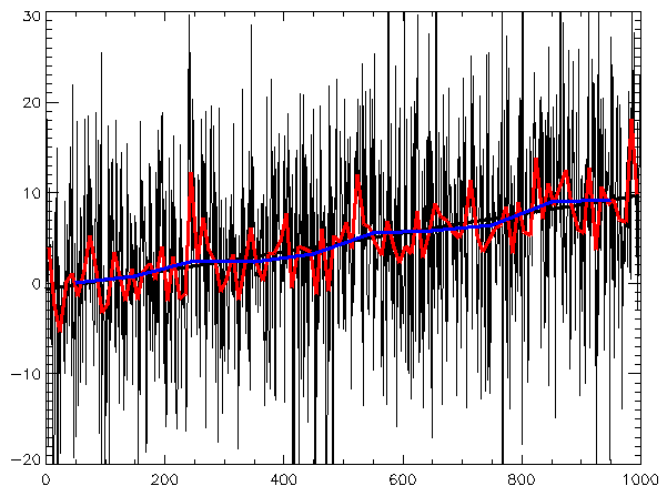
In mathematics, a time series is a series of data points indexed (or listed or graphed) in time order. Most commonly, a time series is a sequence taken at successive equally spaced points in time. Thus it is a sequence of discrete-time data. Examples of time series are heights of ocean tides, counts of sunspots, and the daily closing value of the Dow Jones Industrial Average. A time series is very frequently plotted via a run chart (which is a temporal line chart). Time series are used in statistics, signal processing, pattern recognition, econometrics, mathematical finance, weather forecasting, earthquake prediction, electroencephalography, control engineering, astronomy, communications engineering, and largely in any domain of applied science and engineering which involves temporal measurements. Time series ''analysis'' comprises methods for analyzing time series data in order to extract meaningful statistics and other characteristics of the data. Time series ''for ... [...More Info...] [...Related Items...] OR: [Wikipedia] [Google] [Baidu] |
John Denis Sargan
John Denis Sargan, FBA (23 August 1924 – 13 April 1996) was a British econometrician who specialized in the analysis of economic time-series. Sargan was born in Doncaster, Yorkshire in 1924, and was educated at Doncaster Grammar School and St John's College, Cambridge. He made many contributions, notably in instrumental variables estimation, Edgeworth expansions for the distributions of econometric estimators, identification conditions in simultaneous equations models, asymptotic tests for overidentifying restrictions in homoskedastic equations and exact tests for unit roots in autoregressive and moving average models. At the LSE, Sargan was Professor of Econometrics from 1964–1984.https://www.independent.co.uk/news/people/obituary--professor-denis-sargan-1305657.html Obituary: Professor Denis Sargan Friday, 19 April 1996 Sargan was President of the Econometric Society, a Fellow of the British Academy and an (honorary foreign) member of the American Academy of Arts a ... [...More Info...] [...Related Items...] OR: [Wikipedia] [Google] [Baidu] |
Average Propensity To Consume
Average propensity to consume (as well as the marginal propensity to consume) is a concept developed by John Maynard Keynes to analyze the consumption function, which is a formula where total consumption expenditures (C) of a household consist of autonomous consumption (Ca) and income (Y) (or disposable income (YD)) multiplied by marginal propensity to consume (c or MPC). According to Keynes, the individual´s real income determines saving and consumption decisions. Consumption function: C=+cY The average propensity to consume is referred to as the percentage of income spent on goods and services. It is the proportion of income that is consumed and it is calculated by dividing total consumption expenditure (C) by total income (Y): APC=\frac=\frac+c It can be also explained as spending on every monetary unit of income. Moreover Keynes´s theory claims that wealthier people spend less of their income on consumption than less wealthy people. This is caused by autonomous consumptio ... [...More Info...] [...Related Items...] OR: [Wikipedia] [Google] [Baidu] |
Permanent Income Hypothesis
The permanent income hypothesis (PIH) is a model in the field of economics to explain the formation of consumption patterns. It suggests consumption patterns are formed from future expectations and consumption smoothing. The theory was developed by Milton Friedman and published in his ''A Theory of Consumption Function'', published in 1957 and subsequently formalized by Robert Hall in a rational expectations model. Originally applied to consumption and income, the process of future expectations is thought to influence other phenomena. In its simplest form, the hypothesis states changes in permanent income (human capital, property, assets), rather than changes in temporary income (unexpected income), are what drive changes in consumption. The formation of consumption patterns opposite to predictions was an outstanding problem faced by the Keynesian orthodoxy. Friedman's predictions of consumption smoothing, where people spread out transitory changes in income over time, depar ... [...More Info...] [...Related Items...] OR: [Wikipedia] [Google] [Baidu] |
Vector Autoregression
Vector autoregression (VAR) is a statistical model used to capture the relationship between multiple quantities as they change over time. VAR is a type of stochastic process model. VAR models generalize the single-variable (univariate) autoregressive model by allowing for multivariate time series. VAR models are often used in economics and the natural sciences. Like the autoregressive model, each variable has an equation modelling its evolution over time. This equation includes the variable's lagged (past) values, the lagged values of the other variables in the model, and an error term. VAR models do not require as much knowledge about the forces influencing a variable as do structural models with simultaneous equations. The only prior knowledge required is a list of variables which can be hypothesized to affect each other over time. Specification Definition A VAR model describes the evolution of a set of ''k'' variables, called ''endogenous variables'', over time. Each pe ... [...More Info...] [...Related Items...] OR: [Wikipedia] [Google] [Baidu] |
Granger Causality
The Granger causality test is a statistical hypothesis test for determining whether one time series is useful in forecasting another, first proposed in 1969. Ordinarily, regressions reflect "mere" correlations, but Clive Granger argued that causality in economics could be tested for by measuring the ability to predict the future values of a time series using prior values of another time series. Since the question of "true causality" is deeply philosophical, and because of the post hoc ergo propter hoc fallacy of assuming that one thing preceding another can be used as a proof of causation, econometricians assert that the Granger test finds only "predictive causality". Using the term "causality" alone is a misnomer, as Granger-causality is better described as "precedence", or, as Granger himself later claimed in 1977, "temporally related". Rather than testing whether ''X'' ''causes'' Y, the Granger causality tests whether X ''forecasts'' ''Y.'' A time series ''X'' is said to Gr ... [...More Info...] [...Related Items...] OR: [Wikipedia] [Google] [Baidu] |
Statistical Power
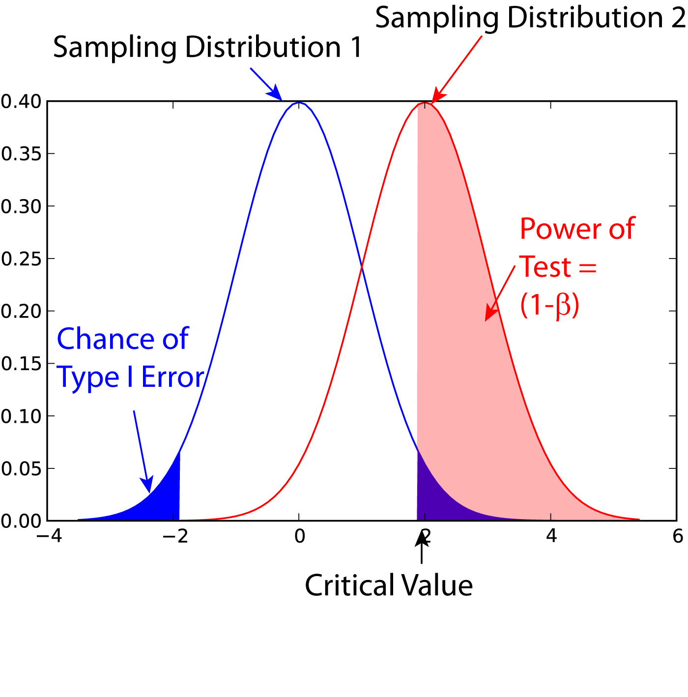
In statistics, the power of a binary hypothesis test is the probability that the test correctly rejects the null hypothesis (H_0) when a specific alternative hypothesis (H_1) is true. It is commonly denoted by 1-\beta, and represents the chances of a true positive detection conditional on the actual existence of an effect to detect. Statistical power ranges from 0 to 1, and as the power of a test increases, the probability \beta of making a type II error by wrongly failing to reject the null hypothesis decreases. Notation This article uses the following notation: * ''β'' = probability of a Type II error, known as a "false negative" * 1 − ''β'' = probability of a "true positive", i.e., correctly rejecting the null hypothesis. "1 − ''β''" is also known as the power of the test. * ''α'' = probability of a Type I error, known as a "false positive" * 1 − ''α'' = probability of a "true negative", i.e., correctly not rejecting the null hypothesis Description For a ... [...More Info...] [...Related Items...] OR: [Wikipedia] [Google] [Baidu] |
Consistent Estimator
In statistics, a consistent estimator or asymptotically consistent estimator is an estimator—a rule for computing estimates of a parameter ''θ''0—having the property that as the number of data points used increases indefinitely, the resulting sequence of estimates converges in probability to ''θ''0. This means that the distributions of the estimates become more and more concentrated near the true value of the parameter being estimated, so that the probability of the estimator being arbitrarily close to ''θ''0 converges to one. In practice one constructs an estimator as a function of an available sample of size ''n'', and then imagines being able to keep collecting data and expanding the sample ''ad infinitum''. In this way one would obtain a sequence of estimates indexed by ''n'', and consistency is a property of what occurs as the sample size “grows to infinity”. If the sequence of estimates can be mathematically shown to converge in probability to the true value ' ... [...More Info...] [...Related Items...] OR: [Wikipedia] [Google] [Baidu] |
Ordinary Least Squares
In statistics, ordinary least squares (OLS) is a type of linear least squares method for choosing the unknown parameters in a linear regression model (with fixed level-one effects of a linear function of a set of explanatory variables) by the principle of least squares: minimizing the sum of the squares of the differences between the observed dependent variable (values of the variable being observed) in the input dataset and the output of the (linear) function of the independent variable. Geometrically, this is seen as the sum of the squared distances, parallel to the axis of the dependent variable, between each data point in the set and the corresponding point on the regression surface—the smaller the differences, the better the model fits the data. The resulting estimator can be expressed by a simple formula, especially in the case of a simple linear regression, in which there is a single regressor on the right side of the regression equation. The OLS estimator is con ... [...More Info...] [...Related Items...] OR: [Wikipedia] [Google] [Baidu] |
Unit Root
In probability theory and statistics, a unit root is a feature of some stochastic processes (such as random walks) that can cause problems in statistical inference involving time series models. A linear stochastic process has a unit root if 1 is a root of the process's characteristic equation. Such a process is non-stationary but does not always have a trend. If the other roots of the characteristic equation lie inside the unit circle—that is, have a modulus ( absolute value) less than one—then the first difference of the process will be stationary; otherwise, the process will need to be differenced multiple times to become stationary. If there are ''d'' unit roots, the process will have to be differenced ''d'' times in order to make it stationary. Due to this characteristic, unit root processes are also called difference stationary. Unit root processes may sometimes be confused with trend-stationary processes; while they share many properties, they are different in ... [...More Info...] [...Related Items...] OR: [Wikipedia] [Google] [Baidu] |
Stationary Process
In mathematics and statistics, a stationary process (or a strict/strictly stationary process or strong/strongly stationary process) is a stochastic process whose unconditional joint probability distribution does not change when shifted in time. Consequently, parameters such as mean and variance also do not change over time. If you draw a line through the middle of a stationary process then it should be flat; it may have 'seasonal' cycles, but overall it does not trend up nor down. Since stationarity is an assumption underlying many statistical procedures used in time series analysis, non-stationary data are often transformed to become stationary. The most common cause of violation of stationarity is a trend in the mean, which can be due either to the presence of a unit root or of a deterministic trend. In the former case of a unit root, stochastic shocks have permanent effects, and the process is not mean-reverting. In the latter case of a deterministic trend, the process is cal ... [...More Info...] [...Related Items...] OR: [Wikipedia] [Google] [Baidu] |


