|
Diffusion Equation
The diffusion equation is a parabolic partial differential equation. In physics, it describes the macroscopic behavior of many micro-particles in Brownian motion, resulting from the random movements and collisions of the particles (see Fick's laws of diffusion). In mathematics, it is related to Markov processes, such as random walks, and applied in many other fields, such as materials science, information theory, and biophysics. The diffusion equation is a special case of the convection–diffusion equation when bulk velocity is zero. It is equivalent to the heat equation under some circumstances. Statement The equation is usually written as: \frac = \nabla \cdot \big D(\phi,\mathbf) \ \nabla\phi(\mathbf,t) \big where is the density of the diffusing material at location and time and is the collective diffusion coefficient for density at location ; and represents the vector differential operator del. If the diffusion coefficient depends on the density then the equatio ... [...More Info...] [...Related Items...] OR: [Wikipedia] [Google] [Baidu] |
Parabolic Partial Differential Equation
A parabolic partial differential equation is a type of partial differential equation (PDE). Parabolic PDEs are used to describe a wide variety of time-dependent phenomena in, for example, engineering science, quantum mechanics and financial mathematics. Examples include the heat equation, Schrödinger_equation#Time-dependent_equation, time-dependent Schrödinger equation and the Black–Scholes equation. Definition To define the simplest kind of parabolic PDE, consider a real-valued function u(x, y) of two independent real variables, x and y. A Partial differential equation#Classification, second-order, linear, constant-coefficient PDE for u takes the form :Au_ + 2Bu_ + Cu_ + Du_x + Eu_y + F = 0, where the subscripts denote the first- and second-order partial derivatives with respect to x and y. The PDE is classified as ''parabolic'' if the coefficients of the principal part (i.e. the terms containing the second derivatives of u) satisfy the condition :B^2 - AC = 0. Usual ... [...More Info...] [...Related Items...] OR: [Wikipedia] [Google] [Baidu] |
Adolf Fick
Adolf Eugen Fick (3 September 1829 – 21 August 1901) was a German-born physician and physiologist. Early life and education Fick began his work in the formal study of mathematics and physics before realising an aptitude for medicine. He then earned his doctorate in medicine from the University of Marburg in 1851. As a fresh medical graduate, he began his work as a prosector.The Virtual Laboratory: Fick, Adolf Eugen accessed 5 February 2006 He died in at age 71. Career In 1855, he introduced Fick's laws of diffusion, which govern the |
Structure Tensor
In mathematics, the structure tensor, also referred to as the second-moment matrix, is a matrix (mathematics), matrix derived from the gradient of a function (mathematics), function. It describes the distribution of the gradient in a specified neighborhood around a point and makes the information invariant to the observing coordinates. The structure tensor is often used in image processing and computer vision. J. Bigun and G. Granlund (1986), ''Optimal Orientation Detection of Linear Symmetry''. Tech. Report LiTH-ISY-I-0828, Computer Vision Laboratory, Linkoping University, Sweden 1986; Thesis Report, Linkoping studies in science and technology No. 85, 1986. The 2D structure tensor Continuous version For a function I of two variables , the structure tensor is the 2×2 matrix S_w(p) = \begin \int w(r) (I_x(p-r))^2\,dr & \int w(r) I_x(p-r)I_y(p-r)\,dr \\[10pt] \int w(r) I_x(p-r)I_y(p-r)\,dr & \int w(r) (I_y(p-r))^2\,dr \end where I_x and I_y are the partial derivatives of I ... [...More Info...] [...Related Items...] OR: [Wikipedia] [Google] [Baidu] |
Eigenvectors
In linear algebra, an eigenvector ( ) or characteristic vector is a Vector (mathematics and physics), vector that has its direction (geometry), direction unchanged (or reversed) by a given linear map, linear transformation. More precisely, an eigenvector \mathbf v of a linear transformation T is scalar multiplication, scaled by a constant factor \lambda when the linear transformation is applied to it: T\mathbf v=\lambda \mathbf v. The corresponding eigenvalue, characteristic value, or characteristic root is the multiplying factor \lambda (possibly a negative number, negative or complex number, complex number). Euclidean vector, Geometrically, vectors are multi-dimensional quantities with magnitude and direction, often pictured as arrows. A linear transformation Rotation (mathematics), rotates, Scaling (geometry), stretches, or Shear mapping, shears the vectors upon which it acts. A linear transformation's eigenvectors are those vectors that are only stretched or shrunk, with nei ... [...More Info...] [...Related Items...] OR: [Wikipedia] [Google] [Baidu] |
Transpose
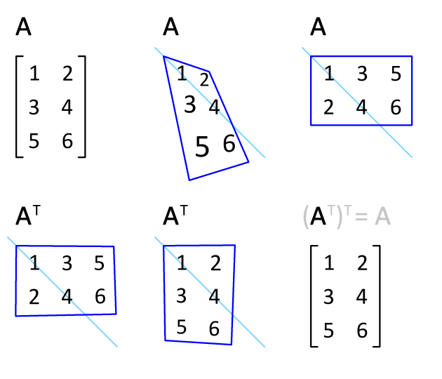
In linear algebra, the transpose of a Matrix (mathematics), matrix is an operator which flips a matrix over its diagonal; that is, it switches the row and column indices of the matrix by producing another matrix, often denoted by (among other notations). The transpose of a matrix was introduced in 1858 by the British mathematician Arthur Cayley. Transpose of a matrix Definition The transpose of a matrix , denoted by , , , A^, , , or , may be constructed by any one of the following methods: #Reflection (mathematics), Reflect over its main diagonal (which runs from top-left to bottom-right) to obtain #Write the rows of as the columns of #Write the columns of as the rows of Formally, the -th row, -th column element of is the -th row, -th column element of : :\left[\mathbf^\operatorname\right]_ = \left[\mathbf\right]_. If is an matrix, then is an matrix. In the case of square matrices, may also denote the th power of the matrix . For avoiding a possibl ... [...More Info...] [...Related Items...] OR: [Wikipedia] [Google] [Baidu] |
Tensor
In mathematics, a tensor is an algebraic object that describes a multilinear relationship between sets of algebraic objects associated with a vector space. Tensors may map between different objects such as vectors, scalars, and even other tensors. There are many types of tensors, including scalars and vectors (which are the simplest tensors), dual vectors, multilinear maps between vector spaces, and even some operations such as the dot product. Tensors are defined independent of any basis, although they are often referred to by their components in a basis related to a particular coordinate system; those components form an array, which can be thought of as a high-dimensional matrix. Tensors have become important in physics because they provide a concise mathematical framework for formulating and solving physics problems in areas such as mechanics ( stress, elasticity, quantum mechanics, fluid mechanics, moment of inertia, ...), electrodynamics ( electromagnetic ten ... [...More Info...] [...Related Items...] OR: [Wikipedia] [Google] [Baidu] |
Trace (linear Algebra)
In linear algebra, the trace of a square matrix , denoted , is the sum of the elements on its main diagonal, a_ + a_ + \dots + a_. It is only defined for a square matrix (). The trace of a matrix is the sum of its eigenvalues (counted with multiplicities). Also, for any matrices and of the same size. Thus, similar matrices have the same trace. As a consequence, one can define the trace of a linear operator mapping a finite-dimensional vector space into itself, since all matrices describing such an operator with respect to a basis are similar. The trace is related to the derivative of the determinant (see Jacobi's formula). Definition The trace of an square matrix is defined as \operatorname(\mathbf) = \sum_^n a_ = a_ + a_ + \dots + a_ where denotes the entry on the row and column of . The entries of can be real numbers, complex numbers, or more generally elements of a field . The trace is not defined for non-square matrices. Example Let be a matrix, with \m ... [...More Info...] [...Related Items...] OR: [Wikipedia] [Google] [Baidu] |
Product Rule
In calculus, the product rule (or Leibniz rule or Leibniz product rule) is a formula used to find the derivatives of products of two or more functions. For two functions, it may be stated in Lagrange's notation as (u \cdot v)' = u ' \cdot v + u \cdot v' or in Leibniz's notation as \frac (u\cdot v) = \frac \cdot v + u \cdot \frac. The rule may be extended or generalized to products of three or more functions, to a rule for higher-order derivatives of a product, and to other contexts. Discovery Discovery of this rule is credited to Gottfried Leibniz, who demonstrated it using "infinitesimals" (a precursor to the modern differential). (However, J. M. Child, a translator of Leibniz's papers, argues that it is due to Isaac Barrow.) Here is Leibniz's argument: Let ''u'' and ''v'' be functions. Then ''d(uv)'' is the same thing as the difference between two successive ''uvs; let one of these be ''uv'', and the other ''u+du'' times ''v+dv''; then: \begin d(u\cdot v) & = (u + d ... [...More Info...] [...Related Items...] OR: [Wikipedia] [Google] [Baidu] |
Random Walk
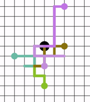
In mathematics, a random walk, sometimes known as a drunkard's walk, is a stochastic process that describes a path that consists of a succession of random steps on some Space (mathematics), mathematical space. An elementary example of a random walk is the random walk on the integer number line \mathbb Z which starts at 0, and at each step moves +1 or −1 with equal probability. Other examples include the path traced by a molecule as it travels in a liquid or a gas (see Brownian motion), the search path of a foraging animal, or the price of a fluctuating random walk hypothesis, stock and the financial status of a gambler. Random walks have applications to engineering and many scientific fields including ecology, psychology, computer science, physics, chemistry, biology, economics, and sociology. The term ''random walk'' was first introduced by Karl Pearson in 1905. Realizations of random walks can be obtained by Monte Carlo Simulation, Monte Carlo simulation. Lattice random ... [...More Info...] [...Related Items...] OR: [Wikipedia] [Google] [Baidu] |
Gaussian Kernel
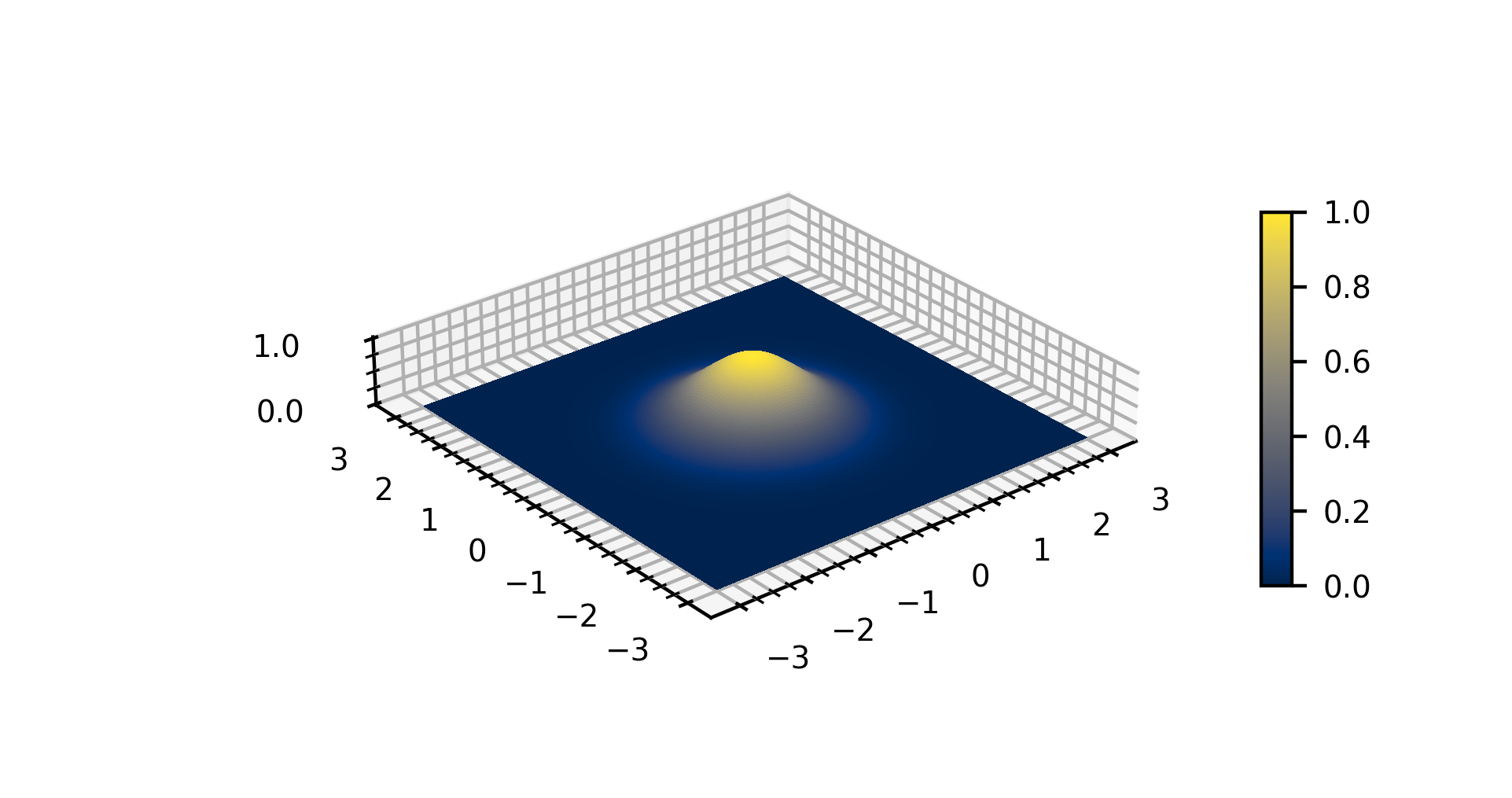
In mathematics, a Gaussian function, often simply referred to as a Gaussian, is a function of the base form f(x) = \exp (-x^2) and with parametric extension f(x) = a \exp\left( -\frac \right) for arbitrary real constants , and non-zero . It is named after the mathematician Carl Friedrich Gauss. The graph of a Gaussian is a characteristic symmetric " bell curve" shape. The parameter is the height of the curve's peak, is the position of the center of the peak, and (the standard deviation, sometimes called the Gaussian RMS width) controls the width of the "bell". Gaussian functions are often used to represent the probability density function of a normally distributed random variable with expected value and variance . In this case, the Gaussian is of the form g(x) = \frac \exp\left( -\frac \frac \right). Gaussian functions are widely used in statistics to describe the normal distributions, in signal processing to define Gaussian filters, in image processing where two-dimens ... [...More Info...] [...Related Items...] OR: [Wikipedia] [Google] [Baidu] |
Discrete Gaussian Kernel
In the areas of computer vision, image analysis and signal processing, the notion of scale-space representation is used for processing measurement data at multiple scales, and specifically enhance or suppress image features over different ranges of scale (see the article on scale space). A special type of scale-space representation is provided by the Gaussian scale space, where the image data in ''N'' dimensions is subjected to smoothing by Gaussian convolution. Most of the theory for Gaussian scale space deals with continuous images, whereas one when implementing this theory will have to face the fact that most measurement data are discrete. Hence, the theoretical problem arises concerning how to discretize the continuous theory while either preserving or well approximating the desirable theoretical properties that lead to the choice of the Gaussian kernel (see the article on scale-space axioms). This article describes basic approaches for this that have been developed in the liter ... [...More Info...] [...Related Items...] OR: [Wikipedia] [Google] [Baidu] |
Green's Function
In mathematics, a Green's function (or Green function) is the impulse response of an inhomogeneous linear differential operator defined on a domain with specified initial conditions or boundary conditions. This means that if L is a linear differential operator, then * the Green's function G is the solution of the equation where \delta is Dirac's delta function; * the solution of the initial-value problem L y = f is the convolution Through the superposition principle, given a linear ordinary differential equation (ODE), one can first solve for each , and realizing that, since the source is a sum of delta functions, the solution is a sum of Green's functions as well, by linearity of . Green's functions are named after the British mathematician George Green, who first developed the concept in the 1820s. In the modern study of linear partial differential equations, Green's functions are studied largely from the point of view of fundamental solutions instead. Under many ... [...More Info...] [...Related Items...] OR: [Wikipedia] [Google] [Baidu] |


