Lineweaver–Burk plot

In biochemistry, the Lineweaver–Burk plot (or double reciprocal plot) is a graphical representation of the Michaelis–Menten equation of enzyme kinetics, described by Hans Lineweaver and Dean Burk in 1934.

The double reciprocal plot distorts the error structure of the data, and is therefore not the most accurate tool for the determination of enzyme kinetic parameters. While the Lineweaver–Burk plot has historically been used for evaluation of the parameters, together with the alternative linear forms of the Michaelis–Menten equation such as the Hanes–Woolf plot or Eadie–Hofstee plot, all linearized forms of the Michaelis–Menten equation should be avoided to calculate the kinetic parameters. Properly weighted non-linear regression methods are significantly more accurate and have become generally accessible with the universal availability of desktop computers.

Definitions

The Lineweaver–Burk plot derives from a transformation of the Michaelis–Menten equation,

:$v = \frac$

in which the rate $v$ is a function of the substrate concentration $a$ and two parameters $V$, the limiting rate, and $K_\mathrm$, the Michaelis constant. Taking reciprocals of both sides of this equation it becomes as follows:

:$\frac = \frac + \frac \cdot \frac$

Thus plotting $1/v$ against $1/a$ generates a straight line with ordinate (y) intercept $1/V$, abscissa (x) intercept $-1/K_\mathrm$ and slope $K_\mathrm/V$.

Applications

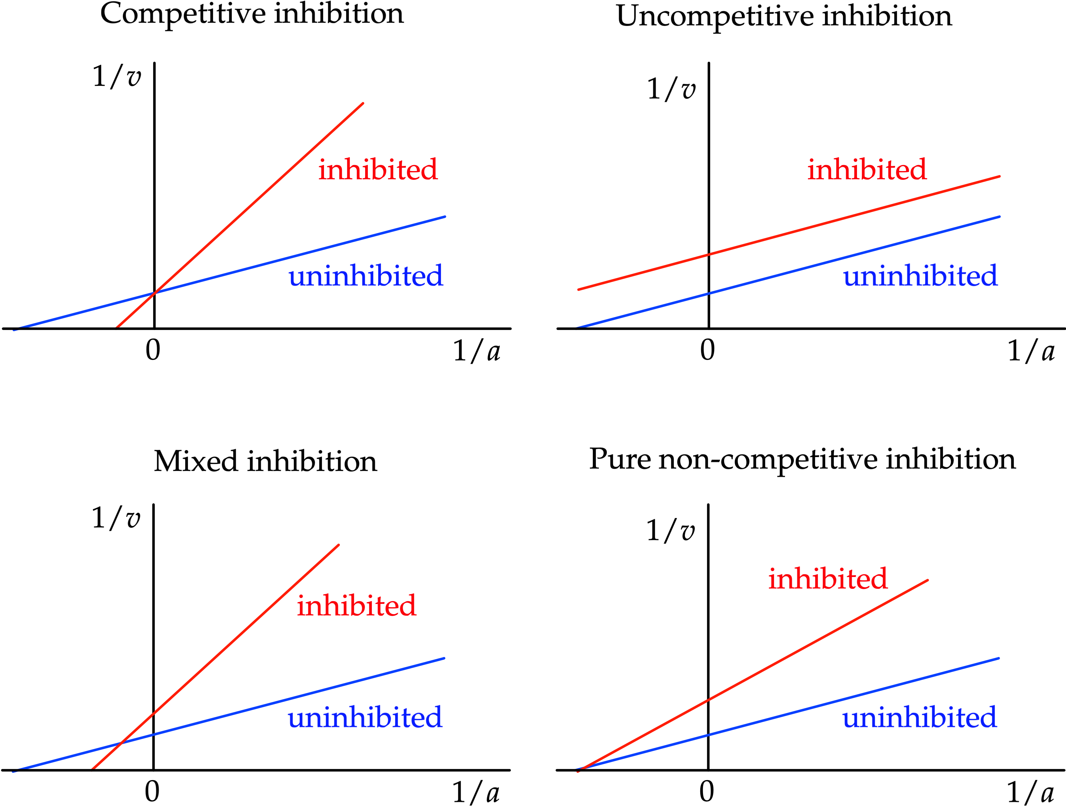
When used for determining the type of enzyme inhibition, the Lineweaver–Burk plot can distinguish between competitive, pure non-competitive and uncompetitive inhibitors. The various modes of inhibition can be compared to the uninhibited reaction.

Competitive inhibition

The apparent value of $V$ is unaffected by competitive inhibitors. Therefore competitive inhibitors have the same intercept on the ordinate as uninhibited enzymes.

Competitive inhibition increases the apparent value of $K_\mathrm$, or lowers substrate affinity. Graphically this can be seen as the inhibited enzyme having a larger intercept on the abscissa.

Pure non-competitive inhibition

With pure noncompetitive inhibition the apparent value of $V$ is decreased. This can be seen on the Lineweaver–Burk plot as an increased ordinate intercept with no effect on the abscissa intercept $-1/K_\mathrm$, as pure noncompetitive inhibition does not effect substrate affinity.

Mixed inhibition

Pure noncompetitive inhibition is rare, and mixed inhibition is much more common. In mixed inhibition the apparent value of $V$ is decreased, and that of $K_\mathrm$ is changed—usually increased, meaning that the affinity usually decreases with mixed inhibition.

Cleland recognized that pure noncompetitive inhibition was very rare in practice, occurring mainly with effects of protons and some metal ions, and he redefined ''noncompetitive'' to mean ''mixed''. Many authors have followed him in this respect, but not all.

Uncompetitive inhibition

The apparent value of $V$ decreases with uncompetitive inhibition, with that of $V/K_\mathrm$. This can be seen on the Lineweaver–Burk plot as an increased intercept on the ordinate with no change in slope.

Substrate affinity increases with uncompetitive inhibition, or lowers the apparent value of $K_\mathrm$. Graphically uncompetitive inhibition can be identified in the plot parallel lines for the different concentrations of inhibitor..

Shortcomings

The Lineweaver–Burk plot does a poor job of visualizing experimental error. Specifically, if the errors $\varepsilon (v)$ have uniform standard errors, then those of $1/v$ vary over a very wide range, as can be seen from the following example:

: If $v = 1 \pm 0.1$ then the range of $1/v$ is 0.91–1.11, approximately 20%
: If $v = 10 \pm 0.1$ (same standard deviation) then the range of $1/v$ is 0.0990–0.1001, approximately 1%.

Lineweaver and Burk were aware of this problem, and after investigating the error distribution experimentally, finding a uniform standard deviation in $v$, they consulted the eminent statistician W. Edwards Deming. In the light of his advice they used weights of $v^4$ for fitting their $1/v$. This aspect of their paper has been almost universally ignored by people who refer to the "method of Lineweaver and Burk."

The values measured at low $a$, and hence large values of $1/a$ lead to points on the far right of the plot and have a large effect on the slope of the line, and thus in particular on the value of $K_\mathrm$.

See also

* Michaelis–Menten kinetics
* Eadie–Hofstee plot
* Hanes–Woolf plot
* Direct linear plot

References

External links

NIH guide
enzyme assay development and analysis

{{DEFAULTSORT:Lineweaver-Burk plot
Plots (graphics)
Enzyme kinetics