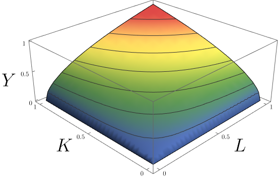
Cobb–Douglas Production Function

In economics and econometrics, the Cobb–Douglas production function is a particular functional form of the production function, widely used to represent the technological relationship between the amounts of two or more inputs (particularly physical capital and labor) and the amount of output that can be produced by those inputs. The Cobb–Douglas form was developed and tested against statistical evidence by Charles Cobb and Paul Douglas between 1927 and 1947; according to Douglas, the functional form itself was developed earlier by Philip Wicksteed.

Formulation

In its most standard form for production of a single good with two factors, the function is given by:

: $Y(L,K)=AL^\beta K^\alpha$

where:
* ''Y'' = total production (the real value of all goods produced in a year or 365.25 days)
* ''L'' = labour input (person-hours worked in a year or 365.25 days)
* ''K'' = capital input (a measure of all machinery, equipment, and buildings; the value of capital input divided by the price of capital)
* ''A'' = total factor productivity
* $0<\alpha<1$ and $0<\beta<1$ are the output elasticities of capital and labor, respectively. These values are constants determined by available technology.

Capital and labour are the two "factors of production" of the Cobb–Douglas production function.

History

Paul Douglas explained that his first formulation of the Cobb–Douglas production function was developed in 1927; when seeking a functional form to relate estimates he had calculated for workers and capital, he spoke with mathematician and colleague Charles Cobb, who suggested a function of the form , previously used by Knut Wicksell, Philip Wicksteed, and Léon Walras, although Douglas only acknowledges Wicksteed and Walras for their contributions. Not long after Knut Wicksell's death in 1926, Paul Douglas and Charles Cobb implemented the Cobb–Douglas function in their work covering the subject manner of producer theory for the first time. Estimating this using least squares, he obtained a result for the exponent of labour of 0.75—which was subsequently confirmed by the National Bureau of Economic Research to be 0.741. Later work in the 1940s prompted them to allow for the exponents on ''K'' and ''L'' to vary, resulting in estimates that subsequently proved to be very close to improved measure of productivity developed at that time.

A major criticism at the time was that estimates of the production function, although seemingly accurate, were based on such sparse data that it was hard to give them much credibility. Douglas remarked "I must admit I was discouraged by this criticism and thought of giving up the effort, but there was something which told me I should hold on." The breakthrough came in using US census data, which was cross-sectional and provided a large number of observations. Douglas presented the results of these findings, along with those for other countries, at his 1947 address as president of the American Economic Association. Shortly afterwards, Douglas went into politics and was stricken by ill health—resulting in little further development on his side. However, two decades later, his production function was widely used, being adopted by economists such as Paul Samuelson and Robert Solow. The Cobb–Douglas production function is especially notable for being the first time an aggregate or economy-wide production function had been developed, estimated, and then presented to the profession for analysis; it marked a landmark change in how economists approached macroeconomics from a microeconomics perspective.

Positivity of marginal products

The marginal product of a factor of production is the change in output when that factor of production changes, holding constant all the other factors of production as well as the total factor productivity.

The marginal product of capital, $MPK$ corresponds to the first derivative of the production function with respect to capital:

: $MPK=\frac = \alpha A L^\beta K^ = \alpha \frac = \alpha \frac$

Because $\alpha>0$ (and $Y>0, K>0$ as well), we find out that the marginal product of capital is always positive; that is, increasing capital leads to an increase in output.

We also find that increasing the total factor productivity $A$ increases the marginal product of capital.

An analogous reasoning holds for labor.

Law of diminishing returns

Taking the derivative of the marginal product of capital with respect to capital (i.e., taking the second derivative of the production function with respect to capital), we have:

: $\frac = \frac = \frac ( A L^\beta \alpha K^ ) = A L^\beta \alpha (\alpha-1) K^ = \alpha (\alpha-1) A L^\beta \frac = \alpha (\alpha-1) \frac$

Because $\alpha<1$, then $\alpha-1<0$ and so $\dfrac<0$.

Thus, this function satisfies the law of "diminishing returns"; that is, the marginal product of capital, while always positive, is declining. As capital increases (holding labor and total factor productivity constant), the output increases but at a diminishing rate.

A similar reasoning holds for labor.

Cross derivatives

We can study what happens to the marginal product of capital when labor increases by taking the partial derivative of the marginal product of capital with respect to labor, that is, the cross-derivative of output with respect to capital and labor:

$\dfrac = \dfrac = \dfrac ( A L^\beta \alpha K^ ) = A \beta L^ \alpha K^ = A \alpha \beta \dfrac = \alpha \beta \dfrac$

Since $\dfrac>0$, an increase in labor raises the marginal product of capital.

Returns to scale

Output elasticity measures the responsiveness of output to a change in levels of either labor or capital used in production, ceteris paribus. For example, if , a increase in capital usage would lead to approximately a increase in output.

Sometimes the term has a more restricted meaning, requiring that the function display constant returns to scale, meaning that increasing capital ''K'' and labor ''L'' by a factor ''k'' also increases output ''Y'' by the same factor, that is, $Y(kL,kK)=kY(L,K)$. This holds if $\alpha+\beta=1$.

If $\alpha+\beta<1$, then returns to scale are decreasing, meaning that an increase of capital ''K'' and labor ''L'' by a factor ''k'' will produce an increase in output ''Y'' smaller than a factor ''k'', that is Y(kL,kK).

If $\alpha+\beta>1$, then returns to scale are increasing, meaning that an increase in capital ''K'' and labor ''L'' by a factor ''k'' produce an increase in output ''Y'' greater than a factor ''k'', that is, $Y(kL,kK)>kY(L,K)$.

Remuneration under perfect competition

Under perfect competition, the factors of production are remunerated at their total marginal product.

Suppose that $Y=F(L,K) = L^\alpha K^$ where $0<\alpha<1$. In this case

$MP_L=\alpha L^ K^ = \alpha (\frac) ^$ and $MP_K=(1-\alpha) L^ K^ = (1-\alpha) (\frac) ^$.

Therefore, $Y=L\cdot MP_L + K\cdot MP_K = \alpha L^\alpha K^ + (1-\alpha)L^\alpha K^$. Dividing both sides by $Y=F(L,K) = L^\alpha K^$ we obtain that the remuneration of labor is $\alpha$ of the production and the remuneration of capital is $(1-\alpha)$ of the production.

Let us normalize the price of $Y$ to 1. In a competitive equilibrium the value of marginal product of a production factor equals its price or $P_Y\cdot MP_K = MP_K=w$ and similarly $MP_K= r$ where $w$ is the wage rate and $r$ is the price of capital, the real interest rate (assuming that capital fully depreciates after one period, otherwise, the price of capital is $r+\delta$ where $\delta$ is the depreciation rate of capital).

The total production can be written as follows: $Y=L\cdot w + K\cdot r$. That is, the value of production is divides between renumeration for labor and renumeration for capital.

Generalized form

In its generalized form, the Cobb–Douglas function models more than two goods. The Cobb–Douglas function may be written as

:$f(x)=A \prod_^n x_i^, \qquad x = (x_1, \ldots, x_n).$

where
* ''A'' is an efficiency parameter
* ''n'' is the total number of input variables (goods)
* are the (non-negative) quantities of good consumed, produced, etc.
* $\lambda_i$ is an elasticity parameter for good ''i''

Criticisms

The function has been criticised for its lack of foundation. Cobb and Douglas were influenced by statistical evidence that appeared to show that labor and capital shares of total output were constant over time in developed countries; they explained this by statistical fitting least-squares regression of their production function. It is now widely accepted that labor share is declining in industrialized economies. The production function contains a principal assumption that may not always provide the most accurate representation of a country's productive capabilities and supply-side efficiencies. This assumption is a "constant share of labor in output," which may not be effective when applied to cases of countries whose labor markets are growing at significant rates. Another issue within the fundamental composition the Cobb–Douglas production function is the presence of simultaneous equation bias. When competition is presumed, the simultaneous equation bias has impact on all function types involving firm decisions – including the Cobb–Douglas function. In some cases this simultaneous equation bias doesn't appear. However, it is apparent when least squares asymptotic approximations are used.

The Cobb–Douglas production function was not developed on the basis of any knowledge of engineering, technology, or management of the production process. This rationale may be true given the definition of the Capital term. Labor hours and Capital need a better definition. If capital is defined as a building, labor is already included in the development of that building. A building is composed of commodities, labor and risks and general conditions. It was instead developed because it had attractive mathematical characteristics, such as diminishing marginal returns to either factor of production and the property that the optimal expenditure shares on any given input of a firm operating a Cobb–Douglas technology are constant. Initially, there were no utility foundations for it. In the modern era, some economists try to build models up from individual agents acting, rather than imposing a functional form on an entire economy. The Cobb–Douglas production function, if properly defined, can be applied at a micro-economic level, up to a macro- economic level.

However, many modern authors have developed models which give microeconomically based Cobb–Douglas production functions, including many New Keynesian models. It is nevertheless a mathematical mistake to assume that just because the Cobb–Douglas function applies at the microeconomic level, it also always applies at the macroeconomic level. Similarly, it is not necessarily the case that a macro Cobb–Douglas applies at the disaggregated level. An early microfoundation of the aggregate Cobb–Douglas technology based on linear activities is derived in Houthakker (1955). The Cobb–Douglas production function is inconsistent with modern empirical estimates of the elasticity of substitution between capital and labor, which suggest that capital and labor are gross complements. A 2021 meta-analysis of 3186 estimates concludes that "the weight of evidence accumulated in the empirical literature emphatically rejects the Cobb–Douglas specification."

Cobb–Douglas utilities

The Cobb–Douglas function is often used as a utility function. Utility $\tilde$ is a function of the quantities $x_i$ of the $n$ goods consumed:

:$\tilde(x)= \prod_^n x_i^$

Utility functions represent ordinal preferences and do not have natural units, unlike production functions. As the result, a monotonic transformation of a utility function represents the same preferences. Unlike with a Cobb–Douglas production function, where the sum of the exponents determines the degree of economies of scale, the sum can be normalized to one for a utility function because normalization is a monotonic transformation of the original utility function. Thus, let us define $\lambda = \sum_^n \lambda_i$ and $\alpha_i = \frac$, so $\sum_^n \alpha_i = 1$, and write the utility function as:

:$u(x) = \prod_^n x_i^$

The consumer maximizes utility subject to the budget constraint that the cost of the goods is less than her wealth $w$. Letting $p_i$ denote the goods' prices, she solves:

:$\max_ \prod_^n x_i^ \quad \text \quad \sum_^n p_i x_i= w$
:The Marginal Rate of Substitution between each two goods is
:$MRS_=\frac=\Rightarrow p_j x_j=x_i$
:By inserting to the budget constrain we obtain
:
:$p_i x_i + \textstyle \sum_^n \displaystyle p_j x_j \frac = w$
:$\Rightarrow p_i x_i(1+\sum_^n \frac)=w \Rightarrow p_i x_i\frac =w \Rightarrow p_i x_i\frac =w$
:$\Rightarrow x_i^*=\frac \forall i$
:

Note that $p_i x^*_i = \alpha_i w$, the consumer spends fraction $\alpha_i$ of her wealth on good .

Also note that each good is affected solely by its own price. That is, any two goods are not substitute goods nor complementary goods. Namely, their cross elasticity equals to zero and the cross demand function of any good is described by a vertical line.

Finally, note that when the income increase by some percent the demand for the good increase by the same percent. That is, the elasticity of the demand with respect to income equals 1 and therefore, the Engel curve is a straight line starting from the origin.

Note that this is the solution for either $u(x)$ or $\tilde(x),$ since the same preferences generate the same demand.

The indirect utility function can be calculated by substituting the demands $x_i$ into the utility function. Define the constant $K= \prod_^n \alpha_i^$ and we get:

:$v(p,w) = \prod_^n \left( \frac \right)^ = \frac =K \left(\frac \right)$

which is a special case of the Gorman polar form. The expenditure function is the inverse of the indirect utility function:

:$e(p, u) = (1/K)\prod_^n p_i^ u$
:The Marshallian demand function that Cobb-Douglas utility function

Various representations of the production function

The Cobb–Douglas function form can be estimated as a linear relationship using the following expression:

:$\ln(Y) = a_0 + \sum_i a_i \ln(I_i)$
where
* $Y = \text$
* $I_i = \text$
* $a_i = \text$

The model can also be written as
:$Y = e^ (I_1)^ \cdot (I_2)^ \cdots$

As noted, the common Cobb–Douglas function used in macroeconomic modeling is
:$Y = K^\alpha L^\beta$

where ''K'' is capital and ''L'' is labor. When the model exponents sum to one, the production function is first-order homogeneous, which implies constant returns to scale—that is, if all inputs are scaled by a common factor greater than zero, output will be scaled by the same factor.

Relationship to the CES production function

The constant elasticity of substitution (CES) production function (in the two-factor case) is

:$Y = A \left ( \alpha K^\gamma + (1-\alpha) L^\gamma \right )^,$

in which the limiting case corresponds to a Cobb–Douglas function, $Y=AK^\alpha L^,$ with constant returns to scale.

To see this, the log of the CES function:

: $\ln(Y) = \ln(A) + \frac \ln \left (\alpha K^\gamma + (1-\alpha) L^\gamma \right )$

can be taken to the limit by applying L'Hôpital's rule:

:$\lim_ \ln(Y) = \ln(A) + \alpha \ln(K) + (1-\alpha) \ln(L).$

Therefore, $Y=AK^\alpha L^$.

Translog production function

The translog production function is an approximation of the CES function by a second-order Taylor polynomial in the variable $\gamma$ about $\gamma = 0$, i.e. the Cobb–Douglas case. The name translog stands for "transcendental logarithmic." It is often used in econometrics for the fact that it is linear in the parameters, which means ordinary least squares could be used if inputs could be assumed exogenous.

In the two-factor case above the translog production function is
: \begin
\ln(Y) &= \ln(A) + \alpha \ln(K) + (1-\alpha) \ln(L) + \frac \gamma \alpha (1 - \alpha) \left \ln(K) - \ln(L) \right2 \\
&= \ln(A) + a_K \ln(K) + a_L \ln(L) + b_ \ln^2(K) + b_ \ln^(L) + b_ \ln(K) \ln(L)
\end

where $a_K$, $a_L$, $b_$, $b_$, and $b_$ are defined appropriately. In the three factor case, the translog production function is:
:$\begin \ln(Y) & = \ln(A) + a_L\ln(L) + a_K\ln(K) + a_M\ln(M) + b_\ln^2(L) +b_\ln^2(K) + b_\ln^2(M) \\ & \qquad \qquad + b_\ln(L)\ln(K) + b_\ln(L)\ln(M) + b_\ln(K)\ln(M) \\ & = f(L,K,M). \end$
where $A$ = total factor productivity, $L$ = labor, $K$ = capital, $M$ = materials and supplies, and $Y$ = output.

See also

* Leontief production function
* Production–possibility frontier
* Production theory

References

Further reading

*

External links

Anatomy of Cobb–Douglas Type Production Functions in 3D

Analysis of the Cobb–Douglas as a utility function


Closed Form Solution for a firm with an N-input production function

{{DEFAULTSORT:Cobb-Douglas production function
Utility function types
1947 in economic history
Production economics