A* search algorithm on:
[Wikipedia]
[Google]
[Amazon]
A* (pronounced "A-star") is a
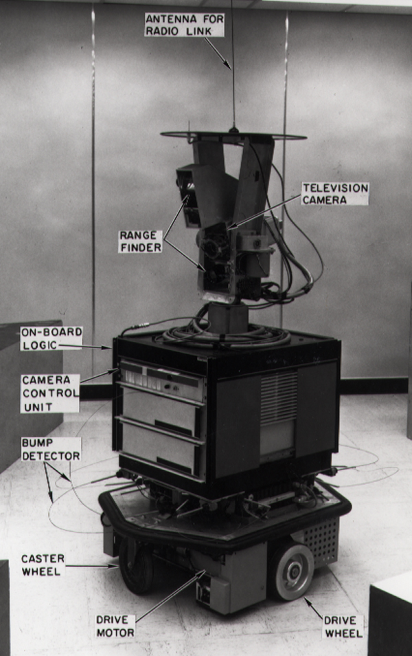 A* was created as part of the Shakey project, which had the aim of building a mobile robot that could plan its own actions. Nils Nilsson originally proposed using the Graph Traverser algorithm for Shakey's path planning. Graph Traverser is guided by a heuristic function , the estimated distance from node to the goal node: it entirely ignores , the distance from the start node to . Bertram Raphael suggested using the sum, . Peter Hart invented the concepts we now call admissibility and
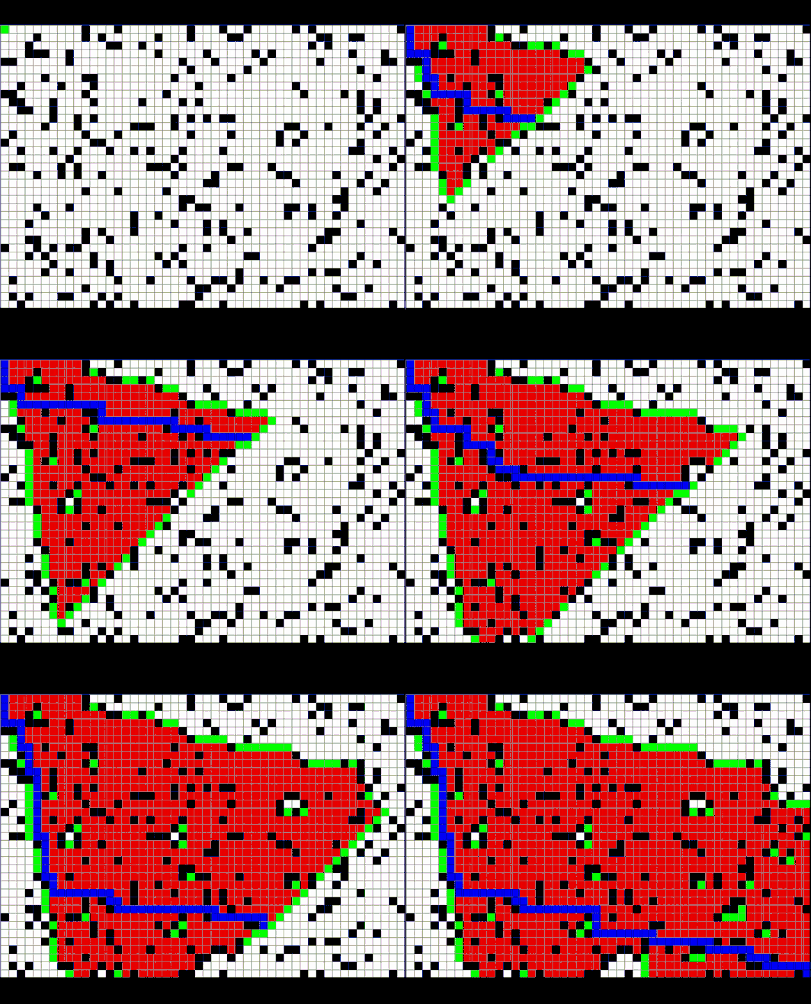 A* is an informed search algorithm, or a
function reconstruct_path(cameFrom, current)
total_path :=
while current in cameFrom.Keys:
current := cameFrom urrent total_path.prepend(current)
return total_path
// A* finds a path from start to goal.
// h is the heuristic function. h(n) estimates the cost to reach goal from node n.
function A_Star(start, goal, h)
// The set of discovered nodes that may need to be (re-)expanded.
// Initially, only the start node is known.
// This is usually implemented as a min-heap or priority queue rather than a hash-set.
openSet :=
// For node n, cameFrom is the node immediately preceding it on the cheapest path from the start
// to n currently known.
cameFrom := an empty map
// For node n, gScore is the currently known cost of the cheapest path from start to n.
gScore := map with default value of Infinity
gScore
Remark: In this pseudocode, if a node is reached by one path, removed from openSet, and subsequently reached by a cheaper path, it will be added to openSet again. This is essential to guarantee that the path returned is optimal if the heuristic function is admissible but not
graph traversal
In computer science, graph traversal (also known as graph search) refers to the process of visiting (checking and/or updating) each vertex in a graph. Such traversals are classified by the order in which the vertices are visited. Tree traversa ...
and pathfinding algorithm
In mathematics and computer science, an algorithm () is a finite sequence of Rigour#Mathematics, mathematically rigorous instructions, typically used to solve a class of specific Computational problem, problems or to perform a computation. Algo ...
that is used in many fields of computer science
Computer science is the study of computation, information, and automation. Computer science spans Theoretical computer science, theoretical disciplines (such as algorithms, theory of computation, and information theory) to Applied science, ...
due to its completeness, optimality, and optimal efficiency. Given a weighted graph
This is a glossary of graph theory. Graph theory is the study of graphs, systems of nodes or vertices connected in pairs by lines or edges.
Symbols
A
B
...
, a source node
In general, a node is a localized swelling (a "knot") or a point of intersection (a vertex).
Node may refer to:
In mathematics
* Vertex (graph theory), a vertex in a mathematical graph
*Vertex (geometry), a point where two or more curves, lines ...
and a goal node, the algorithm finds the shortest path
In graph theory, the shortest path problem is the problem of finding a path between two vertices (or nodes) in a graph such that the sum of the weights of its constituent edges is minimized.
The problem of finding the shortest path between two ...
(with respect to the given weights) from source to goal.
One major practical drawback is its space complexity
The space complexity of an algorithm or a data structure is the amount of memory space required to solve an instance of the computational problem as a function of characteristics of the input. It is the memory required by an algorithm until it exec ...
where is the depth of the shallowest solution (the length of the shortest path from the source node to any given goal node) and is the branching factor
In computing, tree data structures, and game theory, the branching factor is the number of children at each node, the outdegree. If this value is not uniform, an ''average branching factor'' can be calculated.
For example, in chess, if a "node ...
(the maximum number of successors for any given state), as it stores all generated nodes in memory. Thus, in practical travel-routing systems, it is generally outperformed by algorithms that can pre-process the graph to attain better performance, as well as by memory-bounded approaches; however, A* is still the best solution in many cases.
Peter Hart, Nils Nilsson and Bertram Raphael of Stanford Research Institute (now SRI International
SRI International (SRI) is a nonprofit organization, nonprofit scientific research, scientific research institute and organization headquartered in Menlo Park, California, United States. It was established in 1946 by trustees of Stanford Univer ...
) first published the algorithm in 1968.
It can be seen as an extension of Dijkstra's algorithm
Dijkstra's algorithm ( ) is an algorithm for finding the shortest paths between nodes in a weighted graph, which may represent, for example, a road network. It was conceived by computer scientist Edsger W. Dijkstra in 1956 and published three ...
. A* achieves better performance by using heuristics
A heuristic or heuristic technique (''problem solving'', '' mental shortcut'', ''rule of thumb'') is any approach to problem solving that employs a pragmatic method that is not fully optimized, perfected, or rationalized, but is nevertheless ...
to guide its search.
Compared to Dijkstra's algorithm, the A* algorithm only finds the shortest path from a specified source to a specified goal, and not the shortest-path tree from a specified source to all possible goals. This is a necessary trade-off
A trade-off (or tradeoff) is a situational decision that involves diminishing or losing on quality, quantity, or property of a set or design in return for gains in other aspects. In simple terms, a tradeoff is where one thing increases, and anoth ...
for using a specific-goal-directed heuristic
A heuristic or heuristic technique (''problem solving'', '' mental shortcut'', ''rule of thumb'') is any approach to problem solving that employs a pragmatic method that is not fully optimized, perfected, or rationalized, but is nevertheless ...
. For Dijkstra's algorithm, since the entire shortest-path tree is generated, every node is a goal, and there can be no specific-goal-directed heuristic.
History
 A* was created as part of the Shakey project, which had the aim of building a mobile robot that could plan its own actions. Nils Nilsson originally proposed using the Graph Traverser algorithm for Shakey's path planning. Graph Traverser is guided by a heuristic function , the estimated distance from node to the goal node: it entirely ignores , the distance from the start node to . Bertram Raphael suggested using the sum, . Peter Hart invented the concepts we now call admissibility and
 consistency
In deductive logic, a consistent theory is one that does not lead to a logical contradiction. A theory T is consistent if there is no formula \varphi such that both \varphi and its negation \lnot\varphi are elements of the set of consequences ...
of heuristic functions. A* was originally designed for finding least-cost paths when the cost of a path is the sum of its costs, but it has been shown that A* can be used to find optimal paths for any problem satisfying the conditions of a cost algebra.
The original 1968 A* paper contained a theorem stating that no A*-like algorithm could expand fewer nodes than A* if the heuristic function is consistent and A*'s tie-breaking rule is suitably chosen. A "correction" was published a few years later claiming that consistency was not required, but this was shown to be false in 1985 in Dechter and Pearl's definitive study of A*'s optimality (now called optimal efficiency), which gave an example of A* with a heuristic that was admissible but not consistent expanding arbitrarily more nodes than an alternative A*-like algorithm.
Description
 A* is an informed search algorithm, or a
 best-first search
Best-first search is a class of search algorithms which explores a graph by expanding the most promising node chosen according to a specified rule.
Judea Pearl described best-first search as estimating the promise of node ''n'' by a "heuristic eva ...
, meaning that it is formulated in terms of weighted graph
This is a glossary of graph theory. Graph theory is the study of graphs, systems of nodes or vertices connected in pairs by lines or edges.
Symbols
A
B
...
s: starting from a specific starting node
In general, a node is a localized swelling (a "knot") or a point of intersection (a vertex).
Node may refer to:
In mathematics
* Vertex (graph theory), a vertex in a mathematical graph
*Vertex (geometry), a point where two or more curves, lines ...
of a graph, it aims to find a path to the given goal node having the smallest cost (least distance travelled, shortest time, etc.). It does this by maintaining a tree
In botany, a tree is a perennial plant with an elongated stem, or trunk, usually supporting branches and leaves. In some usages, the definition of a tree may be narrower, e.g., including only woody plants with secondary growth, only ...
of paths originating at the start node and extending those paths one edge at a time until the goal node is reached.
At each iteration of its main loop, A* needs to determine which of its paths to extend. It does so based on the cost of the path and an estimate of the cost required to extend the path all the way to the goal. Specifically, A* selects the path that minimizes
:
where is the next node on the path, is the cost of the path from the start node to , and is a heuristic
A heuristic or heuristic technique (''problem solving'', '' mental shortcut'', ''rule of thumb'') is any approach to problem solving that employs a pragmatic method that is not fully optimized, perfected, or rationalized, but is nevertheless ...
function that estimates the cost of the cheapest path from to the goal. The heuristic function is problem-specific. If the heuristic function is admissible – meaning that it never overestimates the actual cost to get to the goal – A* is guaranteed to return a least-cost path from start to goal.
Typical implementations of A* use a priority queue
In computer science, a priority queue is an abstract data type similar to a regular queue (abstract data type), queue or stack (abstract data type), stack abstract data type.
In a priority queue, each element has an associated ''priority'', which ...
to perform the repeated selection of minimum (estimated) cost nodes to expand. This priority queue is known as the ''open set'', ''fringe'' or ''frontier''. At each step of the algorithm, the node with the lowest value is removed from the queue, the and values of its neighbors are updated accordingly, and these neighbors are added to the queue. The algorithm continues until a removed node (thus the node with the lowest value out of all fringe nodes) is a goal node. The value of that goal is then also the cost of the shortest path, since at the goal is zero in an admissible heuristic.
The algorithm described so far only gives the length of the shortest path. To find the actual sequence of steps, the algorithm can be easily revised so that each node on the path keeps track of its predecessor. After this algorithm is run, the ending node will point to its predecessor, and so on, until some node's predecessor is the start node.
As an example, when searching for the shortest route on a map, might represent the straight-line distance to the goal, since that is physically the smallest possible distance between any two points. For a grid map from a video game, using the Taxicab distance or the Chebyshev distance
In mathematics, Chebyshev distance (or Tchebychev distance), maximum metric, or L∞ metric is a metric defined on a real coordinate space where the distance between two points is the greatest of their differences along any coordinate dimensio ...
becomes better depending on the set of movements available (4-way or 8-way).
If the heuristic satisfies the additional condition for every edge of the graph (where denotes the length of that edge), then is called monotone, or consistent. With a consistent heuristic, A* is guaranteed to find an optimal path without processing any node more than once and A* is equivalent to running Dijkstra's algorithm
Dijkstra's algorithm ( ) is an algorithm for finding the shortest paths between nodes in a weighted graph, which may represent, for example, a road network. It was conceived by computer scientist Edsger W. Dijkstra in 1956 and published three ...
with the reduced cost
In linear programming, reduced cost, or opportunity cost, is the amount by which an objective function coefficient would have to improve (so increase for maximization problem, decrease for minimization problem) before it would be possible for a c ...
.
Pseudocode
The followingpseudocode
In computer science, pseudocode is a description of the steps in an algorithm using a mix of conventions of programming languages (like assignment operator, conditional operator, loop) with informal, usually self-explanatory, notation of actio ...
describes the algorithm:
tart
A tart is a baked dish consisting of a filling over a pastry base with an open top not covered with pastry. The pastry is usually shortcrust pastry; the filling may be sweet or savoury, though modern tarts are usually fruit-based, sometimes with ...
:= 0
// For node n, fScore := gScore + h(n). fScore represents our current best guess as to
// how cheap a path could be from start to finish if it goes through n.
fScore := map with default value of Infinity
fScoretart
A tart is a baked dish consisting of a filling over a pastry base with an open top not covered with pastry. The pastry is usually shortcrust pastry; the filling may be sweet or savoury, though modern tarts are usually fruit-based, sometimes with ...
:= h(start)
while openSet is not empty
// This operation can occur in O(Log(N)) time if openSet is a min-heap or a priority queue
current := the node in openSet having the lowest fScore[] value
if current = goal
return reconstruct_path(cameFrom, current)
openSet.Remove(current)
for each neighbor of current
// d(current,neighbor) is the weight of the edge from current to neighbor
// tentative_gScore is the distance from start to the neighbor through current
tentative_gScore := gScore urrent+ d(current, neighbor)
if tentative_gScore < gScore eighbor // This path to neighbor is better than any previous one. Record it!
cameFrom eighbor:= current
gScore eighbor:= tentative_gScore
fScore eighbor:= tentative_gScore + h(neighbor)
if neighbor not in openSet
openSet.add(neighbor)
// Open set is empty but goal was never reached
return failure
consistent
In deductive logic, a consistent theory is one that does not lead to a logical contradiction. A theory T is consistent if there is no formula \varphi such that both \varphi and its negation \lnot\varphi are elements of the set of consequences ...
. If the heuristic is consistent, when a node is removed from openSet the path to it is guaranteed to be optimal so the test ‘tentative_gScore < gScore eighbor/code>’ will always fail if the node is reached again. The pseudocode implemented here is sometimes called the ''graph-search'' version of A*. This is in contrast with the version without the ‘tentative_gScore < gScore eighbor/code>’ test to add nodes back to openSet, which is sometimes called the ''tree-search'' version of A* and require a consistent heuristic to guarantee optimality.
Example
An example of an A* algorithm in action where nodes are cities connected with roads and h(x) is the straight-line distance to the target point:
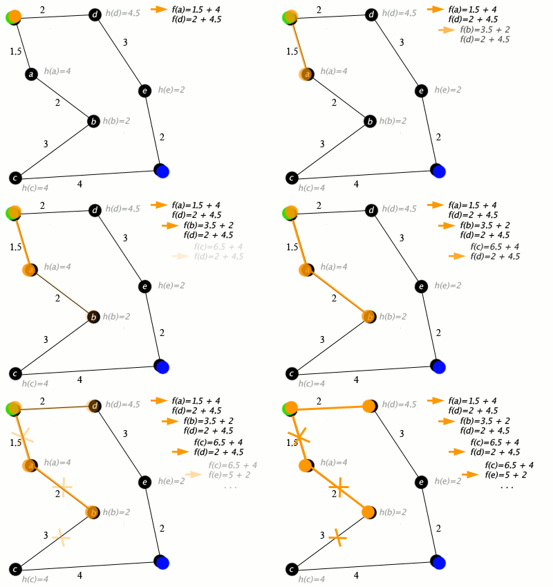 Key: green: start; blue: goal; orange: visited
The A* algorithm has real-world applications. In this example, edges are railroads and h(x) is the great-circle distance
The great-circle distance, orthodromic distance, or spherical distance is the distance between two points on a sphere, measured along the great-circle arc between them. This arc is the shortest path between the two points on the surface of the ...
(the shortest possible distance on a sphere) to the target. The algorithm is searching for a path between Washington, D.C., and Los Angeles.
Implementation details
There are a number of simple optimizations or implementation details that can significantly affect the performance of an A* implementation. The first detail to note is that the way the priority queue handles ties can have a significant effect on performance in some situations. If ties are broken so the queue behaves in a LIFO manner, A* will behave like depth-first search
Depth-first search (DFS) is an algorithm for traversing or searching tree or graph data structures. The algorithm starts at the root node (selecting some arbitrary node as the root node in the case of a graph) and explores as far as possible al ...
among equal cost paths (avoiding exploring more than one equally optimal solution).
When a path is required at the end of the search, it is common to keep with each node a reference to that node's parent. At the end of the search, these references can be used to recover the optimal path. If these references are being kept then it can be important that the same node doesn't appear in the priority queue more than once (each entry corresponding to a different path to the node, and each with a different cost). A standard approach here is to check if a node about to be added already appears in the priority queue. If it does, then the priority and parent pointers are changed to correspond to the lower-cost path. A standard binary heap
A binary heap is a heap (data structure), heap data structure that takes the form of a binary tree. Binary heaps are a common way of implementing priority queues. The binary heap was introduced by J. W. J. Williams in 1964 as a data structure fo ...
based priority queue does not directly support the operation of searching for one of its elements, but it can be augmented with a hash table
In computer science, a hash table is a data structure that implements an associative array, also called a dictionary or simply map; an associative array is an abstract data type that maps Unique key, keys to Value (computer science), values. ...
that maps elements to their position in the heap, allowing this decrease-priority operation to be performed in logarithmic time. Alternatively, a Fibonacci heap can perform the same decrease-priority operations in constant amortized time
In computer science, amortized analysis is a method for analyzing a given algorithm's complexity, or how much of a resource, especially time or memory, it takes to execute. The motivation for amortized analysis is that looking at the worst-case ...
.
Special cases
Dijkstra's algorithm
Dijkstra's algorithm ( ) is an algorithm for finding the shortest paths between nodes in a weighted graph, which may represent, for example, a road network. It was conceived by computer scientist Edsger W. Dijkstra in 1956 and published three ...
, as another example of a uniform-cost search algorithm, can be viewed as a special case of A* where for all ''x''... General depth-first search
Depth-first search (DFS) is an algorithm for traversing or searching tree or graph data structures. The algorithm starts at the root node (selecting some arbitrary node as the root node in the case of a graph) and explores as far as possible al ...
can be implemented using A* by considering that there is a global counter ''C'' initialized with a very large value. Every time we process a node we assign ''C'' to all of its newly discovered neighbors. After every single assignment, we decrease the counter ''C'' by one. Thus the earlier a node is discovered, the higher its value. Both Dijkstra's algorithm and depth-first search can be implemented more efficiently without including an value at each node.
Properties
Termination and completeness
On finite graphs with non-negative edge weights A* is guaranteed to terminate and is ''complete'', i.e. it will always find a solution (a path from start to goal) if one exists. On infinite graphs with a finite branching factor and edge costs that are bounded away from zero ( for some fixed ), A* is guaranteed to terminate only if there exists a solution.
Admissibility
A search algorithm is said to be ''admissible'' if it is guaranteed to return an optimal solution. If the heuristic function used by A* is admissible, then A* is admissible. An intuitive "proof" of this is as follows:
Call a node ''closed'' if it has been visited and is not in the open set. We ''close'' a node when we remove it from the open set. A basic property of the A* algorithm, which we'll sketch a proof of below, is that when is closed, is an optimistic estimate (lower bound) of the true distance from the start to the goal. So when the goal node, , is closed, is no more than the true distance. On the other hand, it is no less than the true distance, since it is the length of a path to the goal plus a heuristic term.
Now we'll see that whenever a node is closed, is an optimistic estimate. It is enough to see that whenever the open set is not empty, it has at least one node on an optimal path to the goal for which is the true distance from start, since in that case + underestimates the distance to goal, and therefore so does the smaller value chosen for the closed vertex. Let be an optimal path from the start to the goal. Let be the last closed node on for which is the true distance from the start to the goal (the start is one such vertex). The next node in has the correct value, since it was updated when was closed, and it is open since it is not closed.
Optimality and consistency
Algorithm A is optimally efficient with respect to a set of alternative algorithms Alts on a set of problems P if for every problem P in P and every algorithm A′ in Alts, the set of nodes expanded by A in solving P is a subset (possibly equal) of the set of nodes expanded by A′ in solving P. The definitive study of the optimal efficiency of A* is due to Rina Dechter and Judea Pearl.
They considered a variety of definitions of Alts and P in combination with A*'s heuristic being merely admissible or being both consistent
In deductive logic, a consistent theory is one that does not lead to a logical contradiction. A theory T is consistent if there is no formula \varphi such that both \varphi and its negation \lnot\varphi are elements of the set of consequences ...
and admissible. The most interesting positive result they proved is that A*, with a consistent heuristic, is optimally efficient with respect to all admissible A*-like search algorithms on all "non-pathological" search problems. Roughly speaking, their notion of the non-pathological problem is what we now mean by "up to tie-breaking". This result does not hold if A*'s heuristic is admissible but not consistent. In that case, Dechter and Pearl showed there exist admissible A*-like algorithms that can expand arbitrarily fewer nodes than A* on some non-pathological problems.
Optimal efficiency is about the ''set'' of nodes expanded, not the ''number'' of node expansions (the number of iterations of A*'s main loop). When the heuristic being used is admissible but not consistent, it is possible for a node to be expanded by A* many times, an exponential number of times in the worst case.
In such circumstances, Dijkstra's algorithm could outperform A* by a large margin. However, more recent research found that this pathological case only occurs in certain contrived situations where the edge weight of the search graph is exponential in the size of the graph and that certain inconsistent (but admissible) heuristics can lead to a reduced number of node expansions in A* searches.
Bounded relaxation
While the admissibility criterion guarantees an optimal solution path, it also means that A* must examine all equally meritorious paths to find the optimal path. To compute approximate shortest paths, it is possible to speed up the search at the expense of optimality by relaxing the admissibility criterion. Oftentimes we want to bound this relaxation, so that we can guarantee that the solution path is no worse than (1 + ''ε'') times the optimal solution path. This new guarantee is referred to as ''ε''-admissible.
There are a number of ''ε''-admissible algorithms:
*Weighted A*/Static Weighting's. If ''ha''(''n'') is an admissible heuristic function, in the weighted version of the A* search one uses , as the heuristic function, and perform the A* search as usual (which eventually happens faster than using ''ha'' since fewer nodes are expanded). The path hence found by the search algorithm can have a cost of at most ''ε'' times that of the least cost path in the graph.
*Convex Upward/Downward Parabola (XUP/XDP). Modification to the cost function in weighted A* to push optimality toward the start or goal. XDP gives paths which are near optimal close to the start, and XUP paths are near-optimal close to the goal. Both yield -optimal paths overall.
*: