quantitative genetics

Quantitative genetics deals with phenotypes that vary continuously (such as height or mass)—as opposed to discretely identifiable phenotypes and gene-products (such as eye-colour, or the presence of a particular biochemical).

Both branches use the frequencies of different alleles of a gene in breeding populations (gamodemes), and combine them with concepts from simple Mendelian inheritance to analyze inheritance patterns across generations and descendant lines. While population genetics can focus on particular genes and their subsequent metabolic products, quantitative genetics focuses more on the outward phenotypes, and makes only summaries of the underlying genetics.

Due to the continuous distribution of phenotypic values, quantitative genetics must employ many other statistical methods (such as the ''effect size'', the ''mean'' and the ''variance'') to link phenotypes (attributes) to genotypes. Some phenotypes may be analyzed either as discrete categories or as continuous phenotypes, depending on the definition of cut-off points, or on the ''metric'' used to quantify them. Mendel himself had to discuss this matter in his famous paper, especially with respect to his peas attribute ''tall/dwarf'', which actually was "length of stem". Analysis of quantitative trait loci, or QTL, is a more recent addition to quantitative genetics, linking it more directly to molecular genetics.

Gene effects

In diploid organisms, the average genotypic "value" (locus value) may be defined by the allele "effect" together with a dominance effect, and also by how genes interact with genes at other loci ( epistasis). The founder of quantitative genetics - Sir Ronald Fisher - perceived much of this when he proposed the first mathematics of this branch of genetics.

Being a statistician, he defined the gene effects as deviations from a central value—enabling the use of statistical concepts such as mean and variance, which use this idea. The central value he chose for the gene was the midpoint between the two opposing homo zygotes at the one locus. The deviation from there to the "greater" homozygous genotype can be named "''+a''" ; and therefore it is "''-a''" from that same midpoint to the "lesser" homozygote genotype. This is the "allele" effect mentioned above. The heterozygote deviation from the same midpoint can be named "''d''", this being the "dominance" effect referred to above. The diagram depicts the idea. However, in reality we measure phenotypes, and the figure also shows how observed phenotypes relate to the gene effects. Formal definitions of these effects recognize this phenotypic focus. Epistasis has been approached statistically as interaction (i.e., inconsistencies), but ''epigenetics'' suggests a new approach may be needed.

If 0a was known as "over-dominance".

Mendel's pea attribute "length of stem" provides us with a good example. Mendel stated that the tall true-breeding parents ranged from 6–7 feet in stem length (183 – 213 cm), giving a median of 198 cm (= P1). The short parents ranged from 0.75 to 1.25 feet in stem length (23 – 46 cm), with a rounded median of 34 cm (= P2). Their hybrid ranged from 6–7.5 feet in length (183–229 cm), with a median of 206 cm (= F1). The mean of P1 and P2 is 116 cm, this being the phenotypic value of the homozygotes midpoint (mp). The allele affect (''a'') is 1-mp= 82 cm = - 2-mp The dominance effect (''d'') is 1-mp= 90 cm. This historical example illustrates clearly how phenotype values and gene effects are linked.

Allele and genotype frequencies

To obtain means, variances and other statistics, both ''quantities'' and their ''occurrences'' are required. The gene effects (above) provide the framework for ''quantities'': and the ''frequencies'' of the contrasting alleles in the fertilization gamete-pool provide the information on ''occurrences''. Commonly, the frequency of the allele causing "more" in the phenotype (including dominance) is given the symbol ''p'', while the frequency of the contrasting allele is ''q''. An initial assumption made when establishing the algebra was that the parental population was infinite and random mating, which was made simply to facilitate the derivation. The subsequent mathematical development also implied that the frequency distribution within the effective gamete-pool was uniform: there were no local perturbations where ''p'' and ''q'' varied. Looking at the diagrammatic analysis of sexual reproduction, this is the same as declaring that ''p_P'' = ''p_g'' = ''p''; and similarly for ''q''. This mating system, dependent upon these assumptions, became known as "panmixia".

Panmixia rarely actually occurs in nature, as gamete distribution may be limited, for example by dispersal restrictions or by behaviour, or by chance sampling (those local perturbations mentioned above). It is well known that there is a huge wastage of gametes in Nature, which is why the diagram depicts a ''potential'' gamete-pool separately to the ''actual'' gamete-pool. Only the latter sets the definitive frequencies for the zygotes: this is the true "gamodeme" ("gamo" refers to the gametes, and "deme" derives from Greek for "population"). But, under Fisher's assumptions, the ''gamodeme'' can be effectively extended back to the ''potential'' gamete-pool, and even back to the parental base-population (the "source" population). The random sampling arising when small "actual" gamete-pools are sampled from a large "potential" gamete-pool is known as '' genetic drift'', and is considered subsequently.

While panmixia may not be widely extant, the ''potential'' for it does occur, although it may be only ephemeral because of those local perturbations. It has been shown, for example, that the F2 derived from ''random fertilization of F1 individuals'' (an ''allogamous'' F2), following hybridization, is an ''origin'' of a new ''potentially'' panmictic population. It has also been shown that if panmictic random fertilization occurred continually, it would maintain the same allele and genotype frequencies across each successive panmictic sexual generation—this being the ''Hardy Weinberg'' equilibrium. However, as soon as genetic drift was initiated by local random sampling of gametes, the equilibrium would cease.

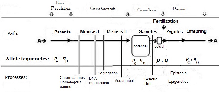
Random fertilization

Male and female gametes within the actual fertilizing pool are considered usually to have the same frequencies for their corresponding alleles. (Exceptions have been considered.) This means that when ''p'' male gametes carrying the ''A'' allele randomly fertilize ''p'' female gametes carrying that same allele, the resulting zygote has genotype ''AA'', and, under random fertilization, the combination occurs with a frequency of ''p'' x ''p'' (= ''p²''). Similarly, the zygote ''aa'' occurs with a frequency of ''q²''. Heterozygotes (''Aa'') can arise in two ways: when ''p'' male (''A'' allele) randomly fertilize ''q'' female (''a'' allele) gametes, and ''vice versa''. The resulting frequency for the heterozygous zygotes is thus ''2pq''. Notice that such a population is never more than half heterozygous, this maximum occurring when p=q= 0.5.

In summary then, under random fertilization, the zygote (genotype) frequencies are the quadratic expansion of the gametic (allelic) frequencies: $(p+q)^2 = p^2 + 2pq + q^2 = 1$. (The "=1" states that the frequencies are in fraction form, not percentages; and that there are no omissions within the framework proposed.)

Notice that "random fertilization" and "panmixia" are ''not'' synonyms.

Mendel's research cross – a contrast

Mendel's pea experiments were constructed by establishing true-breeding parents with "opposite" phenotypes for each attribute. This meant that each opposite parent was homozygous for its respective allele only. In our example, "tall ''vs'' dwarf", the tall parent would be genotype ''TT'' with ''p'' = 1 (and ''q'' = 0); while the dwarf parent would be genotype ''tt'' with ''q'' = 1 (and ''p'' = 0). After controlled crossing, their hybrid is ''Tt'', with ''p'' = ''q'' = ½. However, the frequency of this heterozygote = 1, because this is the F1 of an artificial cross: it has not arisen through random fertilization. The F2 generation was produced by natural self-pollination of the F1 (with monitoring against insect contamination), resulting in ''p'' = ''q'' = ½ being maintained. Such an F2 is said to be "autogamous". However, the genotype frequencies (0.25 ''TT'', 0.5 ''Tt'', 0.25 ''tt'') have arisen through a mating system very different from random fertilization, and therefore the use of the quadratic expansion has been avoided. The numerical values obtained were the same as those for random fertilization only because this is the special case of having originally crossed homozygous opposite parents. We can notice that, because of the dominance of ''T-'' requency (0.25 + 0.5)over ''tt'' requency 0.25 the 3:1 ratio is still obtained.

A cross such as Mendel's, where true-breeding (largely homozygous) opposite parents are crossed in a controlled way to produce an F1, is a special case of hybrid structure. The F1 is often regarded as "entirely heterozygous" for the gene under consideration. However, this is an over-simplification and does not apply generally—for example when individual parents are not homozygous, or when ''populations'' inter-hybridise to form ''hybrid swarms''. The general properties of intra-species hybrids (F1) and F2 (both "autogamous" and "allogamous") are considered in a later section.

Self fertilization – an alternative

Having noticed that the pea is naturally self-pollinated, we cannot continue to use it as an example for illustrating random fertilization properties. Self-fertilization ("selfing") is a major alternative to random fertilization, especially within Plants. Most of the Earth's cereals are naturally self-pollinated (rice, wheat, barley, for example), as well as the pulses. Considering the millions of individuals of each of these on Earth at any time, it's obvious that self-fertilization is at least as significant as random fertilization. Self-fertilization is the most intensive form of ''inbreeding'', which arises whenever there is restricted independence in the genetical origins of gametes. Such reduction in independence arises if parents are already related, and/or from genetic drift or other spatial restrictions on gamete dispersal. Path analysis demonstrates that these are tantamount to the same thing. Arising from this background, the ''inbreeding coefficient'' (often symbolized as F or ''f'') quantifies the effect of inbreeding from whatever cause. There are several formal definitions of ''f'', and some of these are considered in later sections. For the present, note that for a long-term self-fertilized species ''f'' = 1.
Natural self-fertilized populations are not single " ''pure lines'' ", however, but mixtures of such lines. This becomes particularly obvious when considering more than one gene at a time. Therefore, allele frequencies (''p'' and ''q'') other than 1 or 0 are still relevant in these cases (refer back to the Mendel Cross section). The genotype frequencies take a different form, however.

In general, the genotype frequencies become $$^2(1-f)+pf/math> for AA and $2pq(1-f)$ for Aa and $$^2(1-f)+qf/math> for aa.

Notice that the frequency of the heterozygote declines in proportion to ''f''. When ''f'' = 1, these three frequencies become respectively p, 0 and q Conversely, when f = 0, they reduce to the random-fertilization quadratic expansion shown previously.

Population mean

The population mean shifts the central reference point from the homozygote midpoint (mp) to the mean of a sexually reproduced population. This is important not only to relocate the focus into the natural world, but also to use a measure of ''central tendency'' used by Statistics/Biometrics. In particular, the square of this mean is the Correction Factor, which is used to obtain the genotypic variances later.

For each genotype in turn, its allele effect is multiplied by its genotype frequency; and the products are accumulated across all genotypes in the model. Some algebraic simplification usually follows to reach a succinct result.

The mean after random fertilization

The contribution of AA is $p^2 (+)a$, that of Aa is $2pq d$, and that of aa is $q^2 (-)a$. Gathering together the two a terms and accumulating over all, the result is: $a(p^2-q^2) + 2pq d$. Simplification is achieved by noting that $(p^2-q^2) = (p-q)(p+q)$, and by recalling that $(p+q) = 1$, thereby reducing the right-hand term to $(p-q)$.

The succinct result is therefore $G = a(p-q) + 2pqd$.

This defines the population mean as an "offset" from the homozygote midpoint (recall a and d are defined as ''deviations'' from that midpoint). The Figure depicts G across all values of p for several values of d, including one case of slight over-dominance. Notice that G is often negative, thereby emphasizing that it is itself a ''deviation'' (from mp).

Finally, to obtain the ''actual'' Population Mean in "phenotypic space", the midpoint value is added to this offset: $P = G + mp$.

An example arises from data on ear length in maize. Assuming for now that one gene only is represented, a = 5.45 cm, d = 0.12 cm irtually "0", really mp = 12.05 cm. Further assuming that p = 0.6 and q = 0.4 in this example population, then:

G = 5.45 (0.6 − 0.4) + (0.48)0.12 = 1.15 cm (rounded); and

P = 1.15 + 12.05 = 13.20 cm (rounded).

The mean after long-term self-fertilization

The contribution of AA is $p (+a)$, while that of aa is $q (-a)$. ee above for the frequencies.Gathering these two a terms together leads to an immediately very simple final result:

$G_ = a(p-q)$. As before, $P = G + mp$.

Often, "G_(f=1)" is abbreviated to "G₁".

Mendel's peas can provide us with the allele effects and midpoint (see previously); and a mixed self-pollinated population with p = 0.6 and q = 0.4 provides example frequencies. Thus:

G_(f=1) = 82 (0.6 − .04) = 59.6 cm (rounded); and

P_(f=1) = 59.6 + 116 = 175.6 cm (rounded).

The mean – generalized fertilization

A general formula incorporates the inbreeding coefficient ''f'', and can then accommodate any situation. The procedure is exactly the same as before, using the weighted genotype frequencies given earlier. After translation into our symbols, and further rearrangement:

\begin
G_ & = a (q-p) + pqd-f(2pqd)\\
& = a(p-q) + (1-f) 2pqd \\
& = G_ - f\ 2pqd
\end
Here, G₀ is G, which was given earlier. (Often, when dealing with inbreeding, "G₀" is preferred to "G".)

Supposing that the maize example iven earlierhad been constrained on a holme (a narrow riparian meadow), and had partial inbreeding to the extent of ''f ''= 0.25, then, using the third version (above) of G_f:

G_''0.25'' = 1.15 − 0.25 (0.48) 0.12 = 1.136   cm (rounded), with P_0.25 = 13.194   cm (rounded).

There is hardly any effect from inbreeding in this example, which arises because there was virtually no dominance in this attribute (d → 0). Examination of all three versions of G_''f'' reveals that this would lead to trivial change in the Population mean. Where dominance was notable, however, there would be considerable change.

Genetic drift

Genetic drift was introduced when discussing the likelihood of panmixia being widely extant as a natural fertilization pattern. ee section on Allele and Genotype frequencies.Here the sampling of gametes from the ''potential'' gamodeme is discussed in more detail. The sampling involves random fertilization between pairs of random gametes, each of which may contain either an A or an a allele. The sampling is therefore binomial sampling. Each sampling "packet" involves 2N alleles, and produces N zygotes (a "progeny" or a "line") as a result. During the course of the reproductive period, this sampling is repeated over and over, so that the final result is a mixture of sample progenies. The result is ''dispersed random fertilization'' $\left( \bigodot \right)$ These events, and the overall end-result, are examined here with an illustrative example.

The "base" allele frequencies of the example are those of the ''potential gamodeme'': the frequency of A is p_g = 0.75, while the frequency of a is q_g = 0.25. 'White label'' "1" in the diagram.Five example actual gamodemes are binomially sampled out of this base (s = the number of samples = 5), and each sample is designated with an "index" k: with k = 1 .... s sequentially. (These are the sampling "packets" referred to in the previous paragraph.) The number of gametes involved in fertilization varies from sample to sample, and is given as 2N_k t ''white label'' "2" in the diagram The total (Σ) number of gametes sampled overall is 52 'white label'' "3" in the diagram Because each sample has its own size, ''weights'' are needed to obtain averages (and other statistics) when obtaining the overall results. These are $\omega_k = 2N_k / (\sum_^s 2N_k)$, and are given at ''white label'' "4" in the diagram.

The sample gamodemes – genetic drift

Following completion of these five binomial sampling events, the resultant actual gamodemes each contained different allele frequencies—(p_k and q_k). hese are given at ''white label'' "5" in the diagram.This outcome is actually the genetic drift itself. Notice that two samples (k = 1 and 5) happen to have the same frequencies as the ''base'' (''potential'') gamodeme. Another (k = 3) happens to have the ''p'' and ''q'' "reversed". Sample (k = 2) happens to be an "extreme" case, with p_k = 0.9 and q_k = 0.1 ; while the remaining sample (k = 4) is "middle of the range" in its allele frequencies. All of these results have arisen only by "chance", through binomial sampling. Having occurred, however, they set in place all the downstream properties of the progenies.

Because sampling involves chance, the ''probabilities'' ( _k ) of obtaining each of these samples become of interest. These binomial probabilities depend on the starting frequencies (p_g and q_g) and the sample size (2N_k). They are tedious to obtain, but are of considerable interest. ee ''white label'' "6" in the diagram.The two samples (k = 1, 5), with the allele frequencies the same as in the ''potential gamodeme'', had higher "chances" of occurring than the other samples. Their binomial probabilities did differ, however, because of their different sample sizes (2N_k). The "reversal" sample (k = 3) had a very low Probability of occurring, confirming perhaps what might be expected. The "extreme" allele frequency gamodeme (k = 2) was not "rare", however; and the "middle of the range" sample (k=4) ''was'' rare. These same Probabilities apply also to the progeny of these fertilizations.

Here, some ''summarizing'' can begin. The ''overall allele frequencies'' in the progenies bulk are supplied by weighted averages of the appropriate frequencies of the individual samples. That is: $p_ = \sum_^s \omega_ \ p_$ and $q_ = \sum_^s \omega_ \ q_$. (Notice that k is replaced by • for the overall result—a common practice.) The results for the example are p_• = 0.631 and q_• = 0.369 'black label'' "5" in the diagram These values are quite different to the starting ones (p_g and q_g) 'white label'' "1" The sample allele frequencies also have variance as well as an average. This has been obtained using the ''sum of squares (SS)'' method ee to the right of ''black label'' "5" in the diagram urther discussion on this variance occurs in the section below on Extensive genetic drift.

The progeny lines – dispersion

The ''genotype frequencies'' of the five sample progenies are obtained from the usual quadratic expansion of their respective allele frequencies (''random fertilization''). The results are given at the diagram's ''white label'' "7" for the homozygotes, and at ''white label'' "8" for the heterozygotes. Re-arrangement in this manner prepares the way for monitoring inbreeding levels. This can be done either by examining the level of ''total'' homozygosis p²_k + q²_k) = (1 − 2p_kq_k), or by examining the level of heterozygosis (2p_kq_k), as they are complementary. Notice that samples ''k= 1, 3, 5'' all had the same level of heterozygosis, despite one being the "mirror image" of the others with respect to allele frequencies. The "extreme" allele-frequency case (k= ''2'') had the most homozygosis (least heterozygosis) of any sample. The "middle of the range" case (k= ''4'') had the least homozygosity (most heterozygosity): they were each equal at 0.50, in fact.

The ''overall summary'' can continue by obtaining the ''weighted average'' of the respective genotype frequencies for the progeny bulk. Thus, for AA, it is $p^2_\centerdot = \sum_k^s \omega_k \ p_k^2$, for Aa , it is $2p_\centerdot q_\centerdot = \sum_k^s \omega_k \ 2 p_k q_k$ and for aa, it is $q_\centerdot^2 = \sum_k^s \omega_k \ q_k^2$. The example results are given at ''black label'' "7" for the homozygotes, and at ''black label'' "8" for the heterozygote. Note that the heterozygosity mean is ''0.3588'', which the next section uses to examine inbreeding resulting from this genetic drift.

The next focus of interest is the dispersion itself, which refers to the "spreading apart" of the progenies' ''population means''. These are obtained as $G_k = a (p_k - q_k) + 2p_k q_k d$ ee section on the Population mean for each sample progeny in turn, using the example gene effects given at ''white label'' "9" in the diagram. Then, each $P_k = G_k + mp$ is obtained also t ''white label'' "10" in the diagram Notice that the "best" line (k = 2) had the ''highest'' allele frequency for the "more" allele (A) (it also had the highest level of homozygosity). The ''worst'' progeny (k = 3) had the highest frequency for the "less" allele (a), which accounted for its poor performance. This "poor" line was less homozygous than the "best" line; and it shared the same level of homozygosity, in fact, as the two ''second-best'' lines (k = 1, 5). The progeny line with both the "more" and the "less" alleles present in equal frequency (k = 4) had a mean below the ''overall average'' (see next paragraph), and had the lowest level of homozygosity. These results reveal the fact that the alleles most prevalent in the "gene-pool" (also called the "germplasm") determine performance, not the level of homozygosity per se. Binomial sampling alone effects this dispersion.

The ''overall summary'' can now be concluded by obtaining $G_ = \sum_k^s \omega_k \ G_k$ and $P_ = \sum_k^s \omega_k \ P_k$. The example result for P_• is 36.94 (''black label'' "10" in the diagram). This later is used to quantify ''inbreeding depression'' overall, from the gamete sampling. ee the next section.However, recall that some "non-depressed" progeny means have been identified already (k = 1, 2, 5). This is an enigma of inbreeding—while there may be "depression" overall, there are usually superior lines among the gamodeme samplings.

The equivalent post-dispersion panmictic – inbreeding

Included in the ''overall summary'' were the average allele frequencies in the mixture of progeny lines (p_• and q_•). These can now be used to construct a hypothetical panmictic equivalent. This can be regarded as a "reference" to assess the changes wrought by the gamete sampling. The example appends such a panmictic to the right of the Diagram. The frequency of AA is therefore (p_•)² = 0.3979. This is less than that found in the dispersed bulk (0.4513 at ''black label'' "7"). Similarly, for aa, (q_•)² = 0.1303—again less than the equivalent in the progenies bulk (0.1898). Clearly, ''genetic drift'' has increased the overall level of homozygosis by the amount (0.6411 − 0.5342) = 0.1069. In a complementary approach, the heterozygosity could be used instead. The panmictic equivalent for Aa is 2 p_• q_• = 0.4658, which is ''higher'' than that in the sampled bulk (0.3588) 'black label'' "8" The sampling has caused the heterozygosity to decrease by 0.1070, which differs trivially from the earlier estimate because of rounding errors.

The inbreeding coefficient (''f'') was introduced in the early section on Self Fertilization. Here, a formal definition of it is considered: ''f'' is the probability that two "same" alleles (that is A and A, or a and a), which fertilize together are of common ancestral origin—or (more formally) ''f'' is the probability that two homologous alleles are autozygous. Consider any random gamete in the ''potential'' gamodeme that has its syngamy partner restricted by binomial sampling. The probability that that second gamete is homologous autozygous to the first is 1/(2N), the reciprocal of the gamodeme size. For the five example progenies, these quantities are 0.1, 0.0833, 0.1, 0.0833 and 0.125 respectively, and their weighted average is 0.0961. This is the ''inbreeding coefficient'' of the example progenies bulk, provided it is ''unbiased'' with respect to the full binomial distribution. An example based upon ''s = 5'' is likely to be biased, however, when compared to an appropriate entire binomial distribution based upon the sample number (''s'') approaching infinity (''s → ∞''). Another derived definition of ''f'' for the full Distribution is that ''f'' also equals the rise in homozygosity, which equals the fall in heterozygosity. For the example, these frequency changes are ''0.1069'' and ''0.1070'', respectively. This result is different to the above, indicating that bias with respect to the full underlying distribution is present in the example. For the example ''itself'', these latter values are the better ones to use, namely ''f_•'' = 0.10695.

The ''population mean'' of the equivalent panmictic is found as '' (p_•-q_•) + 2 p_•q_• d+ mp''. Using the example ''gene effects'' (''white label'' "9" in the diagram), this mean is $P_ =$ 37.87. The equivalent mean in the dispersed bulk is 36.94 (''black label'' "10"), which is depressed by the amount ''0.93''. This is the ''inbreeding depression'' from this Genetic Drift. However, as noted previously, three progenies were ''not'' depressed (k = 1, 2, 5), and had means even greater than that of the panmictic equivalent. These are the lines a plant breeder looks for in a line selection programme.

Extensive binomial sampling – is panmixia restored?

If the number of binomial samples is large (s → ∞ ), then p_• → p_g and q_• → q_g. It might be queried whether panmixia would effectively re-appear under these circumstances. However, the sampling of allele frequencies has ''still occurred'', with the result that σ²_{p, q} ≠ 0.This is read as "σ ²_p and/or σ ²_q". As ''p'' and ''q'' are complementary, σ ²_p ≡ σ ²_q and σ ²_p = σ ²_q. In fact, as s → ∞, the $\sigma^2_ \to \tfrac$, which is the ''variance'' of the ''whole binomial distribution''. Furthermore, the "Wahlund equations" show that the progeny-bulk ''homozygote'' frequencies can be obtained as the sums of their respective average values (p²_• or q²_•) ''plus'' σ²_{p, q}. Likewise, the bulk ''heterozygote'' frequency is (2 p_• q_•) ''minus'' twice the σ²_{p, q}. The variance arising from the binomial sampling is conspicuously present. Thus, even when s → ∞, the progeny-bulk ''genotype'' frequencies still reveal ''increased homozygosis'', and ''decreased heterozygosis'', there is still ''dispersion of progeny means'', and still ''inbreeding'' and ''inbreeding depression''. That is, panmixia is ''not'' re-attained once lost because of genetic drift (binomial sampling). However, a new ''potential'' panmixia can be initiated via an allogamous F2 following hybridization.

Continued genetic drift – increased dispersion and inbreeding

Previous discussion on genetic drift examined just one cycle (generation) of the process. When the sampling continues over successive generations, conspicuous changes occur in σ²_{p, q} and ''f''. Furthermore, another "index" is needed to keep track of "time": t = 1 .... y where y = the number of "years" (generations) considered. The methodology often is to add the current binomial increment (Δ = "''de novo''") to what has occurred previously. The entire Binomial Distribution is examined here. here is no further benefit to be had from an abbreviated example.

= Dispersion via σ²_p,q

=
Earlier this variance (σ ²_p,q) was seen to be:-
$\begin \sigma ^2_ & = p_g q_g \ / \ 2N \\ & = p_g q_g \left( \frac \right) \\ & = p_g q_g \ f \\ & = p_g q_g \ \Delta f \ \scriptstyle \text \end$

With the extension over time, this is also the result of the ''first'' cycle, and so is $\sigma^2_1$ (for brevity). At cycle 2, this variance is generated yet again—this time becoming the ''de novo'' variance ($\Delta \sigma^2$)—and accumulates to what was present already—the "carry-over" variance. The ''second'' cycle variance ($\sigma^2_2$) is the weighted sum of these two components, the weights being $1$ for the ''de novo'' and $\left( 1 - \tfrac \right)$ = $\left( 1 - \Delta f \right)$ for the"carry-over".
Thus,

The extension to generalize to any time ''t'' , after considerable simplification, becomes:-

Because it was this variation in allele frequencies that caused the "spreading apart" of the progenies' means (''dispersion''), the change in σ²_t over the generations indicates the change in the level of the ''dispersion''.

=Dispersion via ''f''

=
The method for examining the inbreeding coefficient is similar to that used for ''σ ²_p,q''. The same weights as before are used respectively for ''de novo f'' ( Δ f ) ecall this is 1/(2N) and ''carry-over f''. Therefore, $f_2 = \left( 1 \right) \Delta f + \left( 1 - \Delta f \right) f_1$ , which is similar to Equation (1) in the previous sub-section.

In general, after rearrangement, $\begin f_t & = \Delta f + \left( 1 - \Delta f \right) f_ \\ & = \Delta f \left( 1 - f_ \right) + f_ \end$ The graphs to the left show levels of inbreeding over twenty generations arising from genetic drift for various ''actual gamodeme'' sizes (2N).

Still further rearrangements of this general equation reveal some interesting relationships.

(A) After some simplification, $\left( f_t - f_ \right) = \Delta f \left( 1 - f_ \right) = \delta f_t$. The left-hand side is the difference between the current and previous levels of inbreeding: the ''change in inbreeding'' (δf_t). Notice, that this ''change in inbreeding'' (δf_t) is equal to the ''de novo inbreeding'' (Δf) only for the first cycle—when f_t-1 is ''zero''.

(B) An item of note is the (1-f_t-1), which is an "index of ''non-inbreeding''". It is known as the ''panmictic index''. $P_ = \left( 1 - f_ \right)$.

(C) Further useful relationships emerge involving the ''panmictic index''.
$\begin \Delta f & = \frac \\ & = 1 - \frac \end$.
(D) A key link emerges between ''σ ²_p,q'' and ''f''. Firstly...
$\begin f_t & = 1 - \left( 1 -1 \Delta f \right) ^t \left( 1 - f_0 \right) \end$
Secondly, presuming that f₀ = 0, the right-hand side of this equation reduces to the section within the brackets of Equation (2) at the end of the last sub-section. That is, if initially there is no inbreeding, $\sigma^2_t = p_g q_g f_t$ ! Furthermore, if this then is rearranged, $f_t = \tfrac$. That is, when initial inbreeding is zero, the two principal viewpoints of ''binomial gamete sampling'' (genetic drift) are directly inter-convertible.

Selfing within random fertilization

It is easy to overlook that ''random fertilization'' includes self-fertilization. Sewall Wright showed that a proportion 1/N of ''random fertilizations'' is actually ''self fertilization'' $\left( \bigotimes \right)$, with the remainder (N-1)/N being ''cross fertilization'' $\left( \mathsf \right)$. Following path analysis and simplification, the new view ''random fertilization inbreeding'' was found to be: $f_t = \Delta f \left( 1 + f_ \right) + \tfrac f_$. Upon further rearrangement, the earlier results from the binomial sampling were confirmed, along with some new arrangements. Two of these were potentially very useful, namely: (A) f_t = \Delta f \left 1 + f_ \left( 2N-1 \right) \right; and (B) $f_t = \Delta f \left( 1 - f_ \right) + f_$.

The recognition that selfing may ''intrinsically be a part of'' random fertilization leads to some issues about the use of the previous ''random fertilization'' 'inbreeding coefficient'. Clearly, then, it is inappropriate for any species incapable of ''self fertilization'', which includes plants with self-incompatibility mechanisms, dioecious plants, and bisexual animals. The equation of Wright was modified later to provide a version of random fertilization that involved only ''cross fertilization'' with no ''self fertilization''. The proportion 1/N formerly due to ''selfing'' now defined the ''carry-over'' gene-drift inbreeding arising from the previous cycle. The new version is:
$f_ = f_ + \Delta f \left( 1 + f_ - 2 f_ \right)$.

The graphs to the right depict the differences between standard ''random fertilization'' RF, and random fertilization adjusted for "cross fertilization alone" CF. As can be seen, the issue is non-trivial for small gamodeme sample sizes.

It now is necessary to note that not only is "panmixia" ''not'' a synonym for "random fertilization", but also that "random fertilization" is ''not'' a synonym for "cross fertilization".

Homozygosity and heterozygosity

In the sub-section on "The sample gamodemes – Genetic drift", a series of gamete samplings was followed, an outcome of which was an increase in homozygosity at the expense of heterozygosity. From this viewpoint, the rise in homozygosity was due to the gamete samplings. Levels of homozygosity can be viewed also according to whether homozygotes arose allozygously or autozygously. Recall that autozygous alleles have the same allelic origin, the likelihood (frequency) of which ''is'' the inbreeding coefficient (''f'') by definition. The proportion arising ''allozygously'' is therefore (1-f). For the A-bearing gametes, which are present with a general frequency of p, the overall frequency of those that are autozygous is therefore (f ''p''). Similarly, for a-bearing gametes, the autozygous frequency is (f ''q''). These two viewpoints regarding genotype frequencies must be connected to establish consistency.

Following firstly the ''auto/allo'' viewpoint, consider the ''allozygous'' component. This occurs with the frequency of (1-f), and the alleles unite according to the ''random fertilization'' quadratic expansion. Thus:
\left( 1-f \right) \left p_0 + q_0 \right^2 = \left( 1-f \right) \left p_0^2 + q_0^2 \right+ \left( 1-f \right) \left 2 p_0 q_0 \right Consider next the ''autozygous'' component. As these alleles are ''autozygous'', they are effectively selfings, and produce either AA or aa genotypes, but no heterozygotes. They therefore produce $f p_0$ ''"AA"'' homozygotes plus $f q_0$ ''"aa"'' homozygotes. Adding these two components together results in:
\left \left( 1-f \right) p_0^2 + f p_0 \right for the AA homozygote; \left \left( 1-f \right) q_0^2 + f q_0 \right for the aa homozygote; and $\left( 1-f \right) 2 p_0 q_0$ for the Aa heterozygote. This is the same equation as that presented earlier in the section on "Self fertilization – an alternative". The reason for the decline in heterozygosity is made clear here. Heterozygotes can arise ''only'' from the allozygous component, and its frequency in the sample bulk is just (1-f): hence this must also be the factor controlling the frequency of the heterozygotes.

Secondly, the ''sampling'' viewpoint is re-examined. Previously, it was noted that the decline in heterozygotes was $f \left( 2 p_0 q_0 \right)$. This decline is distributed equally towards each homozygote; and is added to their basic ''random fertilization'' expectations. Therefore, the genotype frequencies are: $\left( p_0^2 + f p_0 q_0 \right)$ for the ''"AA"'' homozygote; $\left( q_0^2 + f p_0 q_0 \right)$ for the ''"aa"'' homozygote; and $2 p_0 q_0 - f \left( 2 p_0 q_0 \right)$ for the heterozygote.

Thirdly, the ''consistency'' between the two previous viewpoints needs establishing. It is apparent at once rom the corresponding equations abovethat the heterozygote frequency is the same in both viewpoints. However, such a straightforward result is not immediately apparent for the homozygotes. Begin by considering the AA homozygote's final equation in the ''auto/allo'' paragraph above:- \left \left( 1-f \right) p_0^2 + f p_0 \right. Expand the brackets, and follow by re-gathering ithin the resultantthe two new terms with the common-factor ''f'' in them. The result is: $p_0^2 - f \left( p_0^2 - p_0 \right)$. Next, for the parenthesized " ''p²₀'' ", a ''(1-q)'' is substituted for a ''p'', the result becoming p_0^2 - f \left p_0 \left( 1-q_0 \right) - p_0 \right. Following that substitution, it is a straightforward matter of multiplying-out, simplifying and watching signs. The end result is $p_0^2 + f p_0 q_0$, which is exactly the result for AA in the ''sampling'' paragraph. The two viewpoints are therefore ''consistent'' for the AA homozygote. In a like manner, the consistency of the aa viewpoints can also be shown. The two viewpoints are consistent for all classes of genotypes.

Extended principles

Other fertilization patterns

In previous sections, dispersive random fertilization (''genetic drift'') has been considered comprehensively, and self-fertilization and hybridizing have been examined to varying degrees. The diagram to the left depicts the first two of these, along with another "spatially based" pattern: ''islands''. This is a pattern of ''random fertilization'' featuring ''dispersed gamodemes'', with the addition of "overlaps" in which ''non-dispersive'' random fertilization occurs. With the ''islands'' pattern, individual gamodeme sizes (2N) are observable, and overlaps (m) are minimal. This is one of Sewall Wright's array of possibilities. In addition to "spatially" based patterns of fertilization, there are others based on either "phenotypic" or "relationship" criteria. The ''phenotypic'' bases include ''assortative'' fertilization (between similar phenotypes) and ''disassortative'' fertilization (between opposite phenotypes). The ''relationship'' patterns include ''sib crossing'', ''cousin crossing'' and ''backcrossing''—and are considered in a separate section. ''Self fertilization'' may be considered both from a spatial or relationship point of view.

"Islands" random fertilization

The breeding population consists of s small dispersed random fertilization gamodemes of sample size $2N_k$ ( k = 1 ... ''s'' ) with " ''overlaps'' " of proportion $m_k$ in which non-dispersive random fertilization occurs. The '' dispersive proportion '' is thus $\left( 1 - m_k \right)$. The bulk population consists of ''weighted averages'' of sample sizes, allele and genotype frequencies and progeny means, as was done for genetic drift in an earlier section. However, each ''gamete sample size'' is reduced to allow for the ''overlaps'', thus finding a $2 N_k$ effective for $\left( 1 - m_k \right)$.

For brevity, the argument is followed further with the subscripts omitted. Recall that $\tfrac$ is $\Delta f$ in general. ere, and following, the ''2N'' refers to the ''previously defined'' sample size, not to any "islands adjusted" version.
After simplification, $^ \Delta f = \frac$
Notice that when ''m = 0'' this reduces to the previous ''Δ f''. The reciprocal of this furnishes an estimate of the " $2 N_k$ ''effective for $\left( 1 - m_k \right)$'' ", mentioned above.

This Δf is also substituted into the previous ''inbreeding coefficient'' to obtain
$= \ + \left( 1 - \ \right) \$ where ''t'' is the index over generations, as before.

The effective ''overlap proportion'' can be obtained also, as
m_t = 1 - \left \frac \right^

The graphs to the right show the ''inbreeding'' for a gamodeme size of ''2N = 50'' for ''ordinary dispersed random fertilization '' (RF) ''(m=0)'', and for ''four overlap levels ( m = 0.0625, 0.125, 0.25, 0.5 )'' of islands ''random fertilization''. There has indeed been reduction in the inbreeding resulting from the ''non-dispersed random fertilization'' in the overlaps. It is particularly notable as m → 0.50. Sewall Wright suggested that this value should be the limit for the use of this approach.

Allele shuffling – allele substitution

The ''gene-model'' examines the heredity pathway from the point of view of "inputs" (alleles/gametes) and "outputs" (genotypes/zygotes), with fertilization being the "process" converting one to the other. An alternative viewpoint concentrates on the "process" itself, and considers the zygote genotypes as arising from allele shuffling. In particular, it regards the results as if one allele had "substituted" for the other during the shuffle, together with a residual that deviates from this view. This formed an integral part of Fisher's method, in addition to his use of frequencies and effects to generate his genetical statistics. A discursive derivation of the ''allele substitution'' alternative follows.

Suppose that the usual random fertilization of gametes in a "base" gamodeme—consisting of ''p'' gametes (A) and ''q'' gametes (a)—is replaced by fertilization with a "flood" of gametes all containing a single allele (A or a, but not both). The zygotic results can be interpreted in terms of the "flood" allele having "substituted for" the alternative allele in the underlying "base" gamodeme. The diagram assists in following this viewpoint: the upper part pictures an A substitution, while the lower part shows an a substitution. (The diagram's "RF allele" is the allele in the "base" gamodeme.)

Consider the upper part firstly. Because ''base'' A is present with a frequency of ''p'', the ''substitute'' A fertilizes it with a frequency of ''p'' resulting in a zygote AA with an allele effect of ''a''. Its contribution to the outcome, therefore, is the product $\left( p \ a \right)$. Similarly, when the ''substitute'' fertilizes ''base'' a (resulting in Aa with a frequency of ''q'' and heterozygote effect of ''d''), the contribution is $\left( q \ d \right)$. The overall result of substitution by A is, therefore, $\left( p \ a + q \ d \right)$. This is now oriented towards the population mean ee earlier sectionby expressing it as a deviate from that mean : $\left( p \ a + q \ d \right) - G$

After some algebraic simplification, this becomes \beta _A = q \ \left + \left( q - p \right) d \right
- the ''substitution effect'' of A.

A parallel reasoning can be applied to the lower part of the diagram, taking care with the differences in frequencies and gene effects. The result is the ''substitution effect'' of a, which is \beta _a = - \ p \left a + \left( q -p \right) d \right
The common factor inside the brackets is the ''average allele substitution effect'', and is $\beta = a + \left( q - p \right) d$
It can also be derived in a more direct way, but the result is the same.

In subsequent sections, these substitution effects help define the gene-model genotypes as consisting of a partition predicted by these new effects (substitution ''expectations''), and a residual (substitution deviations) between these expectations and the previous gene-model effects. The ''expectations'' are also called the breeding values and the deviations are also called dominance deviations.

Ultimately, the variance arising from the ''substitution expectations'' becomes the so-called ''Additive genetic variance (σ²_A)'' (also the ''Genic variance'' )— while that arising from the ''substitution deviations'' becomes the so-called ''Dominance variance (σ²_D)''. It is noticeable that neither of these terms reflects the true meanings of these variances. The "genic variance" is less dubious than the '' additive genetic variance'', and more in line with Fisher's own name for this partition. A less-misleading name for the ''dominance deviations variance'' is the "quasi-dominance variance" ee following sections for further discussion These latter terms are preferred herein.

Gene effects redefined

The gene-model effects (a, d and -a) are important soon in the derivation of the ''deviations from substitution'', which were first discussed in the previous ''Allele Substitution'' section. However, they need to be redefined themselves before they become useful in that exercise. They firstly need to be re-centralized around the population mean (G), and secondly they need to be re-arranged as functions of β, the ''average allele substitution effect''.

Consider firstly the re-centralization. The re-centralized effect for AA is a• = a - G which, after simplification, becomes a• = 2''q''(a-''p''d). The similar effect for Aa is d• = d - G = a(''q''-''p'') + d(1-2''pq''), after simplification. Finally, the re-centralized effect for aa is (-a)• = -2''p''(a+''q''d).

Secondly, consider the re-arrangement of these re-centralized effects as functions of β. Recalling from the "Allele Substitution" section that β = +(q-p)d rearrangement gives a = � -(q-p)d''. After substituting this for a in a• and simplifying, the final version becomes a•• = 2q(β-qd). Similarly, d• becomes d•• = β(q-p) + 2pqd; and (-a)• becomes (-a)•• = -2p(β+pd).

Genotype substitution – expectations and deviations

The zygote genotypes are the target of all this preparation. The homozygous genotype AA is a union of two ''substitution effects of A'', one from each sex. Its ''substitution expectation'' is therefore β_AA = 2β_A = 2''q''β (see previous sections). Similarly, the ''substitution expectation'' of Aa is β_Aa = β_A + β_a = (''q''-''p'')β ; and for aa, β_aa = 2β_a = -2''p''β. These ''substitution expectations'' of the genotypes are also called ''breeding values''.

''Substitution deviations'' are the differences between these ''expectations'' and the ''gene effects'' after their two-stage redefinition in the previous section. Therefore, d_AA = a•• - β_AA = -2''q''²d after simplification. Similarly, d_Aa = d•• - β_Aa = 2''pq''d after simplification. Finally, d_aa = (-a)•• - β_aa = -2''p''²d after simplification. Notice that all of these ''substitution deviations'' ultimately are functions of the gene-effect ''d''—which accounts for the use of d" plus subscriptas their symbols. However, it is a serious ''non sequitur'' in logic to regard them as accounting for the dominance (heterozygosis) in the entire gene model : they are simply ''functions'' of "d" and not an ''audit'' of the "d" in the system. They ''are'' as derived: ''deviations from the substitution expectations''!

The "substitution expectations" ultimately give rise to the σ²_A (the so-called "Additive" genetic variance); and the "substitution deviations" give rise to the σ²_D (the so-called "Dominance" genetic variance). Be aware, however, that the average substitution effect (β) also contains "d" ee previous sections indicating that dominance is also embedded within the "Additive" variance ee following sections on the Genotypic Variance for their derivations Remember also ee previous paragraphthat the "substitution deviations" do not account for the dominance in the system (being nothing more than deviations from the ''substitution expectations''), but which happen to consist algebraically of functions of "d". More appropriate names for these respective variances might be σ²_B (the "Breeding expectations" variance) and σ²_δ (the "Breeding deviations" variance). However, as noted previously, "Genic" (σ ²_A) and "Quasi-Dominance" (σ ²_D), respectively, will be preferred herein.

Genotypic variance

There are two major approaches to defining and partitioning ''genotypic variance''. One is based on the ''gene-model effects'', while the other is based on the ''genotype substitution effects''
* They are algebraically inter-convertible with each other. In this section, the basic ''random fertilization'' derivation is considered, with the effects of inbreeding and dispersion set aside. This is dealt with later to arrive at a more general solution. Until this ''mono-genic'' treatment is replaced by a ''multi-genic'' one, and until ''epistasis'' is resolved in the light of the findings of ''epigenetics'', the Genotypic variance has only the components considered here.

Gene-model approach – Mather Jinks Hayman

It is convenient to follow the Biometrical approach, which is based on correcting the ''unadjusted sum of squares (USS)'' by subtracting the ''correction factor (CF)''. Because all effects have been examined through frequencies, the USS can be obtained as the sum of the products of each genotype's frequency' and the square of its ''gene-effect''. The CF in this case is the mean squared. The result is the SS, which, again because of the use of frequencies, is also immediately the ''variance''.

The $\mathsf = p^2a^2 + 2pqd^2 + q^2(-a)^2$, and the $\mathsf = \mathsf^2$. The $\mathsf = \mathsf - \mathsf$

After partial simplification,
$\begin \sigma^2_G & = 2pq a^2 + (q-p) 4pq ad + 2pq d^2 + (2pq)^2 d^2 \\ & = \sigma^2_a + (\text)_ + \sigma^2_d + \sigma^2_D \\ & = \tfrac\mathsf + \tfrac\mathsf^\prime + \tfrac\mathsf_1 + \tfrac\mathsf_2 \end$
The last line is in Mather's terminology.

Here, σ²_a is the ''homozygote'' or allelic variance, and σ²_d is the ''heterozygote'' or dominance variance. The ''substitution deviations'' variance (σ²_D) is also present. The ''(weighted_covariance)_ad''Covariance is the co-variability between two sets of data. Similarly to the variance, it is based on a ''sum of cross-products (SCP)'' instead of a SS. From this, it is clear therefore that the variance is but a special form of the covariance. is abbreviated hereafter to " cov_ad ".

These components are plotted across all values of p in the accompanying figure. Notice that ''cov_ad'' is negative for ''p > 0.5''.

Most of these components are affected by the change of central focus from ''homozygote mid-point'' (mp) to ''population mean'' (G), the latter being the basis of the ''Correction Factor''. The ''cov_ad'' and ''substitution deviation'' variances are simply artifacts of this shift. The ''allelic'' and ''dominance'' variances are genuine genetical partitions of the original gene-model, and are the only eu-genetical components. Even then, the algebraic formula for the ''allelic'' variance is effected by the presence of ''G'': it is only the ''dominance'' variance (i.e. σ²_d ) which is unaffected by the shift from ''mp'' to ''G''. These insights are commonly not appreciated.

Further gathering of terms n Mather formatleads to $\tfrac\mathsf + \tfrac\mathsf^\prime + \tfrac\mathsf_3 + \tfrac\mathsf_2$, where $\tfrac\mathsf_3 = (q-p)^2 \tfrac\mathsf_1 = (q-p)^2 2pq d^2$. It is useful later in Diallel analysis, which is an experimental design for estimating these genetical statistics.

If, following the last-given rearrangements, the first three terms are amalgamated together, rearranged further and simplified, the result is the variance of the Fisherian ''substitution expectation''.

That is: $\sigma^2_A = \sigma^2_a + \mathsf_ + \sigma^2_d$

Notice particularly that σ²_A is not σ²_a. The first is the ''substitution expectations'' variance, while the second is the ''allelic'' variance. Notice also that σ²_D (the ''substitution-deviations'' variance) is ''not'' σ²_d (the ''dominance'' variance), and recall that it is an artifact arising from the use of ''G'' for the Correction Factor. ee the "blue paragraph" above.It now will be referred to as the "quasi-dominance" variance.

Also note that σ²_D < σ²_d ("2pq" being always a fraction); and note that (1) σ²_D = 2pq σ²_d, and that (2) σ²_d = σ²_D / (2pq). That is: it is confirmed that σ²_D does not quantify the dominance variance in the model. It is σ²_d which does that. However, the dominance variance (σ²_d) can be estimated readily from the σ²_D if ''2pq'' is available.

From the Figure, these results can be visualized as accumulating σ²_a, σ²_d and cov_ad to obtain σ²_A, while leaving the σ²_D still separated. It is clear also in the Figure that σ²_D < σ²_d, as expected from the equations.

The overall result (in Fisher's format) is

\begin
\sigma^2_G & = 2pq \left a+(q-p)d \right2 + \left( 2pq \right)^2 d^2 \\ & = \sigma^2_A + \sigma^2_D \\ & = \left \left( \sigma^2_a + \mathsf_ + \sigma^2_d \right) \right+ \left 2pq \ \sigma^2_d \right\end
The Fisherian components have just been derived, but their derivation via the ''substitution effects'' themselves is given also, in the next section.

Allele-substitution approach – Fisher

Reference to the several earlier sections on allele substitution reveals that the two ultimate effects are ''genotype substitution '' expectations and ''genotype substitution deviations''. Notice that these are each already defined as deviations from the ''random fertilization'' population mean (G). For each genotype in turn therefore, the product of the frequency and the square of the relevant effect is obtained, and these are accumulated to obtain directly a SS and σ². Details follow.

σ²_A = ''p''² β_AA² + 2''pq'' β_Aa² + ''q''² β_aa², which simplifies to σ²_A = 2''pq''β²—the Genic variance.

σ²_D = ''p''² d_AA² + 2''pq'' d_Aa² + ''q'' d_aa², which simplifies to σ²_D = (2''pq'')² d²—the quasi-Dominance variance.

Upon accumulating these results, σ²_G = σ²_A + σ²_D . These components are visualized in the graphs to the right. The ''average allele substitution'' effect is graphed also, but the symbol is "α" (as is common in the citations) rather than "β" (as is used herein).

Once again, however, refer to the earlier discussions about the true meanings and identities of these components. Fisher himself did not use these modern terms for his components. The ''substitution expectations'' variance he named the "genetic" variance; and the ''substitution deviations'' variance he regarded simply as the unnamed residual between the "genotypic" variance (his name for it) and his "genetic" variance. he terminology and derivation used in this article are completely in accord with Fisher's own.Mather's term for the ''expectations'' variance—"genic"—is obviously derived from Fisher's term, and avoids using "genetic" (which has become too generalized in usage to be of value in the present context). The origin is obscure of the modern misleading terms "additive" and "dominance" variances.

Note that this allele-substitution approach defined the components separately, and then totaled them to obtain the final Genotypic variance. Conversely, the gene-model approach derived the whole situation (components and total) as one exercise. Bonuses arising from this were (a) the revelations about the real structure of σ²_A, and (b) the real meanings and relative sizes of σ²_d and σ²_D (see previous sub-section). It is also apparent that a "Mather" analysis is more informative, and that a "Fisher" analysis can always be constructed from it. The opposite conversion is not possible, however, because information about cov_ad would be missing.

Dispersion and the genotypic variance

In the section on genetic drift, and in other sections that discuss inbreeding, a major outcome from allele frequency sampling has been the ''dispersion'' of progeny means. This collection of means has its own average, and also has a variance: the ''amongst-line variance''. (This is a variance of the attribute itself, not of ''allele frequencies''.) As dispersion develops further over succeeding generations, this amongst-line variance would be expected to increase. Conversely, as homozygosity rises, the within-lines variance would be expected to decrease. The question arises therefore as to whether the total variance is changing—and, if so, in what direction. To date, these issues have been presented in terms of the ''genic (σ ²_A )'' and ''quasi-dominance (σ ²_D )'' variances rather than the gene-model components. This will be done herein as well.

The crucial ''overview equation'' comes from Sewall Wright, and is the outline of the inbred genotypic variance based on a ''weighted average of its extremes'', the weights being quadratic with respect to the ''inbreeding coefficient''
$f$. This equation is:

\sigma^2_ = \left( 1-f \right) \sigma^2_ + f \ \sigma^2_ + f \left( 1-f \right) \left G_0 - G_1 \right^2

where $f$ is the inbreeding coefficient, $\sigma^2_$ is the genotypic variance at
''f=0'', $\sigma^2_$ is the genotypic variance at ''f=1'',
$G_0$ is the population mean at ''f=0'', and $G_1$ is the population mean at ''f=1''.

The $\left( 1-f \right)$ component n the equation aboveoutlines the reduction of variance within progeny lines. The $f$ component addresses the increase in variance amongst progeny lines. Lastly, the $f \left( 1-f \right)$ component is seen (in the next line) to address the ''quasi-dominance'' variance. These components can be expanded further thereby revealing additional insight. Thus:-

\sigma^2_ = \left( 1-f \right) \left \sigma^2_ + \sigma^2_ \right+ f \ \left( 4pq \ a^2 \right) + f \ \left( 1-f \right) \left 2pq \ d \right^2

Firstly, ''σ²_G(0)'' n the equation abovehas been expanded to show its two sub-components ee section on "Genotypic variance" Next, the ''σ²_G(1)'' has been converted to ''4pqa² '', and is derived in a section following. The third component's substitution is the difference between the two "inbreeding extremes" of the population mean ee section on the "Population Mean"

Summarising: the within-line components are $\left( 1-f \right) \sigma^2_$ and $\left( 1-f \right) \sigma^2_$; and the amongst-line components are $2f \ \sigma^2_$ and $\left( f - f^2 \right) \sigma^2_$.

Rearranging gives the following:
$\begin \sigma^2_ & = \left( 1-f \right) \sigma^2_ + 2f \sigma^2_ \\ & = \left( 1+f \right) \sigma^2_ \end$
The version in the last line is discussed further in a subsequent section.

Similarly,
$\begin \sigma^2_ & = \left( 1-f \right) \sigma^2_ + \left( f - f^2 \right) \sigma^2_ \\ & = \left( 1 - f^2 \right) \sigma^2_ \end$

Graphs to the left show these three genic variances, together with the three quasi-dominance variances, across all values of f, for p = 0.5 (at which the quasi-dominance variance is at a maximum). Graphs to the right show the Genotypic variance partitions (being the sums of the respective ''genic'' and ''quasi-dominance'' partitions) changing over ten generations with an example ''f = 0.10''.

Answering, firstly, the questions posed at the beginning about the total variances he Σ in the graphs: the ''genic variance'' rises linearly with the ''inbreeding coefficient'', maximizing at twice its starting level. The ''quasi-dominance variance'' declines at the rate of ''(1 − f² )'' until it finishes at zero. At low levels of ''f'', the decline is very gradual, but it accelerates with higher levels of ''f''.

Secondly, notice the other trends. It is probably intuitive that the within line variances decline to zero with continued inbreeding, and this is seen to be the case (both at the same linear rate ''(1-f)'' ). The amongst line variances both increase with inbreeding up to ''f = 0.5'', the ''genic variance'' at the rate of ''2f'', and the ''quasi-dominance variance'' at the rate of ''(f − f²)''. At ''f > 0.5'', however, the trends change. The amongst line ''genic variance'' continues its linear increase until it equals the total ''genic variance''. But, the amongst line ''quasi-dominance variance'' now declines towards ''zero'', because ''(f − f²)'' also declines with ''f > 0.5''.

Derivation of ''σ²_G(1)''

Recall that when ''f=1'', heterozygosity is zero, within-line variance is zero, and all genotypic variance is thus ''amongst-line'' variance and deplete of dominance variance. In other words, σ²_G(1) is the variance amongst fully inbred line means. Recall further rom "The mean after self-fertilization" sectionthat such means (G₁'s, in fact) are G = a(p-q). Substituting ''(1-q)'' for the ''p'', gives G₁ = a (1 − 2q) = a − 2aq. Therefore, the σ²_G(1) is the σ²_(a-2aq) actually. Now, in general, the ''variance of a difference (x-y)'' is σ²_x + σ²_y − 2 cov_xy ''. Therefore, σ²_G(1) = σ²_a + σ²_2aq − 2 cov_{(a, 2aq)} . But a (an allele ''effect'') and q (an allele ''frequency'') are ''independent''—so this covariance is zero. Furthermore, a is a constant from one line to the next, so σ²_a is also zero. Further, 2a is another constant (k), so the σ²_2aq is of the type ''σ²_{k X}''. In general, the variance ''σ²_{k X}'' is equal to k² σ²_X . Putting all this together reveals that σ²_(a-2aq) = (2a)² σ²_q . Recall rom the section on "Continued genetic drift"that ''σ²_q = pq f ''. With ''f=1'' here within this present derivation, this becomes ''pq 1'' (that is pq), and this is substituted into the previous.

The final result is: σ²_G(1) = σ²_(a-2aq) = 4a² pq = 2(2pq a²) = 2 σ²_a .

It follows immediately that ''f'' σ²_G(1) = ''f'' 2 σ²_a . his last ''f'' comes from the ''initial Sewall Wright equation'' : it is ''not'' the ''f '' just set to "1" in the derivation concluded two lines above.

Total dispersed genic variance – σ²_A(f) and β_f

Previous sections found that the within line ''genic variance'' is based upon the ''substitution-derived'' genic variance ( σ²_A )—but the ''amongst line'' ''genic variance'' is based upon the ''gene model'' allelic variance ( σ²_a ). These two cannot simply be added to get ''total genic variance''. One approach in avoiding this problem was to re-visit the derivation of the ''average allele substitution effect'', and to construct a version, ( β _''f'' ), that incorporates the effects of the dispersion. Crow and Kimura achieved this using the re-centered allele effects (a•, d•, (-a)• ) discussed previously Gene effects re-defined" However, this was found subsequently to under-estimate slightly the ''total Genic variance'', and a new variance-based derivation led to a refined version.

The ''refined'' version is: β _''f'' = ^(1/2)

Consequently, σ²_A(f) = (1 + ''f'' ) 2pq β_f ² does now agree with (1-f) σ²_A(0) + 2f σ²_a(0) '' exactly.

Total and partitioned dispersed quasi-dominance variances

The ''total genic variance'' is of intrinsic interest in its own right. But, prior to the refinements by Gordon, it had had another important use as well. There had been no extant estimators for the "dispersed" quasi-dominance. This had been estimated as the difference between Sewall Wright's ''inbred genotypic variance'' and the total "dispersed" genic variance ee the previous sub-section An anomaly appeared, however, because the ''total quasi-dominance variance'' appeared to increase early in inbreeding despite the decline in heterozygosity.

The refinements in the previous sub-section corrected this anomaly. At the same time, a direct solution for the ''total quasi-dominance variance'' was obtained, thus avoiding the need for the "subtraction" method of previous times. Furthermore, direct solutions for the ''amongst-line'' and ''within-line'' partitions of the ''quasi-dominance variance'' were obtained also, for the first time. hese have been presented in the section "Dispersion and the genotypic variance".

Environmental variance

The environmental variance is phenotypic variability, which cannot be ascribed to genetics. This sounds simple, but the experimental design needed to separate the two needs very careful planning. Even the "external" environment can be divided into spatial and temporal components ("Sites" and "Years"); or into partitions such as "litter" or "family", and "culture" or "history". These components are very dependent upon the actual experimental model used to do the research. Such issues are very important when doing the research itself, but in this article on quantitative genetics this overview may suffice.

It is an appropriate place, however, for a summary:

Phenotypic variance = genotypic variances + environmental variances + genotype-environment interaction + experimental "error" variance

i.e., σ²_P = σ²_G + σ²_E + σ²_GE + σ²

'' or''
σ²_P = σ²_A + σ²_D + σ²_I + σ²_E + σ²_GE + σ²

after partitioning the genotypic variance (G) into component variances "genic" (A), "quasi-dominance" (D), and "epistatic" (I).

The Environmental variance will appear in other sections, such as "Heritability" and "Correlated attributes".

Heritability and repeatability

The heritability of a trait is the proportion of the total (phenotypic) variance (σ² _P) that is attributable to genetic variance, whether it be the full genotypic variance, or some component of it. It quantifies the degree to which phenotypic variability is due to genetics: but the precise meaning depends upon which genetical variance partition is used in the numerator of the proportion. Research estimates of heritability have standard errors, just as have all estimated statistics.

Where the numerator variance is the whole Genotypic variance ( σ²_G ), the heritability is known as the "broadsense" heritability (''H²''). It quantifies the degree to which variability in an attribute is determined by genetics as a whole. $\begin H^2 & = \frac \\ & = \frac \\ & = \frac \end$ ee section on the Genotypic variance.
If only Genic variance (σ²_A) is used in the numerator, the heritability may be called "narrow sense" (h²). It quantifies the extent to which phenotypic variance is determined by Fisher's ''substitution expectations'' variance. $\begin h^2 & = \frac \\ & = \frac \end$Fisher proposed that this narrow-sense heritability might be appropriate in considering the results of natural selection, focusing as it does on change-ability, ''that is'' upon "adaptation". He proposed it with regard to quantifying Darwinian evolution.

Recalling that the allelic variance (''σ ²_a'') and the dominance variance (''σ ²_d'') are eu-genetic components of the gene-model ee section on the Genotypic variance and that ''σ ²_D'' (the ''substitution deviations'' or '' "quasi-dominance" '' variance) and ''cov_ad'' are due to changing from the homozygote midpoint (mp) to the population mean (G), it can be seen that the real meanings of these heritabilities are obscure. The heritabilities $H^2_ = \tfrac$ and $h^2_ = \tfrac$ have unambiguous meaning.

Narrow-sense heritability has been used also for predicting generally the results of artificial selection. In the latter case, however, the broadsense heritability may be more appropriate, as the whole attribute is being altered: not just adaptive capacity. Generally, advance from selection is more rapid the higher the heritability. ee section on "Selection".In animals, heritability of reproductive traits is typically low, while heritability of disease resistance and production are moderately low to moderate, and heritability of body conformation is high.

Repeatability (r²) is the proportion of phenotypic variance attributable to differences in repeated measures of the same subject, arising from later records. It is used particularly for long-lived species. This value can only be determined for traits that manifest multiple times in the organism's lifetime, such as adult body mass, metabolic rate or litter size. Individual birth mass, for example, would not have a repeatability value: but it would have a heritability value. Generally, but not always, repeatability indicates the upper level of the heritability.

r² = (s²_G + s²_PE)/s²_P

where s²_PE = phenotype-environment interaction = repeatability.

The above concept of repeatability is, however, problematic for traits that necessarily change greatly between measurements. For example, body mass increases greatly in many organisms between birth and adult-hood. Nonetheless, within a given age range (or life-cycle stage), repeated measures could be done, and repeatability would be meaningful within that stage.

Relationship

From the heredity perspective, relations are individuals that inherited genes from one or more common ancestors. Therefore, their "relationship" can be ''quantified'' on the basis of the probability that they each have inherited a copy of an allele from the common ancestor. In earlier sections, the ''Inbreeding coefficient'' has been defined as, "the probability that two ''same'' alleles ( A and A, or a and a ) have a common origin"—or, more formally, "The probability that two homologous alleles are autozygous." Previously, the emphasis was on an individual's likelihood of having two such alleles, and the coefficient was framed accordingly. It is obvious, however, that this probability of autozygosity for an individual must also be the probability that each of its ''two parents'' had this autozygous allele. In this re-focused form, the probability is called the ''co-ancestry coefficient'' for the two individuals ''i'' and ''j'' ( ''f'' _ij ). In this form, it can be used to quantify the relationship between two individuals, and may also be known as the ''coefficient of kinship'' or the ''consanguinity coefficient''.

Pedigree analysis

''Pedigrees'' are diagrams of familial connections between individuals and their ancestors, and possibly between other members of the group that share genetical inheritance with them. They are relationship maps. A pedigree can be analyzed, therefore, to reveal coefficients of inbreeding and co-ancestry. Such pedigrees actually are informal depictions of ''path diagrams'' as used in ''path analysis'', which was invented by Sewall Wright when he formulated his studies on inbreeding. Using the adjacent diagram, the probability that individuals "B" and "C" have received autozygous alleles from ancestor "A" is ''1/2'' (one out of the two diploid alleles). This is the "de novo" inbreeding (Δf_Ped) at this step. However, the other allele may have had "carry-over" autozygosity from previous generations, so the probability of this occurring is (''de novo complement'' multiplied by the ''inbreeding of ancestor A'' ), that is (1 − Δf_Ped ) f_A = (1/2) f_A . Therefore, the total probability of autozygosity in B and C, following the bi-furcation of the pedigree, is the sum of these two components, namely (1/2) + (1/2)f_A = (1/2) (1+f _A ) . This can be viewed as the probability that two random gametes from ancestor A carry autozygous alleles, and in that context is called the ''coefficient of parentage'' ( f_AA ). It appears often in the following paragraphs.

Following the "B" path, the probability that any autozygous allele is "passed on" to each successive parent is again (1/2) at each step (including the last one to the "target" X ). The overall probability of transfer down the "B path" is therefore (1/2)³ . The power that (1/2) is raised to can be viewed as "the number of intermediates in the path between A and X ", n_B = 3 . Similarly, for the "C path", n_C = 2 , and the "transfer probability" is (1/2)² . The combined probability of autozygous transfer from A to X is therefore f_AA (1/2)^(n_B) (1/2)^(n_C) . Recalling that '' f_AA = (1/2) (1+f _A ) '', f_X = f_PQ = (1/2)^{(n_B + n_C + 1)} (1 + f_A ) . In this example, assuming that f_A = 0, f_X = 0.0156 (rounded) = f_PQ , one measure of the "relatedness" between P and Q.

In this section, powers of (1/2) were used to represent the "probability of autozygosity". Later, this same method will be used to represent the proportions of ancestral gene-pools which are inherited down a pedigree he section on "Relatedness between relatives"

Cross-multiplication rules

In the following sections on sib-crossing and similar topics, a number of "averaging rules" are useful. These derive from path analysis. The rules show that any co-ancestry coefficient can be obtained as the average of ''cross-over co-ancestries'' between appropriate grand-parental and parental combinations. Thus, referring to the adjacent diagram, ''Cross-multiplier 1'' is that f_PQ = average of ( f_AC , f_AD , f_BC , f_BD ) = (1/4) _AC + f_AD + f_BC + f_BD = f_Y . In a similar fashion, ''cross-multiplier 2'' states that f_PC = (1/2) f_AC + f_BC ''—while ''cross-multiplier 3'' states that f_PD = (1/2) f_AD + f_BD '' . Returning to the first multiplier, it can now be seen also to be f_PQ = (1/2) f_PC + f_PD '', which, after substituting multipliers 2 and 3, resumes its original form.

In much of the following, the grand-parental generation is referred to as (t-2) , the parent generation as (t-1) , and the "target" generation as t.

Full-sib crossing (FS)

The diagram to the right shows that ''full sib crossing'' is a direct application of ''cross-Multiplier 1'', with the slight modification that ''parents A and B'' repeat (in lieu of ''C and D'') to indicate that individuals ''P1'' and ''P2'' have both of ''their'' parents in common—that is they are ''full siblings''. Individual Y is the result of the crossing of two full siblings. Therefore, f_Y = f_P1,P2 = (1/4) f_AA + 2 f_AB + f_BB . Recall that f_AA and f_BB were defined earlier (in Pedigree analysis) as ''coefficients of parentage'', equal to '' (1/2) +f_A '' and '' (1/2) +f_B '' respectively, in the present context. Recognize that, in this guise, the grandparents ''A'' and ''B'' represent ''generation (t-2) ''. Thus, assuming that in any one generation all levels of inbreeding are the same, these two ''coefficients of parentage '' each represent (1/2) + f_(t-2) . Now, examine f_AB . Recall that this also is ''f_P1 '' or ''f_P2 '', and so represents ''their '' generation - f_(t-1) . Putting it all together, f_t = (1/4) 2 f_AA + 2 f_AB = (1/4) 1 + f_(t-2) + 2 f_(t-1) . That is the ''inbreeding coefficient '' for ''Full-Sib crossing'' . The graph to the left shows the rate of this inbreeding over twenty repetitive generations. The "repetition" means that the progeny after cycle t become the crossing parents that generate cycle (t+1 ), and so on successively. The graphs also show the inbreeding for ''random fertilization 2N=20'' for comparison. Recall that this inbreeding coefficient for progeny ''Y'' is also the ''co-ancestry coefficient'' for its parents, and so is a measure of the ''relatedness of the two Fill siblings''.

Half-sib crossing (HS)

Derivation of the ''half sib crossing'' takes a slightly different path to that for Full sibs. In the adjacent diagram, the two half-sibs at generation (t-1) have only one parent in common—parent "A" at generation (t-2). The ''cross-multiplier 1'' is used again, giving f_Y = f_(P1,P2) = (1/4) f_AA + f_AC + f_BA + f_BC . There is just one ''coefficient of parentage'' this time, but three ''co-ancestry coefficients'' at the (t-2) level (one of them—f_BC—being a "dummy" and not representing an actual individual in the (t-1) generation). As before, the ''coefficient of parentage'' is (1/2) +f_A , and the three ''co-ancestries'' each represent f_(t-1) . Recalling that '' f_A '' represents '' f_(t-2) '', the final gathering and simplifying of terms gives f_Y = f_t = (1/8) 1 + f_(t-2) + 6 f_(t-1) . The graphs at left include this ''half-sib (HS) inbreeding'' over twenty successive generations. As before, this also quantifies the ''relatedness'' of the two half-sibs at generation (t-1) in its alternative form of f_{(P1, P2)} .

Self fertilization (SF)

A pedigree diagram for selfing is on the right. It is so straightforward it doesn't require any cross-multiplication rules. It employs just the basic juxtaposition of the ''inbreeding coefficient'' and its alternative the ''co-ancestry coefficient''; followed by recognizing that, in this case, the latter is also a ''coefficient of parentage''. Thus, f_Y = f_{(P1, P1)} = f_t = (1/2) 1 + f_(t-1) . This is the fastest rate of inbreeding of all types, as can be seen in the graphs above. The selfing curve is, in fact, a graph of the ''coefficient of parentage''.

Cousins crossings

These are derived with methods similar to those for siblings. As before, the ''co-ancestry'' viewpoint of the ''inbreeding coefficient'' provides a measure of "relatedness" between the parents P1 and P2 in these cousin expressions.

The pedigree for ''First Cousins (FC)'' is given to the right. The prime equation is f_Y = f_t = f_P1,P2 = (1/4) f_1D + f₁₂ + f_CD + f_C2 ''. After substitution with corresponding inbreeding coefficients, gathering of terms and simplifying, this becomes f_t = (1/4) /nowiki> 3 f_(t-1) + (1/4) [2 f_(t-2) + f_(t-3) + 1 , which is a version for iteration—useful for observing the general pattern, and for computer programming. A "final" version is f_t = (1/16) [ 12 f_(t-1) + 2 f_(t-2) + f_(t-3) + 1 ] .

The ''Second Cousins (SC)'' pedigree is on the left. Parents in the pedigree not related to the ''common Ancestor'' are indicated by numerals instead of letters. Here, the prime equation is f_Y = f_t = f_P1,P2 = (1/4) f_3F + f₃₄ + f_EF + f_E4 ''. After working through the appropriate algebra, this becomes f_t = (1/4) /nowiki> 3 f_(t-1) + (1/4) [3 f_(t-2) + (1/4) [2 f_(t-3) + f_(t-4) + 1 ] , which is the iteration version. A "final" version is f_t = (1/64) [ 48 f_(t-1) + 12 f_(t-2) + 2 f_(t-3) + f_(t-4) + 1 ] .

To visualize the ''pattern in full cousin'' equations, start the series with the ''full sib'' equation re-written in iteration form: f_t = (1/4) f_(t-1) + f_(t-2) + 1 ''. Notice that this is the "essential plan" of the last term in each of the cousin iterative forms: with the small difference that the generation indices increment by "1" at each cousin "level". Now, define the ''cousin level'' as k = 1 (for First cousins), = 2 (for Second cousins), = 3 (for Third cousins), etc., etc.; and = 0 (for Full Sibs, which are "zero level cousins"). The ''last term'' can be written now as: (1/4) 2 f_(t-(1+k)) + f_(t-(2+k)) + 1. Stacked in front of this ''last term'' are one or more ''iteration increments'' in the form (1/4) [ 3 f_(t-j) + ... , where j is the ''iteration index'' and takes values from 1 ... k over the successive iterations as needed. Putting all this together provides a general formula for all levels of ''full cousin'' possible, including ''Full Sibs''. For kth ''level'' full cousins, f_t = ''Ιter''_{j = 1}^k _j + (1/4) 2 f_(t-(1+k)) + f_(t-(2+k)) + 1. At the commencement of iteration, all f_(t-''x'') are set at "0", and each has its value substituted as it is calculated through the generations. The graphs to the right show the successive inbreeding for several levels of Full Cousins.

For ''first half-cousins (FHC)'', the pedigree is to the left. Notice there is just one common ancestor (individual A). Also, as for ''second cousins'', parents not related to the common ancestor are indicated by numerals. Here, the prime equation is f_Y = f_t = f_P1,P2 = (1/4) [ f_3D + f₃₄ + f_CD + f_C4 ]. After working through the appropriate algebra, this becomes f_t = (1/4) [ 3 f_(t-1) + (1/8) [6 f_(t-2) + f_(t-3) + 1 , which is the iteration version. A "final" version is f_t = (1/32) 24 f_(t-1) + 6 f_(t-2) + f_(t-3) + 1 . The iteration algorithm is similar to that for ''full cousins'', except that the last term is (1/8) 6 f_(t-(1+k)) + f_(t-(2+k)) + 1 . Notice that this last term is basically similar to the half sib equation, in parallel to the pattern for full cousins and full sibs. In other words, half sibs are "zero level" half cousins.

There is a tendency to regard cousin crossing with a human-oriented point of view, possibly because of a wide interest in Genealogy. The use of pedigrees to derive the inbreeding perhaps reinforces this "Family History" view. However, such kinds of inter-crossing occur also in natural populations—especially those that are sedentary, or have a "breeding area" that they re-visit from season to season. The progeny-group of a harem with a dominant male, for example, may contain elements of sib-crossing, cousin crossing, and backcrossing, as well as genetic drift, especially of the "island" type. In addition to that, the occasional "outcross" adds an element of hybridization to the mix. It is ''not'' panmixia.

Backcrossing (BC)

Following the hybridizing between A and R, the F1 (individual B) is crossed back (''BC1'') to an original parent (R) to produce the BC1 generation (individual C). t is usual to use the same label for the act of ''making'' the back-cross ''and'' for the generation produced by it. The act of back-crossing is here in ''italics''. Parent R is the ''recurrent'' parent. Two successive backcrosses are depicted, with individual D being the BC2 generation. These generations have been given ''t'' indices also, as indicated. As before, f_D = f_t = f_CR = (1/2) f_RB + f_RR , using ''cross-multiplier 2'' previously given. The ''f_RB'' just defined is the one that involves generation ''(t-1)'' with ''(t-2)''. However, there is another such ''f_RB'' contained wholly ''within'' generation ''(t-2)'' as well, and it is ''this'' one that is used now: as the ''co-ancestry'' of the ''parents'' of individual C in generation ''(t-1)''. As such, it is also the ''inbreeding coefficient'' of C, and hence is f_(t-1). The remaining f_RR is the ''coefficient of parentage'' of the ''recurrent parent'', and so is ''(1/2) + f_R ''. Putting all this together : f_t = (1/2) (1/2) [ 1 + f_R + f_(t-1) ">1_+_f<sub>R<_sub>_.html" ;"title="(1/2) [ 1 + f_R ">(1/2) [ 1 + f_R + f_(t-1) = (1/4) [ 1 + f_R + 2 f_(t-1) ] . The graphs at right illustrate Backcross inbreeding over twenty backcrosses for three different levels of (fixed) inbreeding in the Recurrent parent.

This routine is commonly used in Animal and Plant Breeding programmes. Often after making the hybrid (especially if individuals are short-lived), the recurrent parent needs separate "line breeding" for its maintenance as a future recurrent parent in the backcrossing. This maintenance may be through selfing, or through full-sib or half-sib crossing, or through restricted randomly fertilized populations, depending on the species' reproductive possibilities. Of course, this incremental rise in f_R carries-over into the f_t of the backcrossing. The result is a more gradual curve rising to the asymptotes than shown in the present graphs, because the ''f_R'' is not at a fixed level from the outset.

Contributions from ancestral genepools

In the section on "Pedigree analysis", $\left( \tfrac \right)^n$ was used to represent probabilities of autozygous allele descent over n generations down branches of the pedigree. This formula arose because of the rules imposed by sexual reproduction: (i) two parents contributing virtually equal shares of autosomal genes, and (ii) successive dilution for each generation between the zygote and the "focus" level of parentage. These same rules apply also to any other viewpoint of descent in a two-sex reproductive system. One such is the proportion of any ancestral gene-pool (also known as 'germplasm') which is contained within any zygote's genotype.

Therefore, the proportion of an ancestral genepool in a genotype is:
$\gamma_n = \left( \frac\right) ^n$
where n = number of sexual generations between the zygote and the focus ancestor.

For example, each parent defines a genepool contributing $\left( \tfrac \right)^1$ to its offspring; while each great-grandparent contributes $\left( \tfrac \right)^3$ to its great-grand-offspring.

The zygote's total genepool (Γ) is, of course, the sum of the sexual contributions to its descent.

$\begin \Gamma & = \sum_ ^ \\ & = \sum_ ^ \end$

Relationship through ancestral genepools

Individuals descended from a common ancestral genepool obviously are related. This is not to say they are identical in their genes (alleles), because, at each level of ancestor, segregation and assortment will have occurred in producing gametes. But they will have originated from the same pool of alleles available for these meioses and subsequent fertilizations. his idea was encountered firstly in the sections on pedigree analysis and relationships. The genepool contributions ee section aboveof their nearest common ancestral genepool(an ''ancestral node'') can therefore be used to define their relationship. This leads to an intuitive definition of relationship which conforms well with familiar notions of "relatedness" found in family-history; and permits comparisons of the "degree of relatedness" for complex patterns of relations arising from such genealogy.

The only modifications necessary (for each individual in turn) are in Γ and are due to the shift to "shared common ancestry" rather than "individual total ancestry". For this, define Ρ (in lieu of Γ) ; m = number of ancestors-in-common at the node (i.e. m = 1 or 2 only) ; and an "individual index" k. Thus:

$\begin \Rho_k & = \sum_ ^ \\ & = \sum_ ^ \end$

where, as before, ''n = number of sexual generations'' between the individual and the ancestral node.

An example is provided by two first full-cousins. Their nearest common ancestral node is their grandparents which gave rise to their two sibling parents, and they have both of these grandparents in common. ee earlier pedigree.For this case, ''m=2'' and ''n=2'', so for each of them

$\begin \Rho_k & = \sum_ ^ \\ & = \sum_ ^ \\ & = \frac \end$

In this simple case, each cousin has numerically the same Ρ .

A second example might be between two full cousins, but one (''k=1'') has three generations back to the ancestral node (n=3), and the other (''k=2'') only two (n=2) .e. a second and first cousin relationship For both, m=2 (they are full cousins).

$\begin \Rho_1 & = \sum_ ^ \\ & = \sum_ ^ \\ & = \frac \end$

and

$\begin \Rho_2 & = \sum_ ^ \\ & = \sum_ ^ \\ & = \frac \end$

Notice each cousin has a different Ρ _k.

GRC – genepool relationship coefficient

In any pairwise relationship estimation, there is one Ρ_k for each individual: it remains to average them in order to combine them into a single "Relationship coefficient". Because each ''Ρ'' is a fraction of a total genepool, the appropriate average for them is the ''geometric mean'' This average is their Genepool Relationship Coefficient—the "GRC".

For the first example (two full first-cousins), their GRC = 0.5; for the second case (a full first and second cousin), their GRC = 0.3536.

All of these relationships (GRC) are applications of path-analysis. A summary of some levels of relationship (GRC) follow.

Resemblances between relatives

These, in like manner to the Genotypic variances, can be derived through either the gene-model ("Mather") approach or the allele-substitution ("Fisher") approach. Here, each method is demonstrated for alternate cases.

Parent-offspring covariance

These can be viewed either as the covariance between any offspring and ''any one'' of its parents (PO), or as the covariance between any offspring and the '' "mid-parent" '' value of both its parents (MPO).

One-parent and offspring (PO)

This can be derived as the ''sum of cross-products'' between parent gene-effects and ''one-half'' of the progeny expectations using the allele-substitution approach. The ''one-half'' of the progeny expectation accounts for the fact that ''only one of the two parents'' is being considered. The appropriate parental gene-effects are therefore the second-stage redefined gene effects used to define the genotypic variances earlier, that is: a″ = 2q(a − qd) and d″ = (q-p)a + 2pqd and also (-a)″ = -2p(a + pd) ee section "Gene effects redefined" Similarly, the appropriate progeny effects, ''for allele-substitution expectations'' are one-half of the earlier ''breeding values'', the latter being: a_AA = 2qa, and a_Aa = (q-p)a and also a_aa = -2pa ee section on "Genotype substitution – Expectations and Deviations"

Because all of these effects are defined already as deviates from the genotypic mean, the cross-product sum using immediately provides the ''allele-substitution-expectation covariance'' between any one parent and its offspring. After careful gathering of terms and simplification, this becomes cov(PO)_A = pqa² = ½ s²_A .

Unfortunately, the ''allele-substitution-deviations'' are usually overlooked, but they have not "ceased to exist" nonetheless! Recall that these deviations are: d_AA = -2q² d, and d_Aa = 2pq d and also d_aa = -2p² d ee section on "Genotype substitution – Expectations and Deviations" Consequently, the cross-product sum using also immediately provides the allele-substitution-deviations covariance between any one parent and its offspring. Once more, after careful gathering of terms and simplification, this becomes cov(PO)_D = 2p²q²d² = ½ s²_D .

It follows therefore that: cov(PO) = cov(PO)_A + cov(PO)_D = ½ s²_A + ½ s²_D , when dominance is ''not'' overlooked !

Mid-parent and offspring (MPO)

Because there are many combinations of parental genotypes, there are many different mid-parents and offspring means to consider, together with the varying frequencies of obtaining each parental pairing. The gene-model approach is the most expedient in this case. Therefore, an ''unadjusted sum of cross-products (USCP)''—using all products —is adjusted by subtracting the ² as ''correction factor'' (CF). After multiplying out all the various combinations, carefully gathering terms, simplifying, factoring and cancelling-out where applicable, this becomes:

cov(MPO) = pq + (q-p)d sup>2 = pq a² = ½ s²_A , with no dominance having been overlooked in this case, as it had been used-up in defining the a.

Applications (parent-offspring)

The most obvious application is an experiment that contains all parents and their offspring, with or without reciprocal crosses, preferably replicated without bias, enabling estimation of all appropriate means, variances and covariances, together with their standard errors. These estimated statistics can then be used to estimate the genetic variances. Twice ''the difference between the estimates of the two forms of (corrected) parent-offspring covariance'' provides an estimate of s²_D; and twice the ''cov(MPO)'' estimates s²_A. With appropriate experimental design and analysis, standard errors can be obtained for these genetical statistics as well. This is the basic core of an experiment known as ''Diallel analysis'', the Mather, Jinks and Hayman version of which is discussed in another section.

A second application involves using ''regression analysis'', which estimates from statistics the ordinate (Y-estimate), derivative (regression coefficient) and constant (Y-intercept) of calculus. The ''regression coefficient'' estimates the ''rate of change'' of the function predicting Y from X, based on minimizing the residuals between the fitted curve and the observed data (MINRES). No alternative method of estimating such a function satisfies this basic requirement of MINRES. In general, the regression coefficient is estimated as ''the ratio of the covariance(XY) to the variance of the determinator (X)''. In practice, the sample size is usually the same for both X and Y, so this can be written as SCP(XY) / SS(X), where all terms have been defined previously. In the present context, the parents are viewed as the "determinative variable" (X), and the offspring as the "determined variable" (Y), and the regression coefficient as the "functional relationship" (ß_PO) between the two. Taking cov(MPO) = ½ s²_A as cov(XY), and s²_P / 2 (the variance of the mean of two parents—the mid-parent) as s²_X, it can be seen that ß_MPO = � s²_A/ � s²_P= h² . Next, utilizing cov(PO) = ½ s²_A + ½ s²_D '' as cov(XY), and s²_P as s²_X, it is seen that 2 ß_PO = 2 (½ s²_A + ½ s²_D )/ s²_P = H² .

Analysis of ''epistasis'' has previously been attempted via an ''interaction variance'' approach of the type '' s²_AA '', and '' s²_AD'' and also '' s²_DD''. This has been integrated with these present covariances in an effort to provide estimators for the epistasis variances. However, the findings of epigenetics suggest that this may not be an appropriate way to define epistasis.

Siblings covariances

Covariance between half-sibs (HS) is defined easily using allele-substitution methods; but, once again, the dominance contribution has historically been omitted. However, as with the mid-parent/offspring covariance, the covariance between full-sibs (FS) requires a "parent-combination" approach, thereby necessitating the use of the gene-model corrected-cross-product method; and the dominance contribution has not historically been overlooked. The superiority of the gene-model derivations is as evident here as it was for the Genotypic variances.

Half-sibs of the same common-parent (HS)

The sum of the cross-products immediately provides one of the required covariances, because the effects used 'breeding values''—representing the allele-substitution expectationsare already defined as deviates from the genotypic mean ee section on "Allele substitution – Expectations and deviations" After simplification. this becomes: cov(HS)_A = ½ pq a² = ¼ s²_A . However, the ''substitution deviations'' also exist, defining the sum of the cross-products , which ultimately leads to: cov(HS)_D = p² q² d² = ¼ s²_D . Adding the two components gives:

cov(HS) = cov(HS)_A + cov(HS)_D = ¼ s²_A + ¼ s²_D .

Full-sibs (FS)

As explained in the introduction, a method similar to that used for mid-parent/progeny covariance is used. Therefore, an ''unadjusted sum of cross-products'' (USCP) using all products——is adjusted by subtracting the ² as ''correction factor (CF)''. In this case, multiplying out all combinations, carefully gathering terms, simplifying, factoring, and cancelling-out is very protracted. It eventually becomes:

cov(FS) = pq a² + p² q² d² = ½ s²_A + ¼ s²_D , with no dominance having been overlooked.

Applications (siblings)

The most useful application here for genetical statistics is the ''correlation between half-sibs''. Recall that the correlation coefficient (''r'') is the ratio of the covariance to the variance ee section on "Associated attributes" for example Therefore, r_HS = cov(HS) / s²_{all HS together} = � s²_A + ¼ s²_D / s²_P = ¼ H² . The correlation between full-sibs is of little utility, being r_FS = cov(FS) / s²_{all FS together} = � s²_A + ¼ s²_D / s²_P . The suggestion that it "approximates" (''½ h²'') is poor advice.

Of course, the correlations between siblings are of intrinsic interest in their own right, quite apart from any utility they may have for estimating heritabilities or genotypic variances.

It may be worth noting that cov(FS) − cov(HS)= ¼ s²_A . Experiments consisting of FS and HS families could utilize this by using intra-class correlation to equate experiment variance components to these covariances ee section on "Coefficient of relationship as an intra-class correlation" for the rationale behind this

The earlier comments regarding epistasis apply again here ee section on "Applications (Parent-offspring"

Selection

Basic principles

Selection operates on the attribute (phenotype), such that individuals that equal or exceed a selection threshold (z_P) become effective parents for the next generation. The ''proportion'' they represent of the base population is the ''selection pressure''. The ''smaller'' the proportion, the ''stronger'' the pressure. The ''mean of the selected group'' (P_s) is superior to the ''base-population mean'' (P₀) by the difference called the ''selection differential (S)''. All these quantities are phenotypic. To "link" to the underlying genes, a ''heritability'' (h²) is used, fulfilling the role of a ''coefficient of determination'' in the biometrical sense. The ''expected genetical change''—still expressed in ''phenotypic units of measurement''—is called the ''genetic advance (ΔG)'', and is obtained by the product of the ''selection differential (S)'' and its ''coefficient of determination'' (h²). The expected ''mean of the progeny'' (P₁) is found by adding the ''genetic advance (ΔG)'' to the ''base mean (P₀)''. The graphs to the right show how the (initial) genetic advance is greater with stronger selection pressure (smaller ''probability''). They also show how progress from successive cycles of selection (even at the same selection pressure) steadily declines, because the Phenotypic variance and the Heritability are being diminished by the selection itself. This is discussed further shortly.

Thus $\Delta G = S h^2$.
and $P_1 = P_0+\Delta G$.

The ''narrow-sense heritability (h²)'' is usually used, thereby linking to the ''genic variance (σ²_A) ''. However, if appropriate, use of the ''broad-sense heritability (H²)'' would connect to the ''genotypic variance (σ²_G)'' ; and even possibly an ''allelic heritability h²_eu = (σ²_a) / (σ²_P) ' might be contemplated, connecting to (σ²_a ). ee section on Heritability.
To apply these concepts ''before'' selection actually takes place, and so predict the outcome of alternatives (such as choice of ''selection threshold'', for example), these phenotypic statistics are re-considered against the properties of the Normal Distribution, especially those concerning truncation of the ''superior tail'' of the Distribution. In such consideration, the ''standardized'' selection differential (i)″ and the ''standardized'' selection threshold (z)″ are used instead of the previous "phenotypic" versions. The phenotypic standard deviate (σ_P(0)) is also needed. This is described in a subsequent section.

Therefore, ΔG = (i σ_P) h², where ''(i σ_P(0))'' = ''S'' previously.

The text above noted that successive ΔG declines because the "input" he phenotypic variance ( σ²_P )is reduced by the previous selection. The heritability also is reduced. The graphs to the left show these declines over ten cycles of repeated selection during which the same selection pressure is asserted. The accumulated genetic advance (ΣΔG) has virtually reached its asymptote by generation 6 in this example. This reduction depends partly upon truncation properties of the Normal Distribution, and partly upon the heritability together with ''meiosis determination ( b² )''. The last two items quantify the extent to which the ''truncation'' is "offset" by new variation arising from segregation and assortment during meiosis. This is discussed soon, but here note the simplified result for ''undispersed random fertilization (f = 0)''.

Thus : σ²_P(1) = σ²_P(0) − i ( i-z) ½ h²'', where i ( i-z) = K = truncation coefficient and ½ h² = R = reproduction coefficient This can be written also as σ²_P(1) = σ²_P(0) − K R '', which facilitates more detailed analysis of selection problems.

Here, i and z have already been defined, ½ is the ''meiosis determination (b²) for f=0'', and the remaining symbol is the heritability. These are discussed further in following sections. Also notice that, more generally, R = b² h². If the general meiosis determination ( b² ) is used, the results of prior inbreeding can be incorporated into the selection. The phenotypic variance equation then becomes:

σ²_P(1) = σ²_P(0) − i ( i-z) b² h²''.

The ''Phenotypic variance'' truncated by the ''selected group'' ( σ²_P(S) ) is simply σ²_P(0) − K'', and its contained ''genic variance'' is (h²₀ σ²_P(S) ). Assuming that selection has not altered the ''environmental'' variance, the ''genic variance'' for the progeny can be approximated by σ²_A(1) = ( σ²_P(1) − σ²_E) . From this, h²₁ = ( σ²_A(1) / σ²_P(1) ). Similar estimates could be made for σ²_G(1) and H²₁ , or for σ²_a(1) and h²_eu(1) if required.

Alternative ΔG

The following rearrangement is useful for considering selection on multiple attributes (characters). It starts by expanding the heritability into its variance components. ΔG = i σ_P ( σ²_A / σ²_P ) . The ''σ_P'' and ''σ²_P'' partially cancel, leaving a solo ''σ_P''. Next, the ''σ²_A'' inside the heritability can be expanded as (''σ_A × σ_A''), which leads to :

ΔG = i σ_A ( σ_A / σ_P ) = i σ_A h .

Corresponding re-arrangements could be made using the alternative heritabilities, giving ΔG = i σ_G H or ΔG = i σ_a h_eu.

= Polygenic Adaptation Models in Population Genetics

=

This traditional view of adaptation in quantitative genetics provides a model for how the selected phenotype changes over time, as a function of the selection differential and heritability. However it does not provide insight into (nor does it depend upon) any of the genetic details - in particular, the number of loci involved, their allele frequencies and effect sizes, and the frequency changes driven by selection. This, in contrast, is the focus of work on polygenic adaptation within the field of population genetics. Recent studies have shown that traits such as height have evolved in humans during the past few thousands of years as a result of small allele frequency shifts at thousands of variants that affect height.

Background

Standardized selection – the normal distribution

The entire ''base population'' is outlined by the normal curve to the right. Along the Z axis is every value of the attribute from least to greatest, and the height from this axis to the curve itself is the frequency of the value at the axis below. The equation for finding these frequencies for the "normal" curve (the curve of "common experience") is given in the ellipse. Notice it includes the mean (µ) and the variance (σ²). Moving infinitesimally along the z-axis, the frequencies of neighbouring values can be "stacked" beside the previous, thereby accumulating an area that represents the probability of obtaining all values within the stack. hat's integration from calculus.Selection focuses on such a probability area, being the shaded-in one from the ''selection threshold (z)'' to the end of the superior tail of the curve. This is the ''selection pressure''. The selected group (the effective parents of the next generation) include all phenotype values from z to the "end" of the tail. The mean of the ''selected group'' is µ_s, and the difference between it and the base mean (µ) represents the selection differential (S). By taking partial integrations over curve-sections of interest, and some rearranging of the algebra, it can be shown that the "selection differential" is S = y (σ / Prob.), where y is the ''frequency'' of the value at the "selection threshold" z (the ''ordinate'' of ''z''). Rearranging this relationship gives S / σ = y / Prob., the left-hand side of which is, in fact, ''selection differential divided by standard deviation''—that is the ''standardized selection differential (i)''. The right-side of the relationship provides an "estimator" for i—the ordinate of the ''selection threshold'' divided by the ''selection pressure''. Tables of the Normal Distribution can be used, but tabulations of i itself are available also. The latter reference also gives values of i adjusted for small populations (400 and less), where "quasi-infinity" cannot be assumed (but ''was'' presumed in the "Normal Distribution" outline above). The ''standardized selection differential (i)'' is known also as the ''intensity of selection''.

Finally, a cross-link with the differing terminology in the previous sub-section may be useful: µ (here) = "P₀" (there), µ_S = "P_S" and σ² = "σ²_P".

Meiosis determination – reproductive path analysis

The meiosis determination (b²) is the ''coefficient of determination'' of meiosis, which is the cell-division whereby parents generate gametes. Following the principles of ''standardized partial regression'', of which path analysis is a pictorially oriented version, Sewall Wright analyzed the paths of gene-flow during sexual reproduction, and established the "strengths of contribution" (''coefficients of determination'') of various components to the overall result. Path analysis includes ''partial correlations'' as well as ''partial regression coefficients'' (the latter are the ''path coefficients''). Lines with a single arrow-head are directional ''determinative paths'', and lines with double arrow-heads are ''correlation connections''. Tracing various routes according to ''path analysis rules'' emulates the algebra of standardized partial regression.

The path diagram to the left represents this analysis of sexual reproduction. Of its interesting elements, the important one in the selection context is ''meiosis''. That's where segregation and assortment occur—the processes that partially ameliorate the truncation of the phenotypic variance that arises from selection. The path coefficients b are the meiosis paths. Those labeled a are the fertilization paths. The correlation between gametes from the same parent (g) is the ''meiotic correlation''. That between parents within the same generation is r_A. That between gametes from different parents (f) became known subsequently as the ''inbreeding coefficient''. The primes ( ' ) indicate generation (t-1), and the ''un''primed indicate generation t. Here, some important results of the present analysis are given. Sewall Wright interpreted many in terms of inbreeding coefficients.

The meiosis determination (b²) is ''½ (1+g)'' and equals ½ (1 + f_(t-1)) , implying that g = f_(t-1). With non-dispersed random fertilization, f_(t-1)) = 0, giving b² = ½, as used in the selection section above. However, being aware of its background, other fertilization patterns can be used as required. Another determination also involves inbreeding—the fertilization determination (a²) equals 1 / 2 ( 1 + f_t ) '' . Also another correlation is an inbreeding indicator—r_A = 2 f_t / ( 1 + f_(t-1) ), also known as the ''coefficient of relationship''. o not confuse this with the ''coefficient of kinship''—an alternative name for the ''co-ancestry coefficient''. See introduction to "Relationship" section.This r_A re-occurs in the sub-section on dispersion and selection.

These links with inbreeding reveal interesting facets about sexual reproduction that are not immediately apparent. The graphs to the right plot the ''meiosis'' and ''syngamy (fertilization)'' coefficients of determination against the inbreeding coefficient. There it is revealed that as inbreeding increases, meiosis becomes more important (the coefficient increases), while syngamy becomes less important. The overall role of reproduction he product of the previous two coefficients—r²remains the same. This ''increase in b²'' is particularly relevant for selection because it means that the ''selection truncation of the Phenotypic variance'' is offset to a lesser extent during a sequence of selections when accompanied by inbreeding (which is frequently the case).

Genetic drift and selection

The previous sections treated ''dispersion'' as an "assistant" to ''selection'', and it became apparent that the two work well together. In quantitative genetics, selection is usually examined in this "biometrical" fashion, but the changes in the means (as monitored by ΔG) reflect the changes in allele and genotype frequencies beneath this surface. Referral to the section on "Genetic drift" brings to mind that it also effects changes in allele and genotype frequencies, and associated means; and that this is the companion aspect to the dispersion considered here ("the other side of the same coin"). However, these two forces of frequency change are seldom in concert, and may often act contrary to each other. One (selection) is "directional" being driven by selection pressure acting on the phenotype: the other (genetic drift) is driven by "chance" at fertilization (binomial probabilities of gamete samples). If the two tend towards the same allele frequency, their "coincidence" is the probability of obtaining that frequencies sample in the genetic drift: the likelihood of their being "in conflict", however, is the ''sum of probabilities of all the alternative frequency samples''. In extreme cases, a single syngamy sampling can undo what selection has achieved, and the probabilities of it happening are available. It is important to keep this in mind. However, genetic drift resulting in sample frequencies similar to those of the selection target does not lead to so drastic an outcome—instead slowing progress towards selection goals.

Correlated attributes

Upon jointly observing two (or more) attributes (''e.g.'' height and mass), it may be noticed that they vary together as genes or environments alter. This co-variation is measured by the covariance, which can be represented by " cov " or by θ. It will be positive if they vary together in the same direction; or negative if they vary together but in opposite direction. If the two attributes vary independently of each other, the covariance will be zero. The degree of association between the attributes is quantified by the correlation coefficient (symbol r or ρ ). In general, the correlation coefficient is the ratio of the ''covariance'' to the geometric mean of the two variances of the attributes. Observations usually occur at the phenotype, but in research they may also occur at the "effective haplotype" (effective gene product) ee Figure to the right Covariance and correlation could therefore be "phenotypic" or "molecular", or any other designation which an analysis model permits. The phenotypic covariance is the "outermost" layer, and corresponds to the "usual" covariance in Biometrics/Statistics. However, it can be partitioned by any appropriate research model in the same way as was the phenotypic variance. For every partition of the covariance, there is a corresponding partition of the correlation. Some of these partitions are given below. The first subscript (G, A, etc.) indicates the partition. The second-level subscripts (X, Y) are "place-keepers" for any two attributes.

The first example is the ''un-partitioned'' phenotype.

:$=$

The genetical partitions (a) "genotypic" (overall genotype),(b) "genic" (substitution expectations) and (c) "allelic" (homozygote) follow.

(a) $=$

(b) $=$

(c) $=$

With an appropriately designed experiment, a ''non-genetical'' (environment) partition could be obtained also.

:$=$

Underlying causes of correlation

There are several different ways that phenotypic correlation can arise. Study design, sample size, sample statistics, and other factors can influence the ability to distinguish between them with more or less statistical confidence. Each of these have different scientific significance, and are relevant to different fields of work.

Direct causation

One phenotype may directly affect another phenotype, by influencing development, metabolism, or behavior.

Genetic pathways

A common gene or transcription factor in the biological pathways for the two phenotypes can result in correlation.

Metabolic pathways

The metabolic pathways from gene to phenotype are complex and varied, but the causes of correlation amongst attributes lie within them.

Developmental and environmental factors

Multiple phenotypes may be affected by the same factors. For example, there are many phenotypic attributes correlated with age, and so height, weight, caloric intake, endocrine function, and more all have a correlation. A study looking for other common factors must rule these out first.

Correlated genotypes and selective pressures

Differences between subgroups in a population, between populations, or selective biases can mean that some combinations of genes are overrepresented compared with what would be expected. While the genes may not have a significant influence on each other, there may still be a correlation between them, especially when certain genotypes are not allowed to mix. Populations in the process of genetic divergence or having already undergone it can have different characteristic phenotypes, which means that when considered together, a correlation appears. Phenotypic qualities in humans that predominantly depend on ancestry also produce correlations of this type. This can also be observed in dog breeds where several physical features make up the distinctness of a given breed, and are therefore correlated. Assortative mating, which is the sexually selective pressure to mate with a similar phenotype, can result in genotypes remaining correlated more than would be expected.

See also

* Artificial selection
* Diallel cross
* Douglas Scott Falconer
* Ewens's sampling formula
* Experimental evolution
* Genetic architecture
* Genetic distance
* Heritability
* Ronald Fisher

Footnotes and references

Further reading

* Falconer DS & Mackay TFC (1996). Introduction to Quantitative Genetics, 4th Edition. Longman, Essex, England.
* Lynch M & Walsh B (1998). Genetics and Analysis of Quantitative Traits. Sinauer, Sunderland, MA.
* Roff DA (1997). Evolutionary Quantitative Genetics. Chapman & Hall, New York.
* Seykora, Tony. Animal Science 3221 Animal Breeding. Tech. Minneapolis: University of Minnesota, 2011. Print.

External links

The Breeder's Equation


by Michael Lynch and Bruce Walsh, including the two volumes of their textbook, '' Genetics and Analysis of Quantitative Traits'' and ''Evolution and Selection of Quantitative Traits''.

Resources by
Nick Barton ''et al.''. from the textbook, ''Evolution''.
The G-Matrix Online

{{Use dmy dates, date=April 2017

Population genetics
Quantitative genetics