|
Uniformly Most Powerful Test
In statistical hypothesis testing, a uniformly most powerful (UMP) test is a hypothesis test which has the greatest power 1 - \beta among all possible tests of a given size ''α''. For example, according to the Neyman–Pearson lemma, the likelihood-ratio test is UMP for testing simple (point) hypotheses. Setting Let X denote a random vector (corresponding to the measurements), taken from a parametrized family of probability density functions or probability mass functions f_(x), which depends on the unknown deterministic parameter \theta \in \Theta. The parameter space \Theta is partitioned into two disjoint sets \Theta_0 and \Theta_1. Let H_0 denote the hypothesis that \theta \in \Theta_0, and let H_1 denote the hypothesis that \theta \in \Theta_1. The binary test of hypotheses is performed using a test function \varphi(x) with a reject region R (a subset of measurement space). :\varphi(x) = \begin 1 & \text x \in R \\ 0 & \text x \in R^c \end meaning that H_1 is in force if ... [...More Info...] [...Related Items...] OR: [Wikipedia] [Google] [Baidu] |
Statistical Hypothesis Testing
A statistical hypothesis test is a method of statistical inference used to decide whether the data at hand sufficiently support a particular hypothesis. Hypothesis testing allows us to make probabilistic statements about population parameters. History Early use While hypothesis testing was popularized early in the 20th century, early forms were used in the 1700s. The first use is credited to John Arbuthnot (1710), followed by Pierre-Simon Laplace (1770s), in analyzing the human sex ratio at birth; see . Modern origins and early controversy Modern significance testing is largely the product of Karl Pearson ( ''p''-value, Pearson's chi-squared test), William Sealy Gosset ( Student's t-distribution), and Ronald Fisher ("null hypothesis", analysis of variance, "significance test"), while hypothesis testing was developed by Jerzy Neyman and Egon Pearson (son of Karl). Ronald Fisher began his life in statistics as a Bayesian (Zabell 1992), but Fisher soon grew disenchanted with t ... [...More Info...] [...Related Items...] OR: [Wikipedia] [Google] [Baidu] |
Statistical Power
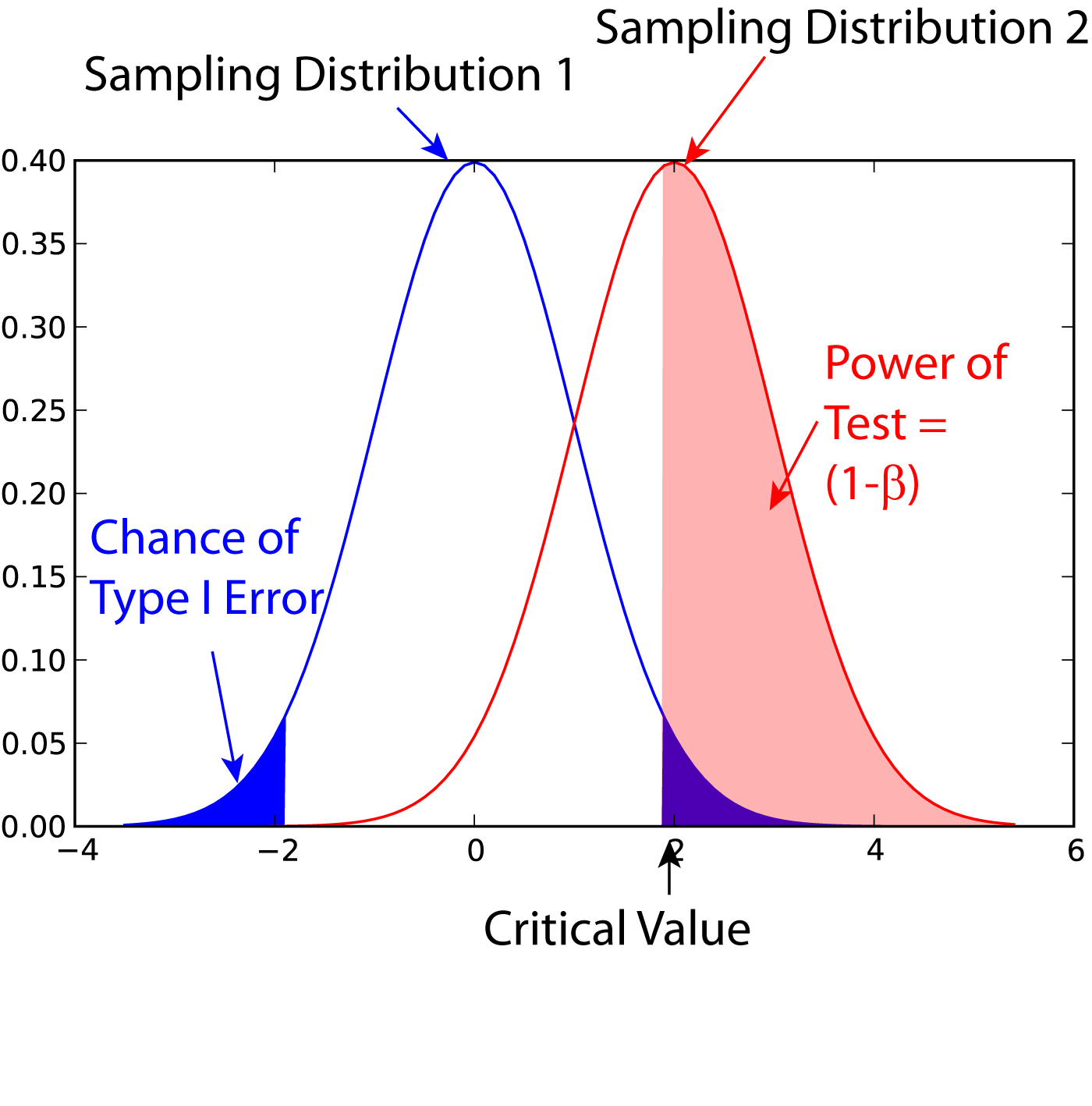
In statistics, the power of a binary hypothesis test is the probability that the test correctly rejects the null hypothesis (H_0) when a specific alternative hypothesis (H_1) is true. It is commonly denoted by 1-\beta, and represents the chances of a true positive detection conditional on the actual existence of an effect to detect. Statistical power ranges from 0 to 1, and as the power of a test increases, the probability \beta of making a type II error by wrongly failing to reject the null hypothesis decreases. Notation This article uses the following notation: * ''β'' = probability of a Type II error, known as a "false negative" * 1 − ''β'' = probability of a "true positive", i.e., correctly rejecting the null hypothesis. "1 − ''β''" is also known as the power of the test. * ''α'' = probability of a Type I error, known as a "false positive" * 1 − ''α'' = probability of a "true negative", i.e., correctly not rejecting the null hypothesis Description For a ty ... [...More Info...] [...Related Items...] OR: [Wikipedia] [Google] [Baidu] |
Type I And Type II Errors
In statistical hypothesis testing, a type I error is the mistaken rejection of an actually true null hypothesis (also known as a "false positive" finding or conclusion; example: "an innocent person is convicted"), while a type II error is the failure to reject a null hypothesis that is actually false (also known as a "false negative" finding or conclusion; example: "a guilty person is not convicted"). Much of statistical theory revolves around the minimization of one or both of these errors, though the complete elimination of either is a statistical impossibility if the outcome is not determined by a known, observable causal process. By selecting a low threshold (cut-off) value and modifying the alpha (α) level, the quality of the hypothesis test can be increased. The knowledge of type I errors and type II errors is widely used in medical science, biometrics and computer science. Intuitively, type I errors can be thought of as errors of ''commission'', i.e. the researcher unluck ... [...More Info...] [...Related Items...] OR: [Wikipedia] [Google] [Baidu] |
Neyman–Pearson Lemma
In statistics, the Neyman–Pearson lemma was introduced by Jerzy Neyman and Egon Pearson in a paper in 1933. The Neyman-Pearson lemma is part of the Neyman-Pearson theory of statistical testing, which introduced concepts like errors of the second kind, power function, and inductive behavior.The Fisher, Neyman-Pearson Theories of Testing Hypotheses: One Theory or Two?: Journal of the American Statistical Association: Vol 88, No 424The Fisher, Neyman-Pearson Theories of Testing Hypotheses: One Theory or Two?: Journal of the American Statistical Association: Vol 88, No 424/ref>Wald: Chapter II: The Neyman-Pearson Theory of Testing a Statistical HypothesisWald: Chapter II: The Neyman-Pearson Theory of Testing a Statistical Hypothesis/ref>The Empire of ChanceThe Empire of Chance/ref> The previous Fisherian theory of significance testing postulated only one hypothesis. By introducing a competing hypothesis, the Neyman-Pearsonian flavor of statistical testing allows investigating the two ... [...More Info...] [...Related Items...] OR: [Wikipedia] [Google] [Baidu] |
Likelihood-ratio Test
In statistics, the likelihood-ratio test assesses the goodness of fit of two competing statistical models based on the ratio of their likelihoods, specifically one found by maximization over the entire parameter space and another found after imposing some constraint. If the constraint (i.e., the null hypothesis) is supported by the observed data, the two likelihoods should not differ by more than sampling error. Thus the likelihood-ratio test tests whether this ratio is significantly different from one, or equivalently whether its natural logarithm is significantly different from zero. The likelihood-ratio test, also known as Wilks test, is the oldest of the three classical approaches to hypothesis testing, together with the Lagrange multiplier test and the Wald test. In fact, the latter two can be conceptualized as approximations to the likelihood-ratio test, and are asymptotically equivalent. In the case of comparing two models each of which has no unknown parameters, use o ... [...More Info...] [...Related Items...] OR: [Wikipedia] [Google] [Baidu] |
Parametrized Family
In mathematics and its applications, a parametric family or a parameterized family is a family of objects (a set of related objects) whose differences depend only on the chosen values for a set of parameters. Common examples are parametrized (families of) functions, probability distributions, curves, shapes, etc. In probability and its applications For example, the probability density function of a random variable may depend on a parameter . In that case, the function may be denoted f_X( \cdot \, ; \theta) to indicate the dependence on the parameter . is not a formal argument of the function as it is considered to be fixed. However, each different value of the parameter gives a different probability density function. Then the ''parametric family'' of densities is the set of functions \ , where denotes the parameter space, the set of all possible values that the parameter can take. As an example, the normal distribution is a family of similarly-shaped distributions par ... [...More Info...] [...Related Items...] OR: [Wikipedia] [Google] [Baidu] |
Probability Density Function
In probability theory, a probability density function (PDF), or density of a continuous random variable, is a function whose value at any given sample (or point) in the sample space (the set of possible values taken by the random variable) can be interpreted as providing a ''relative likelihood'' that the value of the random variable would be close to that sample. Probability density is the probability per unit length, in other words, while the ''absolute likelihood'' for a continuous random variable to take on any particular value is 0 (since there is an infinite set of possible values to begin with), the value of the PDF at two different samples can be used to infer, in any particular draw of the random variable, how much more likely it is that the random variable would be close to one sample compared to the other sample. In a more precise sense, the PDF is used to specify the probability of the random variable falling ''within a particular range of values'', as opposed to ... [...More Info...] [...Related Items...] OR: [Wikipedia] [Google] [Baidu] |
Probability Mass Function
In probability and statistics, a probability mass function is a function that gives the probability that a discrete random variable is exactly equal to some value. Sometimes it is also known as the discrete density function. The probability mass function is often the primary means of defining a discrete probability distribution, and such functions exist for either scalar or multivariate random variables whose domain is discrete. A probability mass function differs from a probability density function (PDF) in that the latter is associated with continuous rather than discrete random variables. A PDF must be integrated over an interval to yield a probability. The value of the random variable having the largest probability mass is called the mode. Formal definition Probability mass function is the probability distribution of a discrete random variable, and provides the possible values and their associated probabilities. It is the function p: \R \to ,1/math> defined by for -\inf ... [...More Info...] [...Related Items...] OR: [Wikipedia] [Google] [Baidu] |
Exponential Family
In probability and statistics, an exponential family is a parametric set of probability distributions of a certain form, specified below. This special form is chosen for mathematical convenience, including the enabling of the user to calculate expectations, covariances using differentiation based on some useful algebraic properties, as well as for generality, as exponential families are in a sense very natural sets of distributions to consider. The term exponential class is sometimes used in place of "exponential family", or the older term Koopman–Darmois family. The terms "distribution" and "family" are often used loosely: specifically, ''an'' exponential family is a ''set'' of distributions, where the specific distribution varies with the parameter; however, a parametric ''family'' of distributions is often referred to as "''a'' distribution" (like "the normal distribution", meaning "the family of normal distributions"), and the set of all exponential families is sometimes l ... [...More Info...] [...Related Items...] OR: [Wikipedia] [Google] [Baidu] |
Sufficiency (statistics)
In statistics, a statistic is ''sufficient'' with respect to a statistical model and its associated unknown parameter if "no other statistic that can be calculated from the same sample provides any additional information as to the value of the parameter". In particular, a statistic is sufficient for a family of probability distributions if the sample from which it is calculated gives no additional information than the statistic, as to which of those probability distributions is the sampling distribution. A related concept is that of linear sufficiency, which is weaker than ''sufficiency'' but can be applied in some cases where there is no sufficient statistic, although it is restricted to linear estimators. The Kolmogorov structure function deals with individual finite data; the related notion there is the algorithmic sufficient statistic. The concept is due to Sir Ronald Fisher in 1920. Stephen Stigler noted in 1973 that the concept of sufficiency had fallen out of favor in descri ... [...More Info...] [...Related Items...] OR: [Wikipedia] [Google] [Baidu] |

