|
RBF Network
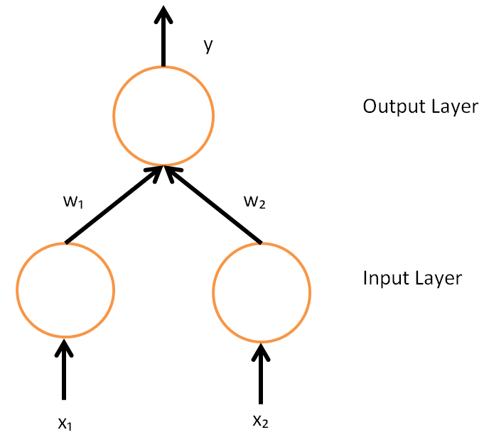
In the field of mathematical modeling, a radial basis function network is an artificial neural network that uses radial basis functions as activation functions. The output of the network is a linear combination of radial basis functions of the inputs and neuron parameters. Radial basis function networks have many uses, including function approximation, time series prediction, classification, and system control. They were first formulated in a 1988 paper by Broomhead and Lowe, both researchers at the Royal Signals and Radar Establishment. Network architecture Radial basis function (RBF) networks typically have three layers: an input layer, a hidden layer with a non-linear RBF activation function and a linear output layer. The input can be modeled as a vector of real numbers \mathbf \in \mathbb^n. The output of the network is then a scalar function of the input vector, \varphi : \mathbb^n \to \mathbb , and is given by :\varphi(\mathbf) = \sum_^N a_i \rho(, , \mathbf-\mathbf_i, , ... [...More Info...] [...Related Items...] OR: [Wikipedia] [Google] [Baidu] |
Mathematical Modeling
A mathematical model is a description of a system using mathematical concepts and language. The process of developing a mathematical model is termed mathematical modeling. Mathematical models are used in the natural sciences (such as physics, biology, earth science, chemistry) and engineering disciplines (such as computer science, electrical engineering), as well as in non-physical systems such as the social sciences (such as economics, psychology, sociology, political science). The use of mathematical models to solve problems in business or military operations is a large part of the field of operations research. Mathematical models are also used in music, linguistics, and philosophy (for example, intensively in analytic philosophy). A model may help to explain a system and to study the effects of different components, and to make predictions about behavior. Elements of a mathematical model Mathematical models can take many forms, including dynamical systems, statistical m ... [...More Info...] [...Related Items...] OR: [Wikipedia] [Google] [Baidu] |
Newton's Method
In numerical analysis, Newton's method, also known as the Newton–Raphson method, named after Isaac Newton and Joseph Raphson, is a root-finding algorithm which produces successively better approximations to the roots (or zeroes) of a real-valued function. The most basic version starts with a single-variable function defined for a real variable , the function's derivative , and an initial guess for a root of . If the function satisfies sufficient assumptions and the initial guess is close, then :x_ = x_0 - \frac is a better approximation of the root than . Geometrically, is the intersection of the -axis and the tangent of the graph of at : that is, the improved guess is the unique root of the linear approximation at the initial point. The process is repeated as :x_ = x_n - \frac until a sufficiently precise value is reached. This algorithm is first in the class of Householder's methods, succeeded by Halley's method. The method can also be extended to complex functions an ... [...More Info...] [...Related Items...] OR: [Wikipedia] [Google] [Baidu] |
Gradient Descent
In mathematics, gradient descent (also often called steepest descent) is a first-order iterative optimization algorithm for finding a local minimum of a differentiable function. The idea is to take repeated steps in the opposite direction of the gradient (or approximate gradient) of the function at the current point, because this is the direction of steepest descent. Conversely, stepping in the direction of the gradient will lead to a local maximum of that function; the procedure is then known as gradient ascent. Gradient descent is generally attributed to Augustin-Louis Cauchy, who first suggested it in 1847. Jacques Hadamard independently proposed a similar method in 1907. Its convergence properties for non-linear optimization problems were first studied by Haskell Curry in 1944, with the method becoming increasingly well-studied and used in the following decades. Description Gradient descent is based on the observation that if the multi-variable function F(\mathbf) is def ... [...More Info...] [...Related Items...] OR: [Wikipedia] [Google] [Baidu] |
Pseudoinverse
In mathematics, and in particular, algebra, a generalized inverse (or, g-inverse) of an element ''x'' is an element ''y'' that has some properties of an inverse element but not necessarily all of them. The purpose of constructing a generalized inverse of a matrix is to obtain a matrix that can serve as an inverse in some sense for a wider class of matrices than invertible matrices. Generalized inverses can be defined in any mathematical structure that involves associative multiplication, that is, in a semigroup. This article describes generalized inverses of a matrix A. A matrix A^\mathrm \in \mathbb^ is a generalized inverse of a matrix A \in \mathbb^ if AA^\mathrmA = A. A generalized inverse exists for an arbitrary matrix, and when a matrix has a regular inverse, this inverse is its unique generalized inverse. Motivation Consider the linear system :Ax = y where A is an n \times m matrix and y \in \mathcal R(A), the column space of A. If A is nonsingular (which implies n ... [...More Info...] [...Related Items...] OR: [Wikipedia] [Google] [Baidu] |
Data Clustering
Cluster analysis or clustering is the task of grouping a set of objects in such a way that objects in the same group (called a cluster) are more similar (in some sense) to each other than to those in other groups (clusters). It is a main task of exploratory data analysis, and a common technique for statistical data analysis, used in many fields, including pattern recognition, image analysis, information retrieval, bioinformatics, data compression, computer graphics and machine learning. Cluster analysis itself is not one specific algorithm, but the general task to be solved. It can be achieved by various algorithms that differ significantly in their understanding of what constitutes a cluster and how to efficiently find them. Popular notions of clusters include groups with small distances between cluster members, dense areas of the data space, intervals or particular statistical distributions. Clustering can therefore be formulated as a multi-objective optimization problem. The ... [...More Info...] [...Related Items...] OR: [Wikipedia] [Google] [Baidu] |
Backpropagation
In machine learning, backpropagation (backprop, BP) is a widely used algorithm for training feedforward neural network, feedforward artificial neural networks. Generalizations of backpropagation exist for other artificial neural networks (ANNs), and for functions generally. These classes of algorithms are all referred to generically as "backpropagation". In Artificial neural network#Learning, fitting a neural network, backpropagation computes the gradient of the loss function with respect to the Glossary of graph theory terms#weight, weights of the network for a single input–output example, and does so Algorithmic efficiency, efficiently, unlike a naive direct computation of the gradient with respect to each weight individually. This efficiency makes it feasible to use gradient methods for training multilayer networks, updating weights to minimize loss; gradient descent, or variants such as stochastic gradient descent, are commonly used. The backpropagation algorithm works by ... [...More Info...] [...Related Items...] OR: [Wikipedia] [Google] [Baidu] |
Regularization (machine Learning)
In mathematics, statistics, finance, computer science, particularly in machine learning and inverse problems, regularization is a process that changes the result answer to be "simpler". It is often used to obtain results for ill-posed problems or to prevent overfitting. Although regularization procedures can be divided in many ways, following delineation is particularly helpful: * Explicit regularization is regularization whenever one explicitly adds a term to the optimization problem. These terms could be priors, penalties, or constraints. Explicit regularization is commonly employed with ill-posed optimization problems. The regularization term, or penalty, imposes a cost on the optimization function to make the optimal solution unique. * Implicit regularization is all other forms of regularization. This includes, for example, early stopping, using a robust loss function, and discarding outliers. Implicit regularization is essentially ubiquitous in modern machine learning appr ... [...More Info...] [...Related Items...] OR: [Wikipedia] [Google] [Baidu] |
Unsupervised Learning
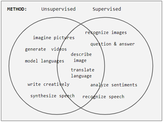
Unsupervised learning is a type of algorithm that learns patterns from untagged data. The hope is that through mimicry, which is an important mode of learning in people, the machine is forced to build a concise representation of its world and then generate imaginative content from it. In contrast to supervised learning where data is tagged by an expert, e.g. tagged as a "ball" or "fish", unsupervised methods exhibit self-organization that captures patterns as probability densities or a combination of neural feature preferences encoded in the machine's weights and activations. The other levels in the supervision spectrum are reinforcement learning where the machine is given only a numerical performance score as guidance, and semi-supervised learning where a small portion of the data is tagged. Neural networks Tasks vs. methods Neural network tasks are often categorized as discriminative (recognition) or generative (imagination). Often but not always, discriminative tas ... [...More Info...] [...Related Items...] OR: [Wikipedia] [Google] [Baidu] |
K-means Clustering
''k''-means clustering is a method of vector quantization, originally from signal processing, that aims to partition ''n'' observations into ''k'' clusters in which each observation belongs to the cluster with the nearest mean (cluster centers or cluster centroid), serving as a prototype of the cluster. This results in a partitioning of the data space into Voronoi cells. ''k''-means clustering minimizes within-cluster variances (squared Euclidean distances), but not regular Euclidean distances, which would be the more difficult Weber problem: the mean optimizes squared errors, whereas only the geometric median minimizes Euclidean distances. For instance, better Euclidean solutions can be found using k-medians and k-medoids. The problem is computationally difficult (NP-hard); however, efficient heuristic algorithms converge quickly to a local optimum. These are usually similar to the expectation-maximization algorithm for mixtures of Gaussian distributions via an iterative refine ... [...More Info...] [...Related Items...] OR: [Wikipedia] [Google] [Baidu] |
Kronecker Delta Function
In mathematics, the Kronecker delta (named after Leopold Kronecker) is a function of two variables, usually just non-negative integers. The function is 1 if the variables are equal, and 0 otherwise: \delta_ = \begin 0 &\text i \neq j, \\ 1 &\text i=j. \end or with use of Iverson brackets: \delta_ = =j, where the Kronecker delta is a piecewise function of variables and . For example, , whereas . The Kronecker delta appears naturally in many areas of mathematics, physics and engineering, as a means of compactly expressing its definition above. In linear algebra, the identity matrix has entries equal to the Kronecker delta: I_ = \delta_ where and take the values , and the inner product of vectors can be written as \mathbf\cdot\mathbf = \sum_^n a_\delta_b_ = \sum_^n a_ b_. Here the Euclidean vectors are defined as -tuples: \mathbf = (a_1, a_2, \dots, a_n) and \mathbf= (b_1, b_2, ..., b_n) and the last step is obtained by using the values of the Kronecker delta ... [...More Info...] [...Related Items...] OR: [Wikipedia] [Google] [Baidu] |
Local Linearity
In mathematics, a differentiable function of one real variable is a function whose derivative exists at each point in its domain. In other words, the graph of a differentiable function has a non-vertical tangent line at each interior point in its domain. A differentiable function is smooth (the function is locally well approximated as a linear function at each interior point) and does not contain any break, angle, or cusp. If is an interior point in the domain of a function , then is said to be ''differentiable at'' if the derivative f'(x_0) exists. In other words, the graph of has a non-vertical tangent line at the point . is said to be differentiable on if it is differentiable at every point of . is said to be ''continuously differentiable'' if its derivative is also a continuous function over the domain of the function f. Generally speaking, is said to be of class if its first k derivatives f^(x), f^(x), \ldots, f^(x) exist and are continuous over the domain of the func ... [...More Info...] [...Related Items...] OR: [Wikipedia] [Google] [Baidu] |


